chapter 4 land cover/ land use mapping using wavelet...

72

CHAPTER 4

LAND COVER/ LAND USE MAPPING USING

WAVELET PACKET TRANSFORM

The images of land received from remote sensing satellites can be

used to derive information on vegetative cover, water bodies, land use pattern,

geological features, soil, etc. Land cover mapping is one of the most

important and typical applications of remote sensing data (image). Land cover

corresponds to the physical condition of the ground surface, for example,

forest, grassland, etc., while land use reflects human activities such as the use

of the land, for example, industrial zones, residential zones, agricultural

fields, etc.

Generally, land cover does not coincide with land use. Land cover

refers to features of land surface, which may be natural, semi-natural,

managed or manmade. They are directly observable by a remote sensor.

A land use class is composed of several land covers, for example, a residential

land use class not only contains built-up class but also contains vegetation

class, water class, etc. The properties measured with remote sensing

techniques relate to land cover, from which land use can be inferred,

particularly with ancillary data or a prior knowledge. Land cover mapping

serves as a basic inventory of land resources for all levels of government,

environmental agencies and private industry throughout the world.

Texture in high resolution satellite images requires substantial

amendment in the conventional segmentation algorithms. This work

73

examined and evaluated the use of wavelet packet transforms for texture

analysis and image classification in high spatial resolution LISS IV imagery.

In this chapter, performance of the combination of WPSFs and WPCFs for the

classification of LISS IV images is discussed. Based on the four indices

(user�s accuracy, producer�s accuracy, overall accuracy and kappa co-

efficient) the accuracy of the classified data is presented.

4.1 PRE PROCESSING

In this work, the advantages of WPT are explored by incorporating

it as a pre-processor for classification. The wavelet packet decomposition is a

generalization of the classical wavelet decomposition and it offers a richer

signal analysis. Here, different wavelet filters such as, Daubechies2 (db2),

Symlet2 (sym2), Coiflet2 (coif2) and Biorthogonal2.2 (bior2.2) wavelet filters

were used for the decomposition of Benchmark (Ahmedabad city) as well as

for the Madurai city. WPT split up the high and low frequencies in equal

bands. The values or transformed co-efficient in detail images are the

essential features useful for texture analysis and discrimination. As micro

textures or macro textures have non-uniform gray level variations, they are

statistically characterized by the features in detail images. In other words, the

features derived from detail images uniquely characterize a texture.

The choice of the H and G filters and its order depends on the

wavelet family used and it varies for different applications. In the proposed

scheme, two levels of wavelet packet decomposition are performed using

different wavelet families as shown in Figure 2.5. The second level of

decomposition provides 16 wavelet coefficient matrices, which represent

quite a huge amount of information (equal to the size of the input image).

It is well known that, as the complexity of a classifier grows rapidly with the

number of dimensions of the pattern space, it is important to take decisions

only on the most essential, so-called discriminatory information, which is

74

conveyed by the extracted features. Each of the 16 coefficient matrices

contains information about the texture of the image.

4.2 PROPOSED SYSTEM

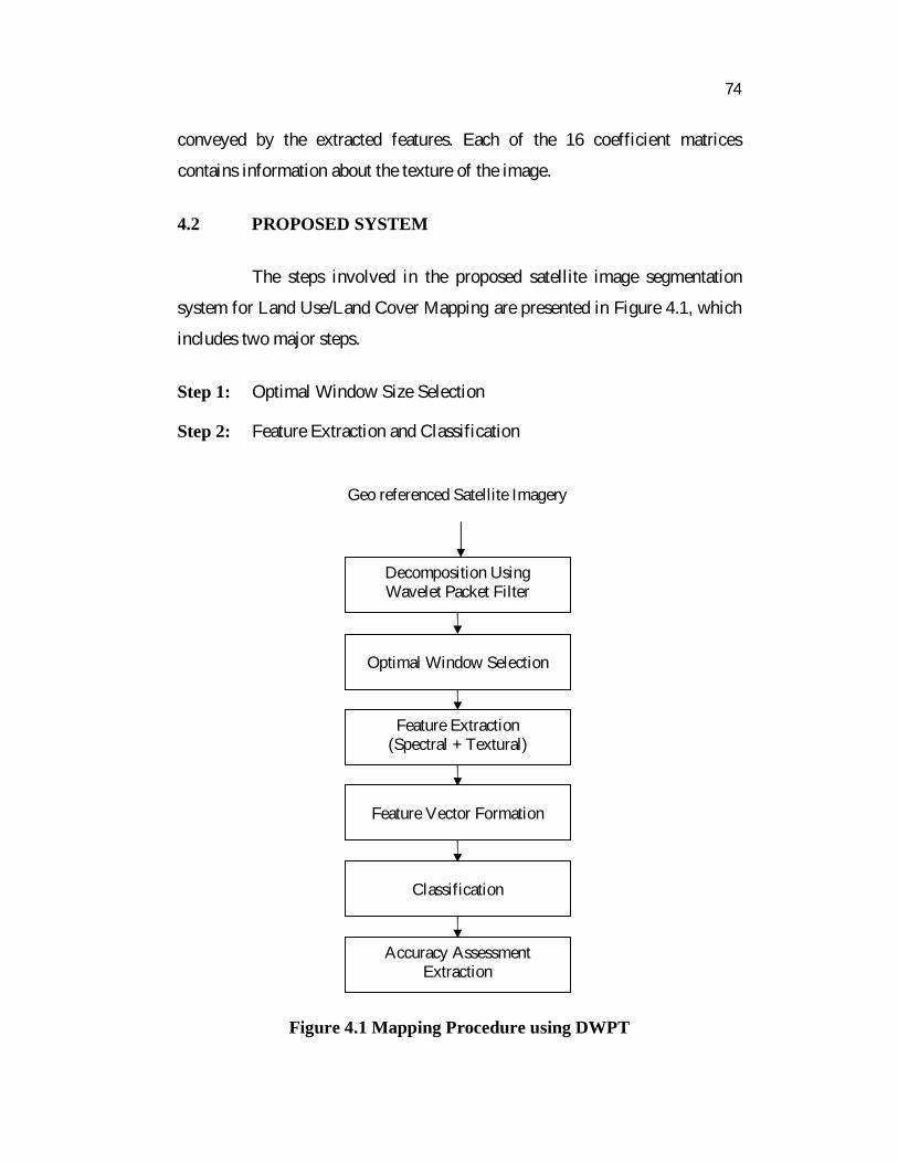
The steps involved in the proposed satellite image segmentation

system for Land Use/Land Cover Mapping are presented in Figure 4.1, which

includes two major steps.

Step 1: Optimal Window Size Selection

Step 2: Feature Extraction and Classification

Figure 4.1 Mapping Procedure using DWPT

Decomposition Using Wavelet Packet Filter

Feature Extraction (Spectral + Textural)

Optimal Window Selection

Accuracy Assessment Extraction

Feature Vector Formation

Classification

Geo referenced Satellite Imagery

75

4.2.1 Optimal Window Size Selection

The success of the classification procedure using textural measures

depends largely on the selected window size (Pesaresi and Benediktsson

2001). Indeed, if the window size is too small, insufficient spatial information

is extracted to characterize a specific land cover and if the window size is too

large, it can overlap two types of ground cover and thus introduce erroneous

spatial information. Therefore, window size for texture analysis is related to

image resolution and the contents within the image. A Geostatistical analysis

indicated that there was no single window size that would adequately

characterize the range of textural conditions that are present in remotely

sensed images (Puissant et al., 2005; Huang et al., 2007). The size of the

processing window is an important issue for spatial feature extraction and

classification of High Resolution satellite imagery. An automatic analysis

system capable of choosing the optimal window size adaptively based on the

multispectral and edge information around the central pixel will greatly

enhance the Classification Accuracy.

Table 4.1 Window Size vs Overall Accuracy

Window Size Overall Accuracy (%)

3 66.78

5 76.96

7 87.6

9 76.00

11 68.90

13 66.00

To facilitate the choice of an optimal texture window, the

coefficient of variation of each texture measure for each thematic class in

76

relation to window size was described (Puissant et al 2005). The chosen

optimal window size is that from which the value of the coefficient of

variation starts to stabilize while having the smallest value (Anys et al 1994).

Therefore, each texture measure identified with its optimal window size is

added in the classification procedure.

Figure 4.2 Window Size vs Overall Accuracy

In this section optimal texture window sizes of different texture

measures are investigated on the test data. By comparing the classification

results for the six window sizes 3 × 3, 5 × 5, 7 × 7, 9 × 9, 11x11 and 13 x13,

as illustrated in Table 4.1 and in Figure 4.2, the highest accuracy is obtained

by the 7 ×7 window. However, it is worth noting that, among the six window

sizes, not all of the information classes reach their highest accuracies with the

7 × 7 window. Larger window with 7 × 7, obtain higher accuracies for

Vegetation and Water Body; however, poor results are obtained for Urban and

Waste land. It seems that the larger window size is reliable for homogeneous

and extensive objects. The 5 × 5 window acquires the highest accuracy for the

Waste land and 3 x 3 windows acquires the highest accuracy for Urban area,

which implies the smaller window size is reliable for heterogeneous regions

or narrow objects. Though a fixed window size is not the most effective for

different information classes, the overall accuracy is higher for the window

77

size 7x7. Moreover, Puissant et al (2005), noted that too small of a window

size results in insufficient information, whereas too large of a window may

overlap multiple features which may introduce erroneous spatial information

and observed that a 7x7 window worked best with high spatial resolution

imagery. Hence, it is chosen as optimal window size for our implementation.

4.2.2 Feature Extraction

Feature extraction is the key for pattern recognition. It is arguably

the most important component in the design of an intelligent system based on

pattern recognition. Even the best classifier will perform poorly if the

features are not chosen well. To select the appropriate features, a number of

experiments were conducted with different features and the results are shown

in the Figures 4.3 to 4.6.

Figure 4.3 Feature vs Producer Figure 4.4 Feature vs Kappa

Figures show that Entropy gives the better results for Overall,

kappa and User accuracy indices and nearer value for Producer accuracy

compared to the others. In order to increase the accuracy further, number of

experiments were conducted with different combinations of features such that

entropy combined with energy, entropy combined with energy and contrast,

78

entropy combined with energy, contrast and correlation, entropy combined

with energy, contrast, correlation and cluster shade, entropy combined with

energy, contrast, correlation, cluster shade and cluster prominence, entropy

combined with energy, contrast, correlation, cluster shade, cluster prominence

and homogeneity.

Experimental results show that the combination of textural features

� entropy (Er), energy (En), contrast (Con), correlation (Cor), cluster shade

(Cs), cluster prominence (Cp) and homogeneity (Hom) greatly improved the

classification results. That is, by using the seven textural features, the

Producer accuracy has increased from around 85.1% to 89.57%, the Kappa

coefficient has increased from 0.78 to 0.82, User accuracy has increased from

82.29% to 82.5% and the overall classification accuracy also has increased

from 84.87% to 87.6 %. The steps involved in texture training and texture

classification are Discrete Wavelet Packet Decomposition (DWPD), wavelet

packet statistical features and wavelet packet co-occurrence features

extraction, spectral feature (NDVI) extraction, feature storage and

classification based on Mahalanobis distance criteria.

Figure 4.5 Feature vs User Figure 4.6 Feature vs Overall

79

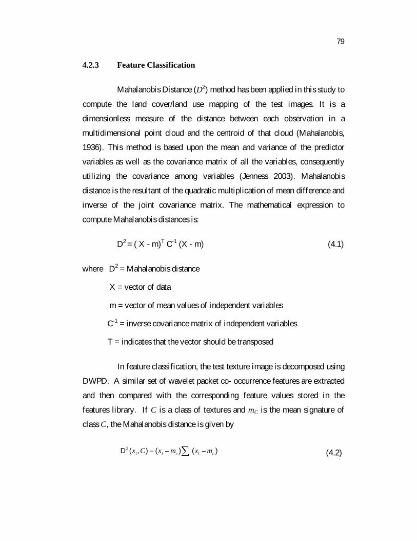
4.2.3 Feature Classification

Mahalanobis Distance (D2) method has been applied in this study to

compute the land cover/land use mapping of the test images. It is a

dimensionless measure of the distance between each observation in a

multidimensional point cloud and the centroid of that cloud (Mahalanobis,

1936). This method is based upon the mean and variance of the predictor

variables as well as the covariance matrix of all the variables, consequently

utilizing the covariance among variables (Jenness 2003). Mahalanobis

distance is the resultant of the quadratic multiplication of mean difference and

inverse of the joint covariance matrix. The mathematical expression to

compute Mahalanobis distances is:

D2 = ( X - m)T C-1 (X - m) (4.1)

where D2 = Mahalanobis distance

X = vector of data

m = vector of mean values of independent variables

C-1 = inverse covariance matrix of independent variables

T = indicates that the vector should be transposed

In feature classification, the test texture image is decomposed using

DWPD. A similar set of wavelet packet co- occurrence features are extracted

and then compared with the corresponding feature values stored in the

features library. If C is a class of textures and mC is the mean signature of

class C, the Mahalanobis distance is given by

)()(),(D2cicii mxmxCx (4.2)

80

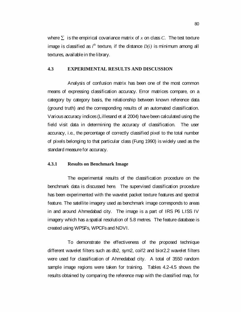
where is the empirical covariance matrix of x on class C. The test texture

image is classified as ith texture, if the distance D(i) is minimum among all

textures, available in the library.

4.3 EXPERIMENTAL RESULTS AND DISCUSSION

Analysis of confusion matrix has been one of the most common

means of expressing classification accuracy. Error matrices compare, on a

category by category basis, the relationship between known reference data

(ground truth) and the corresponding results of an automated classification.

Various accuracy indices (Lillesand et al 2004) have been calculated using the

field visit data in determining the accuracy of classification. The user

accuracy, i.e., the percentage of correctly classified pixel to the total number

of pixels belonging to that particular class (Fung 1990) is widely used as the

standard measure for accuracy.

4.3.1 Results on Benchmark Image

The experimental results of the classification procedure on the

benchmark data is discussed here. The supervised classification procedure

has been experimented with the wavelet packet texture features and spectral

feature. The satellite imagery used as benchmark image corresponds to areas

in and around Ahmedabad city. The image is a part of IRS P6 LISS IV

imagery which has a spatial resolution of 5.8 metres. The feature database is

created using WPSFs, WPCFs and NDVI.

To demonstrate the effectiveness of the proposed technique

different wavelet filters such as db2, sym2, coif2 and bior2.2 wavelet filters

were used for classification of Ahmedabad city. A total of 3550 random

sample image regions were taken for training. Tables 4.2-4.5 shows the

results obtained by comparing the reference map with the classified map, for

81

db2, sym2, coif2 and bior2.2 wavelets and the results are summarized in

Table 4.6. Classified results of the image corresponding to different regions

using db2, sym2, coif 2 and bior2.2 wavelets are illustrated in Figure 4.7.

Table 4.2 Confusion Matrix for Ahmedabad City Image using db2

Cla

ssifi

ed D

ata

Number of

Samples

Reference Data

VegWaterbody

Urban Land

Vegetation 9628 9039 112 477 0

Water body 16563 1361 14952 233 17

Urban 53228 796 2419 48941 1072

Land 7017 53 194 5437 1333

User Accuracy :77.34 Producer Accuracy : 76.91

Overall Accuracy : 83.3 Kappa Coefficient : 0.69

Table 4.3 Confusion Matrix for Ahmedabad City Image using sym2

Cla

ssifi

ed D

ata

Number of

Samples

Reference Data

VegWater body

Urban Land

Vegetation 9628 9322 65 241 0

Water body 16563 1418 13355 1787 3

Urban 53228 1337 5028 46526 337

Land 7017 120 361 6137 399



82

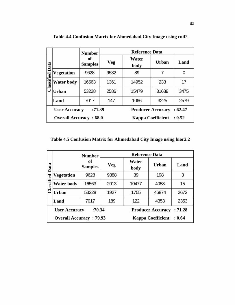
Table 4.4 Confusion Matrix for Ahmedabad City Image using coif2

Cla

ssifi

ed D

ata

Number of

Samples

Reference Data

VegWaterbody

Urban Land

Vegetation 9628 9532 89 7 0

Water body 16563 1361 14952 233 17

Urban 53228 2586 15479 31688 3475

Land 7017 147 1066 3225 2579



Table 4.5 Confusion Matrix for Ahmedabad City Image using bior2.2

Cla

ssifi

ed D

ata

Number of

Samples

Reference Data

VegWater body

Urban Land

Vegetation 9628 9388 39 198 3

Water body 16563 2013 10477 4058 15

Urban 53228 1927 1755 46874 2672

Land 7017 189 122 4353 2353



83

Table 4.6 Results of Different WPT’s for Ahmedabad City

Accuracy Indices

Overall User Producer Kappa

db2 83.3 77.34 76.91 0.69

sym2 80.52 67.63 71.62 0.65

coif2 68.0 71.39 62.47 0.52

bior2.2 79.93 70.34 71.28 0.64

Figure 4.7 Classified Output (a) bior2.2 (b) sym2 (c) db2 (d) coif2

Legend

(a) (b)

(c) (d)

UrbanVegetation Water Body

Land

84

4.3.2 Results on Madurai Image

The above experimental study was carried for LISS IV Madurai

image. A Total of 3550 random sample image regions were taken for training.

For testing, 500 samples were selected randomly from the study area. The

500 samples (pixels) chosen for the experimental study comprises 131, 216,

56, 59, 10 and 4 pixels of urban, vegetation, water body, waste land, tank and

saline land samples, respectively. The 7×7 window size has been used to

extract different wavelet packet co-occurrence based texture features.

The feature set is derived from the original image, all sub bands of

first level of decomposition combined with the features of second level

approximation [A (2, 0)] sub band. The confusion matrices obtained from the

classification results for different wavelet filters are shown in Tables 4.7- 4.11.

Table 4.7 Confusion Matrix for Madurai Image using db2

Cla

ssifi

edD

ata

Numberof

Samples

Reference Data

Urban Veg. Waterbody

Wasteland Tank Saline

LandUrban 131 125 1 1 3 1 0

Vegetation 216 17 189 8 2 0 0

Waterbody 56 0 1 55 0 0 0

WasteLand 59 20 2 1 36 0 0

Tank 10 0 0 0 0 10 0 SalineLand 4 1 1 0 0 0 2

85

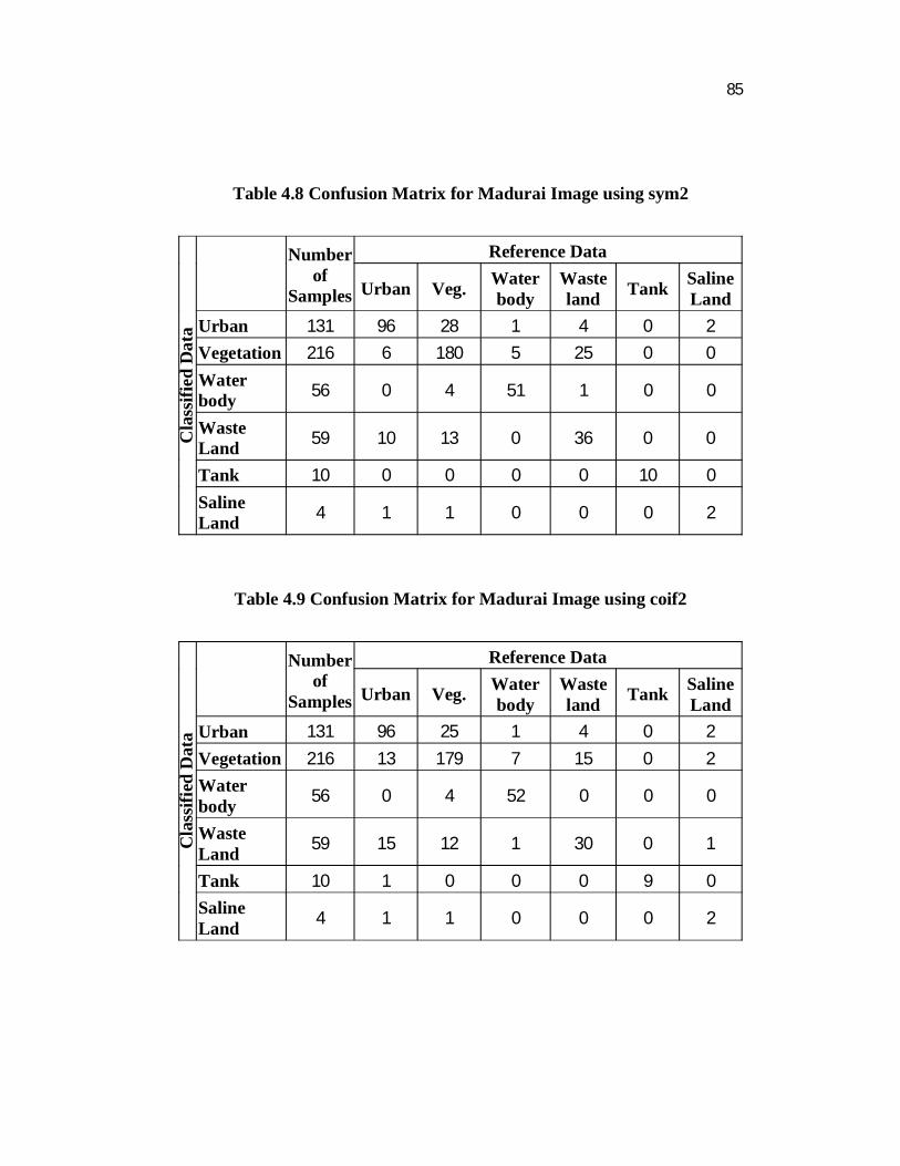
Table 4.8 Confusion Matrix for Madurai Image using sym2 C

lass

ified

Dat

a

Number of

Samples

Reference Data

Urban Veg. Water body


LandUrban 131 96 28 1 4 0 2 Vegetation 216 6 180 5 25 0 0 Waterbody 56 0 4 51 1 0 0

WasteLand 59 10 13 0 36 0 0

Tank 10 0 0 0 0 10 0 SalineLand 4 1 1 0 0 0 2

Table 4.9 Confusion Matrix for Madurai Image using coif2

Cla

ssifi

ed D

ata

Number of

Samples

Reference Data




WasteLand 59 15 12 1 30 0 1

Tank 10 1 0 0 0 9 0 SalineLand 4 1 1 0 0 0 2

86

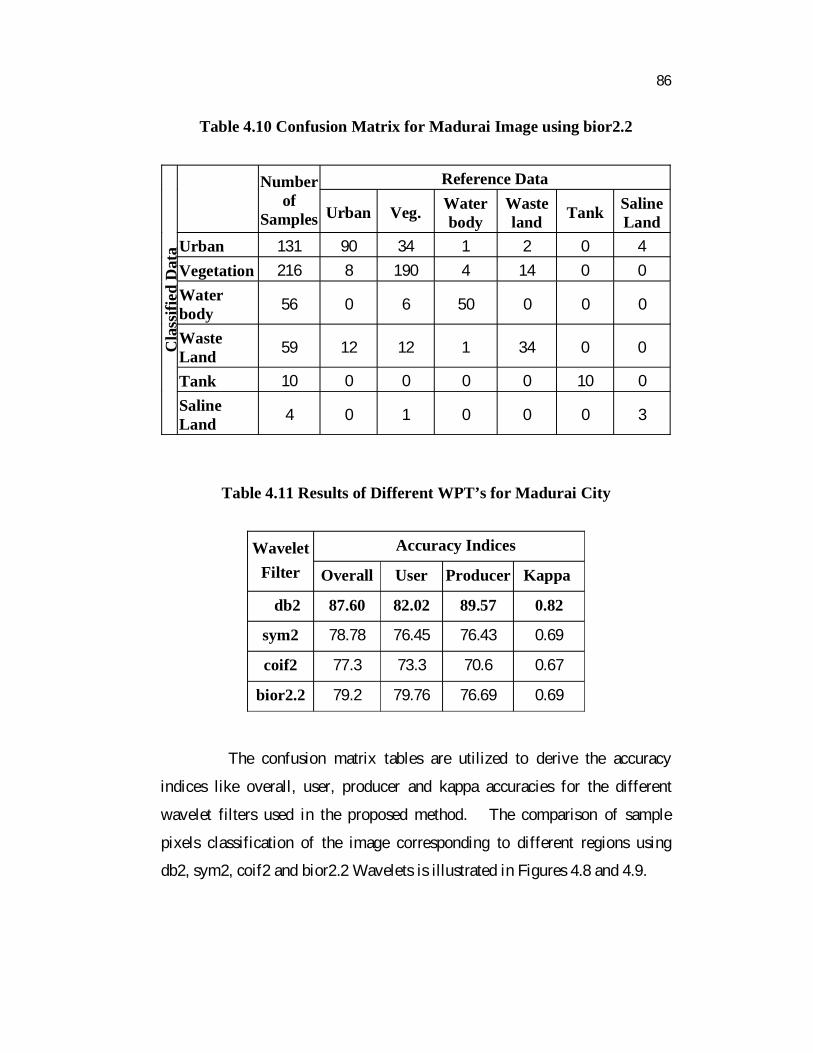
Table 4.10 Confusion Matrix for Madurai Image using bior2.2

Cla

ssifi

ed D

ata

Number of

Samples

Reference Data




WasteLand 59 12 12 1 34 0 0

Tank 10 0 0 0 0 10 0 SalineLand 4 0 1 0 0 0 3

Table 4.11 Results of Different WPT’s for Madurai City

WaveletFilter

Accuracy Indices

Overall User Producer Kappa

db2 87.60 82.02 89.57 0.82

sym2 78.78 76.45 76.43 0.69

coif2 77.3 73.3 70.6 0.67

bior2.2 79.2 79.76 76.69 0.69

The confusion matrix tables are utilized to derive the accuracy

indices like overall, user, producer and kappa accuracies for the different

wavelet filters used in the proposed method. The comparison of sample

pixels classification of the image corresponding to different regions using

db2, sym2, coif2 and bior2.2 Wavelets is illustrated in Figures 4.8 and 4.9.

87

(a) (b)

Figure 4.8 Sample Pixels Classification using Different Wavelet Filters

Figure 4.9 Classified Output using (a) bior2.2 (b) sym2 (c) db2 (d) coif2 (e) db2 without NDVI

88

(c)(d)

(e)

Figure 4.9 (Continued)

4.4 SUMMARY

Daubechies2, Symlet2, Coiflet2 and Biorthogonal2.2 wavelets were

used in this study for land cover/ land use mapping using high resolution

LISS IV imagery. Daubechies wavelets are compactly supported wavelets

with extremal phase and highest number of vanishing moments for a given

support width. Associated scaling filters are minimum-phase filters. Symlets

wavelets are compactly supported wavelets with least asymmetry and highest

89

number of vanishing moments for a given support width. Associated scaling

filters are near linear-phase filters. Coiflets wavelets are compactly supported

wavelets with highest number of vanishing moments for both phi and psi for a

given support width. Biorthogonal wavelets are compactly supported

biorthogonal spline wavelets for which symmetry and exact reconstruction are

possible with FIR filters (in orthogonal case it is impossible except for Haar).

Experiments were done using the benchmark (Ahmedabad City)

and Madurai images for optimal window selection. From the experimental

results, as shown in Table 4.1, a window size of 7 x 7 is observed to be the

better option to measure the different wavelet packet co-occurrence based

texture features. The results obtained provide a higher classification rate of

87.6% which is obtained for the feature set comprising wavelet packet

statistical features, mean and standard deviation and a set of wavelet packet

co-occurrence features contrast, energy, entropy, local homogeneity, cluster

shade, cluster prominence and correlation derived from the original, first level

of decomposition combined with the features of second level approximation

[A(2,0)] sub band. In this work, the samples were selected randomly from the

homogenous texture regions. Also this work confirms the utility of both

textural and spectral analysis to enhance the per-pixel classification accuracy

for high resolution images, especially in urban areas where the images are

spectrally more heterogeneous. Though, different wavelets perform better for

different applications, from the empirical analysis of the experimental results

obtained for the benchmark (Ahmedabad) and Madurai images, it is observed

that Daubechies2 capture features of satellite imagery in a better manner

compared to other wavelets.

chapter 4 land cover/ land use mapping using wavelet...

Documents