JOINT REGRESSION MODELING OF TWO

CUMULATIVE INCIDENCE FUNCTIONS UNDER

AN ADDITIVITY CONSTRAINT

AND

STATISTICAL ANALYSES OF PILL-MONITORING

DATA

by

Martin P. Houze

B. Sc. University of Lyon, 2000

M. A. Applied Statistics, University of Pittsburgh, 2009

Submitted to the Graduate Faculty of

the Kenneth P. Dietrich School Of Arts and Sciences in partial

fulfillment

of the requirements for the degree of

Doctor of Philosophy

University of Pittsburgh

2015

UNIVERSITY OF PITTSBURGH

THE KENNETH P. DIETRICH SCHOOL OF ARTS AND SCIENCES

This dissertation was presented

by

Martin P. Houze

It was defended on

Apr 16th, 2015

and approved by

Yu Cheng, Associate Professor, Department of Statistics and Department of Psychiatry

Satish Iyengar, Professor, Department of Statistics

Leon J. Gleser, Professor, Department of Statistics

Jong-Hyeon Jeong, Professor, Department of Biostatistics

Dissertation Advisors: Yu Cheng, Associate Professor, Department of Statistics and

Department of Psychiatry,

Satish Iyengar, Professor, Department of Statistics

ii

Copyright c© by Martin P. Houze

2015

iii

JOINT REGRESSION MODELING OF TWO CUMULATIVE INCIDENCE

FUNCTIONS UNDER AN ADDITIVITY CONSTRAINT

AND

STATISTICAL ANALYSES OF PILL-MONITORING DATA

Martin P. Houze, PhD

University of Pittsburgh, 2015

In the first part of this dissertation, we propose a parametric regression model for cumu-

lative incidence functions (CIFs) which are commonly used for competing risks data. Our

parametric model adopts several parametric functions as baseline CIFs and a proportional

hazard or a generalized odds rate model for covariate effects. This parametric model ex-

plicitly takes into account the additivity constraint that a subject should eventually fail

from one of the causes so the asymptotes of the CIFs should add up to one. Our primary

goal is to propose a parametric regression model that provides regression parameters for the

CIFs of both the primary and secondary risks. Moreover, we introduce a modified Weibull

baseline distribution. The inference procedure is straightforward. Parameters are estimated

via the maximization of the likelihood. Standard errors are obtained via the Hessian of the

log-likelihood. We demonstrate the good practical performance of this parametric model.

We simulate the underlying processes for cause 1 and cause 2, and compare our models with

some existing methods.

In the second part of this dissertation, we propose several approaches for the modeling and

analysis of medication bottle opening events data, and focus on frailty models, in both

parametric and semiparametric forms. This approach provides regression coefficients which

iv

are of great interest to investigators and clinicians. A time effect can also be estimated. We

apply our approaches to the analysis of a medication bottle opening events data set. To our

knowledge, this is the first study of prescription bottle opening events which focuses on time

between medication administrations through frailty models. We discuss the interpretation

of the random effect of a subject, and how it can help characterize the adherence of that

individual relative to that of the other subjects. We then present an exploratory cluster

analysis of the survival curves of the participants.

v

TABLE OF CONTENTS

1.0 JOINT REGRESSION MODELING OF TWO CUMULATIVE INCI-

DENCE FUNCTIONS UNDER AN ADDITIVITY CONSTRAINT . 1

1.1 Introduction . . . . . . . . . . . . . . . . . . . . . . . . . . . . . . . . . . . 1

1.2 Model formulation . . . . . . . . . . . . . . . . . . . . . . . . . . . . . . . . 3

1.2.1 Modified logistic baseline with PH link function . . . . . . . . . . . . 5

1.2.2 Modified Weibull baseline with PH link function . . . . . . . . . . . . 6

1.2.3 Modified logistic baseline with GOR link function . . . . . . . . . . . 7

1.2.4 Modified Weibull baseline with GOR link function . . . . . . . . . . . 9

1.3 Simulations . . . . . . . . . . . . . . . . . . . . . . . . . . . . . . . . . . . . 10

1.4 Breast Cancer study data analysis . . . . . . . . . . . . . . . . . . . . . . . 15

1.4.1 Cause 1 regression coefficients . . . . . . . . . . . . . . . . . . . . . . 16

1.4.2 Cause 2 regression coefficients . . . . . . . . . . . . . . . . . . . . . . 17

1.4.3 Model Discussion . . . . . . . . . . . . . . . . . . . . . . . . . . . . . 24

2.0 STATISTICAL ANALYSES OF PILL-MONITORING DATA . . . . . 25

2.1 Introduction . . . . . . . . . . . . . . . . . . . . . . . . . . . . . . . . . . . 25

2.2 Models . . . . . . . . . . . . . . . . . . . . . . . . . . . . . . . . . . . . . . 28

2.2.1 Modeling of gap times . . . . . . . . . . . . . . . . . . . . . . . . . . . 28

2.2.1.1 Cox regression . . . . . . . . . . . . . . . . . . . . . . . . . . . 29

2.2.1.2 Accelerated failure time models . . . . . . . . . . . . . . . . . 29

2.2.1.3 Frailty models with nonparametric baseline function . . . . . . 29

2.2.1.4 Modeling of the random effects . . . . . . . . . . . . . . . . . 31

vi

2.2.1.5 Cox frailty model with time-varying covariate . . . . . . . . . 32

2.2.1.6 Frailty models with parametric baseline function . . . . . . . . 32

2.2.2 Counting processes . . . . . . . . . . . . . . . . . . . . . . . . . . . . 33

2.2.2.1 Bayesian estimation of Cox regression with random effects . . 33

2.2.3 Software . . . . . . . . . . . . . . . . . . . . . . . . . . . . . . . . . . 34

2.3 Analysis of data . . . . . . . . . . . . . . . . . . . . . . . . . . . . . . . . . 35

2.3.1 Exploratory data analysis . . . . . . . . . . . . . . . . . . . . . . . . . 36

2.3.2 Proportional hazard assumption . . . . . . . . . . . . . . . . . . . . . 40

2.3.3 Model comparison and covariate selection . . . . . . . . . . . . . . . . 40

2.3.4 Interpretation of the random effect . . . . . . . . . . . . . . . . . . . . 41

2.3.5 Model validation . . . . . . . . . . . . . . . . . . . . . . . . . . . . . . 46

2.4 Exploratory cluster analysis . . . . . . . . . . . . . . . . . . . . . . . . . . . 47

2.4.1 Spline regression . . . . . . . . . . . . . . . . . . . . . . . . . . . . . . 47

2.4.1.1 Cubic splines . . . . . . . . . . . . . . . . . . . . . . . . . . . 47

2.4.1.2 Natural smoothing splines . . . . . . . . . . . . . . . . . . . . 48

2.4.2 Application to the ACT/CARE study dataset . . . . . . . . . . . . . 48

2.4.2.1 Clustering using ID-level summary measure . . . . . . . . . . 48

2.4.2.2 Functional data clustering . . . . . . . . . . . . . . . . . . . . 49

2.5 Conclusion and future work . . . . . . . . . . . . . . . . . . . . . . . . . . . 50

3.0 BIBLIOGRAPHY . . . . . . . . . . . . . . . . . . . . . . . . . . . . . . . . . 52

vii

LIST OF TABLES

1.1 Simulation results where the data were simulated from our proposed modified

logistic (panel LOG + PH) or Weibull model (panel WEI + PH) with comple-

mentary log-log transformation or with generalized odds-rate transformation

(panel LOG + GOR and WEI + GOR), where AVE is the average of the

estimates, MoSE is the average of the model-based standard errors, ESE is

the empirical standard error, and Cov is the coverage rates of the 95% Wald

CIs . . . . . . . . . . . . . . . . . . . . . . . . . . . . . . . . . . . . . . . . . 13

1.2 The estimates of the Causes 1 and 2 regression coefficients for the Breast

Cancer Study based on our proposed modified logistic (Log) and the modified

Weibull (Wei) with generalized odds-rate transformation, and the Fine-Gray

model (FG). . . . . . . . . . . . . . . . . . . . . . . . . . . . . . . . . . . . . 18

1.3 The estimates of the Cause 2 regression coefficients for the Breast Cancer

Study based on the Fine-Gray model (FG), the Fine-Gray model with tumor

size by time interaction (FGt), and the stratified Fine-Gray model (SFG) . . 22

2.1 Parametric models . . . . . . . . . . . . . . . . . . . . . . . . . . . . . . . . . 44

2.2 Frailty models with non parametric baseline hazard . . . . . . . . . . . . . . 45

2.3 Descriptive statistics of clusters . . . . . . . . . . . . . . . . . . . . . . . . . 50

viii

LIST OF FIGURES

1.1 Estimates of CIFs for two example patients using the breast cancer study dataset 19

1.2 Estimates of time-varying coefficient for age in the cause 2 regression using

the Breast cancer study dataset . . . . . . . . . . . . . . . . . . . . . . . . . 20

1.3 Estimates of time-varying coefficient for treatment in the cause 2 regression

using the Breast cancer study dataset . . . . . . . . . . . . . . . . . . . . . . 21

1.4 Estimates of time-varying coefficient for tumor size in the cause 2 regression

using the Breast cancer study dataset . . . . . . . . . . . . . . . . . . . . . . 21

1.5 Nonparametric estimates of cause 2 CIF curves for Placebo and Tamoxifen

groups . . . . . . . . . . . . . . . . . . . . . . . . . . . . . . . . . . . . . . . 23

2.1 Histogram of gap times . . . . . . . . . . . . . . . . . . . . . . . . . . . . . . 37

2.2 Histogram of log gap times. . . . . . . . . . . . . . . . . . . . . . . . . . . . 37

2.3 ID 1328's individual survival curve. . . . . . . . . . . . . . . . . . . . . . . . 38

2.4 ID 1517's individual survival curve. . . . . . . . . . . . . . . . . . . . . . . . 39

2.5 Survival curve for the entire sample . . . . . . . . . . . . . . . . . . . . . . . 40

2.6 Survival curves by gender. . . . . . . . . . . . . . . . . . . . . . . . . . . . . 41

2.7 ID 1139's individual survival curve. . . . . . . . . . . . . . . . . . . . . . . . 42

2.8 Profile likelihood for the individual random effect model . . . . . . . . . . . . 43

2.9 Survival curves of first and last gap times . . . . . . . . . . . . . . . . . . . . 46

2.10 Clusters . . . . . . . . . . . . . . . . . . . . . . . . . . . . . . . . . . . . . . 49

2.11 Individual survival curve with spline . . . . . . . . . . . . . . . . . . . . . . . 50

ix

Acknowledgments

I want to thank my advisors, Pr. Yu Cheng and Pr. Satish Iyengar, for their guidance.

I express my gratitude to Pr. Leon Gleser for his support during my years as a graduate

student. I also thank the members of my committee for the time they invested in reading

my manuscript, and in providing me with important feedback.

Finally I want to thank Pr. Susan Sereika and Pr. Jacqueline Dunbar-Jacob for their

encouragement and for giving me access to the dataset of the Evaluation of Adherence

Interventions in Clinical Trials study.

x

1.0 JOINT REGRESSION MODELING OF TWO CUMULATIVE

INCIDENCE FUNCTIONS UNDER AN ADDITIVITY CONSTRAINT

1.1 INTRODUCTION

Cox regression models (Cox, 1972b) and accelerated failure time models (Wei et al., 1990; Jin

et al., 2003) are commonly used to analyze covariate effects on a single variable measuring

the time to an event. In many survival studies, there are several competing causes of failure.

The primary event, or the event of interest, may not be observed if the other competing

events occur first. For example, in the breast cancer study considered by Shi et al. (2013),

the primary event is the recurrence of a cancer growing locally. But this primary event may

be unobservable, or competing-risk censored, if the other events such as death or distant

metastasis have occurred first. In many other studies, investigators are interested in analyz-

ing the time to death due to a certain disease of interest. However some of the participants

will die from causes other than the disease of interest, for instance other diseases or trauma.

Hence it is of interest to take the cause of death into account and carry out cause-specific

analyses.

In a competing risks setting, some standard quantities such as the survival function may

not be well defined if removal of competing events is not conceptually realistic (Gooley et al.,

1999). Instead, the cumulative incidence function (CIF) has been an established quantity

to describe cumulative risks of an event of interest over time (Kalbfleisch and Prentice,

2002). The limit of a CIF is less than one, and is thus often referred to as subdistribu-

tion. Another approach in competing risks studies with covariates involves modeling the

cause-specific hazard functions via a proportional hazards assumption (Prentice et al., 1978;

1

Beyersmann et al., 2012). Unfortunately, the cause-specific hazard function does not have a

direct interpretation in terms of survival probabilities for the particular failure type (Pepe,

1991; Gaynor et al., 1993). Many clinicians prefer using the CIF because it is intuitively

appealing and more easily understood by the nonstatistician.

Shi et al. (2013) point out that all subdistributions, or CIFs, should add up to one when

time goes to infinity, as one subject should eventually die from one of the competing causes.

Shi et al. (2013) also note that such additivity constraint is ignored in some commonly used

regression models for CIFs, such as the semi-parametric models of Fine and Gray (1999)

and Scheike et al. (2008), which only consider one event at a time. If several causes are of

interest, one may run their models several times (one iteration for each cause). However, it is

not clear how to interpret the sets of regression parameters when the CIFs do not add up to

one as time goes to infinity (Shi et al., 2013). Jeong and Fine (2007) presented a parametric

model based on CIFs, but did not seem to account for the constraint either.

We consider two causes K = 1, 2, one for the event of interest, and the other for the

competing event. Let T and C be the event time and censoring time. Let t denote time, and

z the covariates. Shi et al. (2013) presented a parametric model for simultaneous inference

of two CIFs. Their model adopts a modified logistic model as the baseline CIF and a

generalized odds-rate model for covariate effects. Moreover, it explicitly takes into account

the additivity constraint that a subject should eventually fail from one of the causes, so that

the asymptotes of the CIFs should add up to one,

P (K = 1|z) + P (K = 2|z) = 1. (1.1.1)

However Shi et al. (2013) did not explicitly model the covariate effects on the competing

cause. Rather, they specified the covariate effects on the competing cause indirectly through

the covariate effects on the primary cause and the additivity constraint.

Our primary goal is to propose a parametric regression model that is based on the frame-

work of Jeong and Fine (2007) and Shi et al. (2013), but provides regression parameters for

the CIFs of both the primary and secondary risks. Our model also accounts for the afore-

mentioned additivity constraint (1.1.1). Moreover, we update the model of Shi et al. (2013)

2

by introducing a new baseline function: the modified Weibull CIF. The Weibull distribution

has been widely used in industrial and biomedical applications (Klein and Moeschberger,

2003), and is especially useful in modeling time to appearance of tumors in humans (Doll,

1971). However it cannot be directly used to model time to local cancer recurrence in our

breast cancer application, because of competing-risk censoring. We hence introduce an extra

leveling-off parameter in the modified Weibull CIF. The modified Weibull CIF can take a

range of shapes with one or two bendpoints. Some Weibull CIF curves are of concave in-

creasing shape, other curves are of sigmoidal shape, similar to the modified logistic function

(Cheng, 2009).

The rest of the document is organized as follows. We introduce our parametric models

in Section 1.2. Extensive simulation studies are performed in Section 1.3 to compare the

performance of our parametric model with the Fine and Gray (1999) method, the semipara-

metric model by Scheike et al. (2008) and the parametric model in Jeong and Fine (2007).

We applied all these regression models to the datasets of a breast cancer study in section

1.4.

1.2 MODEL FORMULATION

Let C be the censoring time, T be the time to an event, and K = 1, 2 be the cause indicator.

We observe Y = min(T,C) and η = KI{T < C}, where I is the indicator function. Let Zk

be a covariate vector with respect to the cause k event, k = 1, 2. Fine and Gray (1999) and

Fine (2001) assume that

gk{Fk(t; βk, Z)} = gk{F0k(t)}+ βkZ, (1.2.1)

where gk is some nondecreasing known function, and F0k(t) = Fk(t;Z = 0) is an invertible

and monotonically increasing function. The commonly used Fine and Gray method considers

g(u) = log{− log(1− u)}, (1.2.2)

3

which gives a proportional hazards interpretation for subdistribution hazards.

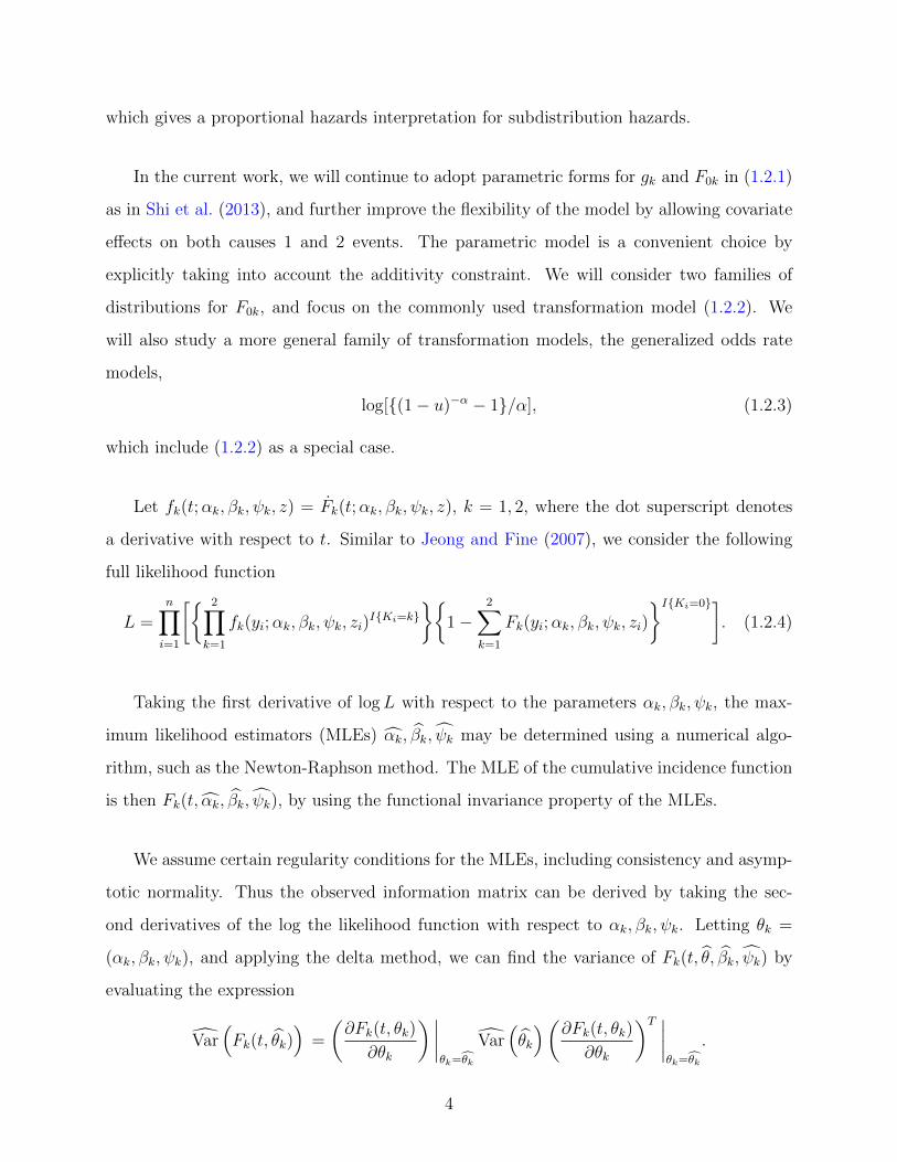
In the current work, we will continue to adopt parametric forms for gk and F0k in (1.2.1)

as in Shi et al. (2013), and further improve the flexibility of the model by allowing covariate

effects on both causes 1 and 2 events. The parametric model is a convenient choice by

explicitly taking into account the additivity constraint. We will consider two families of

distributions for F0k, and focus on the commonly used transformation model (1.2.2). We

will also study a more general family of transformation models, the generalized odds rate

models,

log[{(1− u)−α − 1}/α], (1.2.3)

which include (1.2.2) as a special case.

Let fk(t;αk, βk, ψk, z) = Fk(t;αk, βk, ψk, z), k = 1, 2, where the dot superscript denotes

a derivative with respect to t. Similar to Jeong and Fine (2007), we consider the following

full likelihood function

L =n∏i=1

[{ 2∏k=1

fk(yi;αk, βk, ψk, zi)I{Ki=k}

}{1−

2∑k=1

Fk(yi;αk, βk, ψk, zi)

}I{Ki=0}]. (1.2.4)

Taking the first derivative of logL with respect to the parameters αk, βk, ψk, the max-

imum likelihood estimators (MLEs) αk, βk, ψk may be determined using a numerical algo-

rithm, such as the Newton-Raphson method. The MLE of the cumulative incidence function

is then Fk(t, αk, βk, ψk), by using the functional invariance property of the MLEs.

We assume certain regularity conditions for the MLEs, including consistency and asymp-

totic normality. Thus the observed information matrix can be derived by taking the sec-

ond derivatives of the log the likelihood function with respect to αk, βk, ψk. Letting θk =

(αk, βk, ψk), and applying the delta method, we can find the variance of Fk(t, θ, βk, ψk) by

evaluating the expression

Var(Fk(t, θk)

)=

(∂Fk(t, θk)

∂θk

) ∣∣∣∣θk=θk

Var(θk

)(∂Fk(t, θk)∂θk

)T ∣∣∣∣θk=θk

.

4

Because θk = (αk, βk, ψk),∂Fk(t,θk)∂θk

is equivalent to(∂Fk(t, θk)

∂αk,∂Fk(t, θk)

∂βk,∂Fk(t, θk)

∂ψk

).

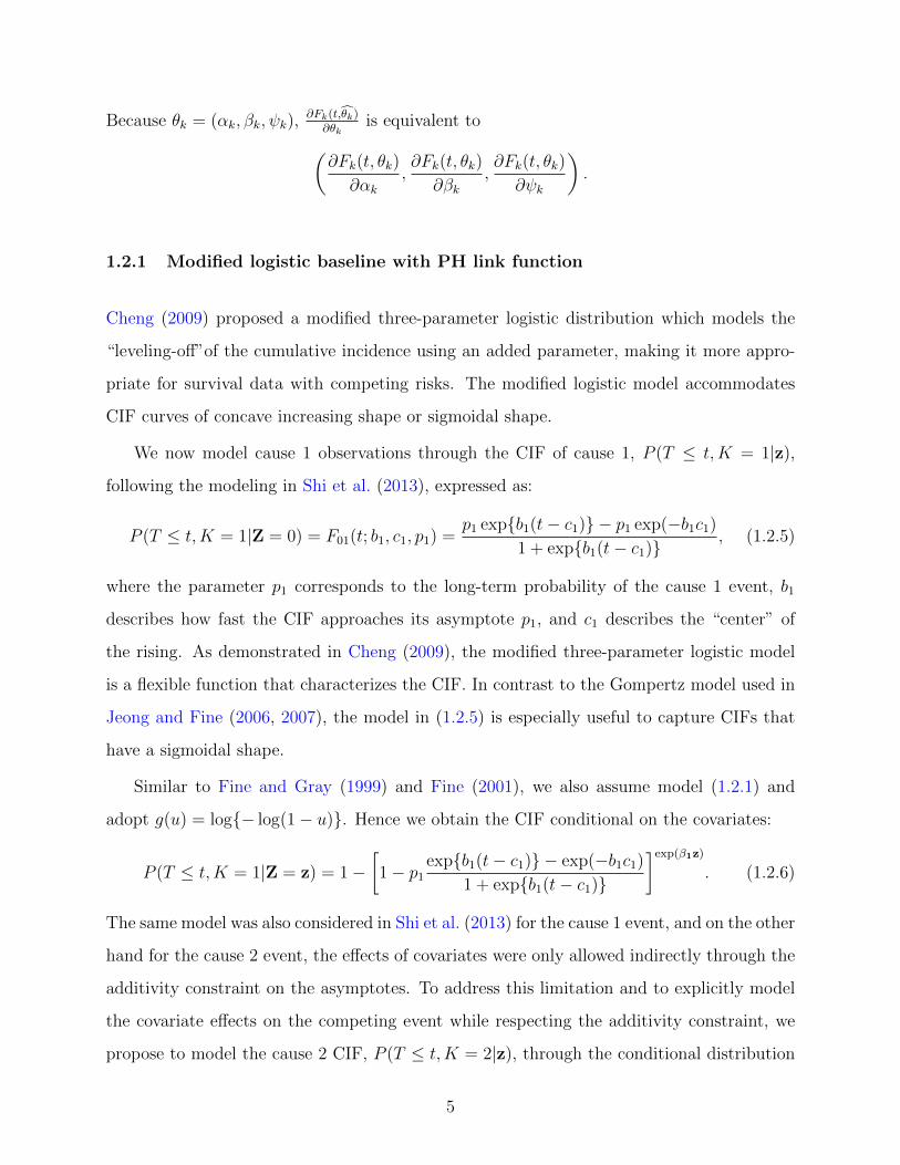
1.2.1 Modified logistic baseline with PH link function

Cheng (2009) proposed a modified three-parameter logistic distribution which models the

“leveling-off”of the cumulative incidence using an added parameter, making it more appro-

priate for survival data with competing risks. The modified logistic model accommodates

CIF curves of concave increasing shape or sigmoidal shape.

We now model cause 1 observations through the CIF of cause 1, P (T ≤ t,K = 1|z),

following the modeling in Shi et al. (2013), expressed as:

P (T ≤ t,K = 1|Z = 0) = F01(t; b1, c1, p1) =p1 exp{b1(t− c1)} − p1 exp(−b1c1)

1 + exp{b1(t− c1)}, (1.2.5)

where the parameter p1 corresponds to the long-term probability of the cause 1 event, b1

describes how fast the CIF approaches its asymptote p1, and c1 describes the “center” of

the rising. As demonstrated in Cheng (2009), the modified three-parameter logistic model

is a flexible function that characterizes the CIF. In contrast to the Gompertz model used in

Jeong and Fine (2006, 2007), the model in (1.2.5) is especially useful to capture CIFs that

have a sigmoidal shape.

Similar to Fine and Gray (1999) and Fine (2001), we also assume model (1.2.1) and

adopt g(u) = log{− log(1− u)}. Hence we obtain the CIF conditional on the covariates:

P (T ≤ t,K = 1|Z = z) = 1−[1− p1

exp{b1(t− c1)} − exp(−b1c1)

1 + exp{b1(t− c1)}

]exp(β1z)

. (1.2.6)

The same model was also considered in Shi et al. (2013) for the cause 1 event, and on the other

hand for the cause 2 event, the effects of covariates were only allowed indirectly through the

additivity constraint on the asymptotes. To address this limitation and to explicitly model

the covariate effects on the competing event while respecting the additivity constraint, we

propose to model the cause 2 CIF, P (T ≤ t,K = 2|z), through the conditional distribution

5

P (T ≤ t|K = 2, z). That is,

P (T ≤ t,K = 2|z) = P (T ≤ t|K = 2, z)×P (K = 2|z) = P (T ≤ t|K = 2, z)×p2(z), (1.2.7)

where p2(z) is set by the constraint P (K = 1|z) + P (K = 2|z) = 1.

Note that P (T ≤ t|K = 2, z) is a proper conditional distribution which approaches 1 as

time goes to∞. Hence, we can use any of the existing parametric regression models for sur-

vival data, such as linear models for log time or the transformation models similar to (1.2.1)

except now the distributions are proper. Meanwhile, the modified logistic function can be

easily adapted to accommodate proper distribution functions by dropping the “leveling-off”

parameter, yielding the modified logistic function for the baseline conditional distribution:

P (T ≤ t|K = 2,Z = 0) = CDF02(t) =exp{b2(t− c2)} − exp(−b2c2)

1 + exp{b2(t− c2)}. (1.2.8)

If we again choose the log-log link function g(u) = log{− log(1− u)}, we have

P (T ≤ t|K = 2, z) = CDF2(t) = 1−[1− exp{b2(t− c2)} − exp(−b2c2)

1 + exp{b2(t− c2)}

]exp(β2z)

. (1.2.9)

We now use (1.2.7) and the additivity constraint in order to find p2(z). Due to the

additivity constraint for the baseline CIFs, F01(∞) + F02(∞) = 1, p2(z = 0) = 1 − p1. For

any given covariates z, again by the additivity constraint F1(∞, z) + F2(∞, z) = 1, we have

1− (1− p1)exp(β1z) + (1− (0)exp(β2z))× p2(z) = 1− (1− p1)exp(β1z) + p2(z) = 1,

and thus p2(z) = (1 − p1)exp(β1z). Coupled with the conditional model in (1.2.9), we can

explicitly model the covariate effects on the cause 2 CIF F2(t) as

P (T ≤ t,K = 2|z) = (1− p1)exp(β1z) ×{

1−[1− exp{b2(t− c2)} − exp(−b2c2)

1 + exp{b2(t− c2)}

]exp(β2z)}.

1.2.2 Modified Weibull baseline with PH link function

As we have discussed in the introduction, we also consider a modified Weibull distribution for

baseline CIFs, in addition to the modified logistic function. The Weibull distribution is used

extensively in applications to model survival times (Klein and Moeschberger, 2003), since

6

the Weibull curves can have one, or two bend points. We modify the Weibull distribution

to describe the baseline cause 1 CIF:

F01(t; k1, λ1, p1) = P (T ≤ t,K = 1|Z = 0) = p1{1− e−(t/λ1)k1}, (1.2.10)

where k1 > 0 is the shape parameter, λ1 > 0 is the scale parameter of the distribution, and

p1 controls the asymptote of the CIF.

Using the modified Weibull baseline CIF and the log-log link function in (1.2.1), we

obtain the CIF conditional on the covariates:

P (T ≤ t,K = 1|Z = z) = 1− (1− p1[1− exp{−(t/λ1)k1}])exp(β1.z).

We then turn to the modeling of cause 2 data following the strategy in (1.2.7). We start

by defining the cause 2 conditional distribution at baseline as

P (T ≤ t|K = 2,Z = 0) = CDF02(t) = 1− e−(t/λ2)k2 . (1.2.11)

If we again choose the log-log link function g(u) = log{− log(1− u)}, we obtain

P (T ≤ t|K = 2, z) = 1− {e−(t/λ2)k2}exp(β2.z).

Similarly to the previous model, the additivity constraint F01(∞) + F02(∞) = 1 results in

p2(z) = (1− p1)exp(β1.z). Therefore, the cause 2 conditional CIF F2(t) is given below:

P (T ≤ t,K = 2|z) = (1− p1)exp(β1.z) × {1− [e−(t/λ2)k2 ]exp(β2.z)}.

1.2.3 Modified logistic baseline with GOR link function

The above two modeling strategies were derived based on the log-log link function which is

equivalent to the proportional subdistribution hazard assumption for the cause 1 CIF, and

the proportional hazard assumption for the conditional distribution given the competing

event being the cause of failure. These assumptions may not be realistic in some applications.

Hence we consider a more general transformation function in (1.2.3), which includes the log-

log link as a special case.

7

We begin the modeling of cause 1 observations with the same baseline modified logistic

CIF F01(t) as in (1.2.5). The generalized odds rate link has inverse function g−11 (u) =

1− {α1 exp(u) + 1}−1/α1 . Then we have

P (T ≤ t,K = 1|z) = g−11 [g1{F01(t)}+ β1z].

We now turn to the modeling of the secondary risk quantities. Similarly as before, we

consider the baseline conditional distribution in (1.2.8).

We want to bring covariate effects into our modeling. We use link function g2(u) =

log[{(1 − u)−α2 − 1}/α2], which has inverse function g−12 (u) = 1 − (α2 × exp(u) + 1)−1/α2 ,

and obtain:

P (T ≤ t|K = 2, z) = CDF2(t) = g−12 [g2(CDF02) + β2z].

We now write out F1(∞):

F01(∞) = 1− {α1 × exp(log[{(1− p1)−α1 − 1}/α1] + β1z) + 1}−1/α1 .

Shifting to cause 2 CIF, we have F2(∞, z) = p2(z)× P (T ≤ ∞|K = 2, z) = p2(z).

Therefore the covariate-adjusted additivity constraint F1(∞, z)+p2(z)×CDF2(∞, z) = 1

results in p2(z) = 1− F1(∞, z).

Hence we have the following expression for p2(z) = {α1 × exp(log[{(1 − p1)−α1 − 1}/α1] +

β1z) + 1}−1/α1 .

Using the expression of p2(z) obtained from the covariate-adjusted additivity constraint,

we can write out the cause 2 CIF F2(t) as

P (T ≤ t,K = 2|z) ={α1 × exp(log[{(1− p1)−α1 − 1}/α1] + β1z) + 1}−1/α1

× g−12 (g2(CDF02) + β2z)).

That is, we explicitly model the covariate effects on the competing cause.

8

1.2.4 Modified Weibull baseline with GOR link function

We begin the modeling of cause 1 observations with the same baseline CIF as in (1.2.10),

and for cause 2 data we use the baseline Weibull CDF as in (1.2.11).

We now need to incorporate covariate effects in the modeling of the secondary risk data.

To do so, we use link function g2(u) = log[{(1− u)−α2 − 1}/α2], which has inverse function

g−12 (u) = 1− (α2 × exp(u) + 1)−1/α2 , and obtain:

P (T ≤ t|K = 2, z) = g−12 [g2(CDF02) + β2z],

where CDF02 = P (T ≤ t|K = 2,Z = 0) = {1− e−(t/λ2)k2}.

We now compute F1(∞).

F1(∞) = 1− {α1 ∗ exp(log[{(1− p1)−α1 − 1}/α1] + β1z) + 1}−1/α1 .

Shifting to cause 2 CIF, and using the same additivity constraint as in the previous

model, we obtain p2(z) = {α1 × exp(log[{(1− p1)−α1 − 1}/α1] + β1z) + 1}−1/α1 .

Using p2 = 1−p1 which we obtained from the baseline CIF additivity constraint, we can

write out the baseline cause 2 CIF, denoted F02, as follows

P (T ≤ t,K = 2|z = 0) = (1− p1)(1− e−(t/λ2)k2 ).

Using the expression of p2(z) obtained from the covariate-adjusted additivity constraint,

we can write out the cause 2 CIF F2(t) and explicitly model the covariate effects on the

competing cause:

P (T ≤ t,K = 2|z) ={α1 × exp(log[{(1− p1)−α1 − 1}/α1] + β1z) + 1}−1/α1

× g−12 (g2[1− e−(t/λ2)k2 ] + β2z)).

Some datasets may require a flexible model. The baseline CIF functions for cause 1 and

cause 2 do not have to be from the same parametric family. For instance, the modified

Weibull baseline function can be chosen for cause 1 events, while the modified logistic can be

chosen for cause 2 events. Furthermore, the regression can utilize the proportional hazards

approach for cause 1 data, and the generalized odds rate approach for cause 2 data.

9

1.3 SIMULATIONS

We perform extensive simulation studies to evaluate the finite-sample performance of our

parametric regression models using the modified logistic function (LOG), and the modified

Weibull function (WEI) as compared to the Fine and Gray method (FG) and the time-

varying coefficients model proposed by Scheike et al. (Sch). Several scenarios are considered.

We let the baseline CIFs satisfy either a modified logistic function (LOG), or a Weibull

(WEI) function. The covariate effects follow a proportional hazard model for hazards of

sub-distribution (PH). Below we give details on how we simulate the data with the LOG

baseline and PH effects (LOG+PH). We assume that the baseline CIF for the primary cause

follows (1.2.5) with k = 1. The regression model on the cause 1 CIF satisfies g{F1(t; z)} =

g{F01(t)} + β1z, where z1 and z2 are drawn from the standard normal distribution and

g(u) = log{− log(1 − u)}. Then the cause 1 CIF conditional on the covariates z′

= (z1, z2)

has the form of (1.2.6) and β′1 = (β11, β12). Therefore, we simulate the event time by

F−11 (U ; z), where U ∼ uniform(0, 1) and F−1

1 is the inverse function of F1(t; z). Note that

F1 is improper and may not be invertible. When U < 1 − (1 − p1)exp(β′1z), we simulate the

event time by

T = F−11 (U ; z) = c1 +

1

b1

log

{1− (1− U)exp(−β′

1z) + p1 exp{−b1c1}p1 − 1 + (1− U)exp(−β′

1z)

},

with K = 1. When U ≥ 1 − (1 − p1)exp(β′1z), K = 2 and the event time T comes from the

cause 2 event.

As mentioned in Section 1.2, one needs to keep the additivity constraint (1.1.1). Thus,

for the competing cause (K = 2), the conditional distribution of T given K = 2 is

F (t|K = 2, z) = P (T ≤ t|K = 2, z) = 1−[1− exp{b2 × (t− c2)} − exp(−b2 × c2)

1 + exp{b2 × (t− c2)}]exp(β2.z)

.

Then we simulate the event time T by F−1(V |K = 2, z), where F−1 is the inverse func-

tion of F and V ∼uniform(0,1). We also simulate independent censoring time C follow-

ing uniform(a, b), where a and b are constants greater than zero. The observable time is

Y = min(T,C) and the corresponding cause indicator is η = KI{T < C}. Different values

10

of a and b are used and the percentage of censoring is around 15-25% for all our simulations.

In each run of our simulations, we generate 300 pairs of event times and associated cause

indicators. Next, we fit the simulated data by using our proposed parametric model with

the modified logistic (LOG) baseline and the PH transformation, and the modified Weibull

(WEI) and the PH transformation.

For the parametric models, the regression coefficient estimates are obtained by using the

R function “nlminb” to minimize the minus likelihood function (1.2.4). nlminb() performs

optimization subject to box constraints (i.e. upper and/or lower constraints on individual

elements of the parameter vector). The variance of the estimator is estimated via the inverse

of the Information matrix. The Information matrix is the negative of the expected value of

the Hessian matrix, the matrix of second derivatives of the likelihood with respect to the

parameters. The inverse is calculated via the R function “solve.” For the semi-parametric

models, we use the R function “crr” in the package cmprsk (Fine and Gray, 1999) and the

R function “comp.risk” in the package timereg (Scheike et al., 2008; Scheike and Zhang,

2011).

We first show simulations using our modified logistic regression model. The results from

2, 500 simulations are summarized in table 1.1. In each table, we report the averages of the

estimates (AVE), the model-based standard errors (MoSE) which are computed based on the

observed Fisher information matrices, the empirical standard errors (ESE), and the coverage

(Cov) rates of the 95% asymptotic Wald confidence intervals for the regression coefficients

and the CIFs evaluated at times 3 and 5, given that the covariates are Z1 = −1 and Z2 = 2.

The Scheike et al. (2008) model does not provide regression coefficients for covariates

like the LOG, WEI or Fine Gray models. Instead, the Scheike method provides time-varying

coefficients. As a consequence, we did not use the Scheike model when comparing regression

coefficients and their standard errors across different models.

Table 1.1 contains the results for the cause 1 and cause 2 regression coefficients β11, β12,

β21, and β22 from the two parametric models and the Fine and Gray model, as well as the

cause 1 and cause 2 CIFs F1(1), F1(3), F2(1), and F2(3) from the two parametric models,

the Fine and Gray model and the Scheike model. The true model is marked in bold letters

11

in the leftmost column of the table.

When handling the LOG+PH data, as presented in panels A1 and A2 of table 1.1, our

modified logistic model has comparable or better performance than Fine and Gray’s semi-

parametric model, when it comes to estimating regression coefficients and predicting CIFs.

The Fine and Gray model shows downward bias when estimating the cause 2 regression

coefficients. To evaluate the effect of misspecifying baseline CIFs when estimating regression

coefficients and predicting CIFs, we generate the data based on a modified logistic base-

line and the proportional hazard model (LOG+PH). We then apply our proposed modified

Weibull regression model to the simulated LOG+PH data and report estimation statistics in

table 1.1. The estimation converges without significant bias, and the MoSEs are reasonable,

which is evidence that the Weibull estimation procedure has some robustness. However,

when we apply the modified Weibull baseline model to the simulated modified logistic data,

the optimization takes more time (approximately twice longer) to converge, when compared

to estimating with the modified logistic model.

We also run simulations using our modified Weibull regression model. The results from

2, 500 simulations are summarized in panels B1 and B2 of table 1.1. When the baseline CIFs

are from the modified Weibull model, the performance of our proposed modifed logistic model

is comparable to that of the modified Weibull model and of the Fine and Gray method. The

more general method by Scheike et al. (2008) also performs well, although the standard errors

provided by the package are noticeably larger than the ones from the other three models.

As shown in table 1.1, the semiparametric model of Fine and Gray (1999) underestimates

the values of β21 and β22, the regression coefficients of cause 2. As a result, the coverage of

the Wald confidence intervals is very low.

Next, we evaluate and compare the performance of the models when the proportional

hazards assumption does not hold. We adopt the generalized odds rate (GOR) transforma-

tion (Dabrowska and Doksum, 1998; Jeong and Fine, 2007) for cause 1 and cause 2 CIFs.

That is, g{F1(t; z);α1} = g{F01(t);α1}+β′1z, where g{ν;α1} = log[{(1−ν)−α1−1}/α1]. We

set α1 = 5 in our simulations. We simulate the competing cause times using α2 = 5. We con-

12

Table 1.1: Simulation results where the data were simulated from our proposed modified logistic(panel LOG + PH) or Weibull model (panel WEI + PH) with complementary log-log transformationor with generalized odds-rate transformation (panel LOG + GOR and WEI + GOR), where AVEis the average of the estimates, MoSE is the average of the model-based standard errors, ESE isthe empirical standard error, and Cov is the coverage rates of the 95% Wald CIs

LOG + PH β11 β12 F1(1) F1(3)

DIM VAR Log Wei FG Log Wei FG Log Wei FG Sch Log Wei FG Sch

300

(A1) True 0.50 0.50 0.50 0.50 0.50 0.50 0.08 0.08 0.08 0.08 0.15 0.15 0.15 0.15

AVE 0.50 0.51 0.50 0.50 0.50 0.50 0.08 0.09 0.09 0.09 0.15 0.15 0.14 0.14MoSE 0.11 0.11 0.11 0.11 0.11 0.11 0.02 0.03 0.09 0.33 0.04 0.04 0.06 0.37ESE 0.11 0.11 0.11 0.11 0.11 0.11 0.02 0.03 0.08 0.08 0.04 0.04 0.05 0.05Cov 0.95 0.94 0.95 0.94 0.95 0.94 0.93 0.92 0.98 0.98 0.94 0.95 1.00 1.00

WEI + PH β11 β12 F1(1) F1(3)

300

(B1) True 0.50 0.50 0.50 0.50 0.50 0.50 0.19 0.19 0.19 0.19 0.35 0.35 0.35 0.35

AVE 0.51 0.51 0.50 0.49 0.51 0.50 0.18 0.19 0.19 0.19 0.35 0.36 0.36 0.36MoSE 0.11 0.11 0.11 0.11 0.11 0.11 0.04 0.04 0.09 0.32 0.07 0.08 0.10 0.18ESE 0.10 0.11 0.11 0.12 0.11 0.11 0.04 0.04 0.07 0.07 0.07 0.07 0.08 0.08Cov 0.96 0.95 0.95 0.88 0.94 0.94 0.90 0.94 0.90 1.00 0.91 0.94 0.90 0.99

LOG + GOR β11 β12 F1(1) F1(3)

300

(C1) True 0.50 0.50 0.50 0.50 0.50 0.50 0.08 0.08 0.08 0.08 0.14 0.14 0.14 0.14

AVE 0.50 0.52 0.24 0.51 0.52 0.24 0.08 0.08 0.09 0.09 0.15 0.16 0.14 0.14MoSE 0.24 0.26 0.11 0.25 0.26 0.11 0.03 0.03 0.06 0.36 0.13 0.14 0.07 0.36ESE 0.21 0.21 0.11 0.21 0.21 0.11 0.03 0.03 0.06 0.08 0.04 0.05 0.07 0.06Cov 0.93 0.94 0.32 0.94 0.94 0.31 0.91 0.92 0.92 0.99 0.96 0.97 0.92 1.00

WEI + GOR β11 β12 F1(1) F1(3)

300

(D1) True 0.50 0.50 0.50 0.50 0.50 0.50 0.16 0.16 0.16 0.16 0.29 0.29 0.29 0.29

AVE 0.50 0.53 0.26 0.48 0.53 0.26 0.16 0.16 0.16 0.16 0.29 0.29 0.29 0.29MoSE 0.24 0.25 0.11 0.25 0.25 0.11 0.05 0.05 0.06 0.34 0.19 0.19 0.06 0.20ESE 0.19 0.23 0.11 0.19 0.24 0.11 0.04 0.05 0.06 0.06 0.04 0.05 0.07 0.07Cov 0.94 0.91 0.42 0.96 0.91 0.41 0.90 0.89 0.92 1.00 0.96 0.95 0.92 1.00

LOG + PH β21 β22 F2(1) F2(3)

DIM VAR Log Wei FG Log Wei FG Log Wei FG Sch Log Wei FG Sch

300

(A2) True 0.50 0.50 0.50 0.50 0.50 0.50 0.32 0.32 0.32 0.32 0.48 0.48 0.48 0.48

AVE 0.51 0.48 -0.04 0.51 0.49 -0.04 0.32 0.32 0.32 0.32 0.47 0.47 0.43 0.43MoSE 0.09 0.09 0.08 0.09 0.09 0.08 0.07 0.06 0.20 0.20 0.07 0.07 0.07 0.13ESE 0.10 0.09 0.08 0.10 0.09 0.08 0.07 0.06 0.08 0.08 0.07 0.07 0.07 0.07Cov 0.94 0.96 0.00 0.95 0.95 0.00 0.94 0.94 1.00 1.00 0.94 0.94 1.00 1.00

WEI + PH β21 β22 F2(1) F2(3)

300

(B2) True 0.50 0.50 0.50 0.50 0.50 0.50 0.31 0.31 0.31 0.31 0.51 0.51 0.51 0.51

AVE 0.51 0.52 -0.03 0.51 0.51 -0.03 0.31 0.31 0.28 0.28 0.51 0.50 0.47 0.47MoSE 0.10 0.09 0.08 0.10 0.10 0.08 0.06 0.06 0.09 0.21 0.07 0.09 0.10 0.11ESE 0.10 0.10 0.08 0.11 0.10 0.08 0.06 0.06 0.07 0.07 0.07 0.08 0.07 0.07Cov 0.95 0.95 0.00 0.95 0.95 0.00 0.96 0.94 0.90 1.00 0.95 0.94 0.90 0.99

LOG + GOR β21 β22 F2(1) F2(3)

300

(C2) True 0.50 0.50 0.50 0.50 0.50 0.50 0.26 0.26 0.26 0.26 0.46 0.46 0.46 0.46

AVE 0.51 0.58 -0.10 0.51 0.58 -0.09 0.27 0.27 0.26 0.26 0.46 0.47 0.47 0.47MoSE 0.28 0.32 0.07 0.29 0.32 0.07 0.06 0.06 0.07 0.23 0.13 0.14 0.07 0.11ESE 0.24 0.27 0.07 0.23 0.27 0.07 0.06 0.06 0.07 0.07 0.05 0.05 0.07 0.07Cov 0.95 0.96 0.00 0.96 0.96 0.00 0.94 0.94 0.92 1.00 0.96 0.97 0.95 0.98

WEI + GOR β21 β22 F2(1) F2(3)

300

(D2) True 0.50 0.50 0.50 0.50 0.50 0.50 0.29 0.29 0.29 0.29 0.51 0.51 0.51 0.51

AVE 0.45 0.52 -0.07 0.51 0.52 -0.07 0.29 0.29 0.29 0.29 0.52 0.51 0.51 0.51MoSE 0.28 0.29 0.07 0.29 0.29 0.07 0.06 0.06 0.07 0.21 0.18 0.19 0.07 0.10ESE 0.27 0.26 0.07 0.19 0.26 0.07 0.06 0.06 0.07 0.07 0.05 0.05 0.07 0.07Cov 0.94 0.92 0.00 0.98 0.92 0.00 0.92 0.90 0.92 1.00 0.97 0.95 0.95 0.97

13

sider both the modified logistic and modified Weibull functions for the baseline CIFs when

generating the data. We then fit our modified logistic and modified Weibull models with the

generalized odds-rate transformation, the Fine and Gray method and the semiparametric

model by Scheike et al. (2008) to the simulated LOG+GOR and WEI+GOR data.

When estimating the LOG+GOR data, our modified logistic model does well, although

the Fine Gray model has lower MoSEs when estimating F1(3) and F2(3), as seen in panels

C1 and C2 of table 1.1. We estimate a relatively high number of parameters (the center of

rising and steepness of the two baseline models, the four regression coefficients, α1 and α2).

This allows us to test our parametric model in conditions similar to those of the analysis of

a new dataset. The somewhat higher MoSEs of some of the predictions obtained from the

parametric models may be a reflection the number of parameters in the model. As before,

the Scheike model tends to overestimate the standard errors in their CIF estimators. The

modified Weibull model can handle data generated from the modified logistic baseline model,

although the MoSEs when estimating the regression coefficients are a bit higher than when

using the modified logistic model.

As the proportional hazards assumption is clearly violated, the Fine and Gray method

results in downward bias when estimating covariate effects. Because the Fine and Gray

model is a semiparametric approach, the misspecified covariate effects may be compensated

by the nonparametric estimation of the baseline CIF. As a consequence, the predicted CIF

is close to the true value despite the misspecified covariate effects.

We now turn to the WEI+GOR simulations presented in panels D1 and D2 of table

1.1. Again, our modified Weibull model does quite well, although the MoSEs for F1(3) and

F2(3) are larger than those of the Fine and Gray model. The modified logistic model again

does well when used to estimate data generated from the Weibull baseline model. The Fine

and Gray method again seriously underestimates regression coefficients, although its CIFs

predictions are satisfactory. When the true data are from the modified Weibull model, the

modified logistic model performs well. Our modified Weibull model performs just as well

as the modified logistic model does. Both work well for the sample of size 300 and clearly

outperform the general semiparametric model by Scheike et al. (2008). The Scheike model

14

overestimates the variability in predicting CIFs, so that its coverage rate is close to 1. The

coverage rates of regression parameters from the Fine and Gray method are much lower than

the nominal level.

1.4 BREAST CANCER STUDY DATA ANALYSIS

Having developed our modeling framework, we now turn to applying our proposed models to

the National Surgical Adjuvant Breast and Bowel Project Breast Cancer Study (NSABP B-

14). This study investigated the effects of tamoxifen for node negative and hormonal receptor

positive patients. The data contain information on time (in years), event (0=censored,

1=recurrence, 2=other events), treatment group (trt=1, placebo; trt=2, tamoxifen), age,

and tumor size (through variable tsize), for 2,582 eligible patients who had follow-up and

known tumor sizes. Recurrence is the event of interest and other events are treated as

competing ones.

Of the 2,582 patients enrolled in the study, 1,276 (49.4 %) were censored, 577 (22.3 %)

had a recurrence of their cancer, and 729 (28.2 %) had other events. 1299 (50.3 %) of the

study participants were in the placebo group, whereas 1283 (49.7 %) of the participants were

in the tamoxifen group. The age of the participants ranges between 25 and 75 years of age

with a median of 56 years of age and an interquartile range (IQR) of 16 years. Tumor size

ranges between 3 and 135, with a median of 20 and an IQR of 13. Tumor size shows 18 mild

outliers. These observations are identified as mild outliers because they are greater than

75th% tile +1.5× IQR. Tumor size also shows 9 severe outliers, defined as such because they

are greater than 75th% tile +3 × IQR. Hence, tumor size is top-coded before running the

analyses. That is, the top 10% of tumor size values are set respectively to the value of the

1st 90th percentile. Topcoding is often called censoring. Censoring and robustness methods

are presented in Tukey (1979b) and Tukey (1979a).

We investigate the statistical associations among covariates. The placebo and tamoxifen

groups are well-balanced when considering the age of the participants. A t-test fails to reject

15

the hypothesis of equal average age across the treatment groups (t=.34, p=.73). The median

age is 57 years (IQR=16 years) in the placebo group, and 54.8 years (IQR=15 years) in the

treatment group. A t-test fails to reject the hypothesis of equal average tumor size across the

treatment groups (t=-.43, p=.67). Median tumor size is 20 (IQR=14) in the placebo group,

and 20 (IQR=12). Tumor size has more severe outliers (8) in the tamoxifen group than in

the placebo group (1). The mild outliers of tumor size are more or less evenly distributed

among the two randomization groups. The correlation between age and tumor size is small

(-.05), but statistically significant (p=.01).

Before fitting the data, we code trt=0 for placebo and trt=1 for tamoxifen, and center

the age at mean 55 and tumor size at mean 22. The likelihood is maximized on all the

parameters of the two distribution, as well as on α1 and α2. We fit cause 1 and cause 2

regressions simultaneously, but for clarity’s sake, we present the results separately in the

following sections. We emphasize the presentation of the competing cause because Shi et al.

(2013) investigated cause 1 in details.

1.4.1 Cause 1 regression coefficients

The cause 1 coefficients in our work are modeled in a fashion similar to that of Shi et al.

(2013). As expected, the cause 1 coefficients we estimated were very close to those of Shi

et al. (2013).

We first run the Kolmogorov-Smirnov test and the Cramer von Mises test for time in-

variant effects of treatment group, age and tumor size (Scheike et al., 2008). The assumption

of proportional hazards for subdistribution does not hold for age. Hence we apply our mod-

ified logistic model and the modified Weibull model with the GOR transformation to the

breast cancer data. The Fine and Gray (1999) model is also included for comparison because

our simulations suggest that this model can have good prediction on CIFs even though the

estimates of the regression coefficients may be biased.

As shown in table 1.2, the cause 1 coefficient estimates and standard errors obtained

from the modified logistic model and the modified Weibull model are generally close to each

other, and the coefficient estimates from the Fine and Gray model are a bit larger than those

16

from the parametric models. However, the p values from the three models are comparable

and fairly small for all three prognostic factors. The coefficients for treatment and age are

all negative while those for tumor size are all positive across the three models. This suggests

that the patients who were older, received Tamoxifen treatment and had smaller tumor sizes

were less likely to have cancer recurrence.

Next, we select two patient cases to compare the predicted CIFs from the four models.

Patient I has good prognostic factors: Tamoxifen (trt = 1), 65 years old (age = 10) and

tumor size 12 (tsize = -10), while patient II has poor prognostic factors: placebo (trt = 0),

45 years old (age = -10) and tumor size 32 (tsize = 10). The four predicted CIFs are plotted

in Figure 1.1. The solid lines are the estimated CIFs from 0 to 20 years from the modified

logistic model, the dashed lines are for the modified Weibull model and the dotted lines are

from Fine and Gray’s model. The estimated CIFs of the Scheike semiparametric model are

represented by the gray lines. We first observe that the CIF curves only have one bend point.

The predicted 20 years recurrence rate is somewhere between 0.1 and 0.2 for patient I and

somewhere between 0.3 and 0.4 for patient II based on the parametric and the Fine Gray

models. In the figure, we also include the confidence bands (gray dashed lines) from the

Scheike et al. model, which are available from the R package timereg. The estimated CIFs

of the parametric models and of the Fine Gray models lie between the confidence bands of

the Scheike et al. model, though the confidence bands are likely to be conservative.

An exploratory Cox regression is run to evaluate the covariate effects on the hazard of

local recurrence. The coefficients in the Cox regression were consistent with those of the

CIF-based analyses.

1.4.2 Cause 2 regression coefficients

We first run the Kolmogorov-Smirnov test and the Cramer von Mises test for time invariant

effects of treatment group, age and tumor size (Scheike et al., 2008).

The assumption of proportional hazards for subdistribution holds for age. On the left-

hand panel of figure 1.2, we show the time-varying coefficient estimate for age (solid line)

along with its 95 % pointwise confidence intervals (broken lines) and 95% confidence bands

17

Table 1.2: The estimates of the Causes 1 and 2 regression coefficients for the Breast Cancer Studybased on our proposed modified logistic (Log) and the modified Weibull (Wei) with generalizedodds-rate transformation, and the Fine-Gray model (FG).

β1 trt β1 age β1 tsize

VAR Log Wei FG Log Wei FG Log Wei FG

Est -0.82 -0.69 -0.48 -0.02 -0.02 -0.01 0.04 0.05 0.02

Stderr 0.16 0.15 0.09 0.01 0.007 0.004 0.01 0.010 0.003

Z -5.15 -4.68 -5.60 -3.22 -3.38 -2.58 6.05 4.94 7.40

p value <0.001 <0.001 <0.001 <0.001 <0.001 0.01 <0.001 <0.001 <0.001

β2 trt β2 age β2 tsize

VAR Log Wei FG Log Wei FG Log Wei FG

Est -0.23 -0.63 0.02 0.038 0.021 0.03 0.013 0.013 -0.005

Stderr 0.15 0.17 0.07 0.007 0.006 0.004 0.007 0.006 0.003

Z -1.50 -3.66 0.23 5.86 3.31 7.50 1.95 1.74 -1.67

p value 0.13 <0.001 0.81 <0.001 <0.001 <0.001 0.06 0.08 0.10

18

5 10 15 20

0.0

0.1

0.2

0.3

0.4

0.5

0.6

Time

Pro

babi

lity

Patient I. Local Recurrence

Mod Logistic

Mod Weibull

Fine−Gray

Scheike

5 10 15 20

0.0

0.1

0.2

0.3

0.4

0.5

0.6

TimeP

roba

bilit

y

Patient II. Local Recurrence

Mod Logistic

Mod Weibull

Fine−Gray

Scheike

5 10 15 20

0.0

0.1

0.2

0.3

0.4

0.5

0.6

Time

Pro

babi

lity

Patient I. Other events

Mod Logistic

Mod Weibull

Fine−Gray

Scheike

5 10 15 20

0.0

0.1

0.2

0.3

0.4

0.5

0.6

Time

Pro

babi

lity

Patient II. Other events

Mod Logistic

Mod Weibull

Fine−Gray

Scheike

Figure 1.1: Estimates of CIFs for two example patients using the breast cancer study dataset

(dotted lines). The age effect is not time-varying. The timereg package also outputs the

test process for the null hypothesis α(t) being a constant. The solid line on the right panel

of the figure represents the test process based on the estimated time-varying coefficient

19

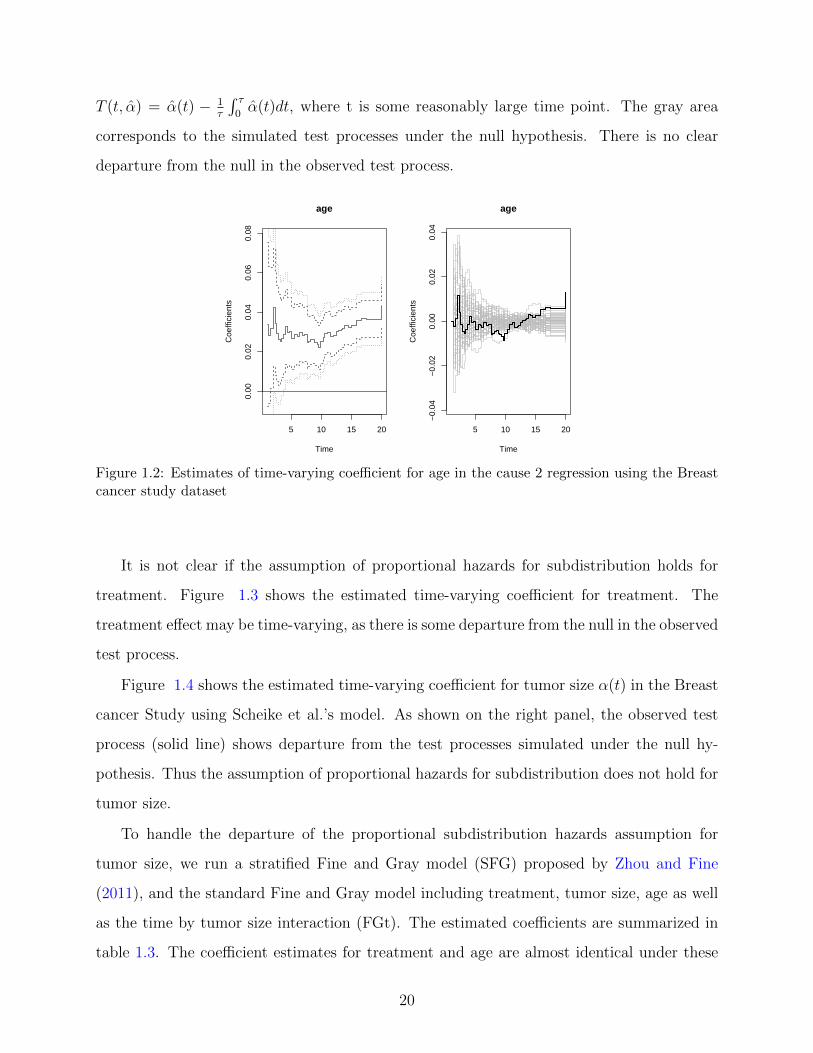
T (t, α) = α(t) − 1τ

∫ τ0α(t)dt, where t is some reasonably large time point. The gray area

corresponds to the simulated test processes under the null hypothesis. There is no clear

departure from the null in the observed test process.

5 10 15 20

0.00

0.02

0.04

0.06

0.08

Time

Coe

ffici

ents

age

5 10 15 20−

0.04

−0.

020.

000.

020.

04

Time

Coe

ffici

ents

age

Figure 1.2: Estimates of time-varying coefficient for age in the cause 2 regression using the Breastcancer study dataset

It is not clear if the assumption of proportional hazards for subdistribution holds for

treatment. Figure 1.3 shows the estimated time-varying coefficient for treatment. The

treatment effect may be time-varying, as there is some departure from the null in the observed

test process.

Figure 1.4 shows the estimated time-varying coefficient for tumor size α(t) in the Breast

cancer Study using Scheike et al.’s model. As shown on the right panel, the observed test

process (solid line) shows departure from the test processes simulated under the null hy-

pothesis. Thus the assumption of proportional hazards for subdistribution does not hold for

tumor size.

To handle the departure of the proportional subdistribution hazards assumption for

tumor size, we run a stratified Fine and Gray model (SFG) proposed by Zhou and Fine

(2011), and the standard Fine and Gray model including treatment, tumor size, age as well

as the time by tumor size interaction (FGt). The estimated coefficients are summarized in

table 1.3. The coefficient estimates for treatment and age are almost identical under these

20

0 5 10 15 20

−4−2

02

4

Time

Coeff

icients

trt

0 5 10 15 20

−20

2

Time

Coeff

icients

trt

Figure 1.3: Estimates of time-varying coefficient for treatment in the cause 2 regression using theBreast cancer study dataset

5 10 15 20

−0.

010.

000.

010.

020.

03

Time

Coe

ffici

ents

tsize

5 10 15 20

−0.

02−

0.01

0.00

0.01

0.02

Time

Coe

ffici

ents

tsize

Figure 1.4: Estimates of time-varying coefficient for tumor size in the cause 2 regression using theBreast cancer study dataset

three models.

We apply our modified logistic model and the modified Weibull model with the general-

21

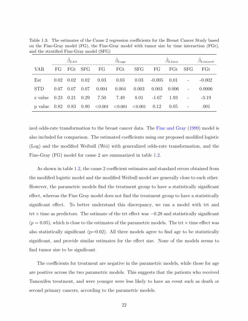
Table 1.3: The estimates of the Cause 2 regression coefficients for the Breast Cancer Study basedon the Fine-Gray model (FG), the Fine-Gray model with tumor size by time interaction (FGt),and the stratified Fine-Gray model (SFG)

β2 trt β2 age β2 tsize β2 tsize∗t

VAR FG FGt SFG FG FGt SFG FG FGt SFG FGt

Est 0.02 0.02 0.02 0.03 0.03 0.03 -0.005 0.01 - -0.002

STD 0.07 0.07 0.07 0.004 0.004 0.003 0.003 0.006 - 0.0006

z value 0.23 0.21 0.29 7.50 7.49 8.01 -1.67 1.93 - -3.19

p value 0.82 0.83 0.80 <0.001 <0.001 <0.001 0.12 0.05 - .001

ized odds-rate transformation to the breast cancer data. The Fine and Gray (1999) model is

also included for comparison. The estimated coefficients using our proposed modified logistic

(Log) and the modified Weibull (Wei) with generalized odds-rate transformation, and the

Fine-Gray (FG) model for cause 2 are summarized in table 1.2.

As shown in table 1.2, the cause 2 coefficient estimates and standard errors obtained from

the modified logistic model and the modified Weibull model are generally close to each other.

However, the parametric models find the treatment group to have a statistically significant

effect, whereas the Fine Gray model does not find the treatment group to have a statistically

significant effect. To better understand this discrepancy, we ran a model with trt and

trt× time as predictors. The estimate of the trt effect was −0.28 and statistically significant

(p = 0.05), which is close to the estimates of the parametric models. The trt× time effect was

also statistically significant (p=0.02). All three models agree to find age to be statistically

significant, and provide similar estimates for the effect size. None of the models seems to

find tumor size to be significant.

The coefficients for treatment are negative in the parametric models, while those for age

are positive across the two parametric models. This suggests that the patients who received

Tamoxifen treatment, and were younger were less likely to have an event such as death or

second primary cancers, according to the parametric models.

22

A Cox regression was run in order to better determine the effect of covariates, and par-

ticularly of the Tamoxifen treatment on the cause 2 events. The regression coefficient for

age is similar when using Cox Regression, our parametric models, and the Fine Gray model.

The regression coefficient for tumor size is not statistically significant when using Cox re-

gression, which is consistent with our parametric models, and the Fine and Gray model.

The Cox regression treatment effect is negative (-0.13) and borderline statistically signifi-

cant (p = 0.08). Our parametric models find the treatment effect to be negative (-0.3 and

-0.6) and statistically significant (p = 0.03 and p<0.01). But the Fine Gray model does not

find the treatment effect to be statistically significant (p = 0.8). When using Fine Gray with

a treatment by time effect, the estimate of the treatment effect was -0.28 and statistically

significant, and the treatment by time effect was positive and also statistically significant.

Therefore, there is some evidence showing that Tamoxifen lowers the risk of other events.

0 5 10 15 20

0.0

0.2

0.4

Years

Pro

babi

lity

PlaceboTamoxifen

Figure 1.5: Nonparametric estimates of cause 2 CIF curves for Placebo and Tamoxifen groups

On Figure 1.5, we plot nonparametric estimates of the cause 2 CIF curves for the placebo

and the Tamoxifen groups. The curve of the Tamoxifen group is below that of the placebo

group, showing a small effect of Tamoxifen on the incidence of other events.

23

1.4.3 Model Discussion

In this first part of this dissertation, we focused on the joint regression modeling of two

cumulative incidence functions under an additivity constraint. We have proposed a para-

metric regression model using a flexible baseline function and a proportional hazard or a

generalized odds rate model for covariate effects. The primary advantage of our parametric

model is that it explicitly incorporates the additivity constraint between the asymptotes of

the CIFs from the primary and secondary causes for any given covariates. Our parametric

model provides a robust alternative to its semiparametric counterparts: it not only accounts

for nonproportionality but also provides a reliable variance estimator. Furthermore, it does

not require the modeling of censoring times.

We assessed the robustness of our proposed models by considering such baseline functions

as the modified logistic and the modified Weibull. Likelihood for the modified logistic model

is 6085.6, whereas likelihood for the modified Weibull model is 6091.7. The likelihoods of

the two models are very close, so that no one of our two models seems better than the other

in this data example.

24

2.0 STATISTICAL ANALYSES OF PILL-MONITORING DATA

2.1 INTRODUCTION

The objective of this chapter is to present several analyses of data collected via an electronic

medication-event monitoring device. The device in question is a medication bottle which

records the times when it is opened.

In medication bottle opening events studies, data include event times, which are corre-

lated within individuals. The focus can be on the durations between events, the durations

between the baseline and the events, or the number or rates of events. In simple cases, the

data-generating process can be modeled by a renewal process. In more complex situations,

the events can display short term dependence, or present a between-individual dependence

structure. The wide range of data situations gives way to numerous approaches when it

comes to model specification and estimation.

There are many reasons why some patients do not follow their drug regimen. They may

forget to take their drugs. They may have difficulties managing several medications with

different dosing regimens. A patient with an asymptomatic disease, such as high blood pres-

sure or high cholesterol, may believe that the treatment is no longer needed. Patients may

skip doses or stop taking medications because of their side effects. Elderly patients may

have memory-loss or even dementia. Medical non-adherence has direct health consequences

as well as costs related to the complications of the chronic condition. For high blood pres-

sure, it could be a cerebrovascular accident; and for Type 2 diabetes, it could be heart disease.

25

Medication adherence is generally computed over some interval of time as the percentage

of correct medication administrations over the total number of prescribed administrations.

When observed in a group of subjects, the distribution of medication adherence is often J-

shaped. That is because most study participants correctly follow their medication regimen,

but some take no medication, and others miss some doses. J-shape distributions are quite

different from Gaussian distributions, so that parametric techniques utilizing a normal distri-

bution can be inadequate, especially in small sample size situations. For example, measures

of central tendency fail to provide an adequate summary of the distribution.

Summarizing and analyzing the hundreds of data points per subject which are often col-

lected in medication bottle opening events studies is challenging. Several statistics can be

used including the average or the median adherence over a given interval, often three weeks.

Some study reports provide an indicator of the spread of the distribution of adherence. This

is adequate if adherence is relatively constant within the interval, or if the changes in ad-

herence across time are not of great interest. However, patients can behave differently as

time progresses. The behavior of patients often changes as they are affected by stress and

fatigue during the week, then have time to take better care of themselves over the weekend.

If adherence rates increase or decrease within the intervals, then simple descriptive statistics

will not properly summarize the data.

One approach to analyze adherence data is to categorize the percentage of correct dose

administrations into two groups. However, some potentially significant changes occuring

across time can then go unnoticed, because the threshold is not crossed. 80% is often con-

sidered the lowest percentage of correct doses for a good adherer. A patient who progresses

from 20% to 70% adherence will be considered a poor adherer throughout the study, despite

a substantial improvement after the intervention.

A different method was developed by Rohay (2010) who used a mixture of beta distri-

26

butions to describe the distribution of the adherence of several patients. The author used

the expectation-maximization algorithm to obtain parameter and standard error estimates

of that distribution. The parameters can be used to characterize the pill taking behavior

of different groups of participants, so that this approach can be of great interest to study

investigators. On the other hand, this analysis can be computationally intensive.

As indicated by Knafl GJ (2004), another assessment of medication adherence across

time can be obtained by grouping observation days and computing counts and rates over

separate periods of cap use. To do this, the analyst divides the observation period into

intervals, counts the number of openings (or the number of adherent days in each interval),

and obtains the opening rate for the interval. The patterns of adherence can then be studied

across time using splines fitted onto the observations of number or rates of openings. The

polynomial curves are of interest for several reasons. First, power terms in the polynomial

can be added or removed from the model using the maximization of a score function. Second,

an alternative measure of the participant's adherence may be obtained by calculating the

smoothness of the polynomial fit to the participant's count data.

This part of the thesis looks at adherence data via the analysis of time between two

medication bottle openings (also called gap times). To this end, we largely focus on frailty

models. Frailty models can be used for duration data, and are characterized by the inclusion

of a random effect, that is, an unobservable random variable which represents the hetero-

geneity of observations coming from the same cluster. A cluster can be a family of several

individuals who share genetic factors, for example. In our recurrent events study, the cluster

is the individual with his or her psychosocial and behavioral characteristics.

Proportional hazards models (Cox, 1972a) were extended to frailty models (Andersen

et al., 1995; Hougaard, 1995; Sinha and Dey, 1997), which are characterized by the presence

of a random effect. Vaupel et al. (1979) presented the frailty term in the context of univari-

ate survival models, while Clayton (1978) and Oakes (1982) generalized frailty modeling to

27

multivariate survival models.

The rest of the thesis is organized as follows. We review several models for the analysis

of gap times in section 2.2. We describe the analysis of a prescription bottle event dataset

in section 2.3. An exploratory cluster analysis of survival curves is presented in section 2.4.

We indicate the directions of our future work in section 2.5.

2.2 MODELS

2.2.1 Modeling of gap times

We assume that individual i is observed over the time interval [0, τi] and that w = 0 corre-

sponds to the start of the event process. The gaps Tij between events have hazard function

λ(t|xi), where xi is a covariate. If ni events are observed at times 0 < wi1 < · · · < wini≤ τi,

let tij = wij − wi,j−1, with j = 1, . . . , ni. These are the observed gap times for individual i

with the final time being possibly censored. Let ti,ni+1 = τi − ti,ni.

The likelihood function from m independent individuals is of the form

m∏i=1

{ni∏j=1

λ(tij|xi) exp (−Λ(ti,j|xi))

}exp (−Λ(ti,ni+1|xi)) ,

where λ(tij|xi) is the hazard and Λ(ti,j|xi) is the cumulative hazard.

We now review several model formulation for the analysis of the times between medication

administrations.

28

2.2.1.1 Cox regression The Cox semiparametric multiplicative hazards model in which

the hazard function given Xi is of the form

λ(t|Xi) = λ0(t) exp(βTXi),

where λ0(t) is the baseline hazard function.

The basic assumption in Cox's proportion hazard model is that the survival time of

subjects are independent. This assumption is violated in pill monitoring studies as the

collected gap times exhibit correlation. A naive use of the Cox model in a pill monitoring

study would greatly inflate the sample size and the power of the analyses. The sample size

could erroneously be taken to be equal to the number of bottle openings. In order to use

the simple Cox model, the analyst would have to only use one observation, or one summary

measure of the observations, per study participant.

2.2.1.2 Accelerated failure time models Let T be a response time, and define Y =

log(T ). An accelerated failure time (AFT) model is of the form:

Y = β0 + x′β + σε, (2.2.1)

where x = (x1, . . . , xk)′ is a covariate vector, β = (β1, . . . , βk)

′ is a vector of regression

coefficients, σ>0 is a scale parameter, and ε is a random variable whose distribution is

independent of x. When ε has standard extreme value, logistic, and normal distributions, T

has Weibull, log-logistic, and log-normal distributions, respectively. Because of the absence

of frailty, only one observation per ID or an ID level summary measure can be used. One

approach is to average the gap times of an individual and use that mean value as a summary

measure.

2.2.1.3 Frailty models with nonparametric baseline function The heterogeneity

of the times to openings can lead to trouble insofar as parameter estimates can be inconsis-

tent, standard errors can be wrong, and estimates of duration dependency can be misleading.

29

Frailty terms seek to explicitly account for the extra variance associated with the variability

of the gap times within each prescription bottle user.

Consider a survival regression model with hazard λ(t|θ, β), where θ is a vector-valued

parameter and β is a regression parameter. Assume that the random variable U , with density

g(ui|σ2) denotes the unobservable individual frailties and that E(U) = 1 and V (U) = σ2 .

The random effect needs to be integrated out. The likelihood is:

L(θ, β, σ2) = Πni=1

∫ ∞0

λ(ti|ui, θ, β)δiS(ti|ui, θ, β)g(ui|σ2)dui,

where δi is the censoring indicator.

We can modify Cox's model into the form λij(t) = λ0(t)ui exp(xijβ) where the uis are

log-normal with a mean parameter equal to 0. Observations j within cluster i share the

frailty ui, and fail faster (hence the term frailty) than average if ui > 1.

Another way to write this frailty model is as

λij(t|bi) = λo(t) exp(xijβ + bi), where bi ∼ N (0, σ2), (2.2.2)

and where observations j are in clusters i, and bi is uncorrelated with bi′ . The spread of bi

quantifies the variability of the occurrence rate between individuals.

Therneau and Grambsch (2000) introduce an interesting model which assumes a frailty

whose distribution is gamma with parameters ( 1α, 1α

). α quantifies the amount of heterogene-

ity among subjects. If α is large, variability among individuals is high, and the values of the

variable will be close to 1. On the other hand, a small α implies low heterogeneity among

the observations individuals within the cluster.

The clustering is modeled by the random effect ξi. The gap time has intensity function

λij(t|ξi) = ξiλo(t) exp(xijβ), (2.2.3)

30

where ξi ∼ Γ(

1α, 1α

)i.i.d., E(ξi) = 1, and Var(ξi) = α. The difference between (2.2.2)

and (2.2.3) is the distribution of the random effect. The frailty term can be specified in an

additive way, as in (2.2.2), or in a multiplicative fashion, as in (2.2.3).

Instead of choosing ξi in (2.2.3) to be distributed as i.i.d. gamma random variables,

one can use for example a positive stable, an inverse gaussian, or a power variance function

distribution (Duchateau and Janssen, 2008; Wienke, 2010). While being able to choose be-

tween different frailty distributions is useful, we are going to focus on the model form with

the normal frailty, such as in (2.2.2). That model provides a simpler framework for modeling

multiple and correlated random effects.

We note that the individual frailty is modeled as an extra risk that the medication

bottle is opened. As such, the frailty is related to relative adherence. The individual frailty

measures the adherence of the individual when compared to the sample.

2.2.1.4 Modeling of the random effects As presented in Therneau and Grambsch

(2000), a more general frailty model is:

λ(t) = λ0(t)eXβ+Zb, where b ∼ G(0,Σ(θ)),

where λ0 is the baseline hazard function, X and Z are the design matrices for the fixed and

random effects, respectively, β is the vector of fixed-effects coefficients and b is the vector

of random effects coefficients. The random effects distribution G is modeled as Gaussian

with mean zero and a variance matrix Σ, which in turn depends on a vector of parameters

θ. We start with the simple model characterized by one random intercept per individual.

Z is the one-way ANOVA design matrix. Zij = 1 if gap time j is that of individual i. A

more complex model would require the individuals to be nested within a group, such as an

enrolling center, or a hospital.

We may want to test the significance of the random effects. In order to test, we fit the

model without one of the random effects and compare the integrated likelihood, which we

denote L, for the two fits. The following chi-square statistic is computed:

31

2 log(Lmodels)− 2 log(Lmodell) ∼H0 χ2(dfmodels−dfmodell) ∼ χ2

(dfs−dfl) ∼ χ2diff .

Here, s denotes the smaller model with fewer parameters, whereas l denotes the larger

model with more parameters. This χ2diff diff-value is distributed with dfdiff degrees of freedom

and can be checked for significance.

2.2.1.5 Cox frailty model with time-varying covariate Investigators are often in-

terested in studying the dynamics of time to administration as study time increases. Several

authors have pointed out that a patient's adherence decreases as the novelty feel of the

treatment and prescription bottle wears out and between clinic visits Cramer et al. (1990);

Feinstein (1990); de Klerk et al. (2003). Such a behavior is often called the “white coat”

effect.

Let TiSt denote the time a patient has been in the study, or the time a patient has been

using the prescription bottle, whichever is available from the data set. The hazard function

can be written as:

λij(t) = λ0(t) exp(xiβ + TiStijβt + bi), where bi ∼ Normal(0, σ2) . (2.2.4)

Alternately, the frailty effect can be specified as a gamma distribution:

λij(t|ξi) = ξiλo(t) exp(xiβ + TiStijβt), (2.2.5)

where ξi ∼ Γ(

1α, 1α

)i.i.d., E(ξi) = 1, and Var(ξi) = α

2.2.1.6 Frailty models with parametric baseline function We now turn to frailty

models with parametric baseline hazard functions. The frailty model is defined in terms of

the conditional hazard

λij(t|ui) = h0(t)ui exp(xijβ), (2.2.6)

32

where h0 is the baseline hazard function. Following Munda and Legrand (2012), we consider

a Weibull distribution for the baseline hazard. The Weibull hazard function is specified as

h(t; ρ, ν) = ρνtρ−1, with ρ>0 and ν>0.

Again following Munda and Legrand (2012), we set the frailty term to be a gamma

random variable U with probability density function:

f(u; θ) =u1/θ−1 exp(−u/θ)

Γ(1/θ)θ1/θ, θ>0.

The variance of the frailty term U is θ.

2.2.2 Counting processes

The focus in this section is to analyze counts of bottle events within a particular window

of time, rather than gap times. Let i = 1 . . . n note independent subjects. Ni(t) counts the

number of events for the period of time [0, τi], for subject i.

An interesting quantity is the mean cumulative function (MCF) of the number of medi-

cations taken by the patients. The MCF is a staircase function that depicts the cumulative

number of medication administrations over time. The cumulative mean function provides

a graphical representation of the degree of medication adherence for each patient. It can

be used to compare the compliance of two of more patients. Furthermore, the cumulative

mean function can be estimated for groups of patients, thus enabling group comparisons. To

our knowledge, the MCF has not been used to represent or analyze medication adherence

datasets.

2.2.2.1 Bayesian estimation of Cox regression with random effects Following

Nielsen et al. (1992), we formulate the frailty model using the counting process notation.

For subjects i = 1, . . . , n, we observe processes Ni(t) which count the number of events which

33

have occurred up to time t. The corresponding intensity process Ii(t) is given by

Ii(t)dt = E(dNi(t)|Ft−),

where Ft is a filtration.

We model the clustering of gap times within patients by introducing a frailty term into

the proportional hazards model. In counting process notation, this gives

Ii(t)dt = Yi(t) exp(βxi + bi)dΛ0(t), where, bi ∼ Normal(0, 1/θ) .

We observe dataD = (Ni(t), Yi(t), xi), i = 1, . . . , n and parameters β, Λ0(t) =∫ t

0λ0(u)du

is to be estimated non-parametrically. The joint posterior distribution of the model is defined

by

P (β,Λ0()|D) ∼ P (D|β,Λ0())× P (β)× P (Λ0()).

A non-informative gamma prior can be assumed for θ, the precision of the frailty parame-

ters. To our knowledge, the Bayesian frailty model has not been used to analyze prescription

bottle events datasets.

2.2.3 Software

The Cox model is handled by the functions of package coxph in R. The survreg function in

package survival can fit an accelerated failure time model.

Frailty models can be handled by packages coxph, frailtypack, parfm, and coxme in

R. Coxph can fit frailty models with a random effect drawn from a gamma distribution.

In frailtypack, a random effect, and a random slope can be fitted. The random effects

can be gamma or log-normal. The baseline function λ0(T ) can be semiparametric, piecewise

constant, or parametric Weibull. In addition, frailtypack allows the analyst to compare

the AIC from different model specifications to determine the best fit for the data. Pack-

age parfm fits frailty models with parametric baseline hazard functions. Possible baseline

34

hazards are Weibull, inverse Weibull, exponential, Gompertz, log-normal and log-logistic.

Possible frailty distributions are gamma, inverse Gaussian, positive stable and log-normal.

Coxme allows the analyst to compare the AIC from different model specifications to deter-

mine the best fit for the data.

SAS's proc reliability provides the mean cumulative function, as well as confidence in-

tervals. Regression analyses for recurring events data sets can also be run via SAS's proc

reliability. Bayesian Cox regression models can be handled by BUGS.

2.3 ANALYSIS OF DATA

This section applies frailty models to the data set of the Evaluation of Adherence Interven-

tions in Clinical Trials (NIH-HL48992) study, a randomized controlled trial which we refer

to as the ACT study. The ACT Study recruited 180 adults. The participants were given

their medication in Medication Event Monitoring System (MEMS)-capped bottles contain-

ing a computer chip, which records each time the prescription bottle is opened. All subjects

had a prescribed regimen of 1 dose/day. The cap opening times recorded were presumed to

coincide with medication-taking.

The ACT study was nested within the Effect of Cholesterol Lowering on Behavior (or

CARE) study (NIH-HL46328), a gender-balanced, randomized, controlled trial, where the

180 subjects were randomized either to a lipid lowering drug (90 subjects), or to a placebo (90

subjects). The participants of the CARE study continued into the ACT study, where they

were randomized to one of three groups: controls, habit training, or habit training/problem

solving. The behavioral training delivered to the habit training, and to the habit train-

ing/problem solving subjects aimed to improve their medication adherence. All subjects

were prescribed a once-a-day medication regimen. There were 59 subjects in the controls

35

group, 63 in the habit training group, and 58 in the habit training/problem solving group.

Data were collected over a six month period. Available variables include electronically

monitored events (MEMs), published self-report inventories (Morisky, Shea, Haynes), spe-

cific recall over one day, one week, one month, and six months, as well as pill counts.

Overall, the sample was evenly distributed by gender (53.4% male), predominantly white

(87.8%), and middle-aged (mean age=46.2 years). Most subjects (68.2%) were married, and

75.4% of the subjects were employed full or part time. The subjects were well-educated,

with 98.9% of them having a high school diploma/GED or more education.

The missingness rate is very low in the sociodemographic, and electronic event monitor-

ing variables. No data inconsistencies are detected. The length of use of the MEMS caps

ranges between 0 and 9.5 months, with an average of 6.0 months, and a standard deviation

of 1.4 months. Summary adherence is computed as the ratio of the number of openings over

the number of days observed. When the number of medication administrations is greater

than the number of days, the computed adherence is higher than 1. Summary adherence

ranges between 0.02 doses per day and 1.44 doses per day, with a median of 0.99 doses per

day and an interquartile range of 0.31 doses per day.

2.3.1 Exploratory data analysis

The histogram of the gap times across all the observations of all the subjects is in Figure 2.1.

The time unit of interest is hours. The distribution of the gap times shows a protuberance

between 0 and 3 hours, a very high spike around 24 hours, and two bumps of decreasing

sizes around 48 and 72 hours. The distribution of the gap times does not seem to lend itself

to simple parametric modeling. The histogram of the log gap times, shown in Figure 2.2,

appears to be that of a mixture of several time distributions. From that standpoint, the

nonparametric baseline hazard approach is appealing.

36

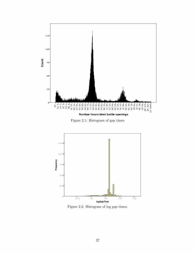
Figure 2.1: Histogram of gap times

logGapTime

7.505.002.50.00-2.50

Fre

qu

en

cy

12,500

10,000

7,500

5,000

2,500

0

Figure 2.2: Histogram of log gap times.

37

We plot individual survival curves of gap times in figures 2.3 and 2.4. These curves

show various pill-taking behaviors. ID 1328's gap time survival curve drops from around

.98 to around 0.05 very steeply around 24 hours. ID 1328 is thus very good at taking their

medication with a gap time consistently around 23 to 24 hours.

ID 1517's gap time survival curve shows several drops between time 0 and 72 hours. A

relatively small drop before time 2 hours shows that the medication bottle was opened several

times in the space of a couple of hours. This is not consistent with a once-a-day medication

regimen. Perhaps the participant forgot they had already taken their medication, or was

experimenting with the prescription bottle, or the participant was pocketing the dose for the

next day. A fairly large drop of the survival curve is seen around 24 hours, consistent with

the subject opening the bottle once-a-day for some of the days of the experiment. Another

small drop of the survival curve around 48 hours shows that the subject forgot their medi-

cation some of the days, or was taking the medication they had pocketed. Another smaller

drop around 72 hours shows that the bottle was not opened for a duration of 3 days for some

part of the experiment.

Gaptime

80.0060.0040.0020.00.00

Cu

m S

urv

iva

l

1.0

0.8

0.6

0.4

0.2

0.0

Survival Function

Figure 2.3: ID 1328's individual survival curve.

38

Gaptime

80.0060.0040.0020.00.00

Cu

m S

urv

ival

1.0

0.8

0.6

0.4

0.2

0.0

Survival Function

Figure 2.4: ID 1517's individual survival curve.

Figure 2.5 shows the survival curve of the entire sample. The survival curve shows a slow

decrease during the first 24 hours, indicating that some patients will open their prescription

bottle in the first 24 hours after their previous medication administration. The survival curve

then shows a large and steep drop around 24 hours. This indicates that patients tend to

have the habit of taking their medication around the same time of the day. Perhaps around

breakfast time, lunch, or possibly bedtime.

The survival curve shows a smaller, but steep drop around 48 hours. This indicates that

some patients will forget their dose the first day, but then successfully take their medication

at their usual time of the day on the second day. A much smaller drop is seen around 72

hours. This indicates that some patients will forget their dose on both the first and second

day, but then successfully take their medication at their usual time of the day on the third

day. Those patterns can also be seen on the hazard plots.

39

0 20 40 60 80 100

0.0

0.2

0.4

0.6

0.8

1.0

hours between med administration

Sur

viva

l

Figure 2.5: Survival curve for the entire sample

2.3.2 Proportional hazard assumption

We plot the Kaplan-Meier survival curves for each gender in order to check the proportional

hazard assumption. The plots are shown in figure 2.6. The female survival curve is for

the most part above the male survival curve by a small distance which is about the same

throughout time. Therefore the proportional hazard assumption seems to hold for gender.

2.3.3 Model comparison and covariate selection

Tables 2.1 and 2.2 show the results of analyses run using parametric and nonparametric

models. Gender is found to be statistically significant or to approach significance in all

models. The intensity function of the frailty models is higher for male participants, rela-

tive to female participants, indicating that the time between medication administrations is

longer for females. The accelerated failure time model is run using individual-level average

gap times, so that the effect of the time spent in study cannot be assessed. Time in study

40

Gaptime

80.0060.0040.0020.00.00

Cu

m S

urv

iva

l

1.0

0.8

0.6

0.4

0.2

0.0

Survival Functions

Female

Male

Sex

Figure 2.6: Survival curves by gender.

was calculated in months. The three frailty models (2.2.6), (2.2.4), and (2.2.5) find time in

study to be statistically significant. The regression coefficient for Time in study is negative,

indicating that as Time in Study passes, intensity goes down, and thus the time between

medication administrations increase.

2.3.4 Interpretation of the random effect

In this section, we focus on models which use Gaussian distributed frailties. The “frailty” of

subject k can be interpreted as an excess noncompliance fk = exp(bk) in taking medication

for individual k. The random individual effect in our model has a standard deviation of .30.

We can expect about 15% of the subjects to be 1 standard deviation below the mean, and

these individuals will have a noncompliance that is exp(1 × .30) = exp(.30) = 1.35 greater

than the norm. This is a modestly large individual effect.

41

We obtain estimates of the frailties for all the subjects. The lowest frailty is -1.0, the

highest is 0.46, and the mean is 0. In the context of this adherence study, low frailties

indicate subjects with longer gap times and thus poorer adherence behavior. ID1139 whose

survival curve is shown in figure 2.7 is a poor adherer whose gap time distribution has a long

right tail (skewness=3.2). The mean gap time (72 hours) and the 75% percentile (50.4 hours)

of subject 1139 are high. The frailty of ID1139 is very low (-0.73). In contrast, consider

ID1328 whose survival curve is shown in figure 2.3. Subject 1328 is a high adherer with a

mean gap time of 24.6 hours. The frailty of ID1328 is 0.25. Frailty estimates can therefore

help characterize the pill-taking behavior of subjects. They can also be useful during the

screening phase of a study. Frailty estimates can help identify poor adherers, and those

subjects are more susceptible to respond to the help of interventionists.

Gaptime

600.00400.00200.00.00

Cu

m S

urv

ival

1.0

0.8

0.6

0.4

0.2

0.0

Survival Function

Figure 2.7: ID 1139's individual survival curve.

Confidence intervals for the random effect can be obtained from a profile likelihood. We

start by computing the likelihood over a range of values for the variance. The 95% profile

likelihood confidence interval is the region where the curve lies above the line, i.e., the set of

values x for which a 1 degree of freedom likelihood ratio test would not reject the hypoth-

42

esis that the true standard deviation = x. We get the following estimate of the confidence

interval: from .27 to .35.

0.25 0.30 0.35 0.40

870

875

880

Standard deviation of the random effect

2 *

logl

ik

Figure 2.8: Profile likelihood for the individual random effect model

We estimate a model containing a random individual effect nested within a random treat-

ment effect. The difference on the likelihood brought about by the treatment effect is very

small and we conclude that the random treatment effect is not statistically significant.

43

Table 2.1: Parametric models

Type of model Accelerated Failure Time Frailty model

Baseline hazard No baseline hazard Weibull

Frailty details No frailty gamma

Equation (2.2.1) (2.2.6)

r package survival parfm

Fixed effect parameters Est. (SE) p Est. (SE) p

β male -0.21 (.08) .01 0.18 (0.12) 0.06

β Tstudy - - -0.03 (3.0E-3) < .01

Frailty Parameter

θ - 0.37

Baseline hazard

Parameters

ρ - 1.47

ν - 0.007

Log-likelihood -107133 -96330

44

Table 2.2: Frailty models with non parametric baseline hazard

Type of model Fraily model Frailty model

Equation (2.2.5) (2.2.4)

Baseline Nonparametric Nonparametric

hazard

Frailty gamma Gaussian

r package frailtypack coxme

Fixed effect Est. (SE) p Est. (SE) p

Parameters

β male 0.15 (0.08) 0.05 0.15 (0.05) <.01

β Tstudy -0.03 (3.5E-3) <.01 -0.02 (3.4E-3) <.01

Frailty

Parameters

α 0.19 (0.025) -

σ2 - 0.09

Likelihood -228439 -225609

45

2.3.5 Model validation

In figure 2.9 we plot the survival functions for the gap times at the beginning and at

the end of the observation period. The gap times at the beginning of the study, when the

participants met with the nurse and the study manager, were shorter than the last gap times.

Figure 2.9: Survival curves of first and last gap times

46

2.4 EXPLORATORY CLUSTER ANALYSIS

The goal of this section is to cluster the survival curves of the participants into a small

number of curves representing groups of patients. We use a two-stage approach. In the first

step we reduce the dimension of the survival curves using spline regression. In the second

step we cluster the curves according to the spline coefficients.

2.4.1 Spline regression

We have knots (t1, . . . , tn) and a vector of responses (y1, . . . , yn). We start by considering g

a function consisting of piecewise polynomials. We can put constraints on the behavior of

the function g at the break points.

We can write any function g in the truncated basis power:

g(x) = θ0,1 + θ0,2x+ · · ·+ θ0,kxk−1 +

...

θi,1(x− ti)0+ + θi,2(x− ti)1

+ + · · ·+ θi,k(x− ti)k−1+ +

...

θm,1(x− tm)0+ + θm,2(x− tm)1

+ + · · ·+ θm,k(x− tm)k−1+

where (·)+ = max(·, 0).

(x − ti)+ is sometimes called a hinge function. (x − ti)k−1+ is a shifted power function

that is truncated to the left of ti.

2.4.1.1 Cubic splines Cubic splines are continuous and have continuous first and second

derivatives. In this case we can write:

g(x) = θ0,1 + θ0,2x+ · · ·+ θ0,4x3 + θ1,k(x− t1)3 + · · ·+ θm,k(x− tm)3

47

2.4.1.2 Natural smoothing splines Natural splines add the constraint that the func-

tion must be linear after the knots at the end points. This forces two more restrictions

since g′′ must be 0 at the end points. Among all functions g with two continuous first two

derivatives, find one that minimizes the penalized residual sum of squares

n∑i=1

{yi − g(ti)}2 + λ

∫ b

a

{g′′(t)}2 dt

where λ is a fixed constant, and a ≤ t1 ≤ · · · ≤ tn ≤ b.

2.4.2 Application to the ACT/CARE study dataset

2.4.2.1 Clustering using ID-level summary measure This approach is simple to

implement and its results can be compared to other clustering methods. Given a set of

observations (x1, x2, . . . , xn), where each observation is a d-dimensional real vector, k-means

clustering aims to partition the n observations into k (≤ n) sets S = {S1, S2, . . . , Sk} so as

to minimize the within-cluster sum of squares (WCSS). In other words, its objective is to

find:

arg minS

k∑i=1

∑x∈Si

‖x− µi‖2

where µi is the mean of points in Si.

The percentage of gap times that lie between 21 and 27 hours are calculated. Also

computed are the percentage of gap times that were greater than 27 hours. Using k-means

Clustering analysis on those two ID-level summary measures, and having indicated 4 clus-

ters, we get the following plot.

The participants of the blue group (about 6%) are low adherers: the prescription bottle

openings in this group are not very frequent when compared to the openings of the other

three groups of participants. The patients seem to have a hard time taking their medication

at the same time of the day: the survival curve drops around 24 and 48 hours are very small.

There does not seem to be a time pattern when it comes to the openings. Those happen at

48

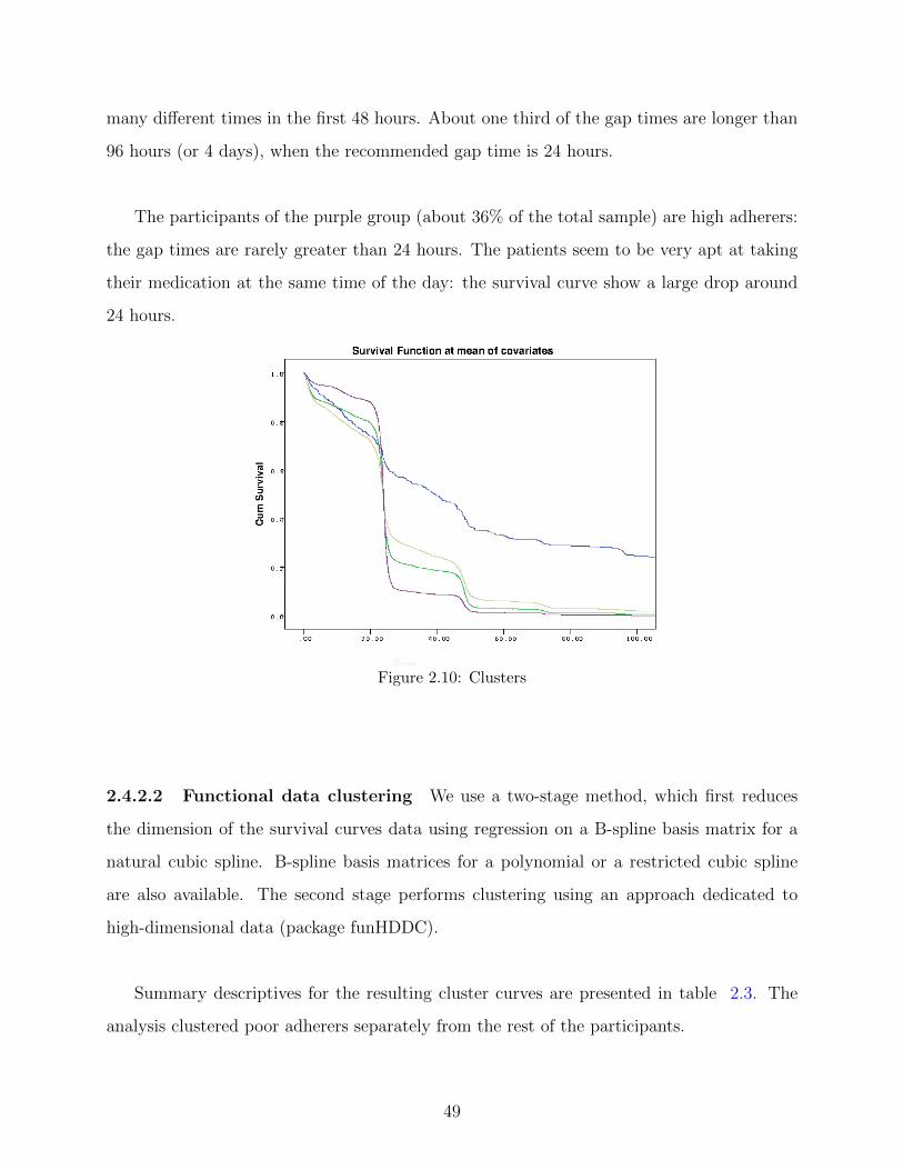
many different times in the first 48 hours. About one third of the gap times are longer than

96 hours (or 4 days), when the recommended gap time is 24 hours.

The participants of the purple group (about 36% of the total sample) are high adherers:

the gap times are rarely greater than 24 hours. The patients seem to be very apt at taking

their medication at the same time of the day: the survival curve show a large drop around

24 hours.

Figure 2.10: Clusters

2.4.2.2 Functional data clustering We use a two-stage method, which first reduces

the dimension of the survival curves data using regression on a B-spline basis matrix for a

natural cubic spline. B-spline basis matrices for a polynomial or a restricted cubic spline

are also available. The second stage performs clustering using an approach dedicated to

high-dimensional data (package funHDDC).

Summary descriptives for the resulting cluster curves are presented in table 2.3. The

analysis clustered poor adherers separately from the rest of the participants.

49

Figure 2.11: Individual survival curve with spline

Table 2.3: Descriptive statistics of clusters

Cluster number N Pct of gap times

lying between 21

and 27 hours

Pct female Mean age

% % years

1 103 49.9 39.8 46

2 21 31.0 76.2 44

3 51 75.4 49.0 48

4 1 0 100 39

2.5 CONCLUSION AND FUTURE WORK

In this second part of the thesis, we focused on the modeling of medication bottle opening

data. We reviewed several models, and largely focused on frailty models. These models

50

provide an important framework for adherence analyses. In chapter 2.2, we focused on

models where the clustering within individuals is accounted for by a gamma or a lognormal

variable. We discussed the interpretation of the random effect of a subject, and how it can

help characterize the adherence of that individual relative to that of the other subjects. In

chapter 2.3, we analyzed a prescription bottle opening data set. We showed that gap time

frailty models can be utilized to identify poor adherers. We evaluated the effects of several

covariates on the gap times, and found gender to be a statistically significant predictor. We

also uncovered a time effect. In chapter 2.4, we clustered the survival curves of the partici-

pants into a small number of curves representing groups of patients. The exploratory cluster

analysis focuses on the shape of the survival curves, and is useful to identify and quantify

different pill-taking behaviors.

In future work, we will apply frailty models to more prescription bottle opening events

data sets. In many adherence studies, different subjects are on different drug regimens, such

as once, twice, three times per day, or every other day, rendering the analysis of data sets

more challenging. Furthermore, we will assess the effects of more predictors on the times

between the administration of doses. Possible predictors of adherence can include sociodemo-

graphic variables, number of comorbidities, mood (anxiety, depression), perceived adherence

(self- reported adherence), and the perception of illness. Other predictors such as economic

hardship and symptom distress could also be investigated. Developing such models will be

very useful for understanding how patient-related and medication-related variables affect

individual adherence.

One limitation of the current approach is that the frailty models we considered use a

proportional hazards transformation. The proportional hazard assumption may not hold for

some covariates. Therefore, implementing a more flexible class of link functions would be

very useful.

51

3.0 BIBLIOGRAPHY

Andersen, P. K., O. Borgan, R. D. Gill, and N. Keiding (1995, June). Statistical Models

Based on Counting Processes (Corrected ed.). Springer Series in Statistics. Springer.

Beyersmann, J., A. Allignol, and M. Schumacher (2012). Competing risks and multistate

models with R. New York: Springer.

Cheng, Y. (2009). Modeling cumulative incidences of dementia and dementia-free death

using a novel three-parameter logistic function. The International Journal of Biostatistics.

Clayton, D. G. (1978, April). A model for association in bivariate life tables and its

application in epidemiological studies of familial tendency in chronic disease incidence.

Biometrika 65 (1), 141–151.

Cox, D. R. (1972a). Regression Models and Life-Tables. Journal of the Royal Statistical

Society. Series B (Methodological) 34 (2), 187–220.

Cox, D. R. (1972b). Regression models and life-tables (with discussion). Journal of the Royal

Statistical Society, Series B: Methodological 34, 187–220.

Cramer, J. A., R. D. Scheyer, and R. H. Mattson (1990). Compliance declines between clinic

visits. Archives of internal medicine 150 (7), 1509.

Dabrowska, D. M. and A. Doksum, K (1998). Estimation and testing in a two-sample

generalized odds-rate model. Journal of the american statistical association 83, 744–749.

de Klerk, E., D. van der Heijde, R. Landewe, H. van der Tempel, J. Urquhart, and S. van der

52

Linden (2003). Patient compliance in rheumatoid arthritis, polymyalgia rheumatica, and

gout. The Journal of rheumatology 30 (1), 44–54.

Doll, R. (1971). The age distribution of cancer: implications for models of carcinogenesis.

Journal of the Royal Statistical Society. Series A (General), 133–166.

Duchateau, L. and P. Janssen (2008). The Frailty Model. New York: Springer.

Feinstein, A. R. (1990). On white-coat effects and the electronic monitoring of compliance.

Archives of Internal Medicine 150 (7), 1377–1378.

Fine, J. P. (2001). Regression modeling of competing crude failure probabilities. Biostatistics

(Oxford) 2 (1), 85–97.

Fine, J. P. and R. J. Gray (1999). A proportional hazards model for the subdistribution of

a competing risk. Journal of the American Statistical Association 94, 496–509.

Gaynor, J. J., E. J. Feuer, C. C. Tan, D. H. Wu, C. R. Little, D. J. Straus, B. D. Clarkson,

and M. F. Brennan (1993). On the use of cause-specific failure and conditional failure

probabilities: Examples from clinical oncology data. Journal of the American Statistical

Association 88, 400–409.

Gooley, T. A., W. Leisenring, J. Crowley, and B. E. Storer (1999). Estimation of failure

probabilities in the presence of competing risks: New representations of old estimators.

Statistics in Medicine 18, 695–706.

Hougaard, P. (1995, September). Frailty models for survival data. Lifetime Data Analy-

sis 1 (3), 255–273.

Jeong, J. and J. P. Fine (2006). Direct parametric inference for the cumulative incidence

function. Journal of the Royal Statistical Society, Series C: Applied Statistics 55, 187–200.

Jeong, J. and J. P. Fine (2007). Parametric regression on cumulative incidence function.

Biostatistics 55, 184–200.

53

Jin, Z., D. Y. Lin, L. J. Wei, and Z. Ying (2003). Rank-based inference for the accelerated

failure time model. Biometrika 90 (2), 341–353.

Kalbfleisch, J. D. and R. L. Prentice (2002). The Statistical Analysis of Failure Time Data.

New York: Wiley.

Klein, J. P. and M. L. Moeschberger (2003). Survival Analysis: Techniques for Censored and

Truncated Data. New York: Springer-Verlag Inc.

Knafl GJ, F. K. (2004). Electronic monitoring device event modelling on an individual-

subject basis using adaptive poisson regression. Statistics in medicine 23(5), 783–801.

Munda, M. and C. Legrand (2012). parfm: Parametric frailty models in r. Journal of

Statistical Software 51 (11).

Nielsen, G., R. Gill, and A. P. (1992). A counting process approach to maximum likelihood

estimation in frailty models. Scandinavian Journal of Statistics 19 (1), 25–43.

Oakes, D. (1982). A model for association in bivariate survival data. Journal of the Royal

Statistical Society. Series B (Methodological) 44 (3), pp. 414–422.

Pepe, M. S. (1991). Inference for events with dependent risks in multiple endpoint studies.

Journal of the American Statistical Association 86 (415), 770–778.

Prentice, R. L., J. D. Kalbfleisch, A. V. Peterson, N. Flournoy, V. T. Farewell, and N. E.

Breslow (1978). The analysis of failure time data in the presence of competing risks.

Biometrics 12, 737–751.

Rohay, J. (2010). Statistical Assessment of Medication Adherence Data: A Technique to

Analyze the J-Shaped Curve. Ph. D. thesis, University of Pittsburgh.

Scheike, T. H. and M.-J. Zhang (2011). Analyzing competing risk data using the r timereg

package. Journal of Statistical Software 38 (2), 1–15.

54

Scheike, T. H., M.-J. Zhang, and T. A. Gerds (2008). Predicting cumulative incidence

probability by direct binomial regression. Biometrika 95 (1), 205–220.

Shi, H., Y. Cheng, and J. J.-H. (2013). Constrained parametric model for simultaneous

inference of two cumulative incidence functions. Biometrical Journal 55, 82–96.

Sinha, D. and D. K. Dey (1997). Semiparametric bayesian analysis of survival data. Journal

of the American Statistical Association 92 (439), 1195–1212.

Therneau, T. M. and P. M. Grambsch (2000). Modeling Survival Data: Extending the Cox

Model. New York: Springer.

Tukey, J. W. (1979a). Oxford Handbook of Innovation. New York: Academic Press.

Tukey, J. W. (1979b). Robustness in Statistics, Chapter Robust techniques for the user, pp.

103–106. New York: Academic Press.

Vaupel, J. W., K. G. Manton, and E. Stallard (1979, August). The impact of heterogeneity

in individual frailty on the dynamics of mortality. Demography 16 (3), 439–454.

Wei, L. J., Z. Ying, and D. Y. Lin (1990). Linear regression analysis of censored survival

data based on rank tests. Biometrika 77, 845–851.

Wienke, A. (2010). Frailty Models in Survival Analysis. Chapman and Hall/CRC.

Zhou, B., L. A. and J. Fine (2011). Competing risks regression for stratified data. Biomet-

rics 67 (2), 661–670.

55