chapter 3 112wahed/teaching/2083/fall09/lecture409.pdf · 2009-09-29 · bios 2083 linear models c...

BIOS 2083 Linear Models c©Abdus S. Wahed

Chapter 3 112

Chapter 4

General linear model: the least

squares problem

4.1 Least squares (LS) problem

As observed in Chapter 1, any linear model can be expressed in the

form

Y⎛⎜⎜⎜⎜⎜⎜⎜⎝

Y1

Y2

· · ·Yn

⎞⎟⎟⎟⎟⎟⎟⎟⎠

=

X⎡⎢⎢⎢⎢⎢⎢⎢⎣

x11 x12 . . . x1p

x21 x22 . . . x2p

... ... ... ...

xn1 xn2 . . . xnp

⎤⎥⎥⎥⎥⎥⎥⎥⎦

β⎛⎜⎜⎜⎜⎜⎜⎜⎝

β1

β2

· · ·βp

⎞⎟⎟⎟⎟⎟⎟⎟⎠

+

ε⎛⎜⎜⎜⎜⎜⎜⎜⎝

ε1

ε2

· · ·εn

⎞⎟⎟⎟⎟⎟⎟⎟⎠

. (4.1.1)

113


Usually X is a matrix of known constants representing the values of

covariates, and Y is the vector of response and ε is an error vector

with the assumption that E(ε|X) = 0.

The goal is to find a value of β for which Xβ is a “close” approxi-

mation of Y. In statistical terms, one would like to estimate β such

that the “distance” between Y and Xβ is minimum. One form of

distance in real vector spaces is given by the length of the difference

between two vectors Y and Xβ, namely,

‖Y − Xβ‖2 = (Y − Xβ)T (Y − Xβ). (4.1.2)

Note that for a given β, both Y and Xβ are vectors in Rn. In

addition, Xβ is always a member of C(X). Thus, for given Y and

X, the least squares problem can be characterized as a restricted

minimization problem:

Minimize ‖Y − Xβ‖2 over β ∈ Rn.

Or equivalently,

Minimize ‖Y − θ‖2 over θ ∈ C(X).

Chapter 4 114


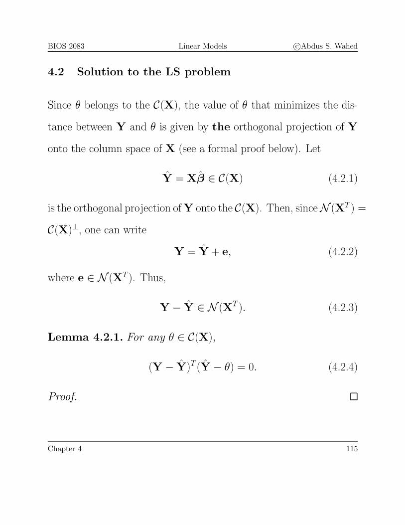
4.2 Solution to the LS problem

Since θ belongs to the C(X), the value of θ that minimizes the dis-

tance between Y and θ is given by the orthogonal projection of Y

onto the column space of X (see a formal proof below). Let

Y = Xβ ∈ C(X) (4.2.1)

is the orthogonal projection of Y onto the C(X). Then, sinceN (XT ) =

C(X)⊥, one can write

Y = Y + e, (4.2.2)

where e ∈ N (XT ). Thus,

Y − Y ∈ N (XT ). (4.2.3)

Lemma 4.2.1. For any θ ∈ C(X),

(Y − Y)T (Y − θ) = 0. (4.2.4)

Proof.

Chapter 4 115


Lemma 4.2.2. ‖Y − θ‖2 is minimized when θ = Y.

Proof.

‖Y − θ‖2 = (Y − θ)T (Y − θ)

= (Y − Y + (Y − θ))T (Y − Y + (Y − θ))

= (Y − Y)T (Y − Y) + (Y − θ)T (Y − θ)

= ‖Y − Y‖2 + ‖Y − θ‖2, (4.2.5)

which is minimized when θ = Y.

Thus, we have figured out that ‖Y − Xβ‖2 is minimum when

β = β is such that Y = Xβ is the orthogonal projection of Y

onto the column space of X. But how do we find the orthogonal

projection?

Chapter 4 116


Normal equations

Notice from our discussion on the Page 110 that

Y − Y ∈ N (XT )

=⇒ XT (Y − Y) = 0

=⇒ XT (Y − Xβ) = 0

=⇒ XTY = XTXβ (4.2.6)

Equation (4.2.6) is referred to as normal equations; solution of which,

if exists will lead us to the orthogonal projection.

Example 4.2.3. Example 1.1.3 (continued). The linear model

in matrix form can be written as

Y︷︸︸︷⎛⎜⎜⎜⎜⎜⎜⎜⎝

Y1

Y2

· · ·Yn

⎞⎟⎟⎟⎟⎟⎟⎟⎠

=

X︷︸︸︷⎡⎢⎢⎢⎢⎢⎢⎢⎣

1 w1

1 w2

... ...

1 wn

⎤⎥⎥⎥⎥⎥⎥⎥⎦

β︷︸︸︷⎛⎝ α

β

⎞⎠+

ε︷︸︸︷⎛⎜⎜⎜⎜⎜⎜⎜⎝

ε1

ε2

· · ·εn

⎞⎟⎟⎟⎟⎟⎟⎟⎠

. (4.2.7)

Chapter 4 117


Here,

XTX =

⎡⎣ n

∑wi∑

wi

∑w2

i

⎤⎦ , (4.2.8)

and

XTY =

⎛⎝ ∑

Yi∑wiYi

⎞⎠ (4.2.9)

The normal equations are then calculated as

αn + β∑

wi =∑

Yi

α∑

wi + β∑

wiYi =∑

wiYi

⎫⎬⎭ (4.2.10)

From the linear regression course, you know that, the solution to

these normal equations is given by

β =∑

(wi−w)(Yi−Y )∑(wi−w)2

α = Y − βw,

⎫⎬⎭ (4.2.11)

provided∑

(wi − w)2 > 0.

Chapter 4 118


Example 4.2.4. Example 1.1.7 (continued). The linear model

in matrix form can be written as

Y︷︸︸︷⎛⎜⎜⎜⎜⎜⎜⎜⎝

Y1

Y2

· · ·Ya

⎞⎟⎟⎟⎟⎟⎟⎟⎠

=

X︷︸︸︷⎡⎢⎢⎢⎢⎢⎢⎢⎣

1n1 1n1 0n1 . . . 0n1

1n2 0n2 1n2 . . . 0n2

... ... ... ... ...

1na 0na 0na . . . 1na

⎤⎥⎥⎥⎥⎥⎥⎥⎦

β︷︸︸︷⎛⎜⎜⎜⎜⎜⎜⎜⎜⎜⎜⎝

μ

α1

α2

...

αa

⎞⎟⎟⎟⎟⎟⎟⎟⎟⎟⎟⎠

+

ε︷︸︸︷⎛⎜⎜⎜⎜⎜⎜⎜⎝

ε1

ε2

· · ·εa

⎞⎟⎟⎟⎟⎟⎟⎟⎠

,

(4.2.12)

where Yi = (Yi1, Yi2, . . . , Yini)T and εi = (εi1, εi2, . . . , εini

)T for i =

1, 2, . . . , a. Here,

XTX =

⎡⎢⎢⎢⎢⎢⎢⎢⎣

n n1 n2 . . . na

n1 n1 0 . . . 0

... ... ... ... ...

na 0 0 . . . na

⎤⎥⎥⎥⎥⎥⎥⎥⎦

, (4.2.13)

Chapter 4 119


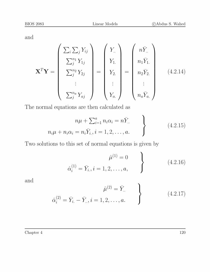
and

XTY =

⎛⎜⎜⎜⎜⎜⎜⎜⎜⎜⎜⎝

∑i

∑j Yij∑n1

j Y1j∑n2j Y2j

...∑naj Yaj

⎞⎟⎟⎟⎟⎟⎟⎟⎟⎟⎟⎠

=

⎛⎜⎜⎜⎜⎜⎜⎜⎜⎜⎜⎝

Y..

Y1.

Y2.

...

Ya.

⎞⎟⎟⎟⎟⎟⎟⎟⎟⎟⎟⎠

=

⎛⎜⎜⎜⎜⎜⎜⎜⎜⎜⎜⎝

nY..

n1Y1.

n2Y2.

...

naYa.

⎞⎟⎟⎟⎟⎟⎟⎟⎟⎟⎟⎠

(4.2.14)

The normal equations are then calculated as

nμ +∑a

i=1 niαi = nY..

niμ + niαi = niYi., i = 1, 2, . . . , a.

⎫⎬⎭ (4.2.15)

Two solutions to this set of normal equations is given by

μ(1) = 0

α(1)i = Yi., i = 1, 2, . . . , a,

⎫⎬⎭ (4.2.16)

and

μ(2) = Y..

α(2)i = Yi. − Y.., i = 1, 2, . . . , a.

⎫⎬⎭ (4.2.17)

Chapter 4 120


Solutions to the normal equations

In Example 4.2.3, the normal equations have a unique solutions,

whereas in Example 4.2.4, there are more than one (in fact, infinitely

many) solutions. Are normal equations always consistent? If we

closely look at the normal equations (4.2.6)

XTXβ = XTY, (4.2.18)

we see that if XTX is non-singular, then there exists a unique

solution to the normal equations, namely,

β = (XTX)−1XTY, (4.2.19)

which is the case for the simple linear regression in Example 4.2.3,

or more generally for any linear regression problem (multiple, poly-

nomial).

Chapter 4 121


Theorem 4.2.5. Normal equations (4.2.6) are always consis-

tent.

Proof. From Chapter 2, Page 63, a system of equations Ax = b is

consistent iff b ∈ C(A). Thus, in our case, we need to show that,

XTY ∈ C(XTX). (4.2.20)

Now, XTY ∈ C(XT ). If we can show that C(XT ) ⊆ C(XTX), then

the result is established. Let us look at the following lemma first:

Lemma 4.2.6. N (XTX) = N (X).

Proof. . If a ∈ N (XTX), then

XTXa = 0 =⇒ aTXTXa = 0

=⇒ ‖Xa‖2 = 0 =⇒ Xa = 0

=⇒ a ∈ N (X). (4.2.21)

On the other hand, if a ∈ N (X), then Xa = 0, and hence

XTXa = 0 which implies that a ∈ N (XTX), which completes

the proof.

Chapter 4 122


Now, from the above lemma, and from the result stated in chapter

2, page 53, and Theorem 2.3.2,

N⊥(XTX) = N⊥(X)

=⇒ C(XTX) = C(XT ), (4.2.22)

which completes the proof.

Least squares estimator

The above theorem shows that the normal equations are always con-

sistent. Using a g-inverse of XTX, we can write out all possible

solutions of the normal equations. Namely,

β = (XTX)gXTY +[I − (XTX)gXTX

]c (4.2.23)

gives all possible solution to the normal equations (4.2.6) for arbitrary

vector c. The estimator β is known as a least squares estimator of β

for a given c. Note that one could write all possible solutions using

the arbitrariness of the g-inverse of XTX.

Chapter 4 123


We know that the orthogonal projection Y of Y onto C(X) is

unique. However, the solutions to the normal equations are not.

Does any solution of the normal equation lead to the orthogonal

projection? In fact, it does. Specifically, if β1 and β2 are any two

solutions to the normal equations, then

Xβ1 = Xβ2. (4.2.24)

Projection and projection matrix

From the equation (4.2.23), the projection of Y onto the column

space C(X) is given by the prediction vector

Y = Xβ = X(XTX)gXTY = PY, (4.2.25)

where P = X(XTX)gXT is the projection matrix.

A very useful lemma:

Lemma 4.2.7. XTXA = XTXB if and only if XA = XB for

any two matrices A and B.

Chapter 4 124


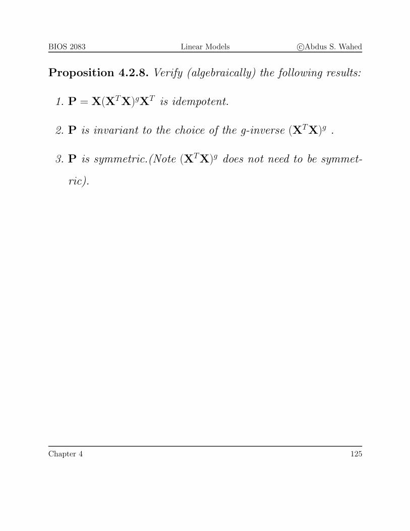
Proposition 4.2.8. Verify (algebraically) the following results:

1. P = X(XTX)gXT is idempotent.

2. P is invariant to the choice of the g-inverse (XTX)g .

3. P is symmetric.(Note (XTX)g does not need to be symmet-

ric).

Chapter 4 125


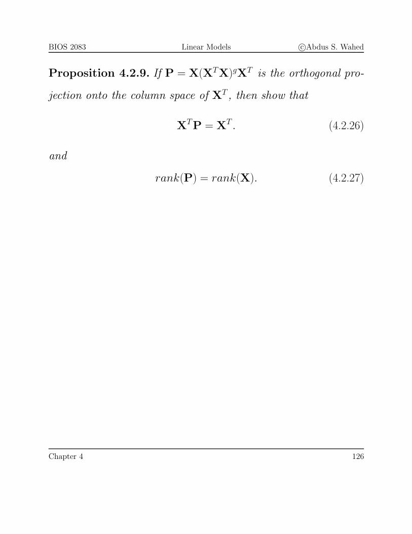
Proposition 4.2.9. If P = X(XTX)gXT is the orthogonal pro-

jection onto the column space of XT , then show that

XTP = XT . (4.2.26)

and

rank(P) = rank(X). (4.2.27)

Chapter 4 126


Residual vector

Definition 4.2.1. The vector e = Y − Y is known to be the

residual vector.

Notice,

e = Y − Y = (In − P)Y, (4.2.28)

and Y can be decomposed into two orthogonal components,

Y = Y + e, (4.2.29)

Y = PY belonging to the column space of X and e = (In − P)Y

belonging to N (XT ).

Example 4.2.10. Show that Y and e are uncorrelated when the

elements of Y are independent with equal variance.

Chapter 4 127


Proof. Let cov(Y) = σ2In. Then,

E(YeT ) = E(PYYT (In − P))

= PE(YYT )(In − P)

= P[σ2In + XββTXT

](In − P)

= σ2P(In − P)

= 0. (4.2.30)

Also, E [e] = 0. Together we get, cov(Y, e) = 0.

Chapter 4 128


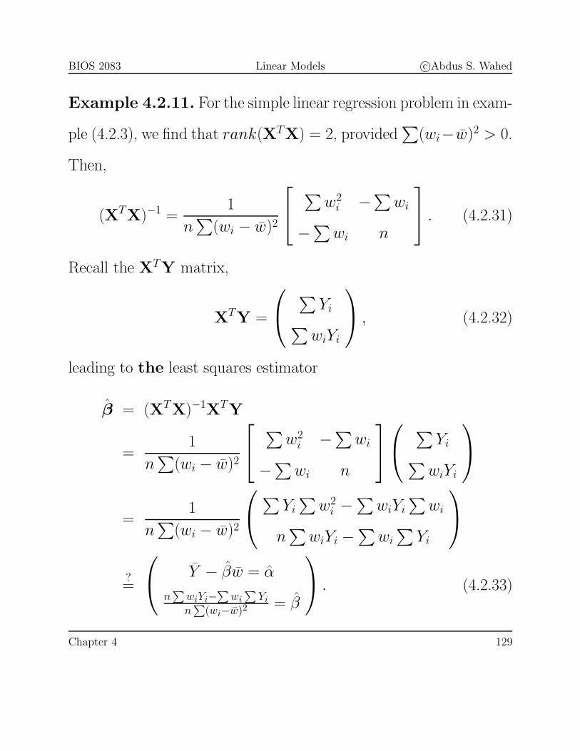
Example 4.2.11. For the simple linear regression problem in exam-

ple (4.2.3), we find that rank(XTX) = 2, provided∑

(wi−w)2 > 0.

Then,

(XTX)−1 =1

n∑

(wi − w)2

⎡⎣ ∑

w2i −∑wi

−∑wi n

⎤⎦ . (4.2.31)

Recall the XTY matrix,

XTY =

⎛⎝ ∑

Yi∑wiYi

⎞⎠ , (4.2.32)

leading to the least squares estimator

β = (XTX)−1XTY

=1

n∑

(wi − w)2

⎡⎣ ∑

w2i −∑wi

−∑wi n

⎤⎦⎛⎝ ∑

Yi∑wiYi

⎞⎠

=1

n∑

(wi − w)2

⎛⎝∑Yi

∑w2

i −∑

wiYi

∑wi

n∑

wiYi −∑

wi

∑Yi

⎞⎠

?=

⎛⎝ Y − βw = α

n∑

wiYi−∑

wi∑

Yi

n∑

(wi−w)2= β

⎞⎠ . (4.2.33)

Chapter 4 129


Example 4.2.12. For the one-way ANOVA model in Example

(4.2.4),

XTX =

⎡⎢⎢⎢⎢⎢⎢⎢⎣

n n1 n2 . . . na

n1 n1 0 . . . 0

... ... ... ... ...

na 0 0 . . . na

⎤⎥⎥⎥⎥⎥⎥⎥⎦

, (4.2.34)

A g-inverse is given by,

(XTX)g =

⎡⎢⎢⎢⎢⎢⎢⎢⎣

0 0 0 . . . 0

0 1/n1 0 . . . 0

... ... ... ... ...

0 0 0 . . . 1/na

⎤⎥⎥⎥⎥⎥⎥⎥⎦

, (4.2.35)

The projection, P is obtained as,

P = X(XTX)gXT = blockdiag

{1

niJni

, i = 1, 2, . . . , a.

}(4.2.36)

Chapter 4 130


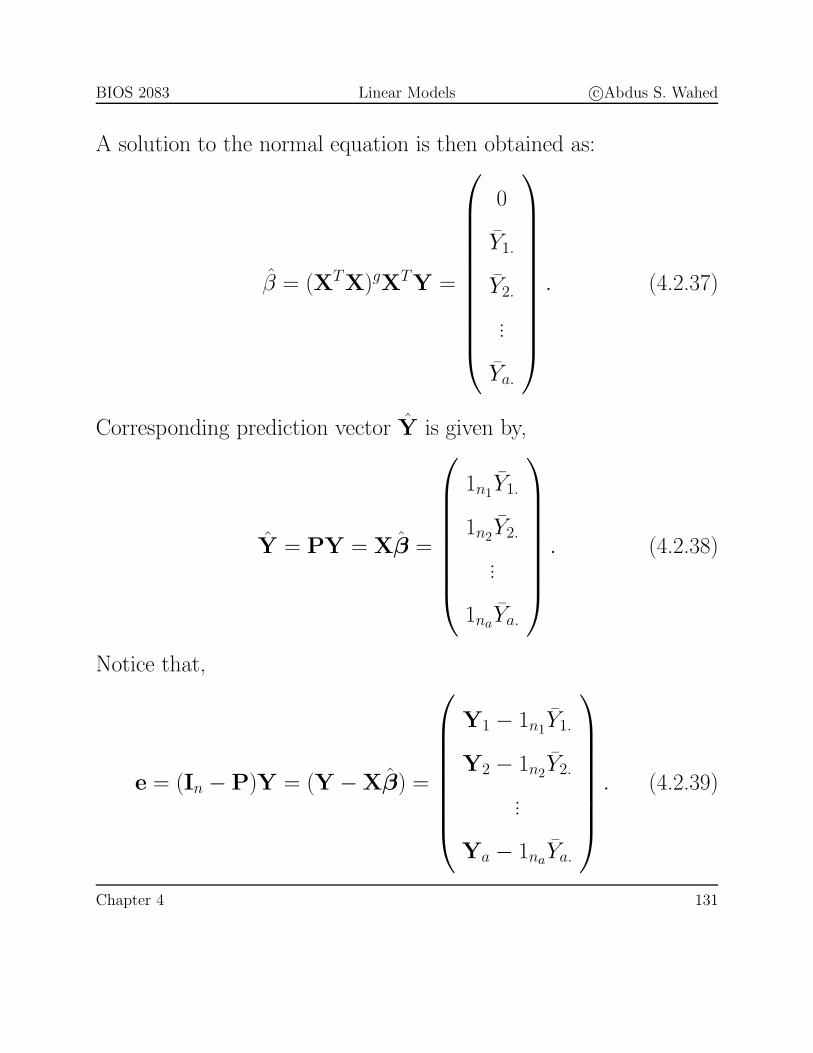
A solution to the normal equation is then obtained as:

β = (XTX)gXTY =

⎛⎜⎜⎜⎜⎜⎜⎜⎜⎜⎜⎝

0

Y1.

Y2.

...

Ya.

⎞⎟⎟⎟⎟⎟⎟⎟⎟⎟⎟⎠

. (4.2.37)

Corresponding prediction vector Y is given by,

Y = PY = Xβ =

⎛⎜⎜⎜⎜⎜⎜⎜⎝

1n1Y1.

1n2Y2.

...

1naYa.

⎞⎟⎟⎟⎟⎟⎟⎟⎠

. (4.2.38)

Notice that,

e = (In − P)Y = (Y − Xβ) =

⎛⎜⎜⎜⎜⎜⎜⎜⎝

Y1 − 1n1Y1.

Y2 − 1n2Y2.

...

Ya − 1naYa.

⎞⎟⎟⎟⎟⎟⎟⎟⎠

. (4.2.39)

Chapter 4 131


‖Y‖2 = YTY = n1Y21. + n2Y

22. + . . . + naY

2a.

=a∑

i=1

niY2i. . (4.2.40)

and

‖e‖2 = eTe = YT1 Y1 − n1Y

21. + YT

2 Y2 − n2Y22. + . . . + YT

a Ya − naY2a.

=a∑

i=1

{YT

i Yi − niY2i.

}=

a∑i=1

ni∑j=1

{Yij − Yi.

}2

=

a∑i=1

ni∑j=1

Y 2ij −

a∑i=1

niY2i.

= ‖Y‖2 − ‖Y‖2. (4.2.41)

“Residual SS” = Total SS -“Regression SS”. Or,

Total SS = “Regression SS” + “Residual SS”.

Chapter 4 132


Theorem 4.2.13. If β is a solution to the normal equations

(4.2.6), then,

‖Y‖2 = ‖Y‖2 + ‖e‖2, (4.2.42)

where, Y = Xβ and e = Y − Xβ.

Proof. Left as an exercise.

Definition 4.2.2. Regression SS, Residual SS. The quantity

‖Y‖2 is referred to as regression sum of squares or model sum of

squares, the portion of total sum of squares explained by the linear

model whereas the other part ‖e‖2 is the error sum of squares or

residual sum of squares (unexplained variation).

Coefficient of determination (R2)

To have a general definition, let the model Y = Xβ + ε contains an

intercept term, meaning the first column of X is 1n. Total sum of

Chapter 4 133


Table 4.1: Analysis of variance

Models with/without an intercept term

Source df SS

Regression (Model) r YTPY

Residual (Error) n − r YT (I −P)Y

Total n YTY

Models with an intercept term

Source df SS

Mean 1 YT 1n1TnY/n

Regression (corrected for mean) r − 1 YT (P− 1n1Tn/n)Y


Total n YTY

Models with an intercept term

Source df SS

Regression (corrected for mean) r − 1 YT (P− 1n1Tn/n)Y


Total (corrected) n − 1 YTY − YT1n1TnY/n

Chapter 4 134


squares corrected for the intercept term (or mean) is then written as

Total SS(corr.) = YTY − nY 2

= YT (In − 1

nJn)Y. (4.2.43)

Similarly, the regression SS is also corrected for the intercept term

and is expressed as

Regression SS(corr.) = YTPY − nY 2

= YT (P − 1

nJn)Y. (4.2.44)

This is the portion of total corrected sum of squares that is purely

explained by the design variables in the model. However, an equal-

ity similar to (4.4.42) applied to the corrected sums of squares still

follows, and the ratio

R2 =Reg. SS(Corr.)

Total SS(Corr.)=

YT (P − 1nJn)Y

YT (In − 1nJn)Y

(4.2.45)

explains the proportion of total variation explained by the

model. This ratio is known as the coefficient of determination and is

denoted by R2.

Chapter 4 135


Two important results:

Lemma 4.2.14. Ip − (XTX)gXTX is a projection onto N (X).

Proof. Use lemma 2.7.10.

Lemma 4.2.15. XTX(XTX)g is a projection onto C(XT ).

Proof. Use lemma 2.7.11.

Importance:

Sometimes it is easy to obtain a basis for the null space of X

or column space of XT by careful examination of the relationship

between the columns of X. However, in some cases it is not as

straightforward. In such cases, independent non-zero columns from

the projection matrix Ip − (XTX)gXTX can be used as a basis for

the null space of X. Similarly, independent non-zero columns from

the projection matrix XTX(XTX)g can be used as a basis for the

column space of XT .

Chapter 4 136


Example 4.2.16. Example 4.2.12 continued.

XTX(XTX)g =

⎡⎢⎢⎢⎢⎢⎢⎢⎢⎢⎢⎣

0 1 1 . . . 1

0 1 0 . . . 0

0 0 1 . . . 0

... ... ... ... ...

0 0 0 . . . 1

⎤⎥⎥⎥⎥⎥⎥⎥⎥⎥⎥⎦

. (4.2.46)

Therefore a basis for the column space of XT is given by the last n

columns of the above matrix. Similarly,

Ia+1 − (XTX)gXTX =

⎡⎢⎢⎢⎢⎢⎢⎢⎢⎢⎢⎣

1 0 0 . . . 0

−1 0 0 . . . 0

−1 0 0 . . . 0

... ... ... ... ...

−1 0 0 . . . 0

⎤⎥⎥⎥⎥⎥⎥⎥⎥⎥⎥⎦

. (4.2.47)

Therefore, the only basis vector in the null space of X is (1,−1Ta )T .

Chapter 4 137


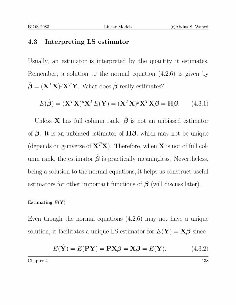
4.3 Interpreting LS estimator

Usually, an estimator is interpreted by the quantity it estimates.

Remember, a solution to the normal equation (4.2.6) is given by

β = (XTX)gXTY. What does β really estimates?

E(β) = (XTX)gXTE(Y) = (XTX)gXTXβ = Hβ. (4.3.1)

Unless X has full column rank, β is not an unbiased estimator

of β. It is an unbiased estimator of Hβ, which may not be unique

(depends on g-inverse of XTX). Therefore, when X is not of full col-

umn rank, the estimator β is practically meaningless. Nevertheless,

being a solution to the normal equations, it helps us construct useful

estimators for other important functions of β (will discuss later).

Estimating E(Y)

Even though the normal equations (4.2.6) may not have a unique

solution, it facilitates a unique LS estimator for E(Y) = Xβ since

E(Y) = E(PY) = PXβ = Xβ = E(Y). (4.3.2)

Chapter 4 138


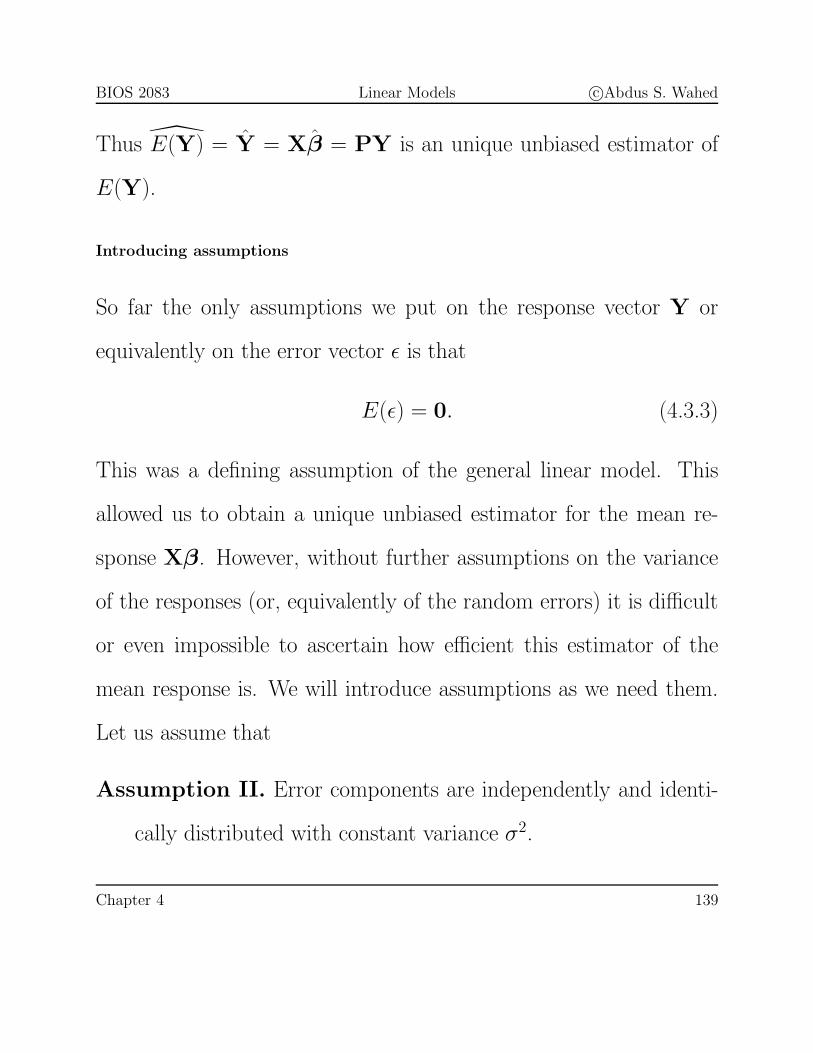
Thus E(Y) = Y = Xβ = PY is an unique unbiased estimator of

E(Y).

Introducing assumptions

So far the only assumptions we put on the response vector Y or

equivalently on the error vector ε is that

E(ε) = 0. (4.3.3)

This was a defining assumption of the general linear model. This

allowed us to obtain a unique unbiased estimator for the mean re-

sponse Xβ. However, without further assumptions on the variance

of the responses (or, equivalently of the random errors) it is difficult

or even impossible to ascertain how efficient this estimator of the

mean response is. We will introduce assumptions as we need them.

Let us assume that

Assumption II. Error components are independently and identi-

cally distributed with constant variance σ2.

Chapter 4 139


Variance-covariance matrix for LS estimator

Under assumption II, cov(Y) = σ2In. Variance-covariance matrix

cov(β) of a LS estimator β = (XTX)gXTY is given by

cov(β) = cov((XTX)gXTY)

= (XTX)gXTcov(Y)[(XTX)gXT

]T= (XTX)gXTX

[(XTX)g

]Tσ2 (4.3.4)

For full rank cases (4.3.4) reduces to the familiar form cov(β) =

(XTX)−1σ2.

Variance-covariance matrix for Y

Example 4.3.1. Show that

1. cov(Y) = Pσ2.

2. cov(e) = (I − P)σ2.

Chapter 4 140


Estimating the error variance

Note that, using Theorem 3.4.7,

E(Residual SS) = E[YT (I − P)Y

]= trace

{(I − P)σ2In

}+ (Xβ)T (I − P)Xβ

= σ2trace {(I− P)} + βTXT (I − P)Xβ

= σ2(n − r), (4.3.5)

where r = rank(X). Therefore, an unbiased estimator of the error

variance σ2 is given by

σ2 =Residual SS

n − r=

Residual MS

n − r=

YT (I− P)Y

n − r. (4.3.6)

4.4 Estimability

Unless X is of full column rank, solution to the normal equations

(4.2.6) is not unique. Therefore, in such cases, a solution to the

normal equation does not estimate any useful population quantity.

More specifically, we have shown that E(β) = Hβ, where H =

Chapter 4 141


(XTX)gXTX. Consider the following XTX matrix

XTX =

⎡⎢⎢⎢⎢⎣

6 3 3

3 3 0

3 0 3

⎤⎥⎥⎥⎥⎦ (4.4.1)

from a one-way ANOVA experiment with two treatments each repli-

cated 3 times. Let us consider two g-inverses

G1 =

⎡⎢⎢⎢⎢⎣

0 0 0

0 1/3 0

0 0 1/3

⎤⎥⎥⎥⎥⎦ (4.4.2)

and

G2 =

⎡⎢⎢⎢⎢⎣

1/3 −1/3 0

−1/3 2/3 0

0 0 0

⎤⎥⎥⎥⎥⎦ (4.4.3)

with

H1 = G1XTX =

⎡⎢⎢⎢⎢⎣

0 0 0

1 1 0

1 0 1

⎤⎥⎥⎥⎥⎦ (4.4.4)

Chapter 4 142


and

H2 = G2XTX =

⎡⎢⎢⎢⎢⎣

1 0 1

0 1 −1

0 0 0

⎤⎥⎥⎥⎥⎦ (4.4.5)

respectively. Now, if β = (μ, α1, α2)T , then,

H1β =

⎛⎜⎜⎜⎜⎝

0

μ + α1

μ + α2

⎞⎟⎟⎟⎟⎠ (4.4.6)

whereas

H2β =

⎛⎜⎜⎜⎜⎝

μ + α1

α1 − α2

0

⎞⎟⎟⎟⎟⎠ . (4.4.7)

Thus two solutions to the same normal equations set estimate two

different quantities. However, in practice, one would like to construct

estimators that estimate the same population quantity, no matter

what solution to the normal equation is used to derive that estimator.

One important goal in one-way ANOVA is to estimate the difference

Chapter 4 143


between two treatment effects, namely, δ = α1 − α2 = (0, 1,−1)β.

Two different solutions based on the two g-inverses G1 and G2 are

given by β1 = (0, Y1., Y2.)T and β2 = (Y2., Y1. − Y2., 0)T . If we

construct our estimator for δ based on the solution β1, we obtain

δ1 = (0, 1,−1)β1 = Y1. − Y2., (4.4.8)

exactly the quantity you would expect. Now let us see if the same

happens with the other solution β2. For this solution,

δ2 = (0, 1,−1)β2 = Y1. − Y2., (4.4.9)

same as δ1. Now we will show that no matter what solution you pick

for the normal equation, δ will always be the same. To see it, let us

write δ as

δ = (0, 1,−1)(XTX)gXTY

= PδY, (4.4.10)

where Pδ = (0, 1,−1)(XTX)gXT . If we can show that Pδ does not

depend on the choice of g-inverse (XTX)g, then we are through. Let

Chapter 4 144


us first look at the XT -matrix for this simpler version of one-way

ANOVA problem:

XT =

⎡⎢⎢⎢⎢⎣

1 1 1 1 1 1

1 1 1 0 0 0

0 0 0 1 1 1

⎤⎥⎥⎥⎥⎦ . (4.4.11)

Notice that, (0, 1,−1)T belongs to C(XT ), e.g.

⎛⎜⎜⎜⎜⎝

0

1

−1

⎞⎟⎟⎟⎟⎠ =

⎡⎢⎢⎢⎢⎣

1 1 1 1 1 1

1 1 1 0 0 0

0 0 0 1 1 1

⎤⎥⎥⎥⎥⎦

⎛⎜⎜⎜⎜⎜⎜⎜⎜⎜⎜⎜⎜⎜⎝

1

0

0

−1

0

0

⎞⎟⎟⎟⎟⎟⎟⎟⎟⎟⎟⎟⎟⎟⎠

. (4.4.12)

But we know that there exists a unique c ∈ C(X) such that

(0, 1,−1)T = XTc. Now,

Pδ = (0, 1,−1)(XTX)gXT = cTX(XTX)gXT = cTP. (4.4.13)

Since c is unique, and P does not depend on the choice of (XTX)g,

Chapter 4 145


from the above equation we see that Pδ, and hence δ = PδY is

unique to the choice of a g-inverse.

Summary

• Not all linear functions of β may be estimated uniquely based

on the LS method.

• Linear functions λTβ of β, where λ is a linear combination of

the columns of XT allow unique estimators based on the LS

estimator.

Estimable functions

Definition 4.4.1. θ(Y) is an unbiased estimator of θ if and only

if E[θ(Y)

]= θ, for all θ.

Definition 4.4.2. θ(Y) is a linear estimator of θ if and only if

θ(Y) = aTY + b, for some constant (vector) b and vector (matrix)

a.

Chapter 4 146


Definition 4.4.3. A linear function θ = λTβ is linearly estimable

if and only if there exists a linear function cTY such that E(cTY) =

λTβ = θ, for all β.

We will drop “linearly” from “linearly estimable” for simplicity.

That means “estimable” will always refer to linearly estimable unless

mentioned specifically.

Example 4.4.1.

1. Components of the mean vector Xβ are estimable.

2. Components of the vector XTXβ are estimable.

Proposition 4.4.2. Linear combinations of estimable functions

are estimable.

Proof. Follows from the definition 4.4.3.

Chapter 4 147


Proposition 4.4.3. A linear function θ = λTβ is estimable if

and only if λ ∈ C(XT ).

Proof. Suppose θ = λTβ is estimable. Then, by definition, there

exists a vector c such that

E(cTY) = λTβ, for all β

=⇒ cTXβ = λTβ, for all β

=⇒ cTX = λT ,

=⇒ λ = XTc

=⇒ λ ∈ C(XT ). (4.4.14)

Now, suppose λ ∈ C(XT ). This implies that λ = XTc for some c.

Then, for all β,

λTβ = cTXβ = cTE(Y) = E(cTY). (4.4.15)

Chapter 4 148


Proposition 4.4.4. If θ = λTβ is estimable then there exists a

unique c∗ ∈ C(X) such that λ = XTc∗.

Proof. Proposition 4.4.3 indicates that there exists a c such that

λ = XTc. But any vector c can be written as a direct sum of two

unique components belonging to two orthogonal complements. Thus,

we can find c∗ ∈ C(X) and c∗∗ ∈ N (XT ) such that

c = c∗ + c∗∗. (4.4.16)

Now

λ = XTc = XTc∗ + XTc∗∗ = XTc∗. (4.4.17)

Hence, the proof.

Proposition 4.4.5. Collection of all possible estimable func-

tions constitutes a vector space of dimension r = rank(X).

Proof. Hint: (i) Show that linear combinations of estimable func-

tions are also estimable, and (ii) Use proposition 4.4.3.

Chapter 4 149


Methods to determine estimability

Method 1. λTβ is estimable if and only if it can be expressed as a linear

combinations of the rows of Xβ.

Method 2. λTβ is estimable if and only if λTe = 0 for all bassis vectors e

of the null space of X.

Method 3. λTβ is estimable if and only if λ is a linear combination of the

basis vectors of C(XT ).

Example 4.4.6. Multiple linear regression (Example 1.1.5

continued..) In the case of multiple regression with p independent

variables (which may include the intercept term) and n observations

(n > p) , columns of X are all independent. Therefore, N (X) = {0}.By method 2, all linear functions of β are estimable. In particular,

1. Individual coefficients βj are estimable.

2. Differences between two coefficients are estimable.

Chapter 4 150



1. Treatment-specific means μ + αi, i = 1, 2, . . . , a are estimable

(using Method 1).

2. Difference between two treatment effects (αi − αi′) is estimable.

(Follows from the above, or can be inferred by Method 2).

3. In general, any linear combination λTβ = λ0μ +∑a

i=1 λiαi is

estimable if and only if λ0 =∑a

i=1 λi. (Use Method 2).

Chapter 4 151


Example 4.4.8. Two-way nested design. Suppose ni patients

are randomized to the ith level of treatment A, i = 1, 2, . . . , a and

within the ith treatment group a second randomization is done to bi

levels of treatment B which are unique to each level of treatment A.

The linear model for this problem can be written as

Yijk = μ + αi + βij + εijk,

i = 1, 2, . . . , a; j = 1, 2, . . . , bi; k = 1, 2, . . . , nij.(4.4.18)

Then the X−matrix for this problem is given by

X =

⎡⎢⎢⎢⎢⎢⎢⎢⎢⎢⎢⎢⎢⎢⎢⎢⎢⎢⎢⎢⎣

1 1 0 1 0 0 0

1 1 0 1 0 0 0

1 1 0 0 1 0 0

1 1 0 0 1 0 0

1 0 1 0 0 1 0

1 0 1 0 0 1 0

1 0 1 0 0 0 1

1 1 1 0 0 0 1

⎤⎥⎥⎥⎥⎥⎥⎥⎥⎥⎥⎥⎥⎥⎥⎥⎥⎥⎥⎥⎦

, (4.4.19)

Chapter 4 152


where we have simplified the problem by taking a = 2, b1 = b2 = 2,

and n11 = n12 = n21 = n22 = 2. Clearly rank(X) = 4. Dimension

of the null space of X is 7 - 4 = 3. A set of basis vectors for the null

space of X can be written as:

e1 =

⎛⎜⎜⎜⎜⎜⎜⎜⎜⎜⎜⎜⎜⎜⎜⎜⎜⎝

1

0

0

−1

−1

−1

−1

⎞⎟⎟⎟⎟⎟⎟⎟⎟⎟⎟⎟⎟⎟⎟⎟⎟⎠

, e2 =

⎛⎜⎜⎜⎜⎜⎜⎜⎜⎜⎜⎜⎜⎜⎜⎜⎜⎝

0

1

0

−1

−1

0

0

⎞⎟⎟⎟⎟⎟⎟⎟⎟⎟⎟⎟⎟⎟⎟⎟⎟⎠

, e3 =

⎛⎜⎜⎜⎜⎜⎜⎜⎜⎜⎜⎜⎜⎜⎜⎜⎜⎝

0

0

1

0

0

−1

−1

⎞⎟⎟⎟⎟⎟⎟⎟⎟⎟⎟⎟⎟⎟⎟⎟⎟⎠

(4.4.20)

Thus, using Method 2, λTβ is estimable if

λTej = 0, j = 1, 2, 3. (4.4.21)

Specifically, if λ = (λ0, λ1, λ2, λ11, λ12, λ21, λ22)T , then λTβ is es-

Chapter 4 153


timable if the following three conditions are satisfied:

(1) λ0 =

2∑i=1

2∑j=1

λij,

(2) λ1 =

2∑j=1

λ1j,

(3) λ2 =

2∑j=1

λ2j. (4.4.22)

Let us consider some special cases:

1. Is α1 estimable?

2. Is μ + α1 estimable?

3. Is α1 − α2 estimable?

4. Is α1 − α2 + (β11 + β12)/2 − (β21 + β22)/2 estimable?

Chapter 4 154


Definition 4.4.4. Least squares estimator of an estimable

function λTβ is given by λT β, where β is a solution to the normal

equations (4.2.6).

Properties of least squares estimator

Proposition 4.4.9. Uniqueness. Least squares estimator (of

an estimable function) is invariant to the choice of a solution to

the normal equations.

Proof. Let us consider the class of solutions from the normal equa-

tions

β = (XTX)gXTY.

Least squares estimator of a an estimable function λTβ is then given

by

λT β = λT (XTX)TXTY. (4.4.23)

From proposition 4.4.4, since λTβ is estimable, there exists a unique

c ∈ C(X) such that

λ = XTc. (4.4.24)

Chapter 4 155


Therefore, Equation (4.4.23) combined with (4.4.24) leads to

λT β = cTX(XTX)gXTY = cTPY. (4.4.25)

Since both c and P are unique (does not depend on the choice of

g-inverse), the result follows.

Proposition 4.4.10. Linearity and Unbiasedness. LS esti-

mator is linear and unbiased.

Proof. Left as an exercise.

Proposition 4.4.11. Variance. Under Assumption II,

V ar(λT β) = σ2λT (XTX)gλ. (4.4.26)

Proof.

V ar(λT β) = V ar[λT (XTX)gXTY

]= λT (XTX)gXTcov(Y)

{λT (XTX)gXT

}T

= σ2λT (XTX)gXTX{(XTX)g

}Tλ

?= σ2λT (XTX)gλ. (4.4.27)

Chapter 4 156


Proposition 4.4.12. Characterization. If an estimator λT β

of a linear function λTβ is invariant to the choice of the solutions

β to the normal equations, then λTβ is estimable.

Proof. For a given g-inverse G of XTX, consider the general form

of the solutions to the normal equations:

β = GXTY + (I − GXTX)c (4.4.28)

for any vector c ∈ Rp. Then,

λT β = λT{GXTY + (I − GXTX)c

}= λTGXTY + λT (I− GXTX)c. (4.4.29)

Since G is given, in order for the above to be equal for all c, we must

have

λT (I − GXTX) = 0. (4.4.30)

Or, equivalently,

λT = λTGXTX. (4.4.31)

This last equation implies that λ ∈ C(XT ). This completes the

proof.

Chapter 4 157


Theorem 4.4.13. Gauss-Markov Theorem. Under Assump-

tions I and II, if λTβ is estimable, then the least squares es-

timator λT β is the unique minimum variance linear unbiased

estimator.

In the econometric literature, minimum variance is referred to as

best and along with the linearity and unbiasedness the least squares

estimator becomes best linear unbiased estimator (BLUE).

Proof. Uniqueness follows from the proposition 4.4.9. Linearity and

unbiasedness follows from the proposition 4.4.10. The only thing

remains to be shown is that no other linear unbiased estimator of

λTβ can have smaller variance than λT β.

Since λTβ is estimable, there exists a c such that λ = XTc. Let

a + dTY be any other linear unbiased estimator of λTβ. Then, we

Chapter 4 158


must have a = 0 and λT = dTX. Then,

XTd = XTc

=⇒ XT (c− d) = 0

=⇒ (c− d) ∈ N (XT )

=⇒ P(c − d) = 0

=⇒ Pc = Pd. (4.4.32)

Now, by proposition 4.4.11,

var(λT β) = σ2cTX(XTX)gXTc = σ2cTPc. (4.4.33)

and

var(dTY) = σ2dTd. (4.4.34)

Chapter 4 159


Thus,

var(dTY) − var(λT β) = σ2{dTd− cTPc

}= σ2

{dTd− cTP2c

}= σ2

{dTd− dTP2d

}= σ2dT (I − P)d (4.4.35)

≥ 0.

Therefore the LS estimator has the minimum variance among all lin-

ear unbiased estimators. Equation (4.4.35) shows that var(dTY) =

var(λT β) if and only if (I−P)d = 0, or equivalently, d = Pd = Pc,

leading to dTY = cTPY = cTX(XTX)gXTY = λT β.

Chapter 4 160



XTX =

⎡⎢⎢⎢⎢⎢⎢⎢⎢⎢⎢⎢⎢⎢⎢⎢⎢⎣

8 4 4 2 2 2 2

4 4 0 2 2 0 0

4 0 4 0 0 2 2

2 2 0 2 0 0 0

2 2 0 0 2 0 0

2 0 2 0 0 2 0

2 0 2 0 0 0 2

⎤⎥⎥⎥⎥⎥⎥⎥⎥⎥⎥⎥⎥⎥⎥⎥⎥⎦

, (4.4.36)

a g-inverse of which is given by,

(XTX)g =

⎡⎢⎢⎢⎢⎢⎢⎢⎢⎢⎢⎢⎢⎢⎢⎢⎢⎣

0 0 0 0 0 0 0

0 0 0 0 0 0 0

0 0 0 0 0 0 0

0 0 0 1/2 0 0 0

0 0 0 0 1/2 0 0

0 0 0 0 0 1/2 0

0 0 0 0 0 0 1/2

⎤⎥⎥⎥⎥⎥⎥⎥⎥⎥⎥⎥⎥⎥⎥⎥⎥⎦

. (4.4.37)

Chapter 4 161


XTY =

⎡⎢⎢⎢⎢⎢⎢⎢⎢⎢⎢⎢⎢⎢⎢⎢⎢⎢⎢⎢⎣

1 1 0 1 0 0 0

1 1 0 1 0 0 0

1 1 0 0 1 0 0

1 1 0 0 1 0 0

1 0 1 0 0 1 0

1 0 1 0 0 1 0

1 0 1 0 0 0 1

1 1 1 0 0 0 1

⎤⎥⎥⎥⎥⎥⎥⎥⎥⎥⎥⎥⎥⎥⎥⎥⎥⎥⎥⎥⎦

T ⎛⎜⎜⎜⎜⎜⎜⎜⎜⎜⎜⎜⎜⎜⎜⎜⎜⎜⎜⎜⎝

Y111

Y112

Y121

Y122

Y211

Y212

Y221

Y222

⎞⎟⎟⎟⎟⎟⎟⎟⎟⎟⎟⎟⎟⎟⎟⎟⎟⎟⎟⎟⎠

=

⎛⎜⎜⎜⎜⎜⎜⎜⎜⎜⎜⎜⎜⎜⎜⎜⎜⎝

Y...

Y1..

Y2..

Y11.

Y12.

Y21.

Y22.

⎞⎟⎟⎟⎟⎟⎟⎟⎟⎟⎟⎟⎟⎟⎟⎟⎟⎠

(4.4.38)

Thus, a solution to the normal equations is given by

⎛⎜⎜⎜⎜⎜⎜⎜⎜⎜⎜⎜⎜⎜⎜⎜⎜⎝

μ

α1

α2

β11

β12

β21

β22

⎞⎟⎟⎟⎟⎟⎟⎟⎟⎟⎟⎟⎟⎟⎟⎟⎟⎠

= (XTX)gXTY =

⎛⎜⎜⎜⎜⎜⎜⎜⎜⎜⎜⎜⎜⎜⎜⎜⎜⎝

0

0

0

Y11.

Y12.

Y21.

Y22.

⎞⎟⎟⎟⎟⎟⎟⎟⎟⎟⎟⎟⎟⎟⎟⎟⎟⎠

. (4.4.39)

Therefore the linear MVUE (or BLUE) of the estimable function

α1 −α2 + (β11 + β12)/2− (β21 + β22)/2 is given by (Y11. + Y12.)/2−(Y21. + Y22.)/2.

Chapter 4 162


4.4.1 A comment on estimability and Missing data

The concept of estimability is very important in drawing statistical

inference from a linear model. What effects can be estimated from

an experiment totally depends on how the experiment was designed.

For instance, in a two-way nested model, difference between two

main effects is not estimable, whereas difference between two nested

effects within the same main effect is. In an over-parameterized one-

way ANOVA model (One-way ANOVA with an intercept term), the

treatment effects are not estimable while the difference between any

two pair of treatments is estimated by the difference in corresponding

cell means.

When observations in some cells are missing, the problem of es-

timability becomes more acute. We illustrate the concept by using an

example. Consider the two-way nested design considered in Example

4.4.8. Suppose after planning the experiment, the observation cor-

responding to the last two rows of X matrix could not be observed.

Chapter 4 163


Thus the observed design matrix is given by

XM =

⎡⎢⎢⎢⎢⎢⎢⎢⎢⎢⎢⎢⎢⎢⎣

1 1 0 1 0 0 0

1 1 0 1 0 0 0

1 1 0 0 1 0 0

1 1 0 0 1 0 0

1 0 1 0 0 1 0

1 0 1 0 0 1 0

⎤⎥⎥⎥⎥⎥⎥⎥⎥⎥⎥⎥⎥⎥⎦

. (4.4.40)

How does this effect the estimability of certain functions? Note that

rank(XM) = 3. A basis for the null space of XT is given by⎧⎪⎪⎪⎪⎪⎪⎪⎪⎪⎪⎪⎪⎪⎪⎪⎪⎨⎪⎪⎪⎪⎪⎪⎪⎪⎪⎪⎪⎪⎪⎪⎪⎪⎩

e1 =

⎛⎜⎜⎜⎜⎜⎜⎜⎜⎜⎜⎜⎜⎜⎜⎜⎜⎝

1

0

0

−1

−1

−1

1

⎞⎟⎟⎟⎟⎟⎟⎟⎟⎟⎟⎟⎟⎟⎟⎟⎟⎠

, e2 =

⎛⎜⎜⎜⎜⎜⎜⎜⎜⎜⎜⎜⎜⎜⎜⎜⎜⎝

0

1

0

−1

−1

0

1

⎞⎟⎟⎟⎟⎟⎟⎟⎟⎟⎟⎟⎟⎟⎟⎟⎟⎠

, e3 =

⎛⎜⎜⎜⎜⎜⎜⎜⎜⎜⎜⎜⎜⎜⎜⎜⎜⎝

0

0

1

0

0

−1

1

⎞⎟⎟⎟⎟⎟⎟⎟⎟⎟⎟⎟⎟⎟⎟⎟⎟⎠

, e4 =

⎛⎜⎜⎜⎜⎜⎜⎜⎜⎜⎜⎜⎜⎜⎜⎜⎜⎝

0

0

0

0

0

0

1

⎞⎟⎟⎟⎟⎟⎟⎟⎟⎟⎟⎟⎟⎟⎟⎟⎟⎠

⎫⎪⎪⎪⎪⎪⎪⎪⎪⎪⎪⎪⎪⎪⎪⎪⎪⎬⎪⎪⎪⎪⎪⎪⎪⎪⎪⎪⎪⎪⎪⎪⎪⎪⎭

. (4.4.41)

1. Is α1 estimable?

α1 = (0, 1, 0, 0, 0, 0, 0)β = λT1 β.

λT1 e1 = 0 �= λT

1 e2 → Not estimable.

Chapter 4 164


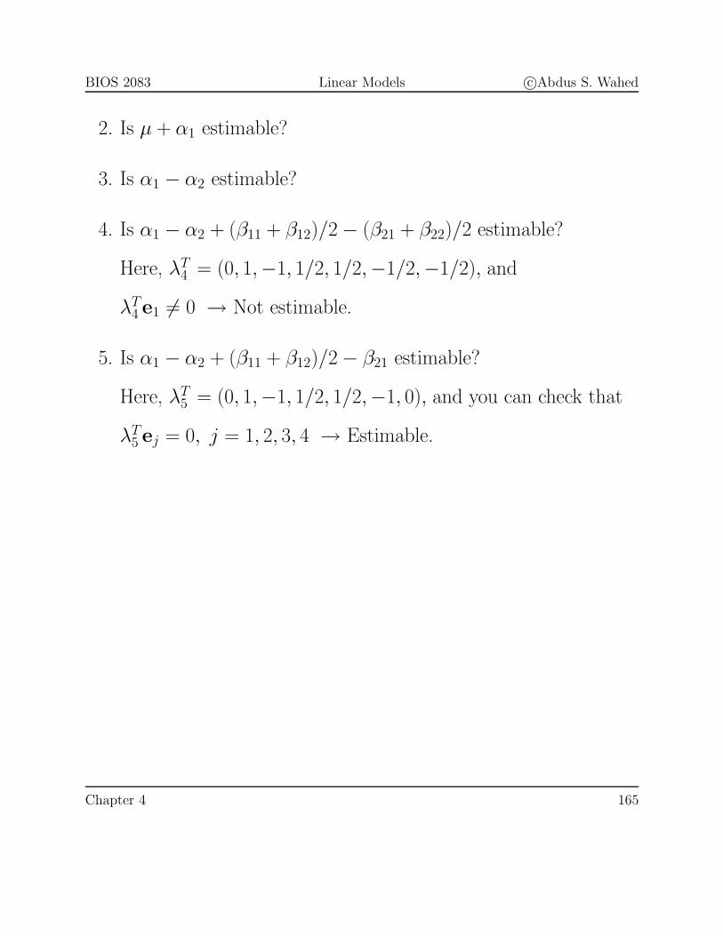
2. Is μ + α1 estimable?

3. Is α1 − α2 estimable?

4. Is α1 − α2 + (β11 + β12)/2 − (β21 + β22)/2 estimable?

Here, λT4 = (0, 1,−1, 1/2, 1/2,−1/2,−1/2), and

λT4 e1 �= 0 → Not estimable.

5. Is α1 − α2 + (β11 + β12)/2 − β21 estimable?

Here, λT5 = (0, 1,−1, 1/2, 1/2,−1, 0), and you can check that

λT5 ej = 0, j = 1, 2, 3, 4 → Estimable.

Chapter 4 165


4.5 Least squares estimation under linear constraints

Often it is desirable to estimate the parameters from a linear model

under certain linear constraints. Two possible scenarios where such

constrained minimization of the error sum of squares (‖Y − Xβ‖2)

becomes handy are as follows.

1. Converting a non-full rank model to a full rank model.

A model of non-full rank can be transformed into a full rank

model by imposing a linear constraint on the model. Let us

take a simple example of a balanced one-way ANOVA with two

treatments. The over-parameterized version of this model can

be written as

Yij = μ + αi + εij, i = 1, 2; j = 1, 2, . . . , n. (4.5.1)

We know from our discussion that αi is not estimable in this

model. We also know that the X-matrix is not of full rank,

Chapter 4 166


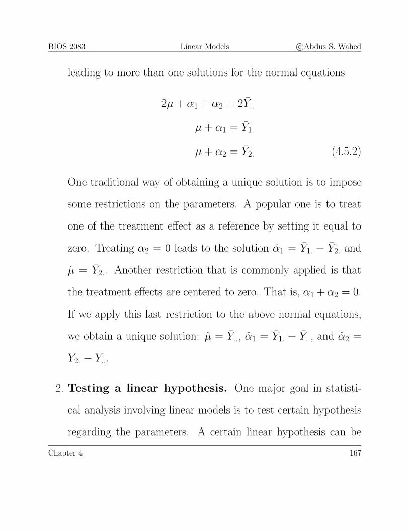
leading to more than one solutions for the normal equations

2μ + α1 + α2 = 2Y..

μ + α1 = Y1.

μ + α2 = Y2. (4.5.2)

One traditional way of obtaining a unique solution is to impose

some restrictions on the parameters. A popular one is to treat

one of the treatment effect as a reference by setting it equal to

zero. Treating α2 = 0 leads to the solution α1 = Y1. − Y2. and

μ = Y2.. Another restriction that is commonly applied is that

the treatment effects are centered to zero. That is, α1 + α2 = 0.

If we apply this last restriction to the above normal equations,

we obtain a unique solution: μ = Y.., α1 = Y1. − Y.., and α2 =

Y2. − Y...

2. Testing a linear hypothesis. One major goal in statisti-

cal analysis involving linear models is to test certain hypothesis

regarding the parameters. A certain linear hypothesis can be

Chapter 4 167


tested by comparing the residual sum of squares from the model

under the null hypothesis to the same from unrestricted model

(no hypothesis). Details will follow in Chapter 6.

4.5.1 Restricted Least Squares

Suppose the linear model is of the form

Y = Xβ + ε, (4.5.3)

where a set of linear restrictions

ATβ = b (4.5.4)

has been imposed on the parameters for given matrices A and b.

We want to minimize the residual sum of squares

‖Y − Xβ‖2 = (Y − Xβ)T (Y − Xβ) (4.5.5)

for β to obtain the LS estimators under the constraints (4.5.4).The

problem can easily be written as a Lagrangian optimization problem

by constructing the objective function

E = (Y − Xβ)T (Y − Xβ) + 2λT (ATβ − b), (4.5.6)

Chapter 4 168


which needs to be minimized unconditionally with respect to β and

λ. Taking the derivatives of (4.5.6) with respect to β and λ and

setting them equal to zero, we obtain,

XTXβ + Aλ = XTY (4.5.7)

ATβ = b. (4.5.8)

The above equations will be referred to as restricted normal equations

(RNE). We will consider two different scenarios.

CASE I. ATβ is estimable.

A set of q linear constraints ATβ is estimable if and only if each

constraint is estimable. If we write A as (a1 a2 . . . aq) and b =

(b1, b2, . . . , bq), then ATβ is estimable iff each component aTi β is

estimable. Although, the q constraints need not be independently

estimable, but we assume that they are so that is rank(A) = q.

If they are not, one can easily reduce them into a set of linearly

independent constraints.

Now, if (βr, λr) is a solution to the restricted normal equations,

Chapter 4 169


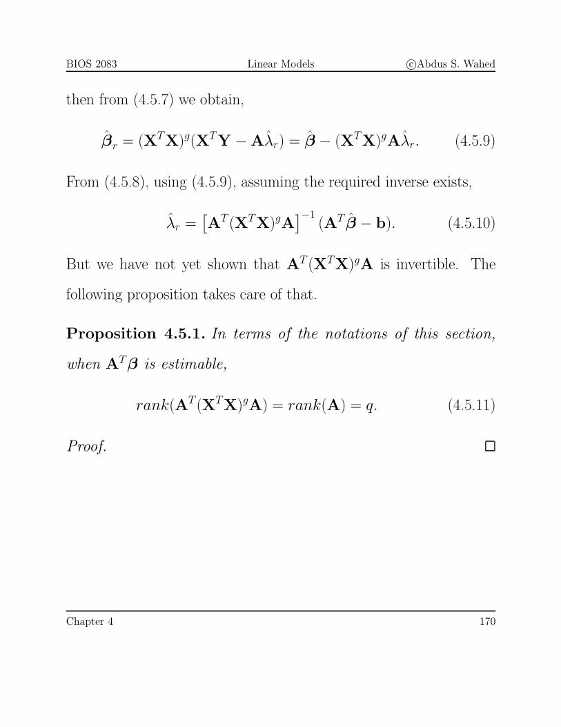
then from (4.5.7) we obtain,

βr = (XTX)g(XTY − Aλr) = β − (XTX)gAλr. (4.5.9)

From (4.5.8), using (4.5.9), assuming the required inverse exists,

λr =[AT (XTX)gA

]−1(AT β − b). (4.5.10)

But we have not yet shown that AT (XTX)gA is invertible. The

following proposition takes care of that.

Proposition 4.5.1. In terms of the notations of this section,

when ATβ is estimable,

rank(AT (XTX)gA) = rank(A) = q. (4.5.11)

Proof.

Chapter 4 170


Using (4.5.9) and (4.5.10), it is possible to express the restricted

least square estimator βr in terms of an unrestricted LS estimator

β:

βr = β − (XTX)gA[AT (XTX)gA

]−1(AT β − b). (4.5.12)

Example 4.5.2. Take the simple example of one-way balanced

ANOVA from the beginning of this section. Consider the restric-

tion α1 − α2 = 0, which can be written as ATβ = 0, where

A =

⎛⎜⎜⎜⎜⎝

0

1

−1

⎞⎟⎟⎟⎟⎠ (4.5.13)

A g-inverse of the XTX-matrix is given by⎛⎜⎜⎜⎝

0 0 0

0 1/n 0

0 0 1/n

⎞⎟⎟⎟⎠ (4.5.14)

with corresponding unrestricted solution,

β =

⎛⎜⎜⎜⎝

0

Y1.

Y2.

⎞⎟⎟⎟⎠ . (4.5.15)

Chapter 4 171


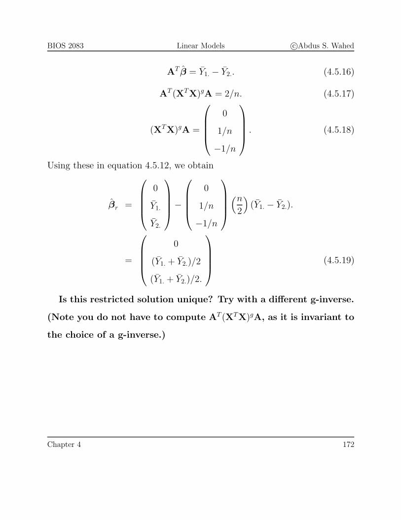
AT β = Y1. − Y2.. (4.5.16)

AT (XTX)gA = 2/n. (4.5.17)

(XTX)gA =

⎛⎜⎜⎜⎝

0

1/n

−1/n

⎞⎟⎟⎟⎠ . (4.5.18)

Using these in equation 4.5.12, we obtain

βr =

⎛⎜⎜⎜⎝

0

Y1.

Y2.

⎞⎟⎟⎟⎠−

⎛⎜⎜⎜⎝

0

1/n

−1/n

⎞⎟⎟⎟⎠(n

2

)(Y1. − Y2.).

=

⎛⎜⎜⎜⎝

0

(Y1. + Y2.)/2

(Y1. + Y2.)/2.

⎞⎟⎟⎟⎠ (4.5.19)

Is this restricted solution unique? Try with a different g-inverse.

(Note you do not have to compute AT (XTX)gA, as it is invariant to

the choice of a g-inverse.)

Chapter 4 172


Properties of restricted LS estimator

Proposition 4.5.3. 1. E[βr

]= (XTX)gXTXβ = Hβ = E

[β].

2. cov(βr

)= σ2

{(XTX)gD

[(XTX)g

]T}, where D = I−A

[AT (XTX)gA

]−1AT .

3. E(RSSr) = E[(Y − Xβr)

T (Y −Xβr)]

= (n − r + q)σ2.

Proof. We will leave the first two as exercises. For the third one,

RSSr = (Y −Xβr)T (Y − Xβr)

= (Y −Xβ︸︷︷︸∈N (XT )

+Xβ −Xβr︸︷︷︸∈C(X)

)T (Y − Xβ + Xβ −Xβr)

= (Y −Xβ)T (Y −Xβ) + (β − βr)TXTX(β − βr)

= RSS + (AT β − b)T[AT (XTX)gA

]−1AT{(XTX)g

}T

XTX(XTX)gA[AT (XTX)gA

]−1(AT β − b)

= RSS + (AT β − b)T[AT (XTX)gA

]−1(AT β − b).

E(RSSr) = E(RSS) + E{

(AT β − b)T[AT (XTX)gA

]−1(AT β − b)

}= (n − r)σ2 + trace

{[AT (XTX)gA

]−1cov(AT β − b)

}= (n − r)σ2 + trace

{[AT (XTX)gA

]−1σ2AT (XTX)gA

}= (n − r + q)σ2. (4.5.20)

Chapter 4 173


CASE II. ATβ is not estimable.

A set of q linear constraints ATβ is non-estimable if and only if each

constraint is non-estimable and no linear combination of the linear

constraints is estimable. Assume as before that columns of A are

independent. That is, rank(A) = q. This means Ac /∈ C(XT ), for

all p × 1 vectors c (why?). This in turn implies that

C(A) ∩ C(XT ) = {0} . (4.5.21)

On the other hand, from the RNEs,

Aλr = XT (Y − Xβr) ∈ C(XT ). (4.5.22)

But by definition,

Aλr ∈ C(A). (4.5.23)

Together we get,

Aλr = 0. (4.5.24)

Since the columns of A are independent, this last equation implies

that λr = 0. The normal equation (4.5.7) then reduces to

XTXβ = XTY, (4.5.25)

Chapter 4 174


which is the normal equation for the unrestricted LS problem. Thus

RNEs in this case have a solution

βr = β = (XTX)gXTY, and (4.5.26)

λr = 0. (4.5.27)

Therefore, in this case the residual sums of squares from restricted

and unrestricted model are identical. i.e. RSSr = RSS.

Chapter 4 175


4.6 Problems

1. The least squares estimator of β can be obtained by minimizing

‖Y − Xβ‖2. Use the derivative approach to derive the normal

equations for estimating β.

2. For the linear model

yi = μ + αxi + εi, i = 1, 2, 3,

where xi = (i − 1).

(a) Find P and I − P.

(b) Find a solution to the equation Xβ = PY.

(c) Find a solution to the equation XTXβ = XTY. Is this so-

lution same as the solution you found for the previous equa-

tion?

(d) What is the null space of XT for this problem?

3. Show that, for any general linear model, the solutions to the sys-

tem of linear equations Xβ = PY are the same as the solutions

Chapter 4 176


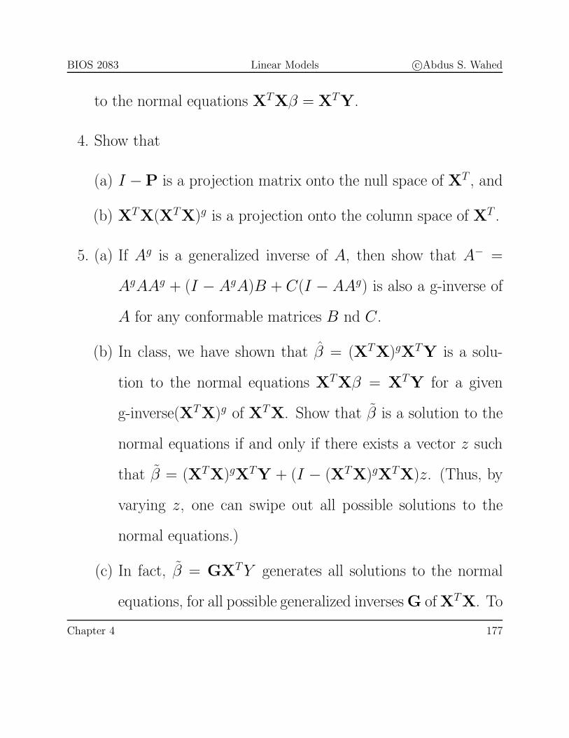
to the normal equations XTXβ = XTY.

4. Show that

(a) I −P is a projection matrix onto the null space of XT , and

(b) XTX(XTX)g is a projection onto the column space of XT .

5. (a) If Ag is a generalized inverse of A, then show that A− =

AgAAg + (I − AgA)B + C(I − AAg) is also a g-inverse of

A for any conformable matrices B nd C.

(b) In class, we have shown that β = (XTX)gXTY is a solu-

tion to the normal equations XTXβ = XTY for a given

g-inverse(XTX)g of XTX. Show that β is a solution to the

normal equations if and only if there exists a vector z such

that β = (XTX)gXTY + (I − (XTX)gXTX)z. (Thus, by

varying z, one can swipe out all possible solutions to the

normal equations.)

(c) In fact, β = GXTY generates all solutions to the normal

equations, for all possible generalized inverses G of XTX. To

Chapter 4 177


show this, start with the general solution β = (XTX)gXTY+

(I − (XTX)gXTX)z (from part (b)). Also take it as a fact

that for a given non-zero vector Y and an arbitrary vector

z, there exists an arbitrary matrix M such that z = MY.

Use this fact, along with the result from part (a) to write β

as GXTY where G is a g-inverse of XTX.

6. For the general one-way ANOVA model,

yij = μ + αi + εij, i = 1, 2, . . . , a; j = 1, 2, . . . , ni,

(a) What is the X matrix?

(b) Find r(X).

(c) Find a basis for the null space of X.

(d) Give a basis for the set of all possible linearly independent

estimable functions.

(e) Give conditions under which c0μ +∑a

i=1 ciαi is estimable.

In particular, is μ estimable? Is α1 − α2 estimable?

Chapter 4 178


(f) Obtain a solution to the normal equation for this problem

and find the least square estimator of αa − α1.

7. Consider the linear model

Y = Xβ + ε, E(ε) = 0, cov(ε) = σ2In. (4.6.1)

Follow the following steps to show that if λTβ is estimable, then

λT β is the BLUE of λTβ, where β is a solution to the normal

equations (XTX)β = XTY.

(a) Consider another linear unbiased estimator c + dtY of λTβ.

Show that c must be equal to zero and dTX = λT .

(b) Now we will show that var(c + dTY) can be written as the

var(λT β) plus some non-negative quantity. To do this, write

var(c + dtY) = var(dTY) = var(λT β + dTY − λT β︸︷︷︸g(Y)

).

Show that g(Y) defined in this manner is a linear function

of Y.

Chapter 4 179


(c) Show that λT β and g(Y) are uncorrelated. Hint: Use

(i) cov(AY, BY) = Acov(Y)BT (ii) Result from part

(b).

(d) Hence

var(c + dTY) = var(dTY) = var(λT β) + . . . .

In other words, variance of any other linear unbiased estima-

tor is greater than or equal to the variance of the least square

estimator.

(e) Show that var(c+dTY) = var(λT β) only if c+dTY = λT β.

8. One example of a simple two-way nested model is as follows. Sup-

pose two instructors taught two classes using Teaching Method I,

and three instructors taught two classes with Teaching Method

II. Let Yijk is the average score for the kth class taught by jth

instructor with ith teaching method. The model can be written

as:

Yijk = μ + αi + βij + εijk.

Chapter 4 180


Assume E(εijk) = 0, and cov(εijk, εi1j1k1) = σ2, if i = i1, j =

j1, k = k1; 0, otherwise.

(a) Write this model as Y = Xβ + ε, explicitly describing the

X matrix and β.

(b) Find r, the rank of X. Give a basis for the null space of X.

(c) Write out the normal equations and give a solution to the

normal equations.

(d) How many linearly independent estimable functions can you

have in this problem? Provide a list of such estimable func-

tions and give the least squares estimators for each one.

(e) Show that the difference in the effect of two teaching methods

is not estimable.

9. Consider the linear model

Yij =i−1∑k=0

βk + εij, i = 1, 2, 3; j = 1, 2; (4.6.2)

with E(εij) = 0; V ar(εij) = σ2; cov(εij, εi′j′) = 0 whenever

i′ �= i or j′ �= j.

Chapter 4 181


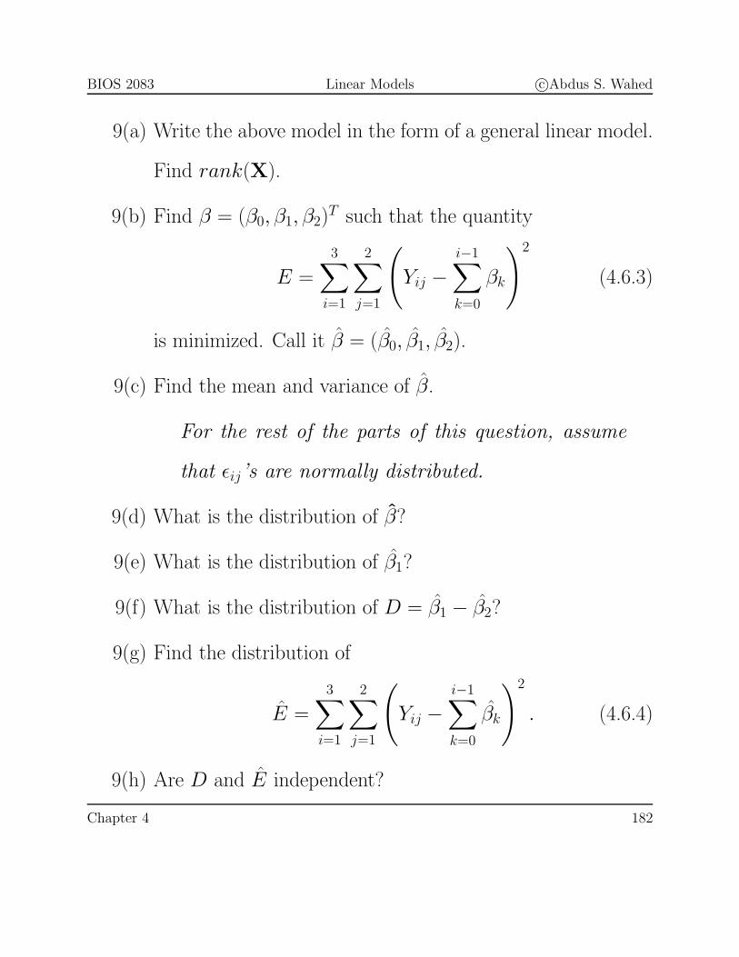
9(a) Write the above model in the form of a general linear model.

Find rank(X).

9(b) Find β = (β0, β1, β2)T such that the quantity

E =

3∑i=1

2∑j=1

(Yij −

i−1∑k=0

βk

)2

(4.6.3)

is minimized. Call it β = (β0, β1, β2).

9(c) Find the mean and variance of β.

For the rest of the parts of this question, assume

that εij’s are normally distributed.

9(d) What is the distribution of β?

9(e) What is the distribution of β1?

9(f) What is the distribution of D = β1 − β2?

9(g) Find the distribution of

E =3∑

i=1

2∑j=1

(Yij −

i−1∑k=0

βk

)2

. (4.6.4)

9(h) Are D and E independent?

Chapter 4 182


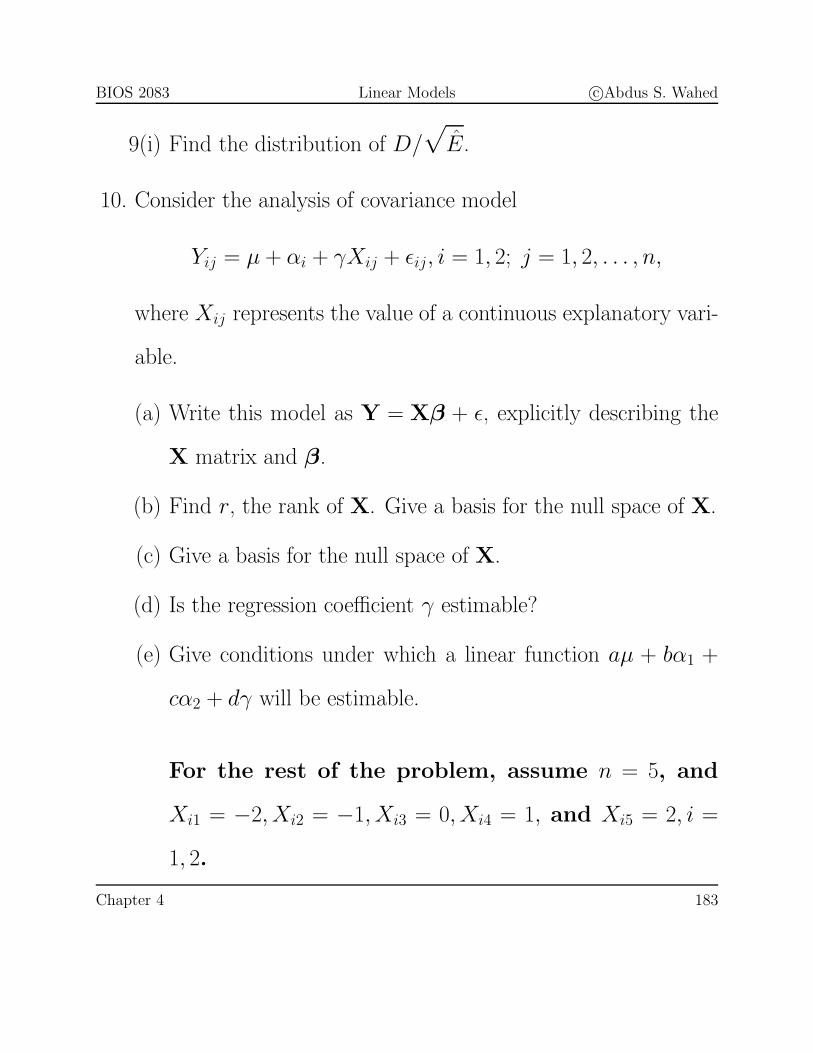
9(i) Find the distribution of D/√

E.

10. Consider the analysis of covariance model

Yij = μ + αi + γXij + εij, i = 1, 2; j = 1, 2, . . . , n,

where Xij represents the value of a continuous explanatory vari-

able.

(a) Write this model as Y = Xβ + ε, explicitly describing the

X matrix and β.

(b) Find r, the rank of X. Give a basis for the null space of X.

(c) Give a basis for the null space of X.

(d) Is the regression coefficient γ estimable?

(e) Give conditions under which a linear function aμ + bα1 +

cα2 + dγ will be estimable.

For the rest of the problem, assume n = 5, and

Xi1 = −2, Xi2 = −1, Xi3 = 0, Xi4 = 1, and Xi5 = 2, i =

1, 2.

Chapter 4 183


(f) Give an expression for the LS estimator of γ and α1 − α2, if

exists.

(g) Obtain the LS estimator of γ under the restriction that α1 =

α2.

(h) Obtain the LS estimator of α1−α2 under the restriction that

γ = 0.

(i) Obtain the LS estimator of γ under the restriction that α1 +

α2 = 0.

11. Consider the two-way crossed ANOVA model with an additional

continuous baseline covariate Xij:

Yij = μi + αj + γXij + εij, i = 1, 2; j = 1, 2; k = 1, 2, (4.6.5)

under usual assumptions (I and II from lecture note). Let the

parameter vector be β = (μ1, μ2, α1, α2, γ)T and X be the cor-

responding X matrix. Define Xi. =∑2

j=1 Xij/2, i = 1, 2 and

X.j =∑2

i=1 Xij/2, j = 1, 2.

(a) Find rank(X).

Chapter 4 184


(b) Give a basis for the null space of X.

(c) Give conditions under which λTβ will be estimable. In par-

ticular:

i. Is γ estimable?

ii. Is μ1 − μ2 estimable?

iii. Is α1 − α2 + γ(X1. − X2.) estimable?

iv. Is μ1 − μ2 + γ(X.1 − X.2) estimable?

v. Is μ1 + γ(X.1 + X.2)/2 estimable?

12. Consider the linear model:

Yijk = βi + βj + εijk, i, j = 1, 2, 3; i < j; k = 1, 2, (4.6.6)

so that there are a total of 6 observations.

(a) Write the model in matrix form and compute the XTX-

matrix.

(b) Write down the normal equations explicitly.

(c) Give condition(s), if any, under which a linear function∑3

i=1 λiβi

is estimable, where λi, i = 1, 2, 3 are known constants.

Chapter 4 185


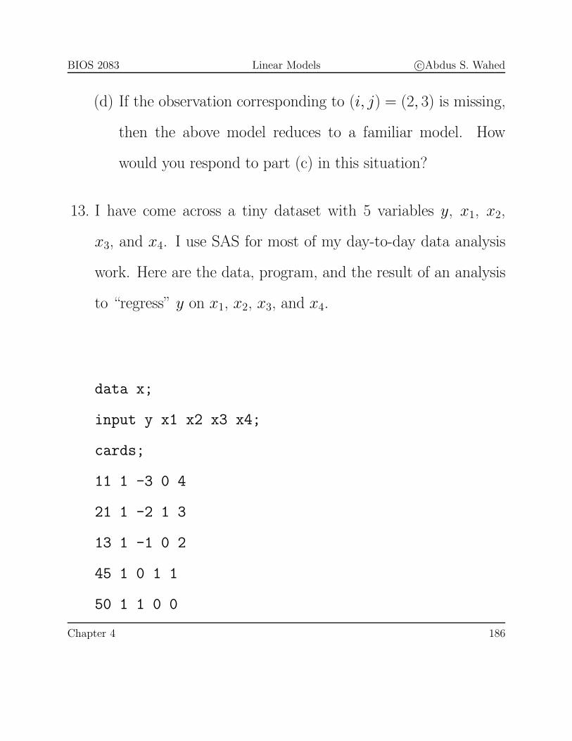
(d) If the observation corresponding to (i, j) = (2, 3) is missing,

then the above model reduces to a familiar model. How

would you respond to part (c) in this situation?

13. I have come across a tiny dataset with 5 variables y, x1, x2,

x3, and x4. I use SAS for most of my day-to-day data analysis

work. Here are the data, program, and the result of an analysis

to “regress” y on x1, x2, x3, and x4.

data x;

input y x1 x2 x3 x4;

cards;

11 1 -3 0 4

21 1 -2 1 3

13 1 -1 0 2

45 1 0 1 1

50 1 1 0 0

Chapter 4 186


;run;

proc glm;

model y=x1 x2 x3 x4/noint solution;

estimate "2b1+b2+b4" x1 2 x2 1 x3 0 x4 1;

estimate "2b1-b2-b3" x1 2 x2 -1 x3 -1 x4 0;

estimate "b1+b2" x1 1 x2 1 x3 0 x4 0;

estimate "b4" x1 0 x2 0 x3 0 x4 1;

estimate "b1+b4" x1 1 x2 0 x3 0 x4 1;

run;

quit;

Output:

========================================

/* Parameter Estimates*/

Parameter Estimate SE t Pr > |t|

x1 34.86666667 B 6.78167465 5.14 0.0358

x2 10.20000000 B 3.25781113 3.13 0.0887

Chapter 4 187


x3 8.33333333 9.40449065 0.89 0.4690

x4 0.00000000 B . . .

/* Contrast Estimates*/

Parameter Estimate SE t Pr > |t|

2b1+b2+b4 79.9333333 15.3958147 5.19 0.0352

b1+b2 45.0666667 8.8221942 5.11 0.0363

b1+b4 34.8666667 6.7816747 5.14 0.0358

I am puzzled by several things I see in the output.

(a) All the parameter estimates except the one corresponding to

x3 has a letter ‘B’ next to it. What explanation can you

provide for that?

(b) What happens to the parameter estimates if you set-up the

model as ‘model y=x2 x3 x4 x1’ or ‘y=x1 x2 x4 x3’? Can you

explain the differences across these three sets of parameter

estimates?

Chapter 4 188


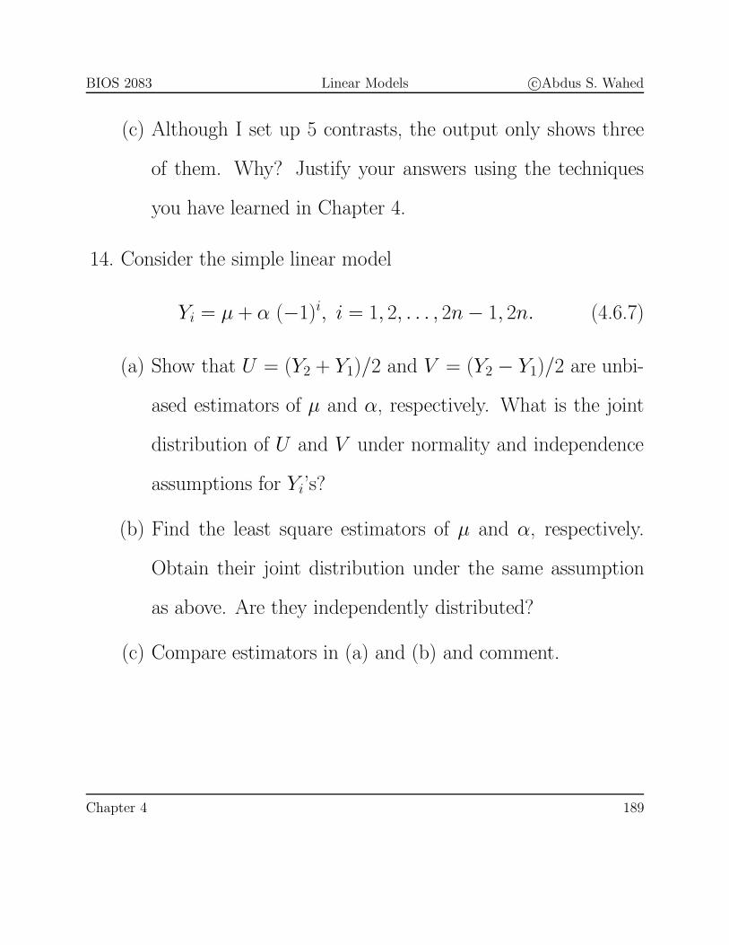
(c) Although I set up 5 contrasts, the output only shows three

of them. Why? Justify your answers using the techniques

you have learned in Chapter 4.

14. Consider the simple linear model

Yi = μ + α (−1)i, i = 1, 2, . . . , 2n − 1, 2n. (4.6.7)

(a) Show that U = (Y2 + Y1)/2 and V = (Y2 − Y1)/2 are unbi-

ased estimators of μ and α, respectively. What is the joint

distribution of U and V under normality and independence

assumptions for Yi’s?

(b) Find the least square estimators of μ and α, respectively.

Obtain their joint distribution under the same assumption

as above. Are they independently distributed?

(c) Compare estimators in (a) and (b) and comment.

Chapter 4 189

chapter 3 112wahed/teaching/2083/fall09/lecture409.pdf · 2009-09-29 · bios 2083 linear models c...

Documents