chapter 3 linear programming - whitman...

$: CHAPTER 3 Linear Programming - Whitman Peoplepeople.whitman.edu/~hundledr/courses/M250F03/ch3.pdf · \chapte 2003/9/ page 2 2 Chapter 3 Linear Programming or the maximum problem max$
“chapte2003/9/page 1

C H A P T E R 3

Linear Programming

Linear programming, like its nonlinear counterpart, is a method for making de-cisions based on solving a mathematical optimization problem. The general fieldof linear programming has been a major area of applied mathematical research inthe last 50 years. A combination of new algorithms, e.g., the simplex method,and widely available computing power now make this an indispensable tool for themathematical modeler.

We begin our discussion of linear programming by presenting the basic math-ematical formulation and terminology in general terms. We will follow this witha number of examples of problems that may be formulated in terms of linear pro-grams. Our goal here is to obtain an abstract understanding of what a linearprogram is and to develop an intuition that will assist the modeler in assessingwhether linear programming is the right tool for a given problem.

Consider a linear function of the variables (x1, . . . , xn),

F (x1, . . . , xn) = f1x1 + f2x2 + · · ·+ fnxn

where the parameters fi are known. We seek to pick the values of all the xi, referredto as decision variables, so as to maximize F (x1, . . . , xn) which is referred to as theobjective function. Clearly picking each xi = ∞ (or even just one) would providea maximum, albeit meaningless. The interest arises when the values of the xi areconstrained, e.g.,

a11x1 + · · ·+ a1nxn ≤ b1

Based on the application many constraints are possible so we write

ai1x1 + · · ·+ ainxn ≤ bi

for i = 1, . . . , m. Note that these constraints are also linear in the decision variables.We may interpret this system of constraints geometrically as defining a region, i.e., acontinuum of points such that all the constraints are simultaneously satisfied. Thisregion is referred to as the feasible set S. So we may view the optimization problemas one to find the maximum value of the objective function over the feasible set S.

We now formulate this optimization problem in terms of vectors and matrices.Let x = (x1, . . . , xn)T be the (column) vector of the unknown variables, and letf = (f1, . . . , fn)T be the vector of coefficients of the objective function, F (x) = fT x.We also introduce the m × n matrix A whose entries are the coefficients in theinequality constraints, (A)ij = aij . If a and b are vectors of the same length thenwe write a ≥ b if ai ≥ bi holds for all components.

Definition 1. A linear program associated with f , A, and b is the minimumproblem

minx

fT x

1


2 Chapter 3 Linear Programming

or the maximum problemmax

xfT x

subject to the constraintAx ≤ b.

3.1 EXAMPLES OF LINEAR PROGRAMS

In this section we survey a variety of applications that fit exactly into the formulation ofthe abstract linear program.

3.1.1 Red or White?

A winemaker would like to decide how many bottles of red wine and how manybottles of white wine to produce. Given his expertise is in red wine making he cansell a bottle of red wine for $12 while he can only sell a bottle of white wine for$7. Clearly the winemaker would seek to maximize his profits, and, having recentlycompleted a course in mathematical modeling, proceeds to construct the objectivefunction

F (x1, x2) = 12x1 + 7x2

where the decision variables are the number of bottles of red wine to produce x1

and the number of bottles of white wine to produce, i.e., x2.Aging wine in wooden or glass-lined vats is an integral component of the

production process, but due to limited space the wine must be aged for a limitedtime. The wine maker has determined that red wine should be aged two years perbottle and white wine one year per bottle and his facilities allow that each batch islimited to 10,000 bottle-years (5 bottles of red and 3 bottles of white require a totalof 13 bottle years ripening time). Thus the winemaker formulates a constraint

2x1 + x2 ≤ 10000

Also the volume of grapes that may be processed is limited and it takes 3gallons of grapes to make a bottle of red wine and two gallons of grapes to makea bottle of white wine. Furthermore, the winery can only process a total of 16,000gallons of grapes for each batch. Thus, the winemaker produces the additionalconstraint

3x1 + 2x2 ≤ 16000

Now the winemaker would like to determine how many bottles of each wineto produce as well as how much money he will expect to make. Note that we mustalso require that negative bottles of wine are not allowed so

x1 ≥ 0

andx2 ≥ 0


Section 3.2 Geometric Solution of a 2D Linear Program 3

3.1.2 How Many Fish?

A child with a new 29 gallon fish tank asks her daddy to put as many fish in thetank as possible. Sensing that too many fish is not a good thing, the dad asks thepet shop owner how many fish can go into a tank. The answer was more complexthan anticipated. ”You can put one inch of fish in per gallon of water.” The littlegirl then added that she wanted only the big orange fish (Gouramis) and the smallstripy fish (Zebra Danios).

As the child seeks to maximize the total number of fish her objective functionis

F (x1, x2) = x1 + x2

where x1 is the number of Gouramis and x2 is the number of Zebra Danios.Additionally, a full grown Gourami is two inches long while a Danio is just

one inch long. The constraint of not exceeding 29 inches of total fish length cannow be written

2x1 + x2 ≤ 29

Danios are very active fish and actually require twice as much food as Gouramis.Each Danio eats 4 grams/day of fish flakes while the slower Gourami eats 2 grams/day.The dad decides that he would prefer not to go broke buying fish food and thuswants to limit the tank to 50 grams/day. Thus, we have the constraint

2x1 + 4x2 ≤ 50

The pet shop owner adds, by the way, that Danios need to live in schools ofat least 5 fish or they don’t do well. Thus

x2 ≥ 5

Additionally, the little girl stipulates that she must have at least two Gouramisas they are known to kiss (hence the term Kissing Gouramis) so we add

x1 ≥ 2

How many Gouramis and Danios can the little girl have in her tank?

3.2 GEOMETRIC SOLUTION OF A 2D LINEAR PROGRAM

Let us now solve the winemaker’s linear programming problem using graphicaltechniques. Recalling the problem:

• Objective function: F (x1, x2) = 12x1 + 7x2

• Constraint 1: 3x1 + 2x2 ≤ 16000

• Constraint 2: 2x1 + x2 ≤ 10000

• Constraint 3: x1 ≥ 0




0 1000 2000 3000 4000 5000 60000

2000

4000

6000

8000

10000

12000

number of bottles of red wine

Red versus White

num

ber

of b

ottle

s of

whi

te w

ine

Isoprofit lines

FEASIBLE REGION

(4000, 2000)

Constraints

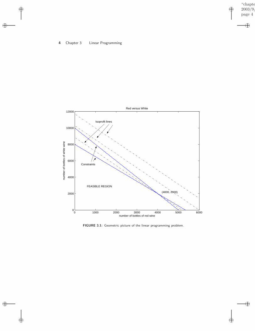
FIGURE 3.1: Geometric picture of the linear programming problem.


Section 3.3 Sensitivity Analysis 5

First, let us identify the feasible set. Again, this is the intersection of allthe regions defined by the constraints. (Note that this set is independent of theobjective function.) The boundary of the first constraint is defined by the equality

x2 = 8000− 32x1

The constraint may be viewed as a half-plane with this line dividing the regionof allowed points from the unallowed points. It is easy to identify which regionis the allowed region by considering a single point. For example, is the origin apoint that satisfies the first constraint? Since the answer is clearly yes we knowthat the set of points that satisfies constraint 1 consists of the halfplane defined byx2 = 8000− 3

2x1 that contains origin.Similarly, the second constraint defines a halfplane of points containing the

origin and bounded by the line

x2 = 10000− 2x1

The intersection of constraints 3 and 4 is the first quadrant of the x1x2 plane.The intersection of all of these constraints as shown in Figure 3.1 constitutes

the feasible set. Now we must pick the point in the feasible set that maximizes theobjective function.

We can define an isoprofit line to be

12x1 + 7x2 = c

For all points on this line the profit is the same. We can see that as c decreasesthe line shifts towards the origin. So the goal is to pick the isoprofit line with thelargest value of c such that x1, x2 is a point in the feasible set. Graphically wesee that the first point the descending isoprofit line will touch is the vertex of theintersection of constraints 1 and 2. This is easily calculated to be (4000, 2000).

Thus, the solution to the winemaker’s linear programming problem is that heshould produce 4000 bottles of red and 2000 bottles of white and that this will leadto a maximum profit of $62,000.

3.3 SENSITIVITY ANALYSIS

Often the coefficients in a linear programming model are known only approximately.Thus, it is interesting to know what the impact of modifying the terms present inthe model. How is the objective function impacted? How does the optimal solutionchange? These questions are the subject of sensitivity analysis.

3.3.1 Price Sensitivity

First we examine how changing the price of a bottle of white wine impacts theoptimal solution. Letting the price of the white wine be a variable w we now havethe linear program

• Objective function: F (x1, x2) = 12x1 + wx2

• Constraint 1: 3x1 + 2x2 ≤ 16000



• Constraint 2: 2x1 + x2 ≤ 10000



From our graphical solution we know that any isoprofit line with slope between -2and -3/2 will produce the same optimal solution of (4000, 2000). Since the slope ofthe isoprofit line is −12/w this condition is

−2 <12w

< −32

from which we conclude that the price of the white wine may vary as

6 < w < 8

with the solution unchanged as (4000, 2000). Further examination produces Table3.1. The double arrows here mean that any point on the isoprofit curve containingthese points produces the same profit.

cost of white wine optimal solution6 < w < 8 (4000, 2000)

w = 6 (4000, 2000)↔ (5000, 0)w = 8 (4000, 2000)↔ (0, 8000)w < 6 (5000, 0)w > 8 (0, 8000)

TABLE 3.1: The effect of pricing the white wine on the optimal solution.

3.3.2 Resource Sensitivity

Now we let the number of gallons of grapes, α, and the number of bottle-yearsstorage capacity, β, be variable. Now the linear program becomes


• Constraint 1: 3x1 + 2x2 ≤ α

• Constraint 2: 2x1 + x2 ≤ β



The relative values of α and β determine the geometry of the solution. For ex-ample, if α/2 > β then constraint 1 becomes irrelevant. When the intersection ofconstraints 1 and 2 determines the optimal solution it is readily shown that

x1 = −α + 2β


Section 3.4 Linear Programs with Equality Constraints 7

andx2 = 2α− 3β

Hence the optimal solution to the objective function can be expressed as

f(x1, x2) = 2α + 3β

Consequently, if α is increased by one unit then f(x1, x2) is increased by 2, while if βis increased by one unit then f(x1, x2) is increased by 3. So if a winemaker considersexpanding his winery he realizes that the cost of increasing grape processing mustbe less than $2 and the expense of increasing wine storage must be less than $3.Otherwise expansion will lose money.

3.3.3 Constraint Coefficient Sensitivity

Now we consider the problem of adjusting one of the coefficients in one of theconstraint equations. In particular consider the amount of time γ we age a bottleof red wine to be allowed to vary.


• Constraint 1: 3x1 + 2x2 ≤ 16000

• Constraint 2: γx1 + x2 ≤ 10000



To simplify the discussion, let’s examine the effect of reducing the amount of timewe age the red wine from 2 years to 1.95 years. The solution to the resulting linearprogram suggests that now 4444 bottles of red can be sold while 1333 bottles ofwhite can be sold for a total profit of $62,659, increasing the income by almost$700. Of course, for this to be advisable it must be true that all the bottles ofthis ”younger” red wine can still be sold at the same price, i.e., the taste has notsuffered enough to reduce its popularity.

3.4 LINEAR PROGRAMS WITH EQUALITY CONSTRAINTS

In the examples treated so far the constraints defining the feasible sets have beeninequalities. However, in practice it is often the case that further constraints in theform of equalities have to be met.

Definition 2. Let f be a column vector of length n, b a column vector oflength m, and beq a column vector of length k. Let further A and Aeq bem× n and k × n matrices, respectively. A linear program associated with f ,A, b, Aeq and beq is the minimum problem

minx

fT x (3.1)

or the maximum problemmax

xfT x (3.2)



subject to the constraints

Ax ≤ bAeqx = beq.

(3.3)

3.4.1 A Task Scheduling Problem

A steel manufacturer produces four different sizes Si, 1 ≤ i ≤ 4 (small, medium,large, and extra large), of beams. These beams can be produced on any one ofthree machines Mj, 1 ≤ j ≤ 3. Machine Mj produces lij feet of the beams of sizeSi per hour. Each machine can be used up to 50 hours per week and the hourlyoperating cost of machine Mj is $cj . The manufacturer has to produce ki feet ofbeams of size Si per week. We assume that lij , cj and ki are given numbers.

Clearly the manufacturer wants to minimize the total operating costs. Toformulate this minimization problem as a linear program, let xij be the number ofhours per week machine Mj produces the beams of size Si. The total operatingcosts are

F (x) =3∑

j=1

4∑i=1

cjxij =

c1(x11 + x21 + x31 + x41)+c2(x12 + x22 + x32 + x42)+c3(x13 + x23 + x33 + x43)

(3.4)

and this function has to be minimized subject to the following constraints:

• Each machine can operate at most 50 hours per week. Thus the variables xij

have to satisfy the inequalities

x1j + x2j + x3j + x4j ≤ 50 (1 ≤ j ≤ 3). (3.5)

• Since xij cannot be negative we have to introduce twelve further inequalityconstraints

−xij ≤ 0 (1 ≤ i ≤ 4, 1 ≤ j ≤ 3). (3.6)

• The number of feet of the beams of size Si produced per week by machineMj is lijxij . Thus the total number of feet of this size produced in a week is∑

j lijxij , and this must be equal to

li1xi1 + li2xi2 + li3xi3 = ki (1 ≤ i ≤ 4). (3.7)

We now have a linear program with fifteen inequality constraints and four equalityconstraints.

To match the steel manufacturer problem to Definition 2, we write the twelvevariables in a column vector,

x = [x11, x21, x31, x41, x12, x22, x32, x42, x13, x23, x33, x43]T .

The inequality constraints (3.5) and (3.6) have to be written in matrix vectorform as Ax ≤ b. Let us denote by A1 and b1 the 3×12–matrix and the column vector


Section 3.4 Linear Programs with Equality Constraints 9

of length 3, respectively, such that the inequalities (3.5) take the form A1x ≤ b1,i.e.

A1 =

1 1 1 1 0 0 0 0 0 0 0 0

0 0 0 0 1 1 1 1 0 0 0 00 0 0 0 0 0 0 0 1 1 1 1

, b1 =

50

5050

.

The inequalities (3.6) can be written as A2x ≤ b2, where A2 = −I with I the12 × 12–identity matrix, and b2 the column vector of length twelve whose entriesare all zero. Thus the diagonal entries of A2 are −1 and the other entries are zero.

The full 15× 12–matrix A is then obtained by appending the twelve rows ofA2 below the three rows of A1 and similarly for b,

A =

1 1 1 1 0 0 0 0 0 0 0 00 0 0 0 1 1 1 1 0 0 0 00 0 0 0 0 0 0 0 1 1 1 1

−1 0 0 0 0 0 0 0 0 0 0 00 −1 0 0 0 0 0 0 0 0 0 00 0 −1 0 0 0 0 0 0 0 0 00 0 0 −1 0 0 0 0 0 0 0 00 0 0 0 −1 0 0 0 0 0 0 00 0 0 0 0 −1 0 0 0 0 0 00 0 0 0 0 0 −1 0 0 0 0 00 0 0 0 0 0 0 −1 0 0 0 00 0 0 0 0 0 0 0 −1 0 0 00 0 0 0 0 0 0 0 0 −1 0 00 0 0 0 0 0 0 0 0 0 −1 00 0 0 0 0 0 0 0 0 0 0 −1

, b =

505050000000000000

.

Likewise, setting

Aeq =

l11 0 0 0 l12 0 0 0 l13 0 0 00 l21 0 0 0 l22 0 0 0 l23 0 00 0 l31 0 0 0 l32 0 0 0 l33 00 0 0 l41 0 0 0 l42 0 0 0 l43

, beq =

k1

k1

k3

k4

,

the equality constraints (3.7) can be written in the form Aeqx = beq.

3.4.2 Transportation Problems

Transportation problems are typical applications of linear programming. Assumea company has storage depots at m different locations A1, . . . , Am in which k dif-ferent products P1, . . . , Pk are stored. Let Mij be the total amount of product Pj

stored in depot Ai. The company has customers C1, . . . , Cr in r different citiesand has to deliver the amount Nlj of product Pj to customer Cl. We assume fixedtransportation costs Tilj per unit amount of product Pj if transported to customerCl from storage deposit Ai.

Let xilj be the amount of product Pj delivered to customer Cj from deposit



Ai. The problem is to minimize the total transportation costs

m∑i=1

r∑l=1

k∑j=1

Tiljxilj = min

subject to the constraints

xilj ≥ 0 for 1 ≤ l ≤ r, 1 ≤ j ≤ k, 1 ≤ i ≤ m (3.8)r∑

l=1

xilj ≤ Mij for 1 ≤ i ≤ m, 1 ≤ j ≤ k (3.9)

m∑i=1

xilj = Nlj for 1 ≤ l ≤ r, 1 ≤ j ≤ k. (3.10)

This is clearly a linear programming problem with inequality constraints (3.8) and(3.9) and equality constraints (3.10). If m, k, r and the numbers Tilj , Mij , Nlj aregiven, the vectors and matrices f, A, b, Aeq, beq can be constructed similarly as inSubsection 3.4.1.

3.5 A TARGETING PROBLEM

Consider the following problem of launching a rocket to a fixed altitude h in a giventime T , while expending a minimum amount of fuel. Let a(t) be the accelerationexerted, y(t) the rocket altitude, and v(t) the rocket velocity at time t. The problemcan be formulated as follows.

Minimize∫ T

0 |a(t)|dt

Subject to dv(t)dt = a(t)− g, dx(t)

dt = v(t)y(T ) = hy(t) ≥ 0 (0 ≤ t ≤ T )y(0) = 0, v(0) = 0|a(t)| ≤ a0 (0 ≤ t ≤ T ),

(3.11)

where a0 is the maximal acceleration that can applied due to power limitations.Clearly in order that the rocket can leave the ground a0 must be greater than theearth acceleration g.

Note that the maximum altitude hmax to which the rocket can be launchedis reached if a(t) = a0 for 0 ≤ t ≤ T . If h > hmax then (3.11) has no solution. Byintegrating the equations for dv(t)/dt and dy(t)/dt in (3.11) we find

hmax = (a0 − g)T 2/2.

3.5.1 Discretization and Solution of the Equations of Motion

Equation (3.11) belongs to the class of continuous optimization problems which doesnot fit a priori into the class of linear programming problems. In order to make theproblem amenable to linear programming, we discretize time and assume that

a(t) = ai = const for ti−1 < t < ti, (3.12)


Section 3.5 A Targeting Problem 11

whereti = iτ τ = T/n,

and n is a positive integer. The discretized problem is described by n variables(a1, . . . , an) which have to be determined.

Within each of the n sub-intervals into which the interval 0 ≤ t ≤ T is divided,the rocket encounters a constant acceleration,

dv(t)dt

= ai − g,dx(t)

dt= v(t) if ti−1 ≤ t ≤ ti. (3.13)

After integration these equations lead to the well known linear and quadratic timedependence of velocity and altitude in each sub-interval,

v(t) = (ai − g)(t− ti−1) + v(ti−1) (3.14)

y(t) =12(ai − g)(t− ti−1)2 + v(ti−1)(t− ti−1) + y(ti−1). (3.15)

We now setvi = v(ti), yi = y(ti) (1 ≤ i ≤ n),

and evaluate the equations (3.14) and (3.14) at t = ti to obtain

vi = (ai − g)τ + vi−1

yi = 12 (ai − g)τ2 + vi−1τ + yi−1.

(3.16)

Equation (3.16) is a linear system of first order difference equations for the (vi, yi).The initial values are (v0, y0) = (0, 0). Methods for solving difference equations arediscussed in Chapter 6, and we will show there that the solution of (3.16) is givenby

vi = τ( i∑

j=1

aj − ig)

(3.17)

yi = τ2( i∑

j=1

(12

+ i− j)aj − i2g

2

). (3.18)

These equations form the solution of the discretized equations of motion for anygiven set of acceleration values (a1, . . . , an).

3.5.2 Formulation as Linear Program

Now we formulate the discretized optimization problem as linear programmingproblem with inequality and equality constraints. The equations of motion

dv(t)dt

= a(t)− g,dx(t)

dt= v(t), y(0) = 0, v(0) = 0 (3.19)

have been solved already, so we only need to consider the equality and inequalityconstraints

y(T ) = h, |a(t)| ≤ a0, y(t) ≥ 0 (0 < t < T ).



From equation (3.18) we infer that the discretized forms of the equality and in-equality constraints for y(t) (note that y(T ) = yn) can be written as

n∑j=1

(12

+ n− j)aj =

n2g

2+

h

τ2(3.20)

i∑j=1

(12

+ i− j)aj ≥ i2g

2, (1 ≤ i ≤ n− 1), (3.21)

and the constraint for a(t) becomes

|ai| ≤ a0 (1 ≤ i ≤ n). (3.22)

The objective function which has to be minimized in the discretized problem is

n∑i=1

|ai| = min, (3.23)

and the minimization is subject to the constraints (3.20)– (3.22).Note that (3.22) and (3.23) involve the absolute values of the variables ai and

hence are not described by linear functions. For inequalities this is not a problem,however there is no way to rewrite the objective function (3.23) as a linear function∑

i fiai. To solve this problem we treat the absolute values as extra variables. Ourminimization problem then depends on 2n unknown variables which we write againin a column vector

x = [x1, . . . , xn, xn+1, . . . , x2n]T ,

wherexi = ai, xi+n = |ai| (1 ≤ i ≤ n).

The objective function is now a linear function of x,

F (x) =2n∑

i=n+1

xi = min . (3.24)

In order that the conditions xi+n = |xi| are met we have to introduce addi-tional constraints. Since ai ≤ |ai| and −ai ≤ |ai| we impose

xi ≤ xi+n

−xi ≤ xi+n

}for 1 ≤ i ≤ n. (3.25)

Clearly the inequalities (3.25) are not equivalent to the condition xi+n = |xi|.However it can be shown that the solution of any linear programming problem islocated on the boundary of the feasible set, and for our problem this necessarilyimplies that for each i one of the two inequalities in (3.25) turns into an equality ifx is an optimal solution.



The inequality and equality constraints (3.20)–(3.22) are now rewritten interms of the xi as

xn+i ≤ a0 for 1 ≤ i ≤ n (3.26)

−i∑

j=1

(12

+ i− j)xj ≤ − i2g

2for 1 ≤ i ≤ n− 1 (3.27)

n∑j=1

(12

+ n− j)xj =

n2g

2+

h

τ2. (3.28)

The discretized optimization problem is now to minimize the objective functionF (x) in (3.24) subject to the inequality constraints (3.25)–(3.27) and the equalityconstraint (3.28). The objective function as well the inequality and equality con-straints are formulated in terms of linear functions of x and so match the abstractproblem (3.1) subject to the constraints (3.3) of Definition 2. The matrix A is a(4n− 1)× 2n matrix and Aeq is a 1× 2n matrix, i.e. a row vector.

Numerical Solutions. In Figure 3.2 we show the optimal acceleration functiona(t) obtained by numerical solution of (3.24)–(3.28) together with v(t) and y(t) forn = 5 (Figure 3.2 (a)) and n = 25 (Figure 3.2 (b)), and h = 300 and h = 700.The other paramters are fixed at g = 32, T = 10, and a0 = 48. The optimalsolution has been computed using the linprog command of Matlab. The procedurefor generating the plots in Figure 3.2 can be summarized as follows.

• Generate the matrices and vectors f , A, b, Aeq , and beq of the linear programaccording to equations (3.24)–(3.28).

• Apply a numerical solver to find the solution vector x. The first n componentsof x are the optimal acceleration values (a1, . . . , an).

• Apply equations (3.17) and (3.18) to compute the velocity and altitude vectors(v1, . . . , vn) and (y1, . . . , yn).

• Use equations (3.12), (3.14) and (3.15) to compute the piecewise constant,piecewise linear and piecewise quadratic functions a(t), v(t) and y(t).

• Plot a(t), v(t), y(t).

As can be seen in Figure 3.2 the optimal acceleration and altitude functionsshow some distinct features. The acceleration function a(t) starts with a0 andstays there over a certain number of sub–intervals, then it decreases in the nextsub–interval, and after that a(t) is zero. The altitude function y(t) is monotonicallyincreasing and reaches the target altitude from below for larger values of h, whereasfor smaller values of h it passes through a maximum and reaches the target altitudefrom above. In Section 3.6 we will see that the optimal solution to the discretizedtargeting problem is the best approximation of a known analytical solution to (3.11).



0 2 4 6 8 100

10

20

30

40

50

t

a(t)

h=300

h=700

0 2 4 6 8 10−100

−50

0

50

100

150

t

v(t)

h=700

h=300

0 2 4 6 8 100

200

400

600

800

t

y(t)

h=700

h=300

(a)

0 2 4 6 8 100

10

20

30

40

50

t

a(t)

h=300

h=700

0 2 4 6 8 10−100

−50

0

50

100

150

t

v(t)

h=700

h=300

0 2 4 6 8 100

200

400

600

800

t

y(t)

h=700

h=300

(b)

FIGURE 3.2: Graphs of a(t), v(t), y(t) obtained by numerical solution of the linear program (3.24)–(3.28) for g = 32, T = 10, a0 = 48, and two heights h = 300 and h = 700. (a): n = 25, (b):n = 5.



3.5.3 Targeting Problem with Air Resistance

Air resistance is modeled by a friction force Fd(v). Since linear programming re-quires a linear model we assume Fd(v)/m = −kv, where k is a friction coefficientin which the mass is absorbed. The problem (3.11) remains the same except thatthe equation for dv(t)/dt is now replaced by

dv(t)dt

= a(t)− g − kv(t). (3.29)

Discretization and Solution of the Equations of Motion. Equation (3.29)is a linear first order differential equation for v(t). In a later chapter we will seethat the solution of (3.29) in the interval ti−1 ≤ t ≤ ti, where a(t) = ai = const, isgiven by

v(t) =ai − g

k+

(v(ti−1)− ai − g

k

)(1− e−k(t−ti−1)

). (3.30)

The altitude y(t) still satisfies dy(t)/dt = v(t) and so can be found by integrationof (3.30),

y(t) = y(ti−1) +ai − g

k

(t− ti−1

)+

1k

(v(ti−1)− ai − g

k

)(1− e−k(t−ti−1

). (3.31)

Evaluating (3.30) and (3.31) at t = ti and letting again vi = v(ti), yi = y(ti) yields

vi = pai − gp + qvi−1

yi = rai − gr + pvi−1 + yi−1,(3.32)

where we have set

q = e−kτ , p = (1− q)/k, r = (τ − p)/k.

Equations (3.32) form again a linear system of first order difference equations. Thissystem is more complicated than (3.16), but still can be solved using the methodsof Chapter 6. The solution is

vi = pi∑

j=1

qi−jaj − gp(1− qi)1− q

(3.33)

yi =i∑

j=1

(r +

p2(1− qi−j)1− q

)aj − gp2(i− 1− ig + qi)

(1− q)2− igr. (3.34)

Formulation as Linear Program. The formulation of the discretized targetingproblem with friction as linear program proceeds in the same way as in Subsection3.5.2. We introduce the vector x of variables xi = ai and xi+n = |ai| (1 ≤ i ≤ n),the objective function (3.24), and the inequality constraints (3.25)–(3.27). Theconstraints yi ≥ 0 for 1 ≤ i ≤ n− 1 and yn = h become

−i∑

j=1

(r +

p2(1− qi−j)1− q

)xj ≤ −gp2(i− 1− iq + qi)

(1− q)2− igr (3.35)

n∑j=1

(r +

p2(1− qn−j)1− q

)xj =

gp2(n− 1− nq + qn)(1 − q)2

+ ngr + h. (3.36)



0 2 4 6 8 100

25

50

t

a(t)

k=0.1

k=0.4

0 2 4 6 8 10−60

−40

−20

0

20

40

60

80

t

v(t)

k=0.1

k=0.4

0 2 4 6 8 100

150

300

t

y(t)

k=0.1

k=0.4

(a)

0 2 4 6 8 100

20

40

t

a(t)

k=0.1

k=0.4

0 2 4 6 8 10−60

−40

−20

0

20

40

60

80

t

v(t)

k=0.1

k=0.4

0 2 4 6 8 100

100

200

300

t

y(t)

k=0.1

k=0.4

(b)

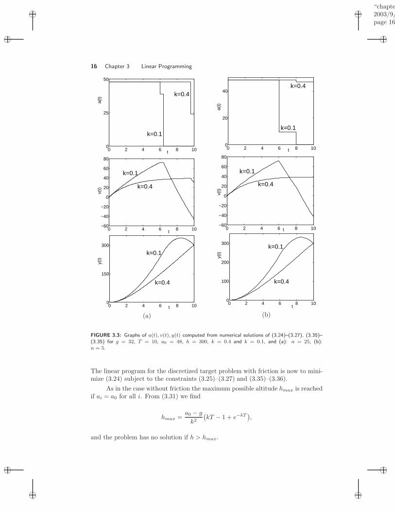
FIGURE 3.3: Graphs of a(t), v(t), y(t) computed from numerical solutions of (3.24)–(3.27), (3.35)–(3.35) for g = 32, T = 10, a0 = 48, h = 300, k = 0.4 and k = 0.1, and (a): n = 25, (b):n = 5.

The linear program for the discretized target problem with friction is now to mini-mize (3.24) subject to the constraints (3.25)–(3.27) and (3.35)–(3.36).

As in the case without friction the maximum possible altitude hmax is reachedif ai = a0 for all i. From (3.31) we find

hmax =a0 − g

k2

(kT − 1 + e−kT

),

and the problem has no solution if h > hmax.


Section 3.6 Analysis of the Targeting Problem 17

Numerical Solutions. In Figure 3.3 we show the graphs of a(t), v(t), and y(t)computed from numerical solutions of the linear program (3.24)–(3.27), (3.35)–(3.36) for g = 32, T = 10, a0 = 48, h = 300, k = 0.4 and k = 0.1, and n = 25and n = 5. The solutions are similar to those for the problem without friction, andclearly the greater k the greater is the fuel consumption.

3.5.4 Additional Constraints

There is no problem to impose further conditions on the optimal solution of thetargeting problem (with or without friction), provided these conditions can be for-mulated as linear equality or inequality constraints. We describe two such condi-tions.

Soft Landing. Soft landing means that the target altitude is reached with veloc-ity v(T ) = 0. This condition can be build into the linear program by imposing theadditional equality constraint

vn = 0,

where vn is represented in terms of the aj = xj through equations (3.17) for k = 0 or(3.33) for k > 0. The vector beq then becomes a vector of length 2, and accordinglyAeq is a 2× 2n–matrix.

Upper Bound for the Velocity. To avoid damage it may be necessary to re-strict also the magnitude of the velocity to |v(t)| ≤ v0. For the discretized problemthis requires that |vi| ≤ v0 for 1 ≤ i ≤ n. This inequality is equivalent to the twolinear inequalities

vi ≤ v0, −vi ≤ v0.

When the vi are represented in terms of the xi, these conditions take the form of 2nadditional linear inequality constraints imposed on x. The vector b is then extendedto a vector of length 6n−1, and accordingly A is extended to a (6n−1)×2n–matrix.

Numerical Solutions. In Figure 3.4 the graphs of a(t), v(t), and y(t) computedfrom the optimal solution of the targeting problem with the condition of soft landingare shown for g = 32, T = 20, a0 = 80, h = 400, k = 0.4, and n = 5. Figure 3.4 (b)was obtained with the additional inequality constraint |v(t)| ≤ 30.

We note that the targeting problem with one of the additional constraintsconsidered in this subsection does not admit easily accessible analytical solutions.In contrast, without these additional constraints analytical solutions can be easilyfound as will be shown in the next section.

3.6 ANALYSIS OF THE TARGETING PROBLEM

In this section we study the targeting problem (3.11) analytically. The numericalsolutions shown in Figure 3.2 suggest that the optimal acceleration function a(t) ismaximal in a certain initial interval 0 ≤ t ≤ T1 and zero for T1 < t ≤ T , where T1

is adjusted such that the target altitude h is reached in time T . We will see thatfor this acceleration function the fuel consumption is indeed minimal.



0 10 20

40

60

t

a(t)

0 10 20

0

30

60

t

v(t)

0 10 200

200

400

t

y(t)

(a)

0 10 2025

35

45

t

a(t)

0 10 20

0

15

30

t

v(t)

0 10 200

200

400

t

y(t)

(b)

FIGURE 3.4: Graphs a(t), v(t), y(t) computed from the optimal solution of the discretized targetingproblem for g = 32, T = 20, a0 = 80, h = 400, k = 0.4, and n = 5, with additional constraints (a):v(T ) = 0, (b): v(T ) = 0 and |v(t)| ≤ 30.



3.6.1 Analytical Solution

Let a(t) be an acceleration function of the form

a(t) ={

a0 if 0 ≤ t ≤ T1

0 if t > T1,(3.37)

where a0 > g and T1 > 0 are given numbers. For this form the solution of theequations of motion (3.19) is given by (Exercise 3.11 (a))

v(t) ={

(a0 − g)t if 0 ≤ t ≤ T1

a0T1 − gt if t ≥ T1,(3.38)

y(t) ={

(a0 − g)t2/2 if 0 ≤ t ≤ T1

−a0T21 /2 + a0T1t− gt2/2 if t ≥ T1.

(3.39)

Consider then the problem of launching the rocket to a prescribed altitude h in agiven time T . The condition y(T ) = h leads to the quadratic equation

−12a0T

21 + a0T1T − 1

2gT 2 = h

for T1. The solution with T1 ≤ T is

T1 = T(1−

√1− (g + 2h/T 2)/a0

), (3.40)

and in order that the expression under the square root be positive we have to requirethat

h ≤ (a0 − g)T 2/2. (3.41)

If T1 and a0 are related by (3.40), the fuel consumption measured by C =∫ T

0 a(t)dt = a0T1 is

C = a0T(1−

√1− (g + 2h/T 2)/a0

). (3.42)

The following theorem (Exercise 3.11 (c)) shows that C is the minimal fuel con-sumption that can be achieved if |a(t)| is bounded by a0.

Theorem 3. Let a(t) be an arbitrary piecewise constant acceleration functionsuch that y(T ) = h for the solution of (3.19), and assume that |a(t)| ≤ a0.Then (3.41) is satisfied, and

∫ T

0

|a(t)|dt ≥ C,

where C is given by equation (3.42).

Thus the solution of the original (not discretized) targeting problem (3.11) is givenby (3.37) with T1 and a0 related by (3.40), provided the inequality (3.41) is satisfied.The expression (a0−g)T 2/2 on the right hand side of this inequality is the maximalaltitude to which the rocket can be launched in time T if |a(t)| is bounded by a0.This altitude is reached if T1 = T , i.e. for the uniform acceleration a(t) = a0 for



0 ≤ t ≤ T . If h > (a0 − g)T 2/2 then a solution to the targeting problem (3.11)does not exist.

When a numerical solver is applied to the linear program of Subsection 3.5.2,the solver seeks to find the best approximation to the analytical solution (3.37),(3.40). The best approximation is

a(t) =

a0 if 0 ≤ t < mτa1 < a0 if mτ ≤ t ≤ (m + 1)τ

0 if t ≥ (m + 1)τ,

where m is the largest integer for which mτ ≤ T1(a0). The value of a1 is adjustedsuch that the altitude h is reached from the initial data (v(mτ), y(mτ)) within time(n−m)τ . In the unlikely case that T1/τ is an integer, the discrete optimal solutioncoincides with the exact optimal solution.

3.6.2 Dimensionless Variables

Equation (3.40) depends on the physical variables T1, T, h, g, a0. We could applydimensional analysis to reduce the number of variables, but there is a simpler wayto identify the relevant dimensionless combinations. If (3.40) is divided by T , theequation can be rewritten as

θ = 1−√

1− 1/β, (3.43)

whereθ =

T1

T≤ 1, β =

a0

g + 2h/T 2≥ 1. (3.44)

The variable θ is the ratio of T1 and T and so θ ≤ 1. The denominator in β is theuniform acceleration (active for 0 ≤ t ≤ T ) through which the rocket is launched tothe target altitude h in time T . According to (3.41) h + gT 2/2 ≤ a0, hence β ≥ 1.

A natural dimensionless variable in terms of which the fuel consumption canbe measured is the ratio

γ = C/C0, (3.45)

where C0 is the fuel consumption for the uniform acceleration g + 2h/T 2,

C0 = (g + 2h/T 2)T = a0T/β. (3.46)

After dividing equation (3.42) by C0 we obtain

γ = β −√

β2 − β, (3.47)

hence the dimensionless acceleration time θ and fuel consumption γ both dependonly on the single dimensionless variable β that measures a0 in units of g + 2h/T 2.

When β increases from β = 1 towards ∞, γ and θ decrease monotonicallyfrom 1 to the limiting values γ∞ = 1/2 and θ∞ = 0, respectively, see Figure 3.5.Consequently the greater β the smaller are θ and γ. In the limit β →∞ and hencea0 →∞, the accelerating force becomes an impulsive force that instantaneously, inan infinitesimal time interval, brings the velocity from v(0−) = 0 to v(0+) = v0.



1 5 100

0.5

1

γ,θ

β

γ(β)

θ(β)

FIGURE 3.5: Graphs of θ and γ versus β, equations (3.43) and (3.47).

Then for t > 0 the trajectory of the rocket is y(t) = v0t−gt2/2 and v0 is determinedby y(T ) = h, whence

v0 =12(g + 2h/T 2)T =

12C0.

The limiting value lima0→∞C(a0) = C0/2 is the minimal fuel consumption if thereis no constraint on |a(t)|.

3.6.3 Maximum Altitude

Now we address the question when the rocket reaches the target height from aboveor from below. The altitude function y(t) has a maximum hm = y(Tm) at timet = Tm determined by v(t) = 0,

Tm =a0

gT1, hm =

a0

2T 2

1

(a0

g− 1

). (3.48)

Since now h and a0 have to be treated independently of each other, we introducethe dimensionless variables

α =a0

g, ξ =

2h

gT 2, θm =

Tm

T, (3.49)

and note that β = α/(1 + ξ). The condition that the maximum of y(t) is attainedin the range 0 ≤ t ≤ T is θm ≤ 1. From (3.40) and (3.48) we find that

θm = α−√

α2 − (1 + ξ)α, (3.50)

and this is less than one ifα ≥ 1

1− ξ. (3.51)

Moreover, the condition for a solution to exist at all is β ≥ 1. In terms of α and ξthis condition becomes

α ≥ 1 + ξ. (3.52)

The boundary lines α = 1/(1 − ξ) and α = 1 + ξ separate the (α, ξ)–plane intothree regions I, II, and III as shown in Figure 3.6. In regions I and II the rocket



0 1 2

2

4

6

αξ

region I region II

region III

α=1/(1−ξ)

α=1+ξ

FIGURE 3.6: Regions I, II, III in the (ξ, α)–plane.

reaches h from above and below, respectively. In region III the targeting problemhas no solution. We summarize this in terms of the physical variables a0, h, T :

• If h < gT 2(1−g/a0)/2 then the rocket reaches the target altitude from above.

• If gT 2(1 − g/a0)/2 < h ≤ (a0 − g)T 2/2 then the rocket reaches the targetaltitude from below.

• If h > (a0 − g)T 2/2 then the targeting problem (3.11) has no solution.

“chapter2003/9/2page 23


PROBLEMS

3.1. Think of an optimization problem that can be written as a linear program withtwo decision variables. Specify the objective function as well as the constraints.Avoid constructing a problem the solution to which is such that one of the deci-sion variables is zero. Can you extend your problem to more decision variablesand constraints?

3.2. Solve graphically the question of how many Zebra Danios and Gouramis shouldbe purchased for the fish tank modeled in section 3.1.2.

3.3. A new burger chain, the EcoliExpress, has has two new products: the large 1/3pound ”Big Whoopie” burger and the smaller 1/4 pound ”Wimpy Whoopie”burger. It has been determined in test market trials that the Big Whoopie canbe sold at a profit of 45 cents per burger and the Wimpy Whoopie at a profitof 25 cents. Furthermore, a chain knows that it can sell all its burgers if ituses 100 pounds of meat per week. In addition, the preparation time for a BigWhoopie is two minutes and for a Wimpy Whoopie is one minute and the chainhas one employee working 40 hours per week preparing both types of Whoopies.Assuming the owner of the EcoliExpress wishes to maximize profits formulate asolution using linear programming. Using this model, answer the following:(a) How many Big Whoopies and Wimpy Whoopies should be sold?(b) Assuming the unit profit of the Big Whoopie is fixed at 45 cents, for what

range of prices of the Wimpy Whoopie is the solution in a) optimal?(c) Assuming the unit profit of the Wimpy Whoopie is fixed at 25 cents, how

large does the unit profit for the Big Whoopie have to be to justify makingonly this type of burger?

(d) What should the cost of meat be (per pound) to justify purchasing additionalquantities? Hint: the profit must increase.

In Exercises 3.4–3.7 first formulate the problem as linear program. Then use a linearprogram solver such as the linprog function of Matlab to find the optimal solution.3.4. An agricultural mill manufactures feed for cattle, sheep and chickens. This is

done by mixing the following ingredients: corn, limestone, soybeans, and fishmeal. These ingredients contain the following nutrients: vitamins, protein, cal-cium, and crude fat. The contents of the nutrients in each kilogram of the ingre-dients is summarized in Table 3.4. The mill contracted to produce 10, 8, and 8

Ingredient Vitamins Protein Calcium Crude FatCorn 8 10 6 8

Limestone 6 5 10 6Soybeans 10 12 6 6Fish Meal 4 8 6 9

TABLE 3.2:

(metric) tons of cattle feed, sheep feed, and chicken feed. Because of shortages,a limited amount of the ingredients is available, namely 6 tons of corn, 10 tonsof limestone, 4 tons of soybeans, and 5 tons of fish meal. The proce per kilogramof these ingreients is $0.20, $0.12, $0.24, and $0.12. The minimal and maximalunits of the various nutrients that are permitted is summarized in Table 3.4 for akilogram of the cattle feed, the sheep feed, and the chicken feed. Formulate thismixed–feed problem as a linear program so that the total costs are minimized.

3.5. A tractor factory has supply depots in three cities C1, C2, C3. Two traders T1

and T2 order 22 and 28 tractors of a certain special kind, respectively. The

“chapter2003/9/2page 24


Vitamins Protein Calcium Crude FatProduct Min Max Min Max Min Max Min Max

Cattle Feed 6 ∞ 6 ∞ 7 ∞ 4 8Sheep Feed 6 ∞ 6 ∞ 6 ∞ 4 6

Chicken Feed 4 6 6 ∞ 6 ∞ 4 6

TABLE 3.3:

transportation costs per tractor (in dollars) from each of the three depots to thelocations of the traders and the total number N of available tractors in eachdepot are summarized in Table 3.4. How many tractors should be deliveredfrom each of the three cities to each of the two traders in order that the totaltransportation costs are minimized?

C1 C2 C3

T1 250 80 400T2 300 100 200N 15 25 25

TABLE 3.4:

3.6. Solve the scheduling problem of Subsection 3.4.1 for the following data

(lij) =

300 600 8800250 400 700200 350 600100 200 300

, (cj) =

[ 305080

], (ki) =

1000800060006000

.

3.7. Paul has 2200 to invest over the next five years. At the beginning of each yearhe can invest in one–, two–, and three–year deposits at interest rates of 8%, 17%(total) and 27% (total), respectively. If Paul reinvests his money available eachyear, how much should he invest in each of the three deposits each year so thathis total cash at the end of the five years is a maximum?

The following exercises deal with the targeting problem of Sections 3.5 and 3.6.3.8. Let g = 32, τ = 1, and h = 24. Find analytically the solution of the linear

programa1 + a2 + a3 = min

subject to

ai ≥ 0 for i = 1, 2, 3ai ≤ a0 for i = 1, 2, 3a1

2≥ g

23a1

2+

a2

2≥ 2g

5a1

2+

3a2

2+

a3

2=

9g

2+

h

τ2

3.9. Consider the linear program (3.24)–(3.28) with the additional constraints vn = 0and |vi| ≤ v0 for 1 ≤ i ≤ n (see Subsection 3.5.4).(a) Identify the vectors and matrices f , A, b, Aeq, beq . For example write fi = p1

for 1 ≤ i ≤ n, fi = p2 for n + 1 ≤ i ≤ 2n, with p1, p2 to be determined.



(b) Write a Matlab function that receives g, a0, T, h, v0 as input and generatesthe matrices in (a) as output.

3.10. Let g = 32, T = 20, a0 = 80, h = 100, and n = 25. Use a linear program solverto find the optimal acceleration values (a1, . . . , an) for the discretized targetingproblem with friction constant k and the given additional constraints. If thesolver fails to find a solution explain why. If it finds a solution plot the acceler-ation function a(t), the velocity v(t), and the altitude y(t). Comment on theseplots.(a) k = 0, no additional constraint.(b) k = 2, no additional constraint.(c) k = 0.4, no additional constraint.(d) k = 0.4, additional constraint |v(t)| ≤ 30 for 0 ≤ t ≤ T .(e) k = 0.4, additional constraint v(T ) = 0.(f) k = 0.4, additional constraints v(T ) = 0 and |v(t)| ≤ 30 for 0 ≤ t ≤ T .

3.11. In this exercise you work out some of the details of the analysis of Section 3.6.(a) Verify equations (3.38) and (3.39).(b) Verify equation (3.48).(c) Prove Theorem 3 by induction on n.

chapter 3 linear programming - whitman...

Documents