1

CHAPTER 4

Mass Spectrometry

4.1 Introduction and History

The earliest forms of mass spectrometry go back to the observation of

canal rays by Goldstein in 1886 and again by Wien in 1899. Thompson’s later

discovery of the electron also used one of the simplest mass spectrometers to

bend the path of the cathode rays (electrons) and determine their charge to mass

ratio. Later, in 1928, the first isotopic measurements were made by Aston.

These basic experiments and instruments were presented to most readers in

first-year general chemistry. More modern aspects of mass spectrometry are

attributed to Arthur Jeffrey Dempster and F.W. Aston in 1918 and 1919. Since

this time there has been a flurry of activity [not only concerning minor advances

in components of mass spectrometers such as different types of instrument

interfaces (direct injection, GC, and HPLC) to different ionization sources

(electron and chemical ionization) but also new types of ion separators. For

example, double focusing magnetic sector mass filters were developed by

Mattauch and Herzog in 1934 (and recently revised into a new type of mass

filter), time of flight MS by Stephens in 1946, ion cyclotron resonance MS by

Hipple and Thomas in 1949, quadrupole MS by Steinwedel in 1953, and ion trap

MS by Paul and Dehmelt in the 1960s. Mass spectrometry was coupled with ICP

as a means of sample introduction in 1980. Although not specific to ICP, even as

recent as 1985, Hillenkamp and Michael Karas developed the MALDI technique

(a laser-based sample introduction device) that radically advanced the analysis

of protein structures and more types of mass analyzers will certainly be

developed. Ion mobility spectrometers capabilities have recently advanced and

are the basis of luggage scanning at air ports. This chapter will deal only with

basic mass spectrometer instruments used in the analysis of atomic cations.

2

4.2 Components of a Mass Spectrometer

4.2.1 Overview:

The sample introduction systems (automatic sampler to torch) are almost

identical on optical and mass spectrometry ICP units (Section 3.3.2). While the

ICP-AES is interfaced with an optical grating system, the plasma in an ICP-MS

instrument must enter into a vacuum so that atomic cations can be separated by

a mass filter. The common components of a modern ICP-MS are shown in

Figure 4.1 (the sampling interface is not shown). The torch and the plasma were

discussed in Section 3.3.3 (Animations 3.1 and 3.2). For MS systems, the

detector is axially aligned with the plasma to follow the flow trajectory of the

argon. After the analytes are ionized in the plasma at atmospheric pressures,

they must enter into a low pressure system before they can be accelerated and

separated by mass to charge (m/z) ratios. This pressure difference is

accomplished with a series of cones between the plasma and the mass analyzer.

The first cone, the sample cone, is a protruding cone, usually made of Ni, that

has a small hole (1.0 mm in diameter) at its tip to allow the cations and Ar to

pass. The next chamber interface contains another cone (the skimmer cone)

with an even smaller diameter hole (equal to or less than 0.1 mm in diameter)

that allows less sample to enter into the low vacuum chamber (~10-5 torr which is

about 10-8 atm). The smaller hole in the skimmer cone helps maintain a lower

vacuum in the mass filter chamber. As the cations enter this second chamber,

they are exposed to accelerating lens (negatively charged plates) that place a

fairly uniform amount of kinetic energy on the cations. Then the neutral particles

and photons are filtered out by a second type of lens (Section 4.2.4). The

specific design of the lens varies among different manufactures despite the fact

that they accomplish the same goals. Most higher-end systems have a reaction

cell placed just before the mass filter. This cell removes polyatomic interferences

(that have the same mass as the analyte of interest) by gas phase chemical

reactions (Section 4.2.5). Then, the cations enter into the mass filter that

3

separates the different atoms with respect to their mass to charge ratio (m/z)

before they eventually enter into a detector. Mass analyzers that have higher

than unit resolution, such as a double-focusing mass filter, bypass the reaction

cell since polyatomic interferences have different masses at three or four

significant figures. Given the large amount of data and the extremely short scan

times of the MS, computer operation and computer enhanced data collection are

required. The most variation between various ICP-MS manufactures is the

presence or absence of a reaction cell and the type of mass filter.

Figure 4-1. A Common ICP-MS with a Quadrupole Mass Filter.

4.2.2 Sample Introduction

The most common sample introduction system for an ICP-MS is made up

of a nebulizer and spray chamber like an ICP-AES system (Section 3.3.2). While

the majority of applications use this setup, there are some specialized

applications that allow solid samples to be analyzed. Solid samples can be

placed directly into the ICP with a graphite rod that contains a small quantity of

sample (Section 3.3.2). Other sample introduction procedures cause solid

samples to sublimate before they enter the plasma. One common form of

sample introduction not presented here is the glow discharge system that is used

heavily by the semiconductor and metallurgy industries.

4

Another solid introduction technique is laser ablation which is becoming

more common especially for geological and materials science applications. In

laser ablation, the automatic sampler and peristaltic pump for liquid samples are

replaced with the working components of the laser ablation system. This

consists of a small chamber to hold the solid sample on a movable stage, a laser

to ablate (heat and vaporize the solid), a viewing window or CCD camera to align

the laser to a specific spot on the sample, and an argon gas stream to purge the

ablation chamber and rapidly transport the vaporized sample to the inlet of the

plasma. The laser is focused on a 10- to 25-µm section of the sample and a

pulse of energy from the laser vaporizes the sample. The sample is transported

to the plasma as a short pulse of vapor that is atomized and ionized in the

plasma, and the generated cations are analyzed by the MS unit. Given the

relatively small sampling area of the laser, numerous analyses can be conducted

for a given sample and an average of analyte concentrations are determined.

Common laser types include Nd-YAG, ruby, CO2, and N2. The only requirement

of the laser is that it has sufficient power to ablate and vaporize refractory (high

bond energy) sample matrixes. Obviously one of the quantitative limitations of

the laser ablation technique is obtaining reference standards. While solid

reference standards can be relatively easily made and obtained, it is almost

impossible to match the matrix of all samples. Detection limits for this technique

are in the range of 0.1 to 10 ppm which is much higher (poorer) than aqueous

sample detection limits in an ICP-MS. As a result of the difficulties encountered

with instrument calibration, qualitative analysis is commonly performed.

4.2.3 Mass Analyzer Interface:

Sample cations enter into the mass filter from the plasma through a series

of nickel or platinum cones that contain a small hole (from 1.0 mm to less than

0.1 mm) in the center. These cones are necessary to achieve the pressure drop

that is required for the mass analyzer. The low pressure of the system, 10-5 torr,

5

minimizes the collision of the chemically reactive analyte cations with ambient

gases. Thus, maintaining a confined beam of ions. A photograph of a cone is

shown in Figure 4-2. Cones are one of the most maintenance intensive

components of an ICP-MS since they require frequent cleaning, but the cleaning

process is easy and relatively fast. After cleaning, cones must be conditioned

prior to use by exposing the clean cones to a mid- to high-range reference

standard via the plasma for 20 to 30 minutes. This conditioning process will

avoid analyte loss on the cone and memory effects (the persistent present of an

analyte in a blank run typically occurring after a high concentration standard or

sample has been analyzed).

Figure 4-2. Photograph of a Sampler (the larger one) and a Skimmer Cone for

ICP-MS.

The low pressure in the spectrometer chamber is maintained with two

vacuum pumps. First, an external rotary vacuum pump is used to remove gas

molecules down to a pressure of 10-1 to 10-4 torr; a rotary vacuum pump is a

positive-displacement pump that consists of vanes mounted to a spinning rotor.

After a sufficient vacuum has been reached, a turbo molecular pump takes the

vacuum down to 10-5 to 10-6 torr. A molecular pump operates by using high

speed (90 000 rpms) rotating blades to literally knock gaseous molecules out of

the chamber. The low vacuum pressures are needed to minimize secondary

collisions between analyte cations and ambient atmospheric molecules that

would deflect the cations path away from the mass filter and detector and

interfere with the desired trajectory in the mass filter.

6

4.2.4 Lenses

After entering into the evacuated region, a number of lenses are used to

manipulate the path of the ions flowing from the plasma. First and foremost are

the accelerator lenses. An accelerator lens consists of two to three plates with a

relatively large hole in them (typically larger than the hole in the cones). Each

plate has an increasingly negative charge placed across them that result in the

attraction of the cations towards the plate increasing their kinetic energy. The

hole in the center allows most of the cations to pass directly through the plate.

The imposed kinetic energy is needed to pass the cations through the

subsequent reaction cell, mass filter, and on to the detector with sufficient energy

to dislodge electrons on the surface of the detector (an electron multiplier

device).

The next type of lens used in the MS is a focusing lens that centers the

cations into a small beam. This lens is used to focus ions into the center of the

reaction cell (if present) and the mass filter. One such electrical lens is the Einzel

lens that is analogous to a focusing lens in an optical spectrophotometer. An

Einzel lens contains six parallel plates, three on each side of a rectangular box,

that are exposed to various electric potentials (Figure 4-3). These potentials

create an electrical field that bends the cations near the outside of the plates

toward the focal point. The lens stretches the length of a given beam of ions

since ions on the outside (near the plates) have to travel a longer distance to

reach the focal point.

7

Figure 4-3. Diagram of an Einzel Lens used to focus a beam of ionic particles.

The final class of lenses removes neutral (elemental) atoms and photons

that enter through the cones. Both photons and neutrals would be detected by

the universal detector (an electron multiplier) and would give false signals and

increase the instrumental noise if they are not filtered. Besides causing

increased noise, neutrals passing through the mass filter can become adsorbed

onto metal components that can interfere with their proper function. There are

two major types of lenses that remove neutral particles and photons; a Bessel

box and Omega lens. A Bessel box, also referred to as a photon stop, is

comprised of two photon stops, an Einzel lens, and a set of three lenses that

comprise the Bessel box (Figure 4-4). The first photon stop (located before the

Einzel lense) prevents particles from flowing directly down the evacuated

chamber. The Einzel lens focuses the particles into the Bessel box and around

the second photon stop. The positive voltage (+4 V) on the outside of the Bessel

box and the negative voltage on the second photon stop (-9 V) direct the cations

back to the exit slit. Neutral particles and photons are unaffected by the electrical

field and are removed.

Figure 4-4. A Bessel Box photon stop.

Another type of lense, an Omega lens, filters out the photons and neutral

particles. A cross-section of an Omega lens consists of four electrodes, two near

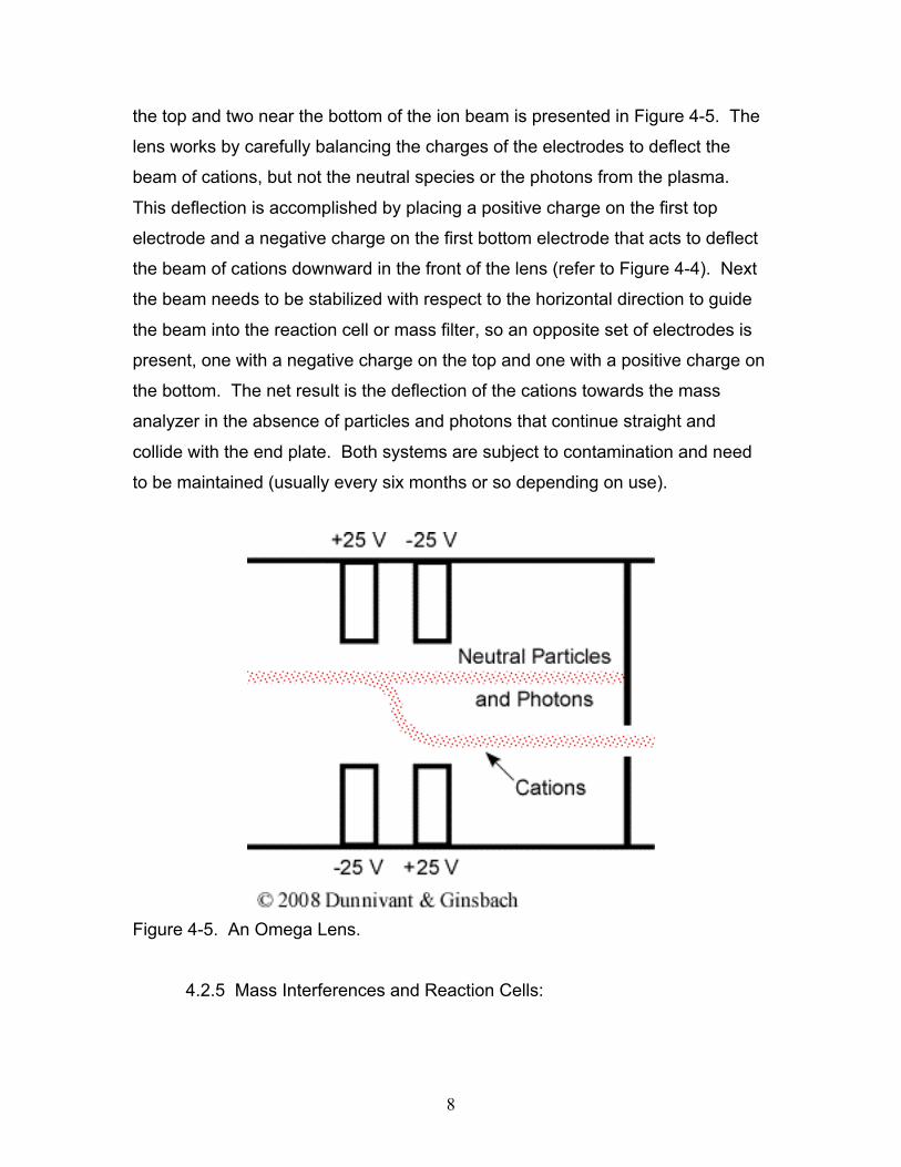
8

the top and two near the bottom of the ion beam is presented in Figure 4-5. The

lens works by carefully balancing the charges of the electrodes to deflect the

beam of cations, but not the neutral species or the photons from the plasma.

This deflection is accomplished by placing a positive charge on the first top

electrode and a negative charge on the first bottom electrode that acts to deflect

the beam of cations downward in the front of the lens (refer to Figure 4-4). Next

the beam needs to be stabilized with respect to the horizontal direction to guide

the beam into the reaction cell or mass filter, so an opposite set of electrodes is

present, one with a negative charge on the top and one with a positive charge on

the bottom. The net result is the deflection of the cations towards the mass

analyzer in the absence of particles and photons that continue straight and

collide with the end plate. Both systems are subject to contamination and need

to be maintained (usually every six months or so depending on use).

Figure 4-5. An Omega Lens.

4.2.5 Mass Interferences and Reaction Cells:

9

ICP-MS instruments separate and detect analytes based on the atoms

mass to charge ratio. Since the plasma in an ICP system is adjusted to maximize

singularly charged species, sample identity is directly related to atomic mass.

While atomic emission spectrometry, ICP-AES, can be relatively free from

spectral interferences (with monochromator systems that produce nm resolutions

to three-decimal places), certain elements have problematic interferences in ICP-

MS analysis due to the limited unit resolution (one amu) of most mass filters

(especially the most common quadrupole mass filters). All ICP systems are

subject to the nebulizer interferences given in the previous chapter. Spectral

interferences are divided into three categories: isobaric, polyatomic, and doubly-

charged species. Isobaric interferences occur in mass analyzers that only have

unit resolution. For example, 40Ar+ will interfere with 40Ca+ and 114Sn+ will

interfere with 114Cd+. High-resolution instruments will resolve more significant

figures of the cation’s mass and will easily distinguish between these elements.

Polyatomic interferences result when molecular species form in the plasma that

have the same mass as the analyte of interest. Their formation can be

dependant on the presence of trace amounts of O2 and N2 in the Ar or sample,

certain salts in the sample, and the energy of the plasma. For example, 40Ca16O+

can overlay with 56Fe+, 40Ar23Na+ with 63Cu+, and 80Ar2+ and 80Ca2

+ with 80Se+.

The final type of interference occurs with doubly charged species. Since mass

analyzers separate atoms based on their mass to charge ratio, 136Ba2+ interferes

with the quantification of 68Zn+ since their mass to charge ratios are identical.

The presence of any of these types of interferences will result in overestimation

of the analyte concentration. Fortunately there are several ways of overcoming

these interferences.

The easiest, but most expensive, way to overcome all three spectral

interferences is to use a high-resolution mass analyzer, but, at a minimum, this

can double to quadruple the cost of an analysis. Most inexpensive alternatives

include the use of interference equations to estimate the concentration of the

interfering element or polyatomic species, the use of a cool plasma technique to

10

minimize the formation of polyatomic interferences, and the use of collision

and/or reaction cells prior to the entry to the mass filter. These three techniques

will be discussed in detail below.

Interference Equations: Most elements are present on the Earth in their

known solar abundance (the isotopic composition of each element that was

created during the formation of our solar system). Important exceptions are

elements in the uranium and thorium decay series, most notably lead. For these

elements, the isotopic ratios are dependent upon the source of the sample. For

example, lead isotope ratios found in the environment can be attributed to at

least three possible sources: geologic lead, leaded gasoline, and mined lead

shot from bullets.

Interference equations are mathematical relationships based on the

known abundances of each element that are used to calculate the total

concentration of all of the isotopes of a particular ion. Isobaric correction is

relatively easy when two or more isotopes of each element (the analyte and the

interfering isotope) are present in the solar abundance. There are two ways to

correct for this type of interference: (1) the analyte of interest can be monitored

at a different mass unit (different isotope), or (2) the interfering element can be

quantified as a different isotope (mass unit) and the result can be subtracted from

the analyte concentration. Polyatomic interferences can be corrected for in the

same manner but to a less effective degree. This type of correction is illustrated

in the following example taken from the ICP-MS primer from Agilent

Technologies Company, a manufacturer of ICP-MS systems.

Example 4.1 Arsenic is an important and common pollutant in

groundwater and an industrial and agricultural pollutant. The analyte of

interest is 75As but 40Ar35Cl has an identical mass on a low-resolution

mass filter system, and since most water samples contain chloride, this

interfering ion will be present in varying concentrations. These can be

11

corrected for by doing the following instrumental and mathematical

analysis. Note that all analysis suggested below require external standard

calibration or for the instrument to be operated in semi-quantitative mode

(a way of estimating analyte concentrations based on the calibration of a

different element or isotope).

1. Acquire data at masses 75, 77, 82, and 83.

2. Assume the signal at mass 83 is form 83Kr and use this to estimate

the signal from 82Kr (based on solar abundances).

3. Subtract the estimated contribution from 82Kr from the signal at 82.

The residual value should be the counts per second for 82Se.

4. Use the estimated 82Se data to predict the size of the signal from 77Se on mass 77 (again, based on solar abundances).

5. Subtract the estimated 77Se contribution from the counts per

second signal at mass 77. The residual value should be from 40Ar37Cl.

6. Use the calculated 40Ar37Cl data to estimate the contribution on

mass 75 from 40Ar35Cl.

7. Subtract the estimated contribution from 40Ar35Cl on mass 75. The

residual is 75As.

This process may seem complicated but is necessary to obtain

accurate concentration data for As in the absence of a high-

resolution mass filter. It should also be noted that this type of

analysis has limitations. (1) If another interference appears at any

of the alternative mass units used, the process will not work. (2) If

the intensity of interference is large, then a large error in the analyte

concentration will result.

Cool Plasma Technique: The ionization of Ar-based polyatomic species in

the normal “hot” plasma can be overcome by operating the radiofrequency at a

12

lower wattage (from 600 to 900 W) and therefore lowering the temperature of the

plasma. This technique, a function on all modern ICP-MS systems, allows for the

removal of polyatomic interferences in the analysis of K, Ca, and Fe. One

downside is the tendency to form more matrix induced oxide cations.

Collision/Reactor Cells: The limitations of the two techniques described

above, and the price of high-resolution mass spectrometry, led to the

development of collision and reaction cells in the late 1990s and early 21th

century to remove these interferences. Numerous Ph.D. dissertations, as well as

research and development programs in industry, are active in this area and there

are books specifically devoted to this topic. Two basic types of approaches have

been used, (1) a collision cell that uses He to select for an optimum kinetic

energy by slowing interfering ions relative to the analyte and only allowing the

passage of the higher energy analyte and (2) reaction cells that promote

reactions between a reagent gas and the interferences in order to remove them

from detection.

The actual collision/reaction cell is a quadru-, hexa- or octa-pole that is

considerable smaller than the subsequent quadrupole (mass filter) and is

enclosed in a chamber that can contain higher pressures then the surrounding

vacuum chamber. No mass separation occurs in the multi-pole since only a DC

current is applied to the poles. Instead, the main purpose of the multi-pole is to

keep the beam focused/contained to provide a space for the necessary collisions

or chemical reactions to occur. While the number of poles in the reaction cell

varies with different instruments, the larger number of poles allows for a more

effective cell since the cross-sectional area of the ion beam is larger for an octa-

pole over a hexa- or quadu-pole. The majority of collision/reaction cells can be

operated in either mode by altering the gas utilized by the system. The price of

the instruments increases slightly with the addition of these cells, however

removing interferences with a collision cell is still less expensive than the

alternative; a high-resolution mass filter.

13

Collision Cells: In a collision cell a non-reactive gas, usually He, is used to

remove polyatomic ions that have the same mass to charge ratio as the analyte

of interest. These multi-pole collisions cells are relatively small as compared to

the mass filtering quadrupole and confine the ion beam from the plasma. Helium

gas is added to the cell while the analyte of interest (an atomic species) and the

interferent (a polyatomic species) move through the chamber. Polyatomic

species are larger then atomic species and therefore collide with the He gas

more often. The net result of these collisions is a greater reduction in the kinetic

energy (measured in eVs) of the polyatomic species in relationship to the atomic

species. As the polyatomic and analyte ions exit the collision cell, they are

screened by a discriminator voltage. A discriminator voltage is the counterpart to

an accelerating lens and contains a slit with a positive voltage; this process is

commonly referred to as kinetic energy discrimination. When a positive voltage

is applied to this gate, only cations possessing sufficient kinetic energy will pass

through the slit. Smaller cations retaining more of their energy, after being

subjected to the collisions with He, will pass through the slit while larger

polyatomic cations that have been slowed by the He collisions will be repelled by

the voltage. The polyatomic species that do not pass into the mass analyzer

collide with the walls of the chamber, are neutralized and removed by the

vacuum system. Common interferences that are removed in this manner are

sample matrix-based interferences such as 35Cl16O+ from interfering with 51V+, 40Ar12C+ from interfering with 52Cr+, 23Na40Ar+ from interfering with 63Cu+, 40Ar35Cl+

from interfering with 75As+, and plasma-based interferences such as 40Ar16O+ and 40Ar38Ar+. Interfering polyatomic species can be reduced down to ppt levels

through kinetic energy discrimination. An animation of a collision cell is shown in

Animation 4.1.

14

Animation 4.1. A Collision Cell.

Reaction Cells: The physical structure and design of a collision cell,

depending on the manufacturer, is similar or identical to that of a reaction cell.

However, instead of utilizing an inert gas such as helium, more reactive gases

are introduced into the cell. H2 is the most common reactive gas but CH4, O2, and

NH3 are also used. Table 4.1 shows a variety of reaction gases and their

intended use.

Table 4.1 Reagent Gases used in Collision and Reaction Cell ICP-MS Systems.

(Source: Koppenaal, et al., 2004, J. Anal. At. Spectrom., 19, 561-570)

Collision Gas

Purpose

He, Ar, Ne, Xe Used as a collision gas to decrease the

kinetic energy of the polyatomic

interference

H2, NH3, Xe, CH4, N2 Used in charge exchange reactions

O2, N2O, NO, CO2 Used to oxidize the interference or

analyte

15

H2, CO Used to reduce the interference

CH4, C2H6, C2H4, CH3F, SF6, CH3OH Used in adduction reactions to remove

interferences

The purpose of the reactive gas is to break up or create chemical species,

through a set of chemical reactions, and change their polyatomic masses to one

that does not coincide with the mass of the analyte of interest. These cells have

significantly extended the elemental range of ICP-MS to include some very

important elements; the most important being 39K+, 40Ca+, and 56Fe+ which had

previously been difficult to measure due to the interferences of 38Ar1H+, 40Ar+, and 40Ar16O+, respectively. The removal of interferences can be divided into three

general categories: charge exchange, atom transfer, and adduct formation (i.e.

condensation reactions).

A generic reaction for a charge transfer reaction would be

A+ + B+ + R A+ + B + R+

where A+ is the analyte, B+ is the isobaric interferent, and R is the reagent gas.

An example of a charge exchange reaction is removal of the cationic Ar dimer in

the analysis of selenium.

80Se+ + 80Ar2

+ + H2 80Se+ + 40Ar40Ar + H2+

The neutral Ar dimer is now removed by the photon stop and vacuum and 80Se+

is easily transported through the mass filter. Another specific case would be the

interference of 40Ar+ with the measurement of 40Ca+. The reaction is

40Ca+ + 40Ar+ + H2 40Ca+ + 40Ar + H2

+

16

In this reaction, the interfering cationic species is neutralized and removed by the

vacuum and does not enter the MS. It should be noted that in charge exchange

reactions, the ionization potential of the reagent gas must lie between the

ionization potentials of the interfering ion and the analytes in order to promote

charge transfer from the interfering ion instead of the analyte. Such a

requirement is not necessary for atom transfer and adduction

formation/condensation reactions. Two such reactions follow.

Atom Addition Reaction

A+ + B+ + R AR+ + B

Fe+ + ArO+ + N2O FeO+ + ArO+ + N2

In this case the interference of ArO+ with the measurement of Fe is removed by

oxidizing the Fe to its oxide that has a different mass from the argon oxide and

quantifying Fe as FeO+.. Another example is given below for the removal of 90Zr

interference in the detection of 90Sr. 90Sr+ + 90Zr+ + 1/2O2 90Sr+ + 90ZrO+

These chemical reactions in the cell create cations that can potentially

interfere with other analytes, hence it is not uncommon for these problematic

analytes to be measured singularly (no multi-elemental analysis). As a result, the

reaction cell mode is frequently utilized for singular applications or for argon

interferences (ex. 40Ar+ and 40Ar 16O+) with hydrogen since the products of the

reaction do not interfere with other analytes of interest. If possible, operating the

collision/reaction cell in the collision mode is preferable since the interferences

are removed from the system. After the spectral interferences have been

removed by either process, the ion beam is separated by mass to charge ratio

with the mass filter. An animation of a typical reaction occurring in a reaction cell

with H2 is shown in Animation 4.2.

17

Animation 4.2. Reaction Cell.

4.2.6 Mass Filters (Mass Analyzers)

Mass analyzers separate the cations based on ion velocity, mass, or mass

to charge ratio. A number of mass filters/analyzers are available. These can be

used individually or coupled in a series of mass analyzers to improve mass

resolution and provide more conclusive analyte identification. This text will only

discuss the most commonly available ones for ICP systems.

The measure of “power” of a mass analyzer is resolution, the ratio of the

average mass (m) of the two adjacent ion peaks being separated to the mass

difference (Δm) of the adjacent peaks, represented by

Rs = m/Δm

Resolution (RS) is achieved when the midpoint between two adjacent peaks is

within 10 percent of the baseline just before and after the peaks of interest (the

valley between the two peaks). Resolution requirements can range from high-

resolution instruments that may require discrimination of a few ten thousands

18

(1/10 000) of a gram molecular weight (0.0002) to low-resolution instruments that

only require unit resolution (28 versus 29 atomic mass units; amu). Resolution

values for commonly available instruments can range from 250 to 500 000.

Before introducing the various types of mass analyzers, remember our

current location of the mass analyzer in the overall ICP-MS system. The sample

has been introduced to the nebulizer, atomized and ionized by the plasma,

accelerated and manipulated by various lenses, sent through a collision/reaction

cell, and finally enters the mass analyzer. Now the packet of cations need to be

separated based on their momentum, kinetic energy, or mass-to-charge ratio

(m/z). Often the terms mass filter and mass analyzer are used interchangeable,

as is done in this Etextbook. But, first a controversy in the literature needed to be

addressed with respect to how a mass filter actually separates ions.

Some resources state that all mass analyzers separate ions with respect

to their mass to charge ratio while others are more specific and contend that only

quadrupoles separate ions by mass to charge ratios. The disagreement in

textbooks lies in what components of the MS are being discussed. If one is

discussing the affect of the accelerator plates and the mass filter, then all mass

filters separate based on mass to charge ratios. This occurs because the charge

of an ion will be a factor that determines the velocity a particle of a given mass

has after interacting with the accelerator plate in the electronic, magnetic sector,

and time of flight mass analyzers. But after the ion has been accelerated, a

magnetic section mass filter actually separates different ions based momentums

and kinetic energies while the time of flight instrument separates different ions

based on ion velocities (arrival times at the detector after traveling a fixed length).

In the other case, no matter what the momentum or velocity of an ion, the

quadrupole mass analyzer separates different ions based solely on mass to

charge ratios (or the ability of the ion to establish a stable path in an oscillating

electrical field). These differences may seem semantic but some users insist on

19

this clarification. For the discussions below, in most cases, mass to charge will

be used for all mass analyzers.

4.2.6.1 Magnetic sector mass filter: It has been known for some time that

the trajectory of point charge, in our case a positively charged ion, can be altered

by an electrical or magnetic field. Thus, the first MS systems employed

permanent magnets or electromagnets to bend the packets of ions in a semi-

circular path and separated ions based on their momentum and kinetic energy.

Common angles of deflection are 60, 90, and 180 degrees. The change in

trajectory of the ions is caused by the external force of the magnetic field. The

magnitude of the centripetal force, which is directly related to the ions velocity,

resists the magnetic field’s force. Since each mass to charge ratio has a distinct

kinetic energy, a given magnetic field strength will separate individual mass to

charge ratios through space. A slit is placed in front of the detector to aid in the

selection of a single mass to charge ratio at a time.

A relatively simple mathematical description will allow for a better

understanding of the magnetic field and the ions centripetal force. First, it is

necessary to compute the kinetic energy (KE) of an ion with mass m possessing

a charge z as it moves through the accelerator plates. This relationship can be

described by

KE = ½ mv2 = zeV

where e is the charge of an electron (1.60 x 10-19 C), v is the ion velocity, and V

is the voltage between the two accelerator plates (shown in the Animation 1.5

below). Fortunately for the ionizations occurring in the plasma, most ions have a

charge of +1. As a result, an ions’ kinetic energy will be inversely proportional to

its mass. The two forces that determine the ions path, the magnetic force (FM)

and the centripetal force (FC), are described by

20

FM = Bzev

and

FC = (mv2)/r

where B is the magnetic field strength and r is the radius of curvature of the

magnetic path. In order for an ion of particular mass and charge to make it to the

detector, the forces FM and FC must be equal. This obtains

BzeV = (mv2)/r

which upon rearrangement yields

v = (Bzer)/m .

Substituting this last equation into our first KE equation yields

m/z = (B2r2e)/2V

Since e (the charge of an electron) is constant and r (the radius of curvature) is

not altered during the run, altering the magnetic field (B) or the voltage between

the accelerator plates (V) will vary the mass to charge ratio that can pass through

the slit and reach the detector. By holding one constant and varying the other

throughout the range of m/z values, the various mass to charge ratios can be

separated. One option is to vary the magnetic field strength while keeping the

voltage on the accelerator plates constant.

In general, it is difficult to quickly vary the magnetic field strength, and

while this is problematic in chromatography it is of little consequence with ICP

instruments. Generally, several complete mass to charge scans are desired for

21

accurate analyte identification and this can be completed ICP analysis by simply

sampling longer. This entire problem can be overcome in modern magnetic

sector instruments by rapidly sweeping the voltage between the accelerator

plates, in order to impart different momentums on the ions, as opposed to

sweeping the field strength. This second mass scanning technique holds the

magnetic field constant while changing the centripetal force placed on the ions by

varying the voltage on the accelerator plates. Due to the operational advantages

of this technique, most electromagnets hold the magnetic field strength (B) and

vary the voltage (V) on the accelerator plates.

The magnetic sector mass filter is illustrated in Animation 4.3 below. As

noted above, although B and r are normally held constant, this modern design is

difficult to animate, so we will illustrate a magnetic sector MS where B, the

magnetic field, is varied to select for different ions. After ions pass the cones at

the ICP MS interface, they are uniformly accelerated by the constant voltage

between the two accelerator plates/slits on the left side of the figure. As the

different ions travel through the electromagnet, the magnetic field is varied to

select for different m/z ratios. Ions with the same momentum or kinetic energy

(and therefore mass) pass through the exit slit together and are measured by the

detector, followed by the next ion, and so on.

Animation 4.3. Illustration of a Magnetic Sector MS.

22

While magnetic sector mass filters were once the only tool used to create

a mass spectrum, they are becoming less common today. This is due to the size

of the instrument and its weight. As a result, many magnetic sector instruments

have been replaced by quadrupole systems that are much smaller, lighter, and

able to perform extremely fast scans. Magnetic sector instruments are still used

in cases where extremely high-resolution is required such as with double-

focusing instruments (discussed later in this section).

4.2.6.2 Quadrupole mass filter: Quadrupole mass filters have become

the most common type of mass filters today due to their relatively small size, light

weight, low cost, and rapid scan times (less than 100 ms). This type of mass

filter is most commonly used in conjunction with ICP systems because they are

able to operate at a relatively high pressure (5 x 10-5 torr) as compared to lower

pressures required in other mass filters. The quadrupole has also gained

widespread use in tandem MS applications (a series of MS analyzers).

Despite the fact that quadrupoles produce the majority of mass spectra

today as mentioned earlier, they are not true mass spectrometers. Actual mass

spectrometers produce a distribution of ions either through time (time of flight

mass spectrometer) or space (magnetic sector mass spectrometer). The

quadrupole’s mass resolving properties are instead a result of the ion’s stability

within the oscillating electrical field.

A quadrupole system consists of four rods that are arranged at an equal

distance from each other in a parallel manner. Paul and Steinwegen theorized in

1953 that hyperbolic cross-sections were necessary. In practice, it has been

found that circular cross sections are both effective and easier to manufacture.

Each rod is less than a cm in diameter and usually less then 15 cm long. Ions

are accelerated by a negative voltage plate before they enter the quadrupole and

23

travel down the center of the rods (in the z direction). However, the ions’

trajectory in the z direction is not altered by the quadrupole’s electric field.

The various ions are separated by applying a time independent dc

potential as well as a time dependent ac potential. The four rods are divided up

into pairs where the diagonal rods have an identical potential. The positive dc

potential is applied to the rods in the X-Z plane and the negative potential is

applied to the rods in the Y-Z plane. The subsequent ac potential is applied to

both pairs of rods but the potential on one pair is the opposite sign of the other or

commonly referred to as being 180˚ out of phase (Figure 4-6).

Mathematically the potential that ions are subjected to are described by

the following equations:

where Φ is the potential applied to the X-Z and Y-Z rods respectively, ω is the

angular frequency (in rad/s) and is equal to 2πv where v is the radio frequency of

the field, U is the dc potential and V is the zero-to-peak amplitude of the radio

frequency voltage (ac potential). The positive and negative signs in the two

equations reflect the change in polarity of the opposing rods (electrodes). The

values of U range from 500 to 2000 volts and V ranges from 0 to 3000 volts.

24

Figure 4-6. AC and DC Potentials in the Quadrupole MS.

25

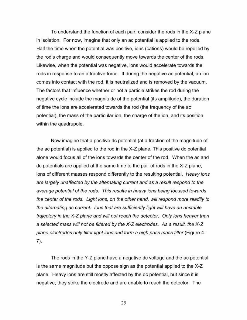
To understand the function of each pair, consider the rods in the X-Z plane

in isolation. For now, imagine that only an ac potential is applied to the rods.

Half the time when the potential was positive, ions (cations) would be repelled by

the rod’s charge and would consequently move towards the center of the rods.

Likewise, when the potential was negative, ions would accelerate towards the

rods in response to an attractive force. If during the negative ac potential, an ion

comes into contact with the rod, it is neutralized and is removed by the vacuum.

The factors that influence whether or not a particle strikes the rod during the

negative cycle include the magnitude of the potential (its amplitude), the duration

of time the ions are accelerated towards the rod (the frequency of the ac

potential), the mass of the particular ion, the charge of the ion, and its position

within the quadrupole.

Now imagine that a positive dc potential (at a fraction of the magnitude of

the ac potential) is applied to the rod in the X-Z plane. This positive dc potential

alone would focus all of the ions towards the center of the rod. When the ac and

dc potentials are applied at the same time to the pair of rods in the X-Z plane,

ions of different masses respond differently to the resulting potential. Heavy ions

are largely unaffected by the alternating current and as a result respond to the

average potential of the rods. This results in heavy ions being focused towards

the center of the rods. Light ions, on the other hand, will respond more readily to

the alternating ac current. Ions that are sufficiently light will have an unstable

trajectory in the X-Z plane and will not reach the detector. Only ions heaver than

a selected mass will not be filtered by the X-Z electrodes. As a result, the X-Z

plane electrodes only filter light ions and form a high pass mass filter (Figure 4-

7).

The rods in the Y-Z plane have a negative dc voltage and the ac potential

is the same magnitude but the oppose sign as the potential applied to the X-Z

plane. Heavy ions are still mostly affected by the dc potential, but since it is

negative, they strike the electrode and are unable to reach the detector. The

26

lighter ions respond to the ac potential and are focused towards the center of the

quadrupole. The ac potential can be thought of as correcting the trajectories of

the lighter ions, preventing them from striking the electrodes in the Y-Z plane.

These electrical parameters result in the construction of a low mass pass filter.

When both the electrodes are combined into the same system, they are

able to selectively allow a single mass to charge ratio to have a stable trajectory

through the quadrupole. Altering the magnitude of the ac and dc potential

changes the mass to charge ratio that has a stable trajectory resulting in the

construction of mass spectra. These ions possess a stable trajectory at different

magnitudes and reach the detector at different times. The graph of the combined

effect, shown in Figure 4-7c, is actually a simplification of the actual stability

diagram.

27

Figure 4-7. A “Conceptual” Stability Diagram

One way to generate an actual stability diagram is to perform a series of

experiments where a single mass ion is introduced into the quadrupole. The dc

28

and ac voltages are allowed to vary and the stability of the ion is mapped. After

performing a great number of experiments the resulting plot would look like

Figure 4-8. The shaded area under the curve represents values of ac and dc

voltages where the ion has a stable trajectory through the potential and would

reach the detector. The white space outside the stability diagram indicates ac

and dc voltages where the ion would not reach the detector.

While any ac and dc voltages that fall inside the stability diagram could be

utilized, in practice, quadrupoles keep the ratio of the dc to ac potential constant,

while the scan is performed by changing the magnitude of the ac and dc

potential. The result of this is illustrated as the mass scan line intersecting the

stability diagram in Figure 4-8. The graphs below the stability diagram

correspond to specific points along the scan and help to illustrate the ions’

trajectories in the X-Z and Y-Z plane (Figure 4-8). While the mass to charge ratio

of the ion remains constant in each pair of horizontal figures, the magnitude of

the applied voltages are changing while their ratio stays constant. As a result,

examining points along the mass scan line in Figure 4-8 is equivalent to shifting

the position of the high and low pass mass filters with respect to the x axis

illustrated in Figure 4-7. Even though the mass is not changing for the stability

diagram discussed here, the mass that has a stable trajectory is altered.

29

Figure 4-8. Stability Diagram for a Single Ion Mass. Used with permission from

the Journal of Chemical Education, Vol. 75, No. 8, 1998, p. 1051; copyright ©

1998, Division of Chemical Education, Inc.

In the above figure, the graph corresponding to point A indicates that the

ion is too light to pass through the X-Z plane because of the high magnitude of

the ac and dc potentials. As a result, its oscillation is unstable, and it eventually

impacts the electrode. The motion of the Y axis is stable because the

combination of the ac potential as well as the negative dc potential causes

30

destructive interference. This is the graphical representation of the ac potential

correcting the trajectory of the light ions in the Y-Z plane. At point B the

magnitude of voltages has been altered so the trajectories of the ion in both the

X-Z and Y-Z plane are stable and the ion successfully reaches the detector. At

point C, the ion has been eliminated by the low mass pass filter. In this case, the

ac potential is too low to allow the ion to pass through the detector and it strikes

the rod. This is caused by the ions increased response to the negative dc

potential in the Y-Z plane. The trajectory in the X-Z axis is stable since the dc

potential focusing the ion towards the center of the poles overwhelms the ac

potential.

Until this point, the stability diagram shown above is only applicable to a

single mass. If a similar experiment were to be performed using a different

mass, the positions of the ac and dc potential on the x and y axes would be

altered but the overall shape of the curve would remain the same. Fortunately,

there is a less time consuming way to generate the general stability diagram for a

quadrupole mass filter. This derivation requires a complex understanding of

differential equations and is beyond the scope of an introductory text, but the

solution can be explained graphically (Figure 4-9). The parameters in the axes

are explained below the figure.

31

Figure 4-9. The General Stability Diagram

While this derivation is particularly complex, the physical interpretation of

the result helps explain how a quadrupole is able to perform a scan. The final

solution is dependent on six variables, but the simplified two-variable problem is

shown in Figure 4-9. Utilizing the reduced parameters, a and q, the problem

becomes a more manageable two-dimensional problem. While the complete

derivation allows researchers to perform scans in multiple ways, this discussion

will focus only on the basic mode that makes up the majority of mass

spectrometers. For the majority of commercially available mass spectrometers,

the magnitude of the ac potential (V) and the dc potential (U) are the only

parameters that are altered during run time. The rest of the parameters that

describe K1 and K2 are held constant. The values for K1 and K2 in the general

stability diagram can be attributed to the following equations:

The parameters that make up K1 and K2 are exactly what we predicted

when listing the variables earlier that would affect the point charge. Both K terms

32

depend upon the charge of the ion e, its position within the quadrupole r, and the

frequency of the ac oscillation ω. These parameters can be altered, but for the

majority of applications remain constant. The charge of the ion (e) can be

assumed to be equivalent to positive one, +1, for almost all cases. The distance

from the center of the quadrupole (r) is carefully controlled by the manufacturing

process and an electronic lens that focuses the ions into the center of the

quadrupole and is also a constant. Also the angular frequency (ω) of the applied

ac waveform can be assumed to be a constant for the purposes of most

spectrometers and for this discussion.

The first important note for the general stability diagram is the relationship

between potential and mass. The general stability diagram (Figure 4-8) is

illustrated where there is an inverse relationship between the two. Figures 4-9

and 4-10 shows the lighter ions (m-1) are higher on the mass scan line and the

heavy ions (m+1) are lower on the line. This is why in Figure 4-8 at point A, the

molecule was too light for the selected frequencies, and it was too heavy at point

C.

From the general stability diagram, it is also possible to explain how an

instrument’s resolution can be altered. The resolution is improved when the

mass scan line intersects the smallest area at the top of the stability diagram

(Figure 4-10). The resolution can be improved when the slope of the mass line is

increased and the slope is directly related to the ratio of U and V. The resolution

will subsequently increase until the line no longer intersects the stability diagram.

While it would be best for the line to intersect at the apex of the stability diagram,

this is impractical due to fluctuations in the ac (V) and dc (U) voltages. As a

result, the line intersects a little below this point allowing the quadrupole to obtain

unit resolution (plus or minus one amu).

Once the resolution has been determined, the ratio of the ac to dc

potential is left unchanged throughout the scan process. To perform a scan, the

33

magnitude of the ac and dc voltages is altered while their ratio remains constant.

This places a different mass inside the stability diagram. For example, if the ac

and dc voltages are doubled, the mass to charge ratio of the selected ion would

also be doubled as illustrated in the second part of Figure 4-10. By scanning

throughout a voltage range, the quadrupole is able to create the majority of mass

spectra produced in today’s chemical laboratories.

34

Figure 4.10 Quadrupole Mass Scan. Used with permission from the Journal of

Chemical Education, Vol. 63, No. 7, 1998, p. 621; copyright © 1986, Division of

Chemical Education, Inc.

35

View Animation 4-4 for an illustration of how the trajectory of ions of different

masses are changed during a mass scan.

Animation 4.4 Illustration of Cations in a Quadrupole Mass Filter.

4.2.6.3 Quadrupole ion trap mass filter: While the operation of the ion trap

was characterized shortly after the linear quadrupole in 1960 by Paul and

Steinwedel, its application in the chemical laboratory was severely limited. This

was due to difficulties associated with manufacturing a circular electrode and

performance problems. These performance problems were overcome when a

group at Finnigan MAT lead by Stafford discovered two breakthroughs that lead

to the production of a commercially available ion trap mass filter. The first ion

trap developed used a mode of operation where a single mass could be stored in

the trap when previously all of the ions had to be stored. Their next important

discovery was the ability for 1 mtorr of helium gas to improve the instruments

resolution. The helium molecules’ collisions with the ions reduced their kinetic

energy and subsequently focused them towards the center of the trap.

After these initial hurdles were cleared, many new techniques were

developed for a diverse set of applications especially in biochemistry. This is a

result of its comparative advantage over the quadrupole when analyzing high

molecular mass compounds (up to 70,000 m/z) to unit resolution in commonly

36

encountered instruments. The ion trap is also an extremely sensitive instrument

that allows a molecular weight to be determined with a small number of

molecules. The ion trap is also the only mass filter that can contain ions that

need to be analyzed for any significant duration of time. This allows the

instrument to be particularly useful in monitoring the kinetics of a given reaction.

The most powerful application of the ion trap is its ability to be used in tandem

mass spectrometry.

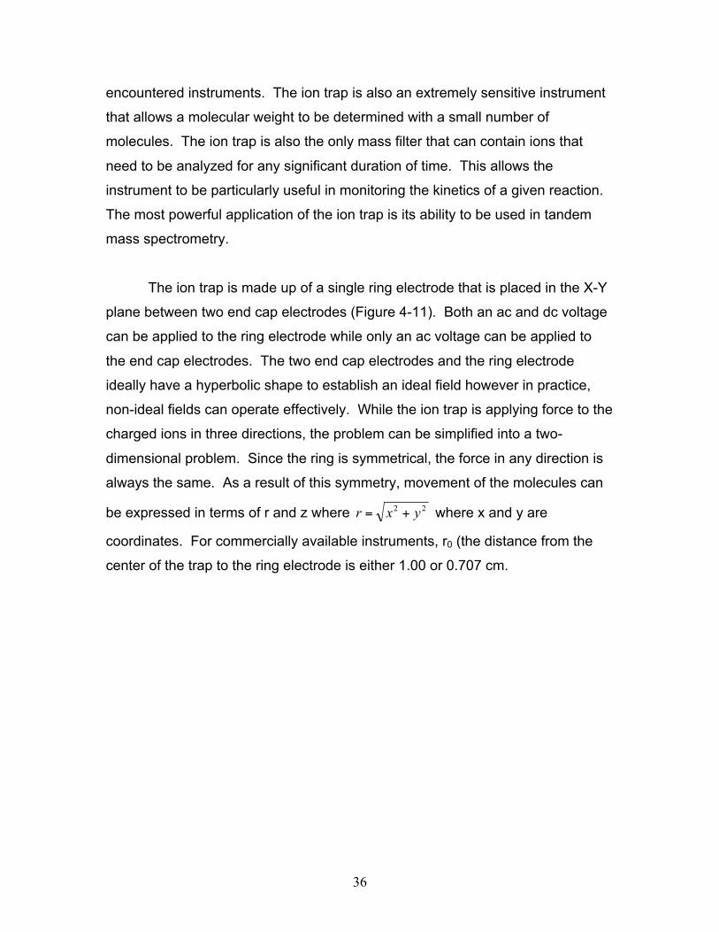
The ion trap is made up of a single ring electrode that is placed in the X-Y

plane between two end cap electrodes (Figure 4-11). Both an ac and dc voltage

can be applied to the ring electrode while only an ac voltage can be applied to

the end cap electrodes. The two end cap electrodes and the ring electrode

ideally have a hyperbolic shape to establish an ideal field however in practice,

non-ideal fields can operate effectively. While the ion trap is applying force to the

charged ions in three directions, the problem can be simplified into a two-

dimensional problem. Since the ring is symmetrical, the force in any direction is

always the same. As a result of this symmetry, movement of the molecules can

be expressed in terms of r and z where where x and y are

coordinates. For commercially available instruments, r0 (the distance from the

center of the trap to the ring electrode is either 1.00 or 0.707 cm.

37

Figure 4-11. A Cross Section of the Ion Trap

After the sample molecules have been ionized by the ionzation source,

they enter into the ion trap through an electric gate located on a single end cap

electrode. This gate functions in the same fashion as the one that is utilized in

time of flight (TOF) mass spectrometry (Section 4.2.6.4). The gate’s purpose is

to prevent a large number of molecules from entering into the trap. If too many

sample molecules enter into the trap, the interaction with other molecules

becomes significant resulting in space-charge effects, a distortion of the electrical

field that minimizes the ion trap’s performance. Once the ions enter the trap,

their collisions with the helium gas focus the ions towards the center of the trap.

An ac frequency is also applied to the ring electrode to assist in focusing the ions

towards the center of the trap.

In the ion trap, the ring electrode oscillates with a very high frequency

(typically 1.1 MHz) while both the end cap electrodes are kept at a ground

potential (U equals 0 Volts). This frequency causes the ions to oscillate in both

38

the r and z direction (Figure 4-12). The oscillation in the r direction is an

expected response to the force generated by the ring electrode. The oscillation

in the z direction, on the other hand, may seem counter intuitive. This is a

response to both the grounded end cap electrodes and the shape of the ring

electrode. When the ac potential increases, the trajectory of the ion becomes

unstable in the z direction. The theoretical basis for this motion will be discussed

later. While it would be convenient to describe the ion trap’s function as a point

charge responding to an electrical field, the complexity of the generated field

makes this impractical.

39

Figure 4-12 The Trajectories of a Single Mass Within the Electrical Field. Figure

6 from Wong and Cooks, 1997. Reprinted with permission of Bioanalytical

Systems, Inc., West Lafayette, IN.

The simplest way to understand how the ion trap creates mass spectra is

to study how ions respond to the electrical field. It is necessary to begin by

constructing a stability diagram for a single ion. Imagine a single mass to charge

ratio being introduced into the ion trap. Then, the ac and dc voltages of the ring

electrode are altered and the ions stability in both the z and r directions are

determined simultaneously. If this experiment was performed multiple times, the

stability diagram for that single mass would look similar to Figure 4-14.

Figure 4-13 A Single Mass Stability Diagram for an Ion Trap. Adapted from

Figure 5 from Wong and Cooks, 1997. Reprinted with permission of Bioanalytical

Systems, Inc., West Lafayette, IN.

40

The yellow area indicates the values of the ac and dc voltages where the

given mass has a stable trajectory in the z direction but the ion’s trajectory in the

r direction is unstable. As a result, the ion strikes the ring electrode, is

neutralized, and removed by the vacuum. The blue area shows the voltages

where the ion has a stable trajectory in the r direction, but not in the z direction.

At these voltages, the ion exits the trap through the slits in the end cap electrode

towards a detector. The detector is on if the analyst is attempting to generate a

mass spectrum, and can be left off if the goal is to isolate a particular mass to

charge ratio of interest. The gray-purple area is where the stability in both the r

and z directions overlap. For these voltages, the ion has a stable trajectory and

remains inside the trap.

Similar to the quadrupole mass filter, differential equations are able to

expand the single mass stability diagram to a general stability diagram. The

derivation of this result requires an in depth understanding of differential

equations, so only the graphical result will be presented here (Figure 4-14). The

solution is simplified from a six-variable problem, similar to the quadrupole

discussion earlier, to a simpler two-variable problem.

41

Figure 4-14 A General Stability Diagram. Adapted from Figure 5 from Wong and

Cooks, 1997. Reprinted with permission of Bioanalytical Systems, Inc., West

Lafayette, IN.

From the general stability diagram it becomes visible how scans can be

performed by just altering the ac voltage on the ring electrode. But before we

discuss the ion trap’s operation it is necessary to understand the parameters that

affect ions stability within the field. The terms K1 and K2 are characterized by the

following equations:

42

As expected, these parameters are very similar to the ones that resulted

from the general stability diagram for the quadrupole mass filter. These

parameters, like in the quadrupole, are also kept constant during a scan. The

charge of the particle (e), the distance from the center of the trap to the ring

electrode (r0), and the radial frequency of the ac voltage (ω) are all kept constant

during the run. While it would be possible to alter both the ac and dc voltages, in

practice it is only necessary to alter the ac voltage (V) of the ring electrode. The

dc voltage (U) on the other hand, is kept at zero. If the dc voltage is kept at a

ground potential, increasing the ac voltage will eventually result in an unstable

trajectory in the z direction. When ac voltage creates a qz value that is greater

than 0.908, the particle will be ejected from the trap towards a detector through

the end cap electrode. As illustrated below, the qz value is dependent on the

mass to charge ratio of the particle, each different mass has a unique ac voltage

that causes them to exit the trap.

For example, let’s place four different ion masses into the ion trap where

each has a single positive charge. The general stability diagram in Figure 4-15 is

identical to Figure 4-14 except that it is focused around a dc voltage (U) of zero

and the scale is enlarged; thus, ax is equal to zero through a scan. A mass scan

is performed by starting the ring electrode out at a low ac voltage. Each distinct

mass has a unique qz value, which is visually illustrated by placing these particles

on the stability diagram (line). As the ac frequency begins to increase, the qz

values for these masses also increases. Once the qz value becomes greater

than 0.908, the ions still have a stable trajectory in the r direction but now have

an unstable trajectory in the z direction. As a result, they are ejected out of the

trap through the end cap electrode towards the detector.

43

Figure 4-15 A Stability Diagram During a Sample Scan

The stability diagram above at A, B, and C was the result of taking a

snapshot of the ac voltage during the scan and placing each mass at its

corresponding qz values for that particular voltage. In this mode of operation, the

lightest masses (m1) are always ejected from the trap (Figure 4-15 B) before the

heaver masses (m2). The heaviest masses (m3 and m4) still remain in the trap at

point C. To eject these ions, a very large ac voltage is necessary. This voltage

is so high that it becomes extremely difficulty to eject ions over a m/z value of

650. Since it is impractical to apply such high voltages to the electrode and its

44

circuits, a new method of operation needed to be discovered so the ion trap

could analyze more massive molecules.

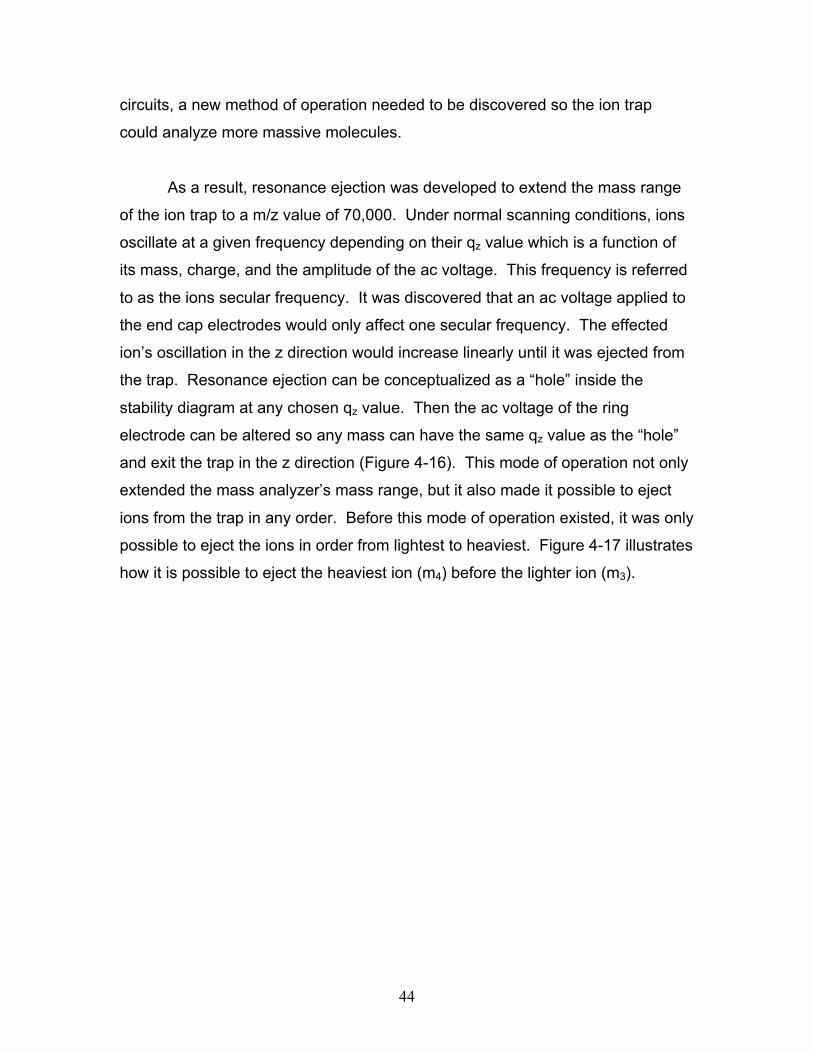
As a result, resonance ejection was developed to extend the mass range

of the ion trap to a m/z value of 70,000. Under normal scanning conditions, ions

oscillate at a given frequency depending on their qz value which is a function of

its mass, charge, and the amplitude of the ac voltage. This frequency is referred

to as the ions secular frequency. It was discovered that an ac voltage applied to

the end cap electrodes would only affect one secular frequency. The effected

ion’s oscillation in the z direction would increase linearly until it was ejected from

the trap. Resonance ejection can be conceptualized as a “hole” inside the

stability diagram at any chosen qz value. Then the ac voltage of the ring

electrode can be altered so any mass can have the same qz value as the “hole”

and exit the trap in the z direction (Figure 4-16). This mode of operation not only

extended the mass analyzer’s mass range, but it also made it possible to eject

ions from the trap in any order. Before this mode of operation existed, it was only

possible to eject the ions in order from lightest to heaviest. Figure 4-17 illustrates

how it is possible to eject the heaviest ion (m4) before the lighter ion (m3).

45

Figure 4-16 A Sample Resonance Ejection Scan

The resonance ejection mode of operation is one reason why the ion trap

is such a valuable tool. It not only greatly extends the mass range of the mass

analyzer, but it also increased its applications in tandem spectroscopy. The

ability to isolate any given mass under 70,000 amu is an extremely powerful tool.

Through the use of both modes of operation, the ion trap has become a valuable

tool in performing many specialized mass separations.

View Animation 4.5 at this time for an illustration of how an ion trap mass

filter contains and ejects ions of given mass to charge ratios.

46

Animation 4.5 Illustration of an Ion Trap Mass Filter.

4.2.6.4 Time-of-Flight (TOF) mass filter: While time-of-flight mass filters

were one of the first modern MS systems to be developed, they had limited use

due to their need for very fast electronics to process the data. Developments in

fast electronics and the need for mass filters capable of resolving high mass

ranges (such as in geological analysis of isotopes) has renewed interest in time

of flight systems.

Entry into the TOF mass filter is considerably different than with other

mass filters. The entry has to be pulsed or intermittent in order to allow for all of

the ions entering the TOF to reach the detector before more ions are created.

With sources that operate in a pulsing fashion such as in ICP or direct insertion

of the sample, the TOF functions easily as a mass analyzer. In sources that

continual produce ions such as an ICP, the use of a TOF is a bit more difficult. In

order to use a TOF system with these continuous sources, an electronic gate

47

must be used to create the necessary pulse of ions. The gate changes the

potential on an accelerator plate to only allow ions to enter the TOF mass filter in

pulses. When the slit has a positive charge, ions will not approach the entryway

to the mass analyzer and are retained in the ionization chamber. When all of the

previously admitted ions have reached the detector, the polarity on the

accelerator(s) is again changed to negative and ions are accelerated toward the

slit(s) and into the TOF mass analyzer. This process is repeated until several

scans of each cation peak has been measured. (This type of ionization and slit

pulsing will be shown in the animation below).

Prior to developing the mathematics behind TOF separations a simple

summary is useful. Mass to charge ratios in the TOF instrument are determined

by measuring the time it takes for ions to pass through the “field-free” drift tube to

the detector. The term “field-free” is used since there is no electronic or

magnetic field affecting the ions. The only force applied to the ions occurs at the

repulsion plate and the acceleration plate(s) where ions obtain a constant kinetic

energy (KE). All of the ions of the same mass to charge ratio entering the TOF

mass analyzers have the same kinetic energy and velocity since they have been

exposed to the same voltage on the plates. Ions with different mass to charge

ratios will have velocities that will vary inversely to their masses. Lighter ions will

have higher velocities and will arrive at the detector earlier than heavier ones.

This is due to the relationship between mass and kinetic energy.

KE = mv2/2

The kinetic energy of an ion with a mass m and a total charge of q = ze is

described by:

mv2/2 = qVS = zeVS

48

where VS is potential difference between the accelerator plates, z is the charge

on the ion, and e is the charge of an electron (1.60 x 10-19 C). The length (d) of

the drift tube is known and fixed, thus the time (t) required to travel this distance

is

t = d/v .

By solving the previous equation for v and substituting it into the above equation

we obtain

.

In a TOF mass analyzer, the terms in parentheses are constant, so the mass to

charge of an ion is directly related to the time of travel. Typical times to traverse

the field-free drift tube are 1 to 30 ms.

Advantages of a TOF mass filter include their simplicity and ruggedness

and a virtually unlimited mass range. However, TOF mass filters suffer from

limited resolution, related to the relatively large distribution in flight times among

identical ions (resulting from the physical width of the plug of ions entering the

mass analyzer).

49

Animation 4.6 illustrations how a pulsed accelerator plate/slit acts as a gate for a

reflectiveTOF mass filter system.

50

Animation 4.6. Illustration of a TOF Mass Filter.

4.2.6.5 Double Focusing Systems: The magnetic sector MS described

earlier is referred to as a single-focusing instrument since it only uses the

magnetic component to separate ion mass to charge ratios. This can be

improved by adding a second electrostatic-field based mass filter, and is referred

to as double focusing. A magnetic field instrument focuses on the distribution of

translational energies imparted on the ions leaving the ionization source as a

means of separation. But in doing so, the magnetic sector instruments broaden

the range of kinetic energies of the ions, resulting in a loss of resolution. If we

combine both separation techniques by passing the ions separately through an

electrostatic (to focus the kinetic energy of the ion packet) and magnetic field (to

focus the translational energies of the ion packet), we will greatly improve our

resolution. In fact, by doing this we can measure ion masses to within a few

parts per million (precision) which results in a resolution of ~2500. Compare this

to the unit resolutions (28 versus 29 Daltons) discussed at the beginning of this

section (under resolution). On the downside, these instruments can be costly.

4.2.6.6 Tandem Mass Spectroscopy: Mass spectroscopy is commonly

referred to as a confirmatory technique since there is little doubt (error) in the

identity of an analyte. To be even more certain of an analyte’s identify, two or

even three, mass spectrometers can be used in series (the output of one MS is

the input of another MS). Subsequent MS systems will select for a specific ion

from the second MS and separate the masses in this peak for further

identification. This technique allows for unit resolution or better in the first MS,

subsequently separating the masses of a given peak in the second and third MS,

and identified based on a three to four decimal place mass. You should be able

to see the confirmatory nature of this technique. Mass filters of choice for use in

tandem include magnetic sector, electrostatic, quadrupole, and ion trap systems.

51

4.2.7 Detectors:

Once the analytes have been ionized, accelerated, and separated in the

mass filter, they must be detected. This is most commonly performed with an

electron multiplier (EM), much like the photoelectron multipliers used in optical

spectroscopy. In MS systems, the electron multiplier is insensitive to ion charge,

ion mass, or chemical nature of the ion (as a photomultiplier is relatively

insensitive to the wavelength of a photon). The EMs in ICP-MS systems are

usually discrete dynodes EMs since these can be easily modified to extend their

dynamic range.

A continuous EMs is typically horn shaped and are made of glass that is

heavily doped with lead oxide. When a potential is placed along the length of the

horn, electrons are ejected as ions strike the surface. Ions usually strike at the

entrance of the horn and the resulting electrons are directed inward (by the

shape of the horn), colliding sequentially with the walls and generating more and

more electrons with each collision. Potentials across the horn can range from

high hundreds of volts to 3000 V. Signal amplifications are in the 10 000 fold

range with nanosecond response times. Animation 4-7 illustrates the response

of a continuous electron multiplier as ions, separated in a mass filter, strike its

surface.

Animation 4.7. Illustration of a Continuous-Dynode Electron Multiplier.

A standard discrete electron multiplier is shown in Animation 4.8 is

actually a connected series of phototubes. In a discrete system each dynode is

held at a +90 V potential as compared to immediately adjacent dynodes. As a

cation hits the first cathode, one or more electrons are ejected and pulled toward

the next cathode. These electrons eject more and more electrons as they go

forward producing tens to hundreds of thousands of electrons and amplifying the

52

signal by a factor of 106 to 108. This allows for extremely low detection limits in

the parts per billion (ppb) to parts per trillion ranges (ppt). Such an EM is shown

in Animation 4.8.

Animation 4.8 Illustration of a Standard Discrete-Dynode Electron Multiplier.

In order to extend the dynamic range of an EM to cover relatively high

analyte concentration (in the ppm range), some manufactures have incorporated

two EM detector in one by including a switch that allows high signals to be

counted in a digital manner in order to prevent the overload of signal, and use

analogue counting to analyze low concentration samples. Such an EM detector

is illustrated in Animation 4.9.

53

Animation 4.9 Illustration of a Dual (Gated ) Discrete-Dynode Electron Multiplier.

Another form of MS detector is the Faraday Cup with counts each ion

entering the detector zone. These detectors are less expensive but provide no

amplification of the signal and are not used in typical instruments due to their

poor detection limits.

One of the latest detectors to reach the market is a microchannel plate, a

form of an array transducer also called an electro-optical ion detector (EOID).

The EOID is a circular disk that contains numerous continuous electron

multipliers (channels). Each channel has a potential applied across it and each

cation reaching the detector will generate typically up to 1000 electrons. The

electrons produce light as they impinge on a phosphorescent screen behind the

disk containing the channels. An optical array detector, using fiber optic

technology, records the flashes of light and produces a two dimensional

resolution of the ions. The advantage of an EOID is their ability to greatly

increase the speed of mass determinations by detecting a limited range of

masses simultaneously, thus reducing the number of discrete magnetic field

adjustments required over a large range of masses. The positioning of the

dispersed beam of cations is easier to visualize for a magnetic sector MS, but the

EOIDs have applications in most mass filter systems. Unfortunately, EOIDs have

not been adapted as rapidly as expected by instrument manufacturers.

4.3 Summary

Mass spectrometry detection greatly expands the applications of ICP

system in the analysis of metals. Not only can more elements be analyzed, as

compared to FAAS, FAES, and ICP-AES, but isotopic data can be collected. A

variety of sample introduction techniques and mass filters make the ICP-MS a

diverse instrument. But increased capabilities and lower detection limits come

54

with a relatively high price tag. For example, a basic ICP-MS costs in the range

of $70-80 thousand while a basic ICP-MS with reaction cell-quadrupole

technology costs around $150 thousand; high-resolution instruments can cost as

high as $600 thousand or more, and some are not even commercially available.

Mass spectrometry is in a constant and rapid state of development. In this

Etextbook, we have focused on the basic mass analyzers, such as the

quadrupole, ion trap, time of flight and magnetic sector (double focusing)

designs. Recent technological advances have allowed for the development of

two upcoming instruments; a new magnetic sector mass analyzer (Walder, et al.,

Journal of Analytical Atomic Spectrometry, 1992, 7, 571-575) and orbital trap

(Makarov, Analytical Chemistry, 2000, 72(6), p.1156). The new magnetic sector

instrument relays on a new sector design referred to as the Mattauch-Herzog

geometry. Although the resolution is relative low (~500) for a high-end

instrument, this mass filter allows for the monitoring of multiple masses at the

exact same time by using a multi-collector-Faraday based detector. The

advantage of this system is that high accuracy in isotopic ratios that can be

obtained. The orbital trap instrument is an electrostatic ion trap capable of

resolution values (Rs) approaching 200 000. While these instruments carry a

high price tag, they greatly increase the normal capabilities of the instrument.

Additional recent breakthroughs in mass spectrometry include the drastic

lowering of detection limits. A new technique referred to as nanostructured

initiator MS (NIMS) is being used in research-grade instruments to measure

biological metabolites. Utilization of these systems with a laser-based systems

produces detection limits are easily at the attomole (10-18) amounts. Specific

molecules in the yoctomole (10-24) levels have even been detected (Nature,

2007, 449, 1003). These systems make the ppb and ppt detection limits

discussed in this Etextbook seem trivial. It is likely that similar detection limits will

soon be achieved for ICP-based instruments.

55

A summary of resolution and price for commercially available instruments

is given in the following table.

Table 4.2 Summary of Mass Filter Features. Source: Personal Communiqué

David Koppenaal, Thermal Scientific & EMSL, Pacific National Laboratory.

Type of Mass Filter Resolution Detection Limit

Approximate Instrument Price

Routine Mass Filters Coupled with ICP

Single Quadrupole

with a collision /

reaction cell (CRC)

250-500 low ppb –

high ppt

$150 000 - $200 000

Ion Trap (no longer

available)

1 000 –

10 000

ppb $400 000 - $500 000

Time of Flight 3000 –

10 000

high ppt $300 000 - $400 000

Double Focusing 10 000 –

20 000

mid to high

ppt

$750 000 - $1 000 000

Fourier Transform 200 000 –

1 000 000

ppb Not commercially available

New Mass Filters

Magnetic Sector /

Multi-collector with

the Mattauch-Herzog

Geometry

~500 high ppb $350 000 - $400 000

Orbital Trap

(Electrostatic Ion

Trap)

150 000 –

200 000

ppb $600 000 (currently only

available with HPLC;

possibly soon to be available

with ICP)