chapter 18 - university of michiganziyang.eecs.umich.edu/~dickrp/sensor-nets/papers/...chapter 18...

Chapter 18

ANALYSIS OF WIRELESS SENSORNETWORKS FOR HABITAT MONITORING

Joseph Polastre1, Robert Szewczyk1, Alan Mainwaring2,David Culler1,2 and John Anderson3

1University of California at BerkeleyComputer Science DepartmentBerkeley, CA 94720{ polastre,szewczyk,culler} @cs.berkeley.edu

2Intel Research Lab, Berkeley2150 Shattuck Ave. Suite 1300Berkeley, CA 94704{ amm,dculler} @intel-research.net

3College of the Atlantic105 Eden StreetBar Harbor, ME [email protected]

Abstract We provide an in-depth study of applying wireless sensor networks (WSNs) toreal-world habitat monitoring. A set of system design requirements were devel-oped that cover the hardware design of the nodes, the sensor network software,protective enclosures, and system architecture to meet the requirements of biol-ogists. In the summer of 2002, 43 nodes were deployed on a small island off thecoast of Maine streaming useful live data onto the web. Although researchersanticipate some challenges arising in real-world deployments of WSNs, manyproblems can only be discovered through experience. We present a set of ex-periences from a four month long deployment on a remote island. We analyzethe environmental and node health data to evaluate system performance. Theclose integration of WSNs with their environment provides environmental dataat densities previously impossible. We show that the sensor data is also usefulfor predicting system operation and network failures. Based on over one million

2 Polastre et. al.

data readings, we analyze the node and network design and develop networkreliability profiles and failure models.

Keywords: Wireless Sensor Networks, Habitat Monitoring, Microclimate Monitoring, Net-work Architecture, Long-Lived Systems

18.1 IntroductionThe emergence of wireless sensor networks has enabled new classes of ap-

plications that benefit a large number of fields. Wireless sensor networks havebeen used for fine-grain distributed control [27], inventory and supply-chainmanagement [25], and environmental and habitat monitoring [22].

Habitat and environmental monitoring represent a class of sensor networkapplications with enormous potential benefits for scientific communities. In-strumenting the environment with numerous networked sensors can enablelong-term data collection at scales and resolutions that are difficult, if notimpossible, to obtain otherwise. A sensor’s intimate connection with its im-mediate physical environment allows each sensor to provide localized mea-surements and detailed information that is hard to obtain through traditionalinstrumentation. The integration of local processing and storage allows sensornodes to perform complex filtering and triggering functions, as well as to applyapplication-specific or sensor-specific aggregation, filtering, and compressionalgorithms. The ability to communicate not only allows sensor data and con-trol information to be communicated across the network of nodes, but nodes tocooperate in performing more complex tasks. Many sensor network servicesare useful for habitat monitoring: localization [4], tracking [7, 18, 20], dataaggregation [13, 19, 21], and, of course, energy-efficient multihop routing [9,17, 32]. Ultimately the data collected needs to be meaningful to disciplinaryscientists, so sensor design [24] and in-the-field calibration systems are cru-cial [5, 31]. Since such applications need to run unattended, diagnostic andmonitoring tools are essential [33].

In order to deploy dense wireless sensor networks capable of recording, stor-ing, and transmitting microhabitat data, a complete system composed of com-munication protocols, sampling mechanisms, and power management must bedeveloped. We let the application drive the system design agenda. Taking thisapproach separates actual problems from potential ones, and relevant issuesfrom irrelevant ones from a biological perspective. The application-driven con-text helps to differentiate problems with simple, concrete solutions from openresearch areas.

Our goal is to develop an effective sensor network architecture for the do-main of monitoring applications, not just one particular instance. Collaborationwith scientists in other fields helps to define the broader application space, as

Analysis of Wireless Sensor Networks for Habitat Monitoring 3

well as specific application requirements, allows field testing of experimentalsystems, and offers objective evaluations of sensor network technologies. Theimpact of sensor networks for habitat and environmental monitoring will bemeasured by their ability to enable new applications and produce new, other-wise unattainable, results.

Few studies have been performed using wireless sensor networks in long-term field applications. During the summer of 2002, we deployed an outdoorhabitat monitoring application that ran unattended for four months. Outdoorapplications present an additional set of challenges not seen in indoor experi-ments. While we made many simplifying assumptions and engineered out theneed for many complex services, we were able to collect a large set of environ-mental and node diagnostic data. Even though the collected data was not highenough quality to make scientific conclusions, the fidelity of the sensor datayields important observations about sensor network behavior. The data anal-ysis discussed in this paper yields many insights applicable to most wirelesssensor deployments. We examine traditional quality of service metrics such aspacket loss; however, the sensor data combined with network metrics providea deeper understanding of failure modes including those caused by the sensornode’s close integration with its environment. We anticipate that with systemevolution comes higher fidelity sensor readings that will give researchers aneven better better understanding of sensor network behavior.

In the following sections, we explain the need for wireless sensor networksfor habitat monitoring in Section 18.2. The network architecture for data flowin a habitat monitoring deployment is presented in Section 18.3. We describethe WSN application in Section 18.4 and analyze the network behaviors de-duced from sensor data on a network and per-node level in Section 18.5. Sec-tion 18.6 contains related work and Section 18.7 concludes.

18.2 Habitat MonitoringMany research groups have proposed using WSNs for habitat and micro-

climate monitoring. Although there are many interesting research problemsin sensor networks, computer scientists must work closely with biologists tocreate a system that produces useful data while leveraging sensor network re-search for robustness and predictable operation. In this section, we examine thebiological need for sensor networks and the requirements that sensor networksmust meet to collect useful data for life scientists.

18.2.1 The Case For Wireless Sensor NetworksLife scientists are interested in attaining data about an environment with

high fidelity. They typically use sensors on probes and instrument as muchof the area of interest as possible; however, densely instrumenting any area

4 Polastre et. al.

is expensive and involves a maze of cables. Examples of areas life scientistscurrently monitor are redwood canopies in forests, vineyard microclimates,climate and occupancy patterns of seabirds, and animal tracking. With theseapplications in mind, we examine the current modes of sensing and introducewireless sensor networks as a new method for obtaining environmental andhabitat data at scales and resolutions that were previously impractical.

Traditional data loggers for habitat monitoring are typically large in sizeand expensive. They require that intrusive probes be placed in the area ofinterest and the corresponding recording and analysis equipment immediatelyadjacent. Life scientists typically use these data loggers since they are commer-cially available, supported, and provide a variety of sensors. Probes includedwith data loggers may create a “shadow effect”–a situation that occurs when anorganism alters its behavioral patterns due to an interference in their space orlifestyle [23]. Instead, biologists argue for the miniaturization of devices thatmay be deployed on the surface, in burrows, or in trees. Since interference issuch a large concern, the sensors must be inconspicuous. They should not dis-rupt the natural processes or behaviors under study [6]. One such data loggeris the Hobo Data Logger [24] from Onset Corporation. Due to size, price, andorganism disturbance, using these systems for fine-grained habitat monitoringis inappropriate.

Other habitat monitoring studies install one or a few sophisticated weatherstations an “insignificant distance” (as much as tens of meters) from the areaof interest. A major concern with this method is that biologists cannot gaugewhether the weather station actually monitors a different microclimate due toits distance from the organism under study [12]. Using these readings, bi-ologists make generalizations through coarse measurements and sparsely de-ployed weather stations. A revolution for biologists would be the ability tomonitor the environment on the scale of the organism, not on the scale of thebiologist [28].

Life scientists are increasingly concerned about the potential impacts of di-rect human interaction in monitoring plants and animals in field studies. Dis-turbance effects are of particular concern in a small island situation where itmay be physically impossible for researchers to avoid impacting an entire pop-ulation. Islands often serve as refugia for species that cannot adapt to the pres-ence of terrestrial mammals. In Maine, biologists have shown that even a 15minute visit to a seabird colony can result in up to 20% mortality among eggsand chicks in a given breeding year [2]. If the disturbance is repeated, theentire colony may abandon their breeding site. On Kent Island, Nova Scotia,researchers found that nesting Leach’s Storm Petrels are likely to abandon theirburrows if disturbed during their first 2 weeks of incubation. Additionally, thehatching success of petrel eggs was reduced by 56% due to investigator distur-


bance compared to a control group that was not disturbed for the duration oftheir breeding cycle [3].

Sensor networks represent a significant advance over traditional, invasivemethods of monitoring. Small nodes can be deployed prior to the sensitiveperiod (e.g.,breeding season for animals, plant dormancy period, or when theground is frozen for botanical studies). WSNs may be deployed on small isletswhere it would be unsafe or unwise to repeatedly attempt field studies. Akey difference between wireless sensor networks and traditional probes or dataloggers is that WSNs permit real-time data access without repeated visits tosensitive habitats. Probes provide real-time data, but require the researcher tobe present on-site, while data in data loggers is not accessible until the loggeris collected at a point in the future.

Deploying sensor networks is a substantially more economical method forconducting long-term studies than traditional, personnel-rich methods. It isalso more economical than installing many large data loggers. Currently, fieldstudies require substantial maintenance in terms of logistics and infrastruc-ture. Since sensors can be deployed and left, the logistics are reduced to initialplacement and occasional servicing. Wireless sensor network may organizethemselves, store data that may be later retrieved, and notify operates that thenetwork needs servicing. Sensor networks may greatly increase access to awider array of study sites that are often limited by concerns about disturbanceor lack easy access for researchers.

18.2.2 Great Duck IslandGreat Duck Island (GDI), located at (44.09N, 68.15W), is a 237 acre island

located 15 km south of Mount Desert Island, Maine. The Nature Conservancy,the State of Maine, and the College of the Atlantic (COA) hold much of the is-land in joint tenancy. Great Duck contains approximately 5000 pairs of Leach’sStorm Petrels, nesting in discrete “patches” within the three major habitat types(spruce forest, meadow, and mixed forest edge) found on the island [1]. COAhas ongoing field research programs on several remote islands with well es-tablished on-site infrastructure and logistical support. Seabird researchers atCOA study the Leach’s Storm Petrel on GDI. They are interested in four majorquestions [26]:

1 What is the usage pattern of nesting burrows over the 24-72 hour cyclewhen one or both members of a breeding pair may alternate incubationduties with feeding at sea?

2 What environmental changes occur inside the burrow and on the surfaceduring the course of the seven month breeding season (April-October)?

6 Polastre et. al.

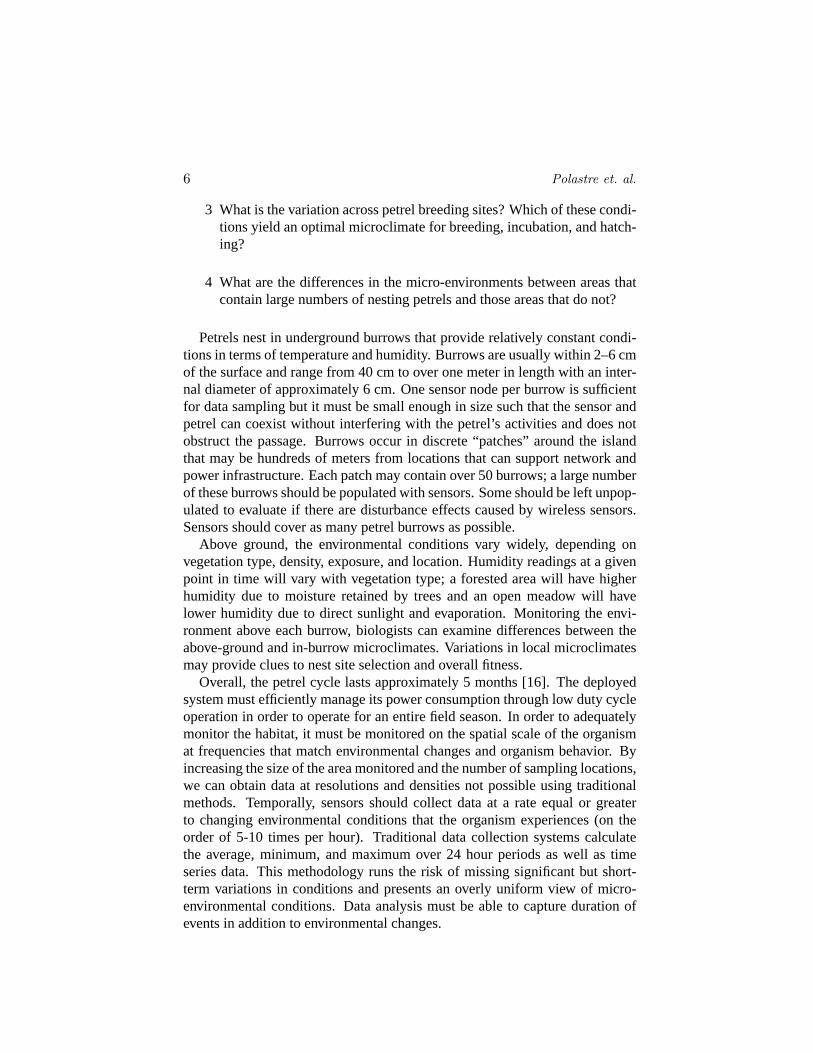
3 What is the variation across petrel breeding sites? Which of these condi-tions yield an optimal microclimate for breeding, incubation, and hatch-ing?

4 What are the differences in the micro-environments between areas thatcontain large numbers of nesting petrels and those areas that do not?

Petrels nest in underground burrows that provide relatively constant condi-tions in terms of temperature and humidity. Burrows are usually within 2–6 cmof the surface and range from 40 cm to over one meter in length with an inter-nal diameter of approximately 6 cm. One sensor node per burrow is sufficientfor data sampling but it must be small enough in size such that the sensor andpetrel can coexist without interfering with the petrel’s activities and does notobstruct the passage. Burrows occur in discrete “patches” around the islandthat may be hundreds of meters from locations that can support network andpower infrastructure. Each patch may contain over 50 burrows; a large numberof these burrows should be populated with sensors. Some should be left unpop-ulated to evaluate if there are disturbance effects caused by wireless sensors.Sensors should cover as many petrel burrows as possible.

Above ground, the environmental conditions vary widely, depending onvegetation type, density, exposure, and location. Humidity readings at a givenpoint in time will vary with vegetation type; a forested area will have higherhumidity due to moisture retained by trees and an open meadow will havelower humidity due to direct sunlight and evaporation. Monitoring the envi-ronment above each burrow, biologists can examine differences between theabove-ground and in-burrow microclimates. Variations in local microclimatesmay provide clues to nest site selection and overall fitness.

Overall, the petrel cycle lasts approximately 5 months [16]. The deployedsystem must efficiently manage its power consumption through low duty cycleoperation in order to operate for an entire field season. In order to adequatelymonitor the habitat, it must be monitored on the spatial scale of the organismat frequencies that match environmental changes and organism behavior. Byincreasing the size of the area monitored and the number of sampling locations,we can obtain data at resolutions and densities not possible using traditionalmethods. Temporally, sensors should collect data at a rate equal or greaterto changing environmental conditions that the organism experiences (on theorder of 5-10 times per hour). Traditional data collection systems calculatethe average, minimum, and maximum over 24 hour periods as well as timeseries data. This methodology runs the risk of missing significant but short-term variations in conditions and presents an overly uniform view of micro-environmental conditions. Data analysis must be able to capture duration ofevents in addition to environmental changes.


It is unlikely that any one parameter or sensor reading could determine whypetrels choose a specific nesting site. Predictive models will require multiplemeasurements of many variables or sensors. These models can then be usedto determine which conditions seabirds prefer. To link organism behavior withenvironmental conditions, sensors may monitor micro-environmental condi-tions (temperature, humidity, pressure, and light levels) and burrow occupancy(by detecting infrared radiation) [22].

Finally, sensor networks should be run alongside traditional methods to val-idate and build confidence in the data. The sensors should operate reliably andpredictably.

18.3 Network ArchitectureIn order to deploy a network that satisfies the requirements of Section 18.2,

we developed a system architecture for habitat monitoring applications. Here,we describe the architecture, the functionality of individual components, andthe interoperability between components.

The system architecture for habitat monitoring applications is a tiered ar-chitecture. Samples originate at the lowest level that consists ofsensor nodes.These nodes perform general purpose computing and networking in addition toapplication-specific sensing. Sensor nodes will typically be deployed in densesensor patchesthat are widely separated. Each patch encompasses a particulargeographic region of interest. The sensor nodes transmit their data through thesensor patch to the sensor networkgateway. The gateway is responsible fortransmitting sensor data from thesensor patchthrough a local transit networkto the remotebase stationthat provides WAN connectivity and data logging.The base station connects to database replicas across the Internet. Finally, thedata is displayed to scientists through any number of user interfaces. Mobiledevices may interact with any of the networks–whether it is used in the fieldor across the world connected to a database replica. The full architecture isdepicted in Figure 18.1.

Sensor nodes are small, battery-powered devices are placed in areas of in-terest. Each sensor node collects environmental data about its immediate sur-roundings. The sensor node computational module is a programmable unit thatprovides computation, storage, and bidirectional communication with othernodes in the system. It interfaces with analog and digital sensors on the sensormodule, performs basic signal processing (e.g.,simple translations based oncalibration data or threshold filters), and dispatches the data according to theapplication’s needs. Compared with traditional data logging systems, it offerstwo major advantages: it cancommunicatewith the rest of the system in realtime and can beretaskedin the field. WSNs may coordinate to deliver data andbe reprogrammed with new functionality.

8 Polastre et. al.

Transit Network

Basestation

Gateway

Sensor Patch

Patch Network

Base-Remote Link

Data Service

Internet

Client Data Browsingand Processing

Sensor Node

Figure 18.1. System architecture for habitat monitoring

Individual sensor nodes communicate and coordinate with one another inthe same geographic region. These nodes make up asensor patch. The sensorpatches are typically small in size (tens of meters in diameter); in our applica-tion they correspond to petrel nesting patches.

Using a multi-tiered network is particularly advantageous since each habi-tat involves monitoring several particularly interesting areas, each with its owndedicated sensor patch. Each sensor patch is equipped with agateway. Thegateway provides a bridge that connects the sensor network to the base stationthrough a transit network. Since each gateway may include more infrastructure(e.g.,solar panels, energy harvesting, and large capacity batteries), it enablesdeployment of small devices with low capacity batteries. By relying on thegateway, sensor nodes may extend their lifetime through extremely low dutycycles. In addition to providing connectivity to the base station, the gatewaymay coordinate the activity within the sensor patch or provide additional com-putation and storage. In our application, a single repeater node served as thetransit network gateway. It retransmitted messages to the base station using ahigh gain Yagi antenna over a 350 meter link. The repeater node ran at a 100%duty cycle powered by a solar cell and rechargeable battery.


Ultimately, data from each sensor needs to be propagated to the Internet.The propagated data may be raw, filtered, or processed. Bringing direct widearea connectivity to each sensor patch is not feasible–the equipment is toocostly, it requires too much power and the installation of all required equipmentis quite intrusive to the habitat. Instead, the wide area connectivity is broughtto abase station, where adequate power and housing for the equipment is pro-vided. The base station communicates with the sensor patches using the transitnetwork. To provide data to remote end-users, thebase stationincludes widearea network (WAN) connectivity and persistent data storage for the collectionof sensor patches. Since many habitats of interest are quite remote, we choseto use a two-way satellite connection to connect to the Internet.

Data reporting in our architecture may occur both spatially and temporally.In order to meet the network lifetime requirements, nodes may operate in aphased manner. Nodes primarily sleep; periodically, they wake, sample, per-form necessary calculations, and send readings through the network Data maytravel spatially through various routes in the sensor patch, transit network, orwide area network; it is then routed over long distances to the wide area infras-tructure.

Users interact with the sensor network data in two ways. Remote users ac-cess the replica of the base station database (in the degenerate case they interactwith the database directly). This approach allows for easy integration with dataanalysis and mining tools, while masking the potential wide area disconnec-tions with the base stations. Remote control of the network is also providedthrough the database interface. Although this control interface is is sufficientfor remote users, on-site users may often require a more direct interaction withthe network. Small, PDA-sized devices enables such interaction. The datastore replicates content across the WAN and its efficiency is integral to livedata streams and large analyses.

18.4 Application ImplementationIn the summer of 2002, we deployed a 43 node sensor network for habi-

tat monitoring on Great Duck Island. Implementation and deployment of anexperimental wireless sensor network platform requires engineering the ap-plication software, hardware, and electromechanical design. We anticipatedcontingencies and feasible remedies for the electromechanical, system, andnetworking issues in the design of the application that are discussed in thissection.

18.4.1 Application SoftwareOur approach was to simplify the system design wherever possible, to mini-

mize engineering and development efforts, to leverage existing sensor network

10 Polastre et. al.

Figure 18.2 Mica mote(left) with Mica WeatherBoard sensor board for habitatmonitoring includes sensorsfor light, temperature, hu-midity, pressure, and infraredradiation.

platforms and components, and to use off-the-shelf products where appropri-ate to focus attention upon the sensor network itself. We chose to use theMica mote developed by UC Berkeley [14] running the TinyOS operating sys-tem [15].

In order to evaluate a long term deployment of a wireless sensor network,we installed each node with a simple periodic application that meets the bi-ologists requirements defined in Section 18.2. Every 70 seconds, each nodesampled each of its sensors and transmitted the data in a single 36 byte datapacket. Packets were timestamped with 32-bit sequence numbers kept in flashmemory. All motes with sensor boards were transmit-only devices that pe-riodically sampled their sensors, transmitted their readings, and entered theirlowest-power state for 70 seconds. We relied on the underlying carrier senseMAC layer protocol in TinyOS to prevent against packet collisions.

18.4.2 Sensor board designTo monitor petrel burrows below ground and the microclimate above the

burrow, we designed a specialized sensor board called the Mica Weather Board.Environmental conditions are measured with a photoresistive sensor, digitaltemperature sensor, capacitive humidity sensor, and digital pressure sensor. Tomonitor burrow occupancy, we chose a passive infrared detector (thermopile)because of its low power requirements. Since it is passive, it does not inter-fere with the burrow environment. Although a variety of surface mount andprobe-based sensors were available, we decided to use surface mount compo-nents because they were smaller and operated at lower voltages. Although aprobe-based approach has the potential to allow precise co-location of a sensorwith its phenomenon, the probes typically operated at higher voltages and cur-rents than equivalent surface mount parts. Probes are more invasive since theypuncture the walls of a burrow. We designed and deployed a sensor board withall of the sensors integrated into a single package. A single package permittedminiaturization of the node to fit in the size-constrained petrel burrow.


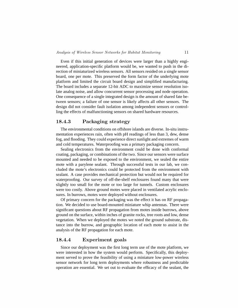
Even if this initial generation of devices were larger than a highly engi-neered, application-specific platform would be, we wanted to push in the di-rection of miniaturized wireless sensors. All sensors resided on a single sensorboard, one per mote. This preserved the form factor of the underlying moteplatform and limited the circuit board design and simplified manufacturing.The board includes a separate 12-bit ADC to maximize sensor resolution iso-late analog noise, and allow concurrent sensor processing and node operation.One consequence of a single integrated design is the amount of shared fate be-tween sensors; a failure of one sensor is likely affects all other sensors. Thedesign did not consider fault isolation among independent sensors or control-ling the effects of malfunctioning sensors on shared hardware resources.

18.4.3 Packaging strategyThe environmental conditions on offshore islands are diverse. In-situ instru-

mentation experiences rain, often with pH readings of less than 3, dew, densefog, and flooding. They could experience direct sunlight and extremes of warmand cold temperatures. Waterproofing was a primary packaging concern.

Sealing electronics from the environment could be done with conformalcoating, packaging, or combinations of the two. Since our sensors were surfacemounted and needed to be exposed to the environment, we sealed the entiremote with a parylene sealant. Through successful tests in our lab, we con-cluded the mote’s electronics could be protected from the environment withsealant. A case provides mechanical protection but would not be required forwaterproofing. Our survey of off-the-shelf enclosures found many that wereslightly too small for the mote or too large for tunnels. Custom enclosureswere too costly. Above ground motes were placed in ventilated acrylic enclo-sures. In burrows, motes were deployed without enclosures.

Of primary concern for the packaging was the effect it has on RF propaga-tion. We decided to use board-mounted miniature whip antennas. There weresignificant questions about RF propagation from motes inside burrows, aboveground on the surface, within inches of granite rocks, tree roots and low, densevegetation. When we deployed the motes we noted the ground substrate, dis-tance into the burrow, and geographic location of each mote to assist in theanalysis of the RF propagation for each mote.

18.4.4 Experiment goalsSince our deployment was the first long term use of the mote platform, we

were interested in how the system would perform. Specifically, this deploy-ment served to prove the feasibility of using a miniature low-power wirelesssensor network for long term deployments where robustness and predictableoperation are essential. We set out to evaluate the efficacy of the sealant, the

12 Polastre et. al.

Figure 18.3. Acrylic enclosures used at different outdoor applications.

radio performance in and out of burrows, the usefulness of the data for biolo-gists including the occupancy detector, and the system and network longevity.Since each hardware and software component was relatively simple, our goalwas to draw significant conclusions about the behavior of wireless sensor net-works from the resulting data.

After 123 days of the experiment, we logged over 1.1 million readings. Dur-ing this period, we noticed abnormal operation among the node population.Some nodes produced sensor readings out of their operating range, others haderratic packet delivery, and some failed. We sought to understand why theseevents had occurred. By evaluating these abnormalities, future applicationsmay be designed to isolate problems and provide notifications or perform self-healing. The next section analyzes node operation and identifies the causes ofabnormal behavior.

18.5 System AnalysisBefore the disciplinary scientists perform the analysis of the sensor data, we

need convincing evidence that the sensor network is functioning correctly. Welook at the performance of the network as a whole in Section 18.5.1 as well asthe failures experienced by individual nodes in Section 18.5.2.

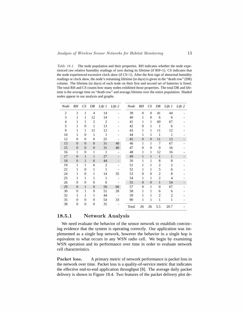
In order to look more closely at the network and node operation, we wouldlike to introduce you to the node community that operated on Great Duck Is-land. Shown in Table 18.1, each of the nodes is presented with their node IDand lifetime in days. Some of the nodes had their batteries replaced and ran fora second “life”. Of importance is that some of the nodes fell victim to raw hu-midity readings of zero or significant clock skew. The number of days after thefirst sign of either abnormality is referred to as the amount of time on “deathrow”. We discuss individual nodes highlighted in Table 18.1 throughout ouranalysis in this section and explain their behavior.


Table 18.1. The node population and their properties. RH indicates whether the node expe-rienced raw relative humidity readings of zero during its lifetime (if RH=1). CS indicates thatthe node experienced excessive clock skew (if CS=1). After the first sign of abnormal humidityreadings or clock skew, the node’s remaining lifetime (in days) is given in the “death row” (DR)column. The lifetime (in days) of each node on their first and second set of batteries is listed.The total RH and CS counts how many nodes exhibited those properties. The total DR and life-time is the average time on “death row” and average lifetime over the entire population. Shadednodes appear in our analysis and graphs.

Node RH CS DR Life 1 Life 2

2 1 1 4 14 -3 1 1 12 14 -4 1 1 2 2 -5 1 0 1 13 -9 1 1 12 12 -10 1 0 1 1 -12 0 0 0 25 -13 0 0 0 31 4015 0 0 0 31 4016 1 0 1 1 -17 0 1 1 27 -18 0 1 6 44 -19 1 1 6 2 -22 1 0 1 1 -24 1 0 1 14 3525 1 1 1 1 -26 0 0 6 6 -29 0 1 0 56 6630 0 1 0 51 2832 1 1 1 44 -35 0 0 0 54 3338 0 0 0 35 -

Node RH CS DR Life 1 Life 2

39 0 0 41 44 -40 1 0 6 6 -41 1 1 60 67 -42 0 1 1 6 -43 1 1 11 12 -44 1 1 1 1 -45 0 0 11 13 -46 1 1 7 67 -47 0 0 0 16 -48 1 1 12 16 -49 1 1 1 1 -50 1 1 8 8 -51 1 1 2 2 -52 1 1 5 6 -53 0 0 2 8 -54 1 1 2 4 -55 0 0 1 54 -57 0 1 0 67 -58 1 1 6 6 -59 1 1 2 2 -90 1 1 1 1 -

Total 26 26 5.5 20.7 -

18.5.1 Network AnalysisWe need evaluate the behavior of the sensor network to establish convinc-

ing evidence that the system is operating correctly. Our application was im-plemented as a single hop network, however the behavior in a single hop isequivalent to what occurs in any WSN radio cell. We begin by examiningWSN operation and its performance over time in order to evaluate networkcell characteristics.

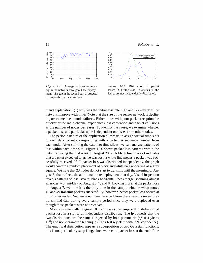
Packet loss. A primary metric of network performance is packet loss inthe network over time. Packet loss is a quality-of-service metric that indicatesthe effective end-to-end application throughput [8]. The average daily packetdelivery is shown in Figure 18.4. Two features of the packet delivery plot de-

14 Polastre et. al.

Jul Aug Sep Oct Nov Dec0

102030405060708090

100

Mea

n pa

cket

del

iver

y ra

te (%

)

Figure 18.4. Average daily packet deliv-ery in the network throughout the deploy-ment. The gap in the second part of Augustcorresponds to a database crash.

0 5 10 15 20 250

0.020.040.060.08

0.10.120.140.160.18

0.2

Missing packets per time slot

Actual packet lossI.I.D. packet loss

Figure 18.5. Distribution of packetlosses in a time slot. Statistically, thelosses are not independently distributed.

mand explanation: (1) why was the initial loss rate high and (2) why does thenetwork improve with time? Note that the size of the sensor network is declin-ing over time due to node failures. Either motes with poor packet reception diequicker or the radio channel experiences less contention and packet collisionsas the number of nodes decreases. To identify the cause, we examine whethera packet loss at a particular node is dependent on losses from other nodes.

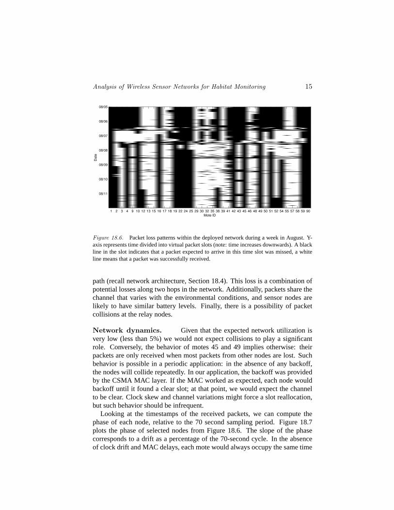
The periodic nature of the application allows us to assign virtual time slotsto each data packet corresponding with a particular sequence number fromeach node. After splitting the data into time slices, we can analyze patterns ofloss within each time slot. Figure 18.6 shows packet loss patterns within thenetwork during the first week of August 2002. A black line in a slot indicatesthat a packet expected to arrive was lost, a white line means a packet was suc-cessfully received. If all packet loss was distributed independently, the graphwould contain a random placement of black and white bars appearing as a graysquare. We note that 23 nodes do not start to transmit until the morning of Au-gust 6; that reflects the additional mote deployment that day. Visual inspectionreveals patterns of loss: several black horizontal lines emerge, spanning almostall nodes,e.g.,midday on August 6, 7, and 8. Looking closer at the packet losson August 7, we note it is the only time in the sample window when motes45 and 49 transmit packets successfully; however, heavy packet loss occurs atmost other nodes. Sequence numbers received from these sensors reveal theytransmitted data during every sample period since they were deployed eventhough those packets were not received.

More systematically, Figure 18.5 compares the empirical distribution ofpacket loss in a slot to an independent distribution. The hypothesis that thetwo distributions are the same is rejected by both parametric (χ2 test yields108) and non-parametric techniques (rank test rejects it with 99% confidence).The empirical distribution appears a superposition of two Gaussian functions:this is not particularly surprising, since we record packet loss at the end of the


Mote ID

Dat

e

1 2 3 4 9 10 12 13 15 16 17 18 19 22 24 25 29 30 32 35 38 39 41 42 43 45 46 48 49 50 51 52 54 55 57 58 59 90

08/05

08/06

08/07

08/08

08/09

08/10

08/11

Figure 18.6. Packet loss patterns within the deployed network during a week in August. Y-axis represents time divided into virtual packet slots (note: time increases downwards). A blackline in the slot indicates that a packet expected to arrive in this time slot was missed, a whiteline means that a packet was successfully received.

path (recall network architecture, Section 18.4). This loss is a combination ofpotential losses along two hops in the network. Additionally, packets share thechannel that varies with the environmental conditions, and sensor nodes arelikely to have similar battery levels. Finally, there is a possibility of packetcollisions at the relay nodes.

Network dynamics. Given that the expected network utilization isvery low (less than 5%) we would not expect collisions to play a significantrole. Conversely, the behavior of motes 45 and 49 implies otherwise: theirpackets are only received when most packets from other nodes are lost. Suchbehavior is possible in a periodic application: in the absence of any backoff,the nodes will collide repeatedly. In our application, the backoff was providedby the CSMA MAC layer. If the MAC worked as expected, each node wouldbackoff until it found a clear slot; at that point, we would expect the channelto be clear. Clock skew and channel variations might force a slot reallocation,but such behavior should be infrequent.

Looking at the timestamps of the received packets, we can compute thephase of each node, relative to the 70 second sampling period. Figure 18.7plots the phase of selected nodes from Figure 18.6. The slope of the phasecorresponds to a drift as a percentage of the 70-second cycle. In the absenceof clock drift and MAC delays, each mote would always occupy the same time

16 Polastre et. al.

08/06 08/07 08/08 08/09 08/10 08/11 08/120

10

20

30

40

50

60

70

Time (days)

Pha

se (s

econ

ds)

13151718494555

13 55

18

15 17

49

45

09:00 12:00 15:000

10

20

30

40

50

60

70

Time (hours)

Pha

se (s

econ

ds)

13151718494555

17

15

55

18

13

49

45

Figure 18.7. Packet phase as a function of time; the right figure shows the detail of the regionbetween the lines in the left figure.

slot cycle and would appear as a horizontal line in the graph. A 5 ppm oscillatordrift would result in gently sloped lines, advancing or retreating by 1 secondevery 2.3 days. In this representation, the potential for collisions exists only atthe intersections of the lines.

Several nodes display the expected characteristics: motes 13, 18, and 55hold their phase fairly constant for different periods, ranging from a few hoursto a few days. Other nodes,e.g.,15 and 17 appear to delay the phase, losing70 seconds every 2 days. The delay can come only from the MAC layer; onaverage they lose 28 msec, which corresponds to a single packet MAC backoff.We hypothesize that this is a result of the RF automatic gain control circuits:in the RF silence of the island, the node may adjust the gain such that it detectsradio noise and interprets it as a packet. Correcting this problem may be doneby incorporating a signal strength meter into the MAC that uses a combina-tion of digital radio output and analog signal strength. This additional backoffseems to capture otherwise stable nodes:e.g.,mote 55 on August 9 transmitsin a fixed phase until it comes close to the phase of 15 and 17. At that point,mote 55 starts backing off before every transmission. This may be caused byimplicit synchronization between nodes caused by the transit network.

We note that potential for collisions does exist: the phases of different nodesdo cross on several occasions. When the phases collide, the nodes back off asexpected,e.g.,mote 55 on August 9 backs off to allow 17 to transmit. Nextwe turn to motes 45 and 49 from Figure 18.6. Mote 45 can collide with motes13 and 15; collisions with other nodes, on the other hand, seem impossible. Incontrast, mote 49, does not display any potential for collisions; instead it showsa very rapid phase change. Such behavior can be explained either though aclock drift, or through the misinterpretation of the carrier sense (e.g.,a motedetermines it needs to wait a few seconds to acquire a channel). We associatesuch behavior with faulty nodes, and return to it in Section 18.5.2.


18.5.2 Node AnalysisNodes in outdoor WSNs are exposed to closely monitor and sense their en-

vironment. Their performance and reliability depend on a number of environ-mental factors. Fortunately, the nodes have a local knowledge of these factors,and they may exploit that knowledge to adjust their operation. Appropriatenotifications from the system would allow the end user to pro-actively fix theWSN. Ideally, the network could request proactive maintenance, or self-heal.We examine the link between sensor and node performance. Although the par-ticular analysis is specific to this deployment, we believe that other systemswill be benefit from similar analyses: identifying outliers or loss of expectedsensing patterns, across time, space or sensing modality. Additionally, sincebattery state is an important part of a node’s self-monitoring capability [33],we also examine battery voltage readings to analyze the performance of ourpower management implementation.

Sensor analysis. The suite of sensors on each node provided analoglight, humidity, digital temperature, pressure, and passive infrared readings.The sensor board used a separate 12-bit ADC to maximize the resolution andminimize analog noise. We examine the readings from each sensor.

Light readings. The light sensor used for this application was a photore-sistor that we had significant experience with in the past. It served as a con-fidence building tool and ADC test. In an outdoor setting during the day, thelight value saturated at the maximum ADC value, and at night the values werezero. Knowing the saturation characteristics, not much work was invested incharacterizing its response to known intensities of light. The simplicity of thissensor combined with ana priori knowledge of the expected response provideda valuable baseline for establishing the proper functioning of the sensor board.As expected, the sensors deployed above ground showed periodic patterns ofday and night and burrows showed near to total darkness. Figure 18.8 showslight and temperature readings and average light and temperature readings dur-ing the experiment.

The light sensor operated most reliably of the sensors. The only behavioridentifiable as failure was disappearance of diurnal patterns replaced by highvalue readings. Such behavior is observed in 7 nodes out of 43, and in 6 casesit is accompanied by anomalous readings from other sensors, such as a 0oCtemperature or analog humidity values of zero.

Temperature readings. A Maxim 6633 digital temperature sensor pro-vided the temperature measurements While the sensor’s resolution is 0.0625oC,in our deployment it only provided a 2oC resolution: the hardware alwayssupplied readings with the low-order bits zeroed out. The enclosure was IR

18 Polastre et. al.

07/21 07/22 07/23 07/24 07/25 07/26 07/27 07/28 07/29

0

10

20

30

40

50

60

70

80

90

100Light Level (%)Temperature (oC)

07/21 07/22 07/23 07/24 07/25 07/26

0

10

20

30

40

50

60

70

80

90


Jul Aug Sep Oct Nov Dec

0

10

20

30

40

50

60

70

80

90


Figure 18.8. Light and temperature time series from the network. From left: outside, inside,and daily average outside burrows.

transparent to assist the thermopile sensor; consequently, the IR radiation fromdirect sunlight would enter the enclosure and heat up the mote. As a result,temperatures measured inside the enclosures were significantly higher than theambient temperatures measured by traditional weather stations. On cloudydays the temperature readings corresponded closely with the data from nearbyweather buoys operated by NOAA.

Even though motes were coated with parylene, sensor elements were leftexposed to the environment to preserve their sensing ability. In the case ofthe temperature sensor, a layer of parylene was permissible. Nevertheless thesensor failed when it came in direct contact with water. The failure manifesteditself in a persistent reading of 0oC. Of 43 nodes, 22 recorded a faulty tem-perature reading and 14 of those recorded their first bad reading during stormson August 6. The failure of temperature sensor is highly correlated with thefailure of the humidity sensor: of 22 failure events, in two cases the humiditysensor failed first and in two cases the temperature sensor failed first. In re-maining 18 cases, the two sensors failed simultaneously. In all but two cases,the sensor did not recover.

Humidity readings. The relative humidity sensor was a capacitive sen-sor: its capacitance was proportional to the humidity. In the packaging process,the sensor needed to be exposed; it was masked out during the parylene seal-ing process, and we relied on the enclosure to provide adequate air circulationwhile keeping the sensor dry. Our measurements have shown up to 15% errorin the interchangeability of this sensor across sensor boards. Tests in a con-trolled environment have shown the sensor produces readings with 5% varia-tion due to analog noise. Prior to deployment, we did not perform individualcalibration; instead we applied the reference conversion function to convert thereadings into SI units.

In the field, the protection afforded by our enclosure proved to be inade-quate. When wet, the sensor would create a low-resistance path between thepower supply terminals. Such behavior would manifest itself in either abnor-


08/05 08/06 08/07 08/08 08/09 08/10 08/110

100

200H

umid

ity (%

)

08/05 08/06 08/07 08/08 08/09 08/10 08/110

2

Vol

tage

(V)

08/05 08/06 08/07 08/08 08/09 08/10 08/110

50

Pac

kets

rece

ived

per h

our

17182955

17182955

17182955

Node 18: extended down−time,followed by self−recovery

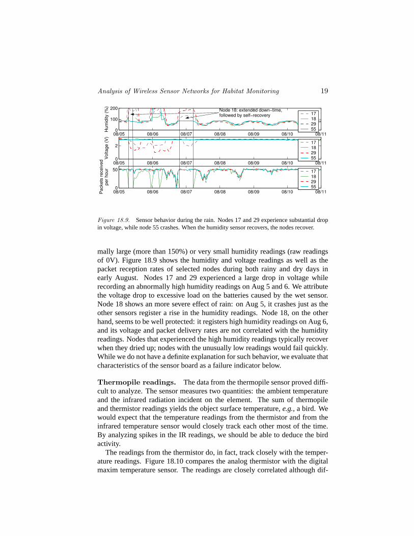
Figure 18.9. Sensor behavior during the rain. Nodes 17 and 29 experience substantial dropin voltage, while node 55 crashes. When the humidity sensor recovers, the nodes recover.

mally large (more than 150%) or very small humidity readings (raw readingsof 0V). Figure 18.9 shows the humidity and voltage readings as well as thepacket reception rates of selected nodes during both rainy and dry days inearly August. Nodes 17 and 29 experienced a large drop in voltage whilerecording an abnormally high humidity readings on Aug 5 and 6. We attributethe voltage drop to excessive load on the batteries caused by the wet sensor.Node 18 shows an more severe effect of rain: on Aug 5, it crashes just as theother sensors register a rise in the humidity readings. Node 18, on the otherhand, seems to be well protected: it registers high humidity readings on Aug 6,and its voltage and packet delivery rates are not correlated with the humidityreadings. Nodes that experienced the high humidity readings typically recoverwhen they dried up; nodes with the unusually low readings would fail quickly.While we do not have a definite explanation for such behavior, we evaluate thatcharacteristics of the sensor board as a failure indicator below.

Thermopile readings. The data from the thermopile sensor proved diffi-cult to analyze. The sensor measures two quantities: the ambient temperatureand the infrared radiation incident on the element. The sum of thermopileand thermistor readings yields the object surface temperature,e.g.,a bird. Wewould expect that the temperature readings from the thermistor and from theinfrared temperature sensor would closely track each other most of the time.By analyzing spikes in the IR readings, we should be able to deduce the birdactivity.

The readings from the thermistor do, in fact, track closely with the temper-ature readings. Figure 18.10 compares the analog thermistor with the digitalmaxim temperature sensor. The readings are closely correlated although dif-

20 Polastre et. al.

07/21 07/22 07/23 07/24 07/25 07/26 07/27 07/28 07/2910

12

14

16

18

Tem

pera

ture

(o C)

07/21 07/22 07/23 07/24 07/25 07/26 07/27 07/28 07/29−28−26−24−22−20−18

Unc

orre

cted

The

rmis

tor (

o C)

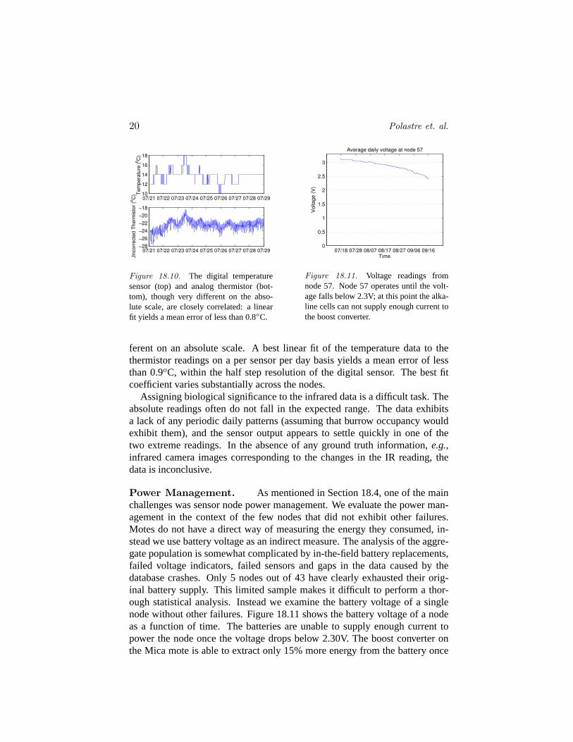
Figure 18.10. The digital temperaturesensor (top) and analog thermistor (bot-tom), though very different on the abso-lute scale, are closely correlated: a linearfit yields a mean error of less than 0.8oC.

07/18 07/28 08/07 08/17 08/27 09/06 09/160

0.5

1

1.5

2

2.5

3

Average daily voltage at node 57

Time

Vol

tage

(V)

Figure 18.11. Voltage readings fromnode 57. Node 57 operates until the volt-age falls below 2.3V; at this point the alka-line cells can not supply enough current tothe boost converter.

ferent on an absolute scale. A best linear fit of the temperature data to thethermistor readings on a per sensor per day basis yields a mean error of lessthan 0.9oC, within the half step resolution of the digital sensor. The best fitcoefficient varies substantially across the nodes.

Assigning biological significance to the infrared data is a difficult task. Theabsolute readings often do not fall in the expected range. The data exhibitsa lack of any periodic daily patterns (assuming that burrow occupancy wouldexhibit them), and the sensor output appears to settle quickly in one of thetwo extreme readings. In the absence of any ground truth information,e.g.,infrared camera images corresponding to the changes in the IR reading, thedata is inconclusive.

Power Management. As mentioned in Section 18.4, one of the mainchallenges was sensor node power management. We evaluate the power man-agement in the context of the few nodes that did not exhibit other failures.Motes do not have a direct way of measuring the energy they consumed, in-stead we use battery voltage as an indirect measure. The analysis of the aggre-gate population is somewhat complicated by in-the-field battery replacements,failed voltage indicators, failed sensors and gaps in the data caused by thedatabase crashes. Only 5 nodes out of 43 have clearly exhausted their orig-inal battery supply. This limited sample makes it difficult to perform a thor-ough statistical analysis. Instead we examine the battery voltage of a singlenode without other failures. Figure 18.11 shows the battery voltage of a nodeas a function of time. The batteries are unable to supply enough current topower the node once the voltage drops below 2.30V. The boost converter onthe Mica mote is able to extract only 15% more energy from the battery once


the voltage drops below 2.5V (the lowest operating voltage for the platformwithout the voltage regulation). This fell far short of our expectations of be-ing able to drain the batteries down to 1.6V, which represents an extra 40%of energy stored in a cell [10]. The periodic, constant power load presentedto the batteries is ill suited to extract the maximum capacity. For this class ofdevices, a better solution would use batteries with stable voltage,e.g.,some ofthe lithium-based chemistries. We advocate future platforms eliminate the useof a boost converter.

Node failure indicators. In the course of data analysis we haveidentified a number of anomalous behaviors: erroneous sensor readings andapplication phase skew. The humidity sensor seemed to be a good indicator ofnode health. It exhibited 2 kinds of erroneous behaviors: very high and verylow readings. The high humidity spikes, even though they drained the mote’sbatteries, correlated with recoverable mote crashes. The humidity readingscorresponding to a raw voltage of 0V correlated with permanent mote outage:55% of the nodes with excessively low humidity readings failed within twodays. In the course of packet phase analysis we noted some motes with slowerthan usual clocks. This behavior also correlates well with the node failure:52% of nodes with such behavior fail within two days.

These behaviors have a very low false positive detection rate: only a singlenode exhibiting the low humidity and two nodes exhibiting clock skew (out of43) exhausted their battery supply instead of failing prematurely. Figure 18.12compares the longevity of motes that have exhibited either the clock skew ora faulty humidity sensor against the survival curve of mote population as awhole. We note that 50% of motes with these behaviors become inoperablewithin 4 days.

18.6 Related WorkAs described in Section 18.2, traditional data loggers are typically large

and expensive or use intrusive probes. Other habitat monitoring studies installweather stations an “insignificant distance” from the area of interest and makecoarse generalizations about the environment. Instead, biologists argue for theminiaturization of devices that may be deployed on the surface, in burrows, orin trees.

Habitat monitoring for WSNs has been studied by a variety of other re-search groups. Cerpa et. al. [7] propose a multi-tiered architecture for habitatmonitoring. The architecture focuses primarily on wildlife tracking instead ofhabitat monitoring. A PC104 hardware platform was used for the implementa-tion with future work involving porting the software to motes. Experimentationusing a hybrid PC104 and mote network has been done to analyze acoustic sig-nals [30], but no long term results or reliability data has been published. Wang

22 Polastre et. al.

0 10 20 30 40 50 60 700

0.1

0.2

0.3

0.4

0.5

0.6

0.7

0.8

0.9

1

Time (days)

Pro

babi

lity

of fa

ilure

Relative humidityClock skewCombinationTotal population

Figure 18.12. Cumulative probability of node failure in the presence of clock skew andanomalous humidity readings compared with the entire population of nodes.

et. al. [29] implement a method to acoustically identify animals using a hybridiPaq and mote network.

ZebraNet [18] is a wireless sensor network design for monitoring and track-ing wildlife. ZebraNet uses nodes significantly larger and heavier than motes.The architecture is designed for an always mobile, multi-hop wireless network.In many respects, this design does not fit with monitoring the Leach’s StormPetrel at static positions (burrows). ZebraNet, at the time of this writing, hasnot yet had a full long-term deployment so there is currently no thorough anal-ysis of the reliability of their sensor network algorithms and design.

The number of deployed wireless sensor network systems is extremely low.There is very little data about long term behavior of sensor networks, let alonewireless networks used for habitat monitoring. The Center for Embedded Net-work Sensing (CENS) has deployed their Extensible Sensing System [11] atthe James Mountain Reserve in California. Their architecture is similar to ourswith a variety of sensor patches connected via a transit network that is tiered.Intel Research has recently deployed a network to monitor Redwood canopiesin Northern California and a second network to monitor vineyards in Oregon.Additionally, we have deployed a second generation multihop habitat monitor-ing network on Great Duck Island, ME. As of this writing, these systems arestill in their infancy and data is not yet available for analysis.

18.7 ConclusionWe have presented the need for wireless sensor networks for habitat mon-

itoring, the network architecture for realizing the application, and the sensornetwork application implementation. We have shown that much care must betaken when deploying a wireless sensor network for prolonged outdoor oper-


ation keeping in mind the sensors, packaging, network infrastructure, appli-cation software. We have analyzed environmental data from one of the firstoutdoor deployments of WSNs. While the deployment exhibited very highnode failure rates and failed to produce meaningful data for the disciplinarysciences, it yielded valuable insight into WSN operation that could not havebeen obtained in simulation or in an indoor deployment. We have identifiedsensor features that predict a 50% node failure within 4 days. We analyzed theapplication-level data to show complex behaviors in low levels of the system,such as MAC-layer synchronization of nodes.

Sensor networks do not exist in isolation from their environment; they areembedded within it and greatly affected by it. This work shows that the anoma-lies in sensor readings can be used to predict node failures with high confi-dence. Prediction enables pro-active maintenance and node self-maintenance.This insight will be very important in the development of self-organizing andself-healing WSNs.

NotesData from the wireless sensor network deployment on Great Duck Island

can be view graphically athttp://www.greatduckisland.net . Ourwebsite also includes the raw data for researchers in both computer scienceand the biological sciences to download and analyze.

This work was supported by the Intel Research Laboratory at Berkeley,DARPA grant F33615-01-C1895 (Network Embedded Systems Technology“NEST”), the National Science Foundation, and the Center for InformationTechnology Research in the Interest of Society (CITRIS).

References

[1] Julia Ambagis. Census and monitoring techniques for Leach’s StormPetrel (Oceanodroma leucorhoa). Master’s thesis, College of the Atlantic,Bar Harbor, ME, USA, 2002.

[2] John G. T. Anderson. Pilot survey of mid-coast maine seabird colonies:An evaluation of techniques. InReport to the State of Maine Departmentof Inland Fisheries and Wildlife, Bangor, ME, USA, 1995.

[3] Alexis L. Blackmer, Joshua T. Ackerman, and Gabrielle A. Nevitta. Ef-fects of investigator disturbance on hatching success and nest-site fidelityin a long-lived seabird, Leach’s Storm-Petrel.Biological Conservation,2003.

[4] Nirupama Bulusu, Vladimir Bychkovskiy, Deborah Estrin, and John Hei-demann. Scalable, ad hoc deployable, RF-based localization. InPro-

24 Polastre et. al.

ceedings of the Grace Hopper Conference on Celebration of Women inComputing, Vancouver, Canada, October 2002.

[5] Vladimir Bychkovskiy, Seapahn Megerian, Deborah Estrin, and MiodragPotkonjak. Colibration: A collaborative approach to in-place sensor cal-ibration. In Proceedings of the 2nd International Workshop on Infor-mation Processing in Sensor Networks (IPSN’03), Palo Alto, CA, USA,April 2003.

[6] Karen Carney and William Sydeman. A review of human disturbanceeffects on nesting colonial waterbirds.Waterbirds, 22:68–79, 1999.

[7] Alberto Cerpa, Jeremy Elson, Deborah Estrin, Lewis Girod, MichaelHamilton, and Jerry Zhao. Habitat monitoring: Application driver forwireless communications technology. In2001 ACM SIGCOMM Work-shop on Data Communications in Latin America and the Caribbean, SanJose, Costa Rica, April 2001.

[8] Dan Chalmers and Morris Sloman. A survey of Quality of Service inmobile computing environments.IEEE Communications Surveys, 2(2),1992.

[9] Benjie Chen, Kyle Jamieson, Hari Balakrishnan, and Robert Morris.Span: An energy-efficient coordination algorithm for topology mainte-nance in ad hoc wireless networks. InProceedings of the 7th AnnualInternational Conference on Mobile Computing and Networking, pages85–96, Rome, Italy, July 2001. ACM Press.

[10] Eveready Battery Company. Energizer no. x91 datasheet.http://data.energizer.com/datasheets/library/primary/alkaline/energizer_e2/x91.pdf .

[11] Michael Hamilton, Michael Allen, Deborah Estrin, John Rottenberry,Phil Rundel, Mani Srivastava, and Stefan Soatto. Extensible sensingsystem: An advanced network design for microclimate sensing.http://www.cens.ucla.edu , June 2003.

[12] David C.D. Happold. The subalpine climate at smiggin holes, KosciuskoNational Park, Australia, and its influence on the biology of small mam-mals.Arctic & Alpine Research, 30:241–251, 1998.

[13] Tian He, Brian Blum, John Stankovic, and Tarek Abdelzaher. AIDA:Adaptive Application Independant Data Aggregation in Wireless SensorNetworks.ACM Transactions in Embedded Computing Systems (TECS),Special issue on Dynamically Adaptable Embedded Systems, 2003.

[14] Jason Hill and David Culler. Mica: a wireless platform for deeply em-bedded networks.IEEE Micro, 22(6):12–24, November/December 2002.

[15] Jason Hill, Robert Szewczyk, Alec Woo, Seth Hollar, David Culler, andKristofer Pister. System architecture directions for networked sensors.


In Proceedings of the 9th International Conference on Architectural Sup-port for Programming Languages and Operating Systems (ASPLOS-IX),pages 93–104, Cambridge, MA, USA, November 2000. ACM Press.

[16] Chuck Huntington, Ron Butler, and Robert Mauck.Leach’s Storm Petrel(Oceanodroma leucorhoa), volume 233 ofBirds of North America. TheAcademy of Natural Sciences, Philadelphia and the American Orinthol-ogist’s Union, Washington D.C., 1996.

[17] Chalermek Intanagonwiwat, Ramesh Govindan, and Deborah Estrin. Di-rected diffusion: a scalable and robust communication paradigm for sen-sor networks. InProceedings of the 6th Annual International Conferenceon Mobile Computing and Networking, pages 56–67, Boston, MA, USA,August 2000. ACM Press.

[18] Philo Juang, Hidekazu Oki, Yong Wang, Margaret Martonosi, Li-ShiuanPeh, and Daniel Rubenstein. Energy-efficient computing for wildlifetracking: Design tradeoffs and early experiences with ZebraNet. InPro-ceedings of the 10th International Conference on Architectural Supportfor Programming Languages and Operating Systems (ASPLOS-X), pages96–107, San Jose, CA, USA, October 2002. ACM Press.

[19] Bhaskar Krishanamachari, Deborah Estrin, and Stephen Wicker. The im-pact of data aggregation in wireless sensor networks. InProceedingsof International Workshop of Distributed Event Based Systems (DEBS),Vienna, Austria, July 2002.

[20] Jie Liu, Patrick Cheung, Leonidas Guibas, and Feng Zhao. A dual-space approach to tracking and sensor management in wireless sensornetworks. InProceedings of the 1st ACM International Workshop onWireless Sensor Networks and Applications, pages 131–139, Atlanta,GA, USA, September 2002. ACM Press.

[21] Samuel Madden, Michael Franklin, Joseph Hellerstein, and Wei Hong.TAG: a Tiny AGgregation service for ad-hoc sensor networks. InPro-ceedings of the 5th USENIX Symposium on Operating Systems Designand Implementation (OSDI ’02), Boston, MA, USA, December 2002.

[22] Alan Mainwaring, Joseph Polastre, Robert Szewczyk, David Culler, andJohn Anderson. Wireless sensor networks for habitat monitoring. InProceedings of the 1st ACM International Workshop on Wireless SensorNetworks and Applications, pages 88–97, Atlanta, GA, USA, September2002. ACM Press.

[23] Ian Nisbet. Disturbance, habituation, and management of waterbirdcolonies.Waterbirds, 23:312–332, 2000.

[24] Onset Computer Corporation. HOBO weather station.http://www.onsetcomp.com .

26 Polastre et. al.

[25] Kris Pister, Barbara Hohlt, Jaein Jeong, Lance Doherty, and J.P. Vainio.Ivy: A sensor network infrastructure for the University of Califor-nia, Berkeley College of Engineering.http://www-bsac.eecs.berkeley.edu/projects/ivy/ , March 2003.

[26] Joseph Polastre. Design and implementation of wireless sensor networksfor habitat monitoring. Master’s thesis, University of California at Berke-ley, Berkeley, CA, USA, 2003.

[27] Bruno Sinopoli, Cory Sharp, Luca Schenato, Shawn Schaffert, andShankar Sastry. Distributed control applications within sensor networks.Proceedings of the IEEE, 91(8):1235–1246, August 2003.

[28] Marco Toapanta, Joe Funderburk, and Dan Chellemi. Development ofFrankliniella species (Thysanoptera: Thripidae) in relation to microcli-matic temperatures in vetch.Journal of Entomological Science, 36:426–437, 2001.

[29] Hanbiao Wang, Jeremy Elson, Lewis Girod, Deborah Estrin, and KungYao. Target classification and localization in habitat monitoring. InPro-ceedings of IEEE International Conference on Acoustics, Speech, andSignal Processing (ICASSP 2003), Hong Kong, China, April 2003.

[30] Hanbiao Wang, Deborah Estrin, and Lewis Girod. Preprocessing in atiered sensor network for habitat monitoring.EURASIP JASP SpecialIssue on Sensor Networks, 2003(4):392–401, March 2003.

[31] Kamin Whitehouse and David Culler. Calibration as parameter estima-tion in sensor networks. InProceedings of the 1st ACM InternationalWorkshop on Wireless Sensor Networks and Applications, pages 59–67,Atlanta, GA, USA, September 2002. ACM Press.

[32] Ya Xu, John Heidemann, and Deborah Estrin. Geography-informed en-ergy conservation for ad hoc routing. InProceedings of the 7th AnnualInternational Conference on Mobile Computing and Networking, pages70–84, Rome, Italy, July 2001. ACM Press.

[33] Jerry Zhao, Ramesh Govindan, and Deborah Estrin. Computing aggre-gates for monitoring wireless sensor networks. InProceedings of the 1stIEEE International Workshop on Sensor Network Protocols and Applica-tions, Anchorage, AK, USA, May 2003.

chapter 18 - university of michiganziyang.eecs.umich.edu/~dickrp/sensor-nets/papers/...chapter 18...

Documents