chapter 13 aimee's work 2003 instructor's edition
TRANSCRIPT

CHAPTER THIRTEEN
STATISTICS
Exercise Set 13.1 1. Statistics is the art and science of gathering, analyzing, and making inferences (predictions) from numerical information obtained in an experiment. 2. Descriptive statistics is concerned with the collection, organization, and analysis of data. Inferential statistics is concerned with making generalizations or predictions from the data collected. 3. Answers will vary. 4. Answers will vary. 5. Insurance companies, sports, airlines, stock market, medical profession 6. Probability is used to compute the chance of occurrence of a particular event when all possible outcomes are known.
Statistics is used to draw conclusions about possible outcomes through observations of only a few particular events. 7. a) A population consists of all items or people of interest. b) A sample is a subset of the population. 8. a) A systematic sample is a sample obtained by selecting every nth item on a list or production line. b) Use a random number table to select the first item, then select every nth item after that. 9. a) A random sample is a sample drawn in such a way that each item in the population has an equal chance of being selected. b) Number each item in the population. Write each number on a piece of paper and put each numbered piece of paper
in a hat. Select pieces of paper from the hat and use the numbered items selected as your sample. 10. a) A cluster sample is a random selection of groups of units. b) Divide a geographic area into sections. Randomly select sections or clusters. Either each member of the selected
cluster is included in the sample or a random sample of the members of each selected cluster is used. 11. a) A stratified sample is one that includes items from each part (or strata) of the population. b) First identify the strata you are interested in. Then select a random sample from each strata. 12. a) A convenience sample uses data that is easily or readily obtained. b) For example, select the first 20 students entering a classroom. 13. a) An unbiased sample is one that is a small replica of the entire population with regard to income, education, gender, race, religion, political affiliation, age, etc. 14. a) No, the method used to obtain the sample is biased. In classes where students are seated alphabetically, brothers
and sisters could be selected from different classes. b) The mean will be greater. Families with many children are more likely to be selected.
15. Stratified sample 16. Systematic sample 17. Cluster sample 18. Random sample 19. Systematic sample 20. Stratified sample 21. Convenience sample 22. Cluster sample 23. Random sample 24. Convenience sample
25. a) – c) Answers will vary. 26. Biased because the subscribers of Consumer Reports are not necessarily representative of the entire population.
27. President; four out of 42 U.S. presidents have been assassinated (Lincoln, Garfield, McKinley, Kennedy). 28. Answers will vary.
407

408 CHAPTER 13 Statistics
Exercise Set 13.2 1. Answers will vary. 2. Yes, the sum of its parts is 142%. The sum of the parts of a circle graph should be 100%. When the total percent of
responses is more than 100%, a circle graph is not an appropriate graph to display the data. A bar graph is more appropriate in this situation.
3. There may have been more car thefts in Baltimore, Maryland than Reno, Nevada because many more people live in Baltimore than in Reno. But, Reno may have more car thefts per capita than Baltimore.
4. Mama Mia’s may have more empty spaces and more cars in the parking lot than Shanghi’s due to a larger parking lot or because more people may walk to Mama Mia’s than to Shanghi’s. 5. Although the cookies are fat free, they still contain calories. Eating many of them may still cause you to gain weight.
6. The fact that Morgan's is the largest department store does not imply it is inexpensive. 7. More people drive on Saturday evening. Thus, one might expect more accidents. 8. Most driving is done close to home. Thus, one might expect more accidents close to home. 9. People with asthma may move to Arizona because of its climate. Therefore, more people with asthma may live in Arizona.
10. We don’t know how many of each professor’s students were surveyed. Perhaps more of Professor Malone’s students than Professor Wagner’s students were surveyed. Also, because more students prefer a teacher does not mean that he or she is a better teacher. For example, a particular teacher may be an easier grader and that may be why that teacher is preferred. 11. Although milk is less expensive at Star Food Markets than at Price Chopper Food Markets, other items may be more expensive at Star Food Markets.
12. Just because they are the most expensive does not mean they will last the longest. 13. There may be deep sections in the pond, so it may not be safe to go wading.
14. Men may drive more miles than women and men may drive in worse driving conditions (like snow). 15. Half the students in a population are expected to be below average.
16. Not all students who apply to a college will attend that college.
17. a)
Percent of National Expenditures Spent on Hospital Care
0
5
10
15
20
25
30
35
40
45
'85 '90 '95 '97 '98 '99 '00
Year
Per
cent

SECTION 13.2 409
17. b)
18. a)
18. b)
19. a)
U.S. Infant Mortality Rate per 1000 Births
0.01.02.03.04.05.06.07.08.0
1994 1995 1996 1997 1998 1999 2000
Year
Per
cent
U.S. Infant Mortality Rate per 1000 Births
6.97.07.17.27.37.47.57.67.77.87.98.0
1994 1995 1996 1997 1998 1999 2000
Year
Per
cent
Median Age at First Marriage for Males
0
5
10
15
20
25
30
1970 1980 1990 2000
Year
Age
Percent of National Expenditures Spent on Hospital Care
31323334353637383940
'85 '90 '95 '97 '98 '99 '00
Year
Per
cent

410 CHAPTER 13 Statistics
19. b)
20. a)
20. b)
21. a) b) Yes. The new graph gives the impression that the percents are closer together.
Median Age at First Marriage for Males
22
23
24
25
26
27
1970 1980 1990 2000
Year
Age
Median Age at First Marriage for Females
0
5
10
15
20
25
1970 1980 1990 2000
Year
Age
Median Age at First Marriage for Females
20
21
22
23
24
25
1970 1980 1990 2000
Year
Age
Percent of Survey Respondents That Purchased Clothing Accessories Online,
Nov. 2000 - Jan. 2001
5.2
4.4
0.0 1.0 2.0 3.0 4.0 5.0 6.0
Female
Male
Percent

SECTION 13.3 411
22. a) 000,000,275
000,000,119
000,000,275
000,000,275000,000,394 =−
%3.432743.0 ≈= increase
b) Radius 1
in. 0.25 in.4
= =
( ) 196349541.00625.025.0 22 ==== πππ rA
20.196 in.≈
c) Radius 3
in. 0.375 in.8
= =
( ) 441786467.0140625.0375.0 22 ==== πππ rA
20.442 in.≈
d) 0.442 0.196 0.246
1.2551020410.196 0.196
− = =
125.5% increase≈
e) Yes, the percent increase in the size of the area from the first circle to the second is greater than the percent increase in population.
23. A decimal point
Exercise Set 13.3
1. A frequency distribution is a listing of observed values and the corresponding frequency of
occurrence of each value.
2. Subtract a lower class limit from the next lower class limit or subtract an upper class limit from the next upper class limit.
3. a) 7 b) 16-22 c) 16 d) 22
4. a) 9 b) 21-29 c) 21 d) 29
5. The modal class is the class with the greatest frequency.
6. The class mark is another name for the midpoint of a class. Add the lower and upper class limits
and divide the sum by 2.
7. a) Number of observations = sum of frequencies = 18 b) Width = 16 9 7− =
c) 16 22 38
192 2
+ = =
d) The modal class is the class with the greatest frequency. Thus, the modal class is 16 - 22. e) Since the class widths are 7, the next class would be 51 - 57. 8. a) Number of observations = sum of frequencies = 25 b) Width = 50 - 40 = 10
c) 5.542
109
2
5950 ==+
d) 40 - 49 and 80 - 89 both contain 7 pieces of data. Thus, they are both modal classes. e) Since the class widths are 10, the next class would be 100 – 109.
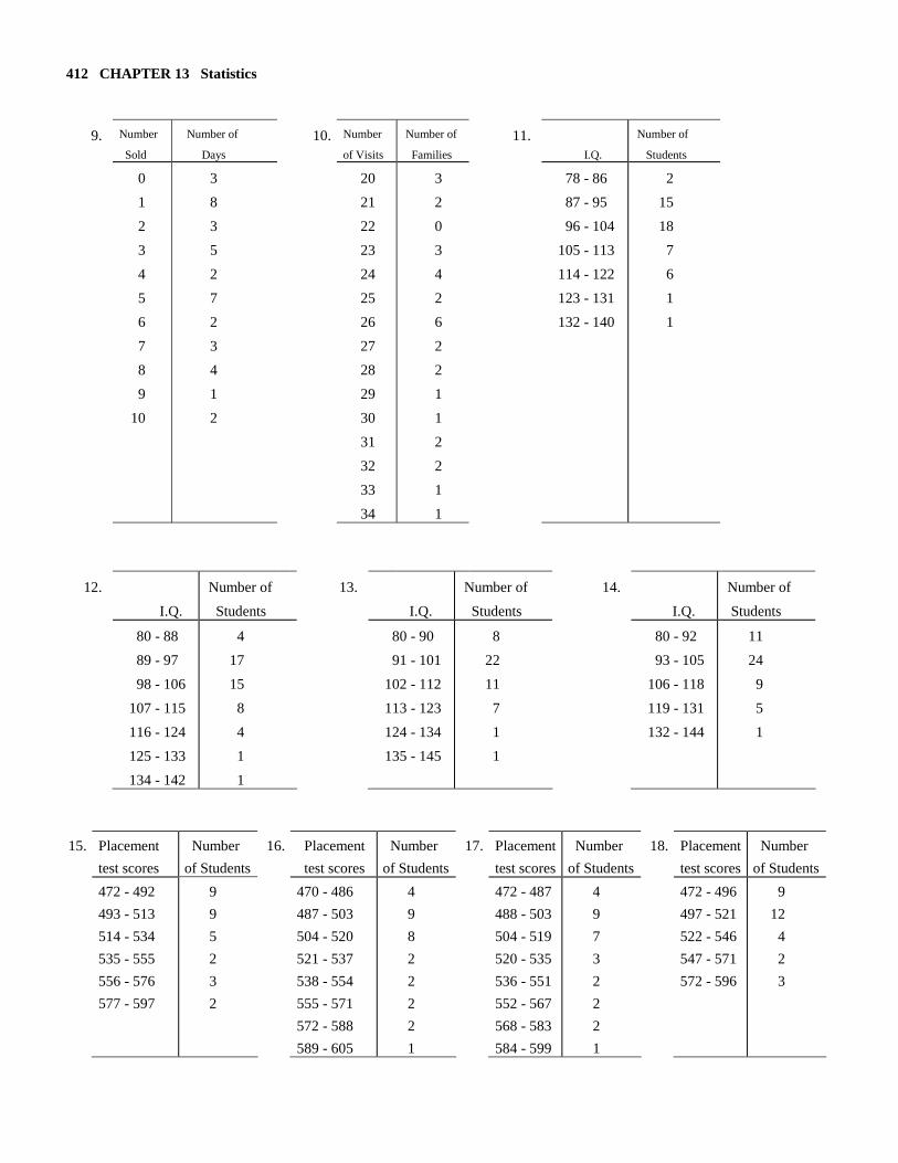
412 CHAPTER 13 Statistics
9. Number
Sold
Number of
Days 10. Number
of Visits
Number of
Families 11.
I.Q.
Number of
Students
0
1
2
3
4
5
6
7
8
9
10
3
8
3
5
2
7
2
3
4
1
2
20
21
22
23
24
25
26
27
28
29
30
31
32
33
34
3
2
0
3
4
2
6
2
2
1
1
2
2
1
1
78 - 86
87 - 95
96 - 104
105 - 113
114 - 122
123 - 131
132 - 140
2
15
18
7
6
1
1
12.
I.Q.
Number of
Students
13.
I.Q.
Number of
Students
14.
I.Q.
Number of
Students
80 - 88
89 - 97
98 - 106
107 - 115
116 - 124
125 - 133
134 - 142
4
17
15
8
4
1
1
80 - 90
91 - 101
102 - 112
113 - 123
124 - 134
135 - 145
8
22
11
7
1
1
80 - 92
93 - 105
106 - 118
119 - 131
132 - 144
11
24
9
5
1
15. Placement
test scores
Number
of Students
16. Placement
test scores
Number
of Students
17. Placement
test scores
Number
of Students
18. Placement
test scores
Number
of Students
472 - 492
493 - 513
514 - 534
535 - 555
556 - 576
577 - 597
9
9
5
2
3
2
470 - 486
487 - 503
504 - 520
521 - 537
538 - 554
555 - 571
572 - 588
589 - 605
4
9
8
2
2
2
2
1
472 - 487
488 - 503
504 - 519
520 - 535
536 - 551
552 - 567
568 - 583
584 - 599
4
9
7
3
2
2
2
1
472 - 496
497 - 521
522 - 546
547 - 571
572 - 596
9
12
4
2
3

SECTION 13.3 413
19. Circulation (thousands)
Number of Newspapers
20. Circulation (thousands)
Number of Newspapers
21. Circulation (thousands)
Number of Newspapers
209 - 458 459 - 708 709 - 958 959 - 1208
1209 - 1458 1459 - 1708 1709 - 1958 1959 - 2208
36 8 3 1 0 0 1 1
205 - 414 415 - 624 625 - 834 835 - 1044
1045 - 1254 1255 - 1464 1465 - 1674 1675 - 1884 1885 - 2094 2095 - 2304
35 8 3 1 1 0 0 1 0 1
209 - 408 409 - 608 609 - 808 809 - 1008 1009 - 1208 1209 - 1408 1409 - 1608 1609 - 1808 1809 - 2008 2009 - 2208
34 9 3 1 1 0 0 1 0 1
22. Circulation (thousands)
Number of Newspapers
23. Population (millions)
Number of Counties
24. Population (millions)
Number of Counties
209 - 358 359 - 508 509 - 658 659 - 808 809 - 958 959 - 1108
1109 - 1258 1259 - 1408 1409 - 1558 1559 - 1708 1709 - 1858 1859 - 2008 2009 - 2158
30 9 4 3 1 0 1 0 0 0 1 0 1
1.4 - 2.1 2.2 - 2.9 3.0 - 3.7 3.8 - 4.5 4.6 - 5.3 5.4 - 6.1 6.2 - 6.9 7.0 - 7.7 7.8 - 8.5 8.6 - 9.3 9.4 - 10.1
15 6 2 0 0 1 0 0 0 0 1
1.0 - 2.7 2.8 - 4.5 4.6 - 6.3 6.4 - 8.1 8.2 - 9.9
19 4 1 0 1
25. Population
(millions)
Number of
Counties
26. Population
(millions)
Number of
Counties
27. Price
($)
Number of
States
1.0 - 2.5
2.6 - 4.1
4.2 - 5.7
5.8 - 7.3
7.4 - 8.9
9.0 - 10.5
19
4
1
0
0
1
1.4 - 2.9
3.0 - 4.5
4.6 - 6.1
6.2 - 7.7
7.8 - 9.3
9.4 - 10.9
21
2
1
0
0
1
0.35 - 0.44
0.45 - 0.54
0.55 - 0.64
0.65 - 0.74
0.75 - 0.84
0.85 - 0.94
0.95 - 1.04
1.05 - 1.14
1.15 - 1.24
1.25 - 1.34
1.35 - 1.44
1.45 - 1.54
6
10
11
3
2
4
1
2
2
1
0
1

414 CHAPTER 13 Statistics
28. Price
($)
Number of
States
29. Price
($)
Number of
States
30. Price
($)
Number of
States
0.35 - 0.45
0.46 - 0.56
0.57 - 0.67
0.68 - 0.78
0.79 - 0.89
0.90 - 1.00
1.01 - 1.11
1.12 - 1.22
1.23 - 1.33
1.34 - 1.44
1.45 - 1.55
7
13
8
2
5
2
2
1
2
0
1
0.35 - 0.54
0.55 - 0.74
0.75 - 0.94
0.95 - 1.14
1.15 - 1.34
1.35 - 1.54
16
14
6
3
3
1
0.35 - 0.48
0.49 - 0.62
0.63 - 0.76
0.77 - 0.90
0.91 - 1.04
1.05 - 1.18
1.19 - 1.32
1.33 - 1.46
12
12
6
6
1
3
2
1
31. February, since it has the fewest number of days 32. a) Did You Know?, page 762: There are 6 F’s.
b) Answers will vary. Exercise Set 13.4
1. Answers will vary. 2. a) Observed values b) Frequency
3. Answers will vary. 4. Answers will vary. 5. a) Answers will vary. b)
6. a) Answers will vary. b)
Children in Selected Families
0
1
2
3
4
5
6
7
8
0 1 2 3 4 5 6 7
Number of Children
Nu
mb
er o
f F
amili
es
Number of Sick Days Taken Last Year
012345678
0 1 2 3 4 5 6 7
Sick Days Taken
Num
ber
of P
eopl
e

SECTION 13.4 415
Permits for New Houses, Number of Bedrooms
5 or more bedrooms
14.7%2 bedrooms
30.3%
3 bedrooms38.3%
4 bedrooms16.7%
7. a) Answers will vary.
b) Observed Values Frequency 45 3 46 0 47 1 48 0 49 1 50 1 51 2
8. Observed Values Frequency
16 1 17 2 18 1 19 1 20 0 21 1 22 2 23 1 24 1 25 2
9. Occasionally: ( )0.59 500 295=
Most Times: ( )0.25 500 125=
Every Time: ( )0.07 500 35=
Never: ( )0.09 500 45=
10. Retail: ( )0.518 700 362.6 363= ≈
Services: ( )0.259 700 181.3 181= ≈
Other: ( )0.223 700 156.1 156= ≈
11. Travelocity: 175
0.35 35%500
= = Priceline: 85
0.17 17%500
= =
Expedia: 125
0.25 25%500
= = Other: 115
0.23 23%500
= =
12. 2 bedrooms: 182
0.303 30.3%600
= ≈ 4 bedrooms: 100
0.16 16.7%600
= ≈
3 bedrooms: 230
0.383 38.3%600
= ≈ 5 or more bedrooms: 88
0.146 14.7%600
= ≈
Using Online Travel Websites
Expedia25%
Priceline17%
Other23%
Travelocity35%

416 CHAPTER 13 Statistics
13. a) and b)
14. a) and b)
15. a) and b)
16. a) and b)
Height of Male High School Seniors
0123456789
10
64 65 66 67 68 69 70 71 72
Height (inches)
Nu
mb
er o
f M
ales
Age of People Attending a Jazz Concert
0123456789
10
17 18 19 20 21 22 23 24
Age
Nu
mb
er o
f P
eop
le
DVDs Owned
0123456789
1011
9.5 17.5 25.5 33.5 41.5 49.5 57.5
Number of DVDs
Nu
mb
er o
f P
eop
le
Annual Salaries of Management at the X-Chek Corp.
0123456789
32.5 38.5 44.5 50.5 56.5 62.5 68.5
Salaries (in $1000)
Nu
mbe
r of
Peo
ple

SECTION 13.4 417
17. a) The total number of people surveyed: e) Number of Soft Drinks Purchased Number of People 2 + 7 + 8 + 5 + 4 + 3 + 1 = 30 0 2 b) Four people purchased four soft drinks. 1 7 c) The modal class is 2 because more people 2 8 purchased 2 soft drinks than any other number of soft drinks. 3 5 d) Two people bought 0 soft drinks 0 4 4 Seven people bought 1 soft drink 7 5 3 Eight people bought 2 soft drinks 16 6 1 Five people bought 3 soft drinks 15 Four people bought 4 soft drinks 16 Three people bought 5 soft drinks 15 One person bought 6 soft drinks 6 Total number of soft drinks purchased: 75 18) a) The total number of students surveyed: 2 + 4 + 6 + 8 + 7 + 3 + 1 = 31
b) Since there are 51 units between class midpoints, each class width must also be 51 units. 650 is the midpoint of the first class and there must be 25 units below it and 25 units above it. Therefore, the first class is 625 - 675. The second class will be 676 - 726.
c) Six d) The class mark of the modal class is $803 because more students had an annual car insurance premium of $778 - $828 than any other annual car insurance premium.
e) Price Number of Students 625 - 675 2 676 - 726 4 727 - 777 6 778 - 828 8 829 - 879 7 880 - 930 3 931 - 981 0 982 - 1032 1 19. a) 7 calls b) Adding the number of calls responded to in 6, 5, 4, or 3 minutes gives: 4 + 7 + 3 + 2 = 16 calls c) The total number of calls surveyed: 2 + 3 + 7 + 4 + 3 + 8 + 6 + 3 = 36 d) Response Time (min.) Number of Calls 3 2 4 3 5 7 6 4 7 3 8 8 9 6 10 3
e)
Response Time for Selected Emergency Calls in Phoenix
012345678
3 4 5 6 7 8 9 10
Response Time (minutes)
Num
ber
of C
alls

418 CHAPTER 13 Statistics
20. a) 8 families b) At least six times means six or more times. Adding the families that went 6, 7, 8, 9, or 10 times gives 11 + 9 + 3 + 0 + 1 = 24 families c) Total number of families surveyed: 4 + 2 + 8 + 8 + 6 + 11 + 9 + 3 + 0 + 1 = 52 families d) Number of Visits Number of Families 1 4 2 2 3 8 4 8 5 6 6 11 7 9 8 3 9 0 10 1
e)
21.
22.
23. 1 5 represents 15 1 0 5 7 2 4 4 3 6 0 3 4 8 5 2 5 8 5 3 4 6 0 2 0
24. 1 2 represents 12 0 3 8 2 5 1 2 8 2 5 9 3 7 6 2 5 1 7 2 3 3 3 4 4 1
Number of Visits Selected Families Have Made to the San Diego Zoo
0123456789
1011
1 2 3 4 5 6 7 8 9 10
Number of Visits
Num
ber
of F
amili
es
0
1
2
3
4
5
6
12 19 26 33 40 47
Class
Fre
quen
cy
0
1
2
3
4
5
6
7
44.5 54.5 64.5 74.5 84.5 94.5
Class
Fre
qu
ency

SECTION 13.4 419
25. a) Salaries (in $1000) Number of Companies 27 1 28 7 29 4 30 3 31 2 32 3 33 3 34 2
b) and c)
d) 2 3 represents 23 2 7 8 8 8 8 8 8 8 9 9 9 9 3 0 0 0 1 1 2 2 2 3 3 3 4 4 26. a) Age Number of People 20 - 24 9 25 - 29 6 30 - 34 10 35 - 39 6 40 - 44 5 45 - 49 4
b) and c)
d) 2 3 represents 23 2 0 1 1 2 3 3 3 4 4 5 5 6 7 8 8 3 0 0 0 1 1 2 3 4 4 4 5 5 5 7 8 9 4 0 0 0 2 4 5 5 6 7 27. a) Advertising Spending Number of (millions of dollars) Companies
b) and c)
597 - 905 19 906 - 1214 14 1215 - 1523 7 1524 - 1832 3 1833 - 2141 2 2142 - 2450 3 2451 - 2759 1 2760 - 3068 0 3069 - 3377 1
Starting Salaries for 25 Different Social Workers
0
1
2
3
4
5
6
7
8
27 28 29 30 31 32 33 34
Salaries, in $1000
No.
of S
oc. W
orke
rs
Age of 40 People Attending a Broadway Show
0123456789
10
22 27 32 37 42 47
Age
Num
ber
of P
eopl
e
Advertising Spending
02468
101214161820
751 1060 1369 1678 1987 2296 2605 2914 3223
Spending (millions of dollars)
Num
ber
of C
ompa
nies

420 CHAPTER 13 Statistics
28. a) Age Number of Ambassadors 40 - 44 9 45 - 49 6 50 - 54 10 55 - 59 6 60 - 64 5 65 - 69 4
b) and c)
29. a) - e) Answers will vary. 30. a) - e) Answers will vary.
Exercise Set 13. 5
1. Ranked data are data listed from the lowest value to the highest value or from the highest value to the lowest value. 2. The mean is the balancing point of a set of data. It is the sum of the data divided by the number of pieces of data. 3. The median is the value in the middle of a set of ranked data. To find the median, rank the data and select the value in the middle. 4. The midrange is the value half way between the lowest and highest values. To find the midrange, add the lowest and highest values and divide the sum by 2.
5. The mode is the most common piece of data. The piece of data that occurs most frequently is the mode. 6. The mode may be used when you are primarily interested in the most popular value, or the one that occurs most often,
for example, when buying clothing for a store. 7. The median should be used when there are some values that differ greatly from the rest of the values in the set, for
example, salaries. 8. The midrange should be used when the item being studied is constantly fluctuating, for example, daily temperature. 9. The mean is used when each piece of data is to be considered and "weighed" equally, for example, weights of adult males. 10. a) x b) µ
mean median mode midrange
11. 99
119
= 10 10 5 23
142
+ =
12. 550
5510
= 15 15
152
+ = 15 9 370
189.52
+ =
13. 485
69.37
≈ 72 none 42 90
662
+ =
14. 58
8.37
≈ 8 8 5 12
8.52
+ =
15. 88
64 = 82
97 =+ none 8
2
151 =+
16. 9.727
510 ≈ 60 none 852
14030 =+
Ages of U.S. Ambassadors
0123456789
10
42 47 52 57 62 67
Ages
Num
ber
of A
mba
ssad
ors

SECTION 13.5 421
mean median mode midrange
17. 1.139
118 ≈ 11 1 5.182
361 =+
18. 6.614
92 ≈ 42
44 =+ 1 and 4 11
2
211 =+
19. 9.118
95 ≈ 5.122
1312 =+ 13 5.11
2
176 =+
20. 106
60 = 102
155 =+ 5 and 15 10
2
155 =+
21. 65
6.510
= 5 5
52
+ = 3 and 5 2 19
10.52
+ =
22. $469
$677
= $59 none $25 $140
$82.502
+ =
23. a) 9.47
34 ≈ 5 5 62
111 =+
b) 3.57
37 ≈ 5 5 62
111 =+
c) Only the mean
d) 7.47
33 ≈ 5 5 5.52
101 =+
The mean and the midrange
24. Answers will vary. The National Center for Health uses the median for averages in this exercise.
25. A 79 mean average on 10 quizzes gives a total of 790 points. An 80 mean average on 10 quizzes requires a total of
800 points. Thus, Jim missed a B by 10 points not 1 point.
26. a) Mean: $361,000
$36,10010
= b) Median: $27,000 $28,000
$27,5002
+ =
c) Mode: $26,000 d) Midrange:
$24,000 $81,000$52,500
2
+ =
e) The median, since it is lower f) The mean, since it is higher
27. a) Mean: 87.7
8.8 million10
≈ b) Median: 7.8 8.2
8.0 million2
+ =
c) Mode: none d) Midrange:
4.6 19.712.2 million
2
+ ≈
28. a) Mean: $14,810
$1234.1712
≈ b) Median: $1230 $1250
$12402
+ =
c) Mode: $850 d) Midrange:
$850 $1900$1375
2
+ =

422 CHAPTER 13 Statistics
29. a) Mean: $55.9
$5.1 billion11
≈ b) Median: $2.3 billion
c) Mode: $2.3 billion and $1.5 billion d) Midrange:
$1.5 $26.5$14 billion
2
+ =
e) Answers will vary. 30. Let =x the sum of his scores
765
x =
( )76 5 380x = =
31. Let =x the sum of his scores
856
x =
( )85 6 510x = =
32. One example is 1, 1, 2, 5, 6. Mode = 1, Median = 2, Mean 35
15 ==
33. One example is 72, 73, 74, 76, 77, 78.
Mean: 450
756
= , Median: 74 76
752
+ = , Midrange: 72 78
752
+ =
34. One example is 80, 82, 84, 88, 94, 100.
Mean: 528
886
=
35. a) Yes b) Cannot be found since we do not know the middle two numbers in the ranked list c) Cannot be found without knowing all of the numbers d) Yes
e) Mean: 200120
000,24 = ; Midrange: 50 500
2752
+ =
36. A total of 400580 =× points are needed for a grade of B. Jorge earned 73 + 69 + 85 + 80 = 307 points on his first four exams. Thus, he needs 400 - 307 = 93 or higher to get a B.
37. a) For a mean average of 60 on 7 exams, she must have a total of 420760 =× points. Sheryl presently has 49 + 72 + 80 + 60 + 57 + 69 = 387 points. Thus, to pass the course, her last exam must be 420 - 387 = 33 or greater. b) A C average requires a total of 490770 =× points. Sheryl has 387. Therefore, she would need 490 - 387 = 103 on her last exam. If the maximum score she can receive is 100, she cannot obtain a C. c) For a mean average of 60 on 6 exams, she must have a total of 360660 =× points. If the lowest score on an exam
she has already taken is dropped, she will have a total of 72 + 80 + 60 + 57 + 69 = 338 points. Thus, to pass the course, her last exam must be 360 - 338 = 22 or greater.
d) For a mean average of 70 on 6 exams, she must have a total of 420670 =× points. If the lowest score on an exam she has already taken is dropped, she will have a total of 338 points. Thus, to obtain a C, her last exam must be
420 - 338 = 82 or greater. 38. The mode is the only measure which must be an actual piece of data since it is the most frequently occurring piece of
data.
39. One example is 1, 2, 3, 3, 4, 5 changed to 1, 2, 3, 4, 4, 5.
First set of data: Mean: 18
36
= , Median: 3 3
32
+ = , Mode: 3
Second set of data: Mean: 19
3.166
= , Median: 3 4
3.52
+ = , Mode: 4

SECTION 13.5 423
40. The mean changes from 5.16
9 = to 6.16
10 = . The mode changes from no mode to a mode of 1.
The midrange changes from 5.12
3 = to 22
4 = .
41. No, by changing only one piece of the six pieces of data you cannot alter both the median and the midrange. 42. Let =x sum of the values
20.8512
=x
( ) 40.1022$1220.85 ==x
40.1049$74$47$40.1022$ =+−
45.87$12
40.1049 = is the correct mean
43. The data must be arranged in either ascending or descending order. 44. She scored above approximately 73% of all the students who took the test. 45. He is taller than approximately 35% of all kindergarten children. 46. About 25% of the workers earn $20,750 or less.
47. a) 2 Median $430Q = =
b) $290, $300, $300, $330, $350, $350, $350, $350, $350, $400
1
$350 $350Median of the data listed below $350
2Q
+= = =
c) $450, $450, $500, $600, $650, $650, $700, $700, $750, $800
3
$650 $650Median of the data listed above $650
2Q
+= = =
48. a) 2
27 28Median 27.5
2Q
+= = = ¢
b) 17¢, 17¢, 20¢, 21¢, 24¢, 25¢, 27¢, 27¢, 27¢, 27¢
1
24 25Median of the data listed below 24.5
2Q
+= = = ¢
c) 28¢, 28¢, 28¢, 28¢, 31¢, 33¢, 38¢, 74¢, 80¢, 81¢
3
31 33Median of the data listed above 32
2Q
+= = = ¢
49. Second quartile, median 50. a) No, the percentile only indicated relative position of the score and not the value of it.
b) Yes, a higher percentile indicates a higher relative position in the respective population. Thus, Kendra was in a better relative position. 51. a) $490 b) $500 c) 25% d) 25% e) 17% f) 100 × $510 = $51,000
52. a) 87
56 = , 5.64
26 = , 25
10 = , 105
50 = , 666
396 =
b) 5.185
5.92 = c) 926.1927
538 ≈ d) No
424 CHAPTER 13 Statistics
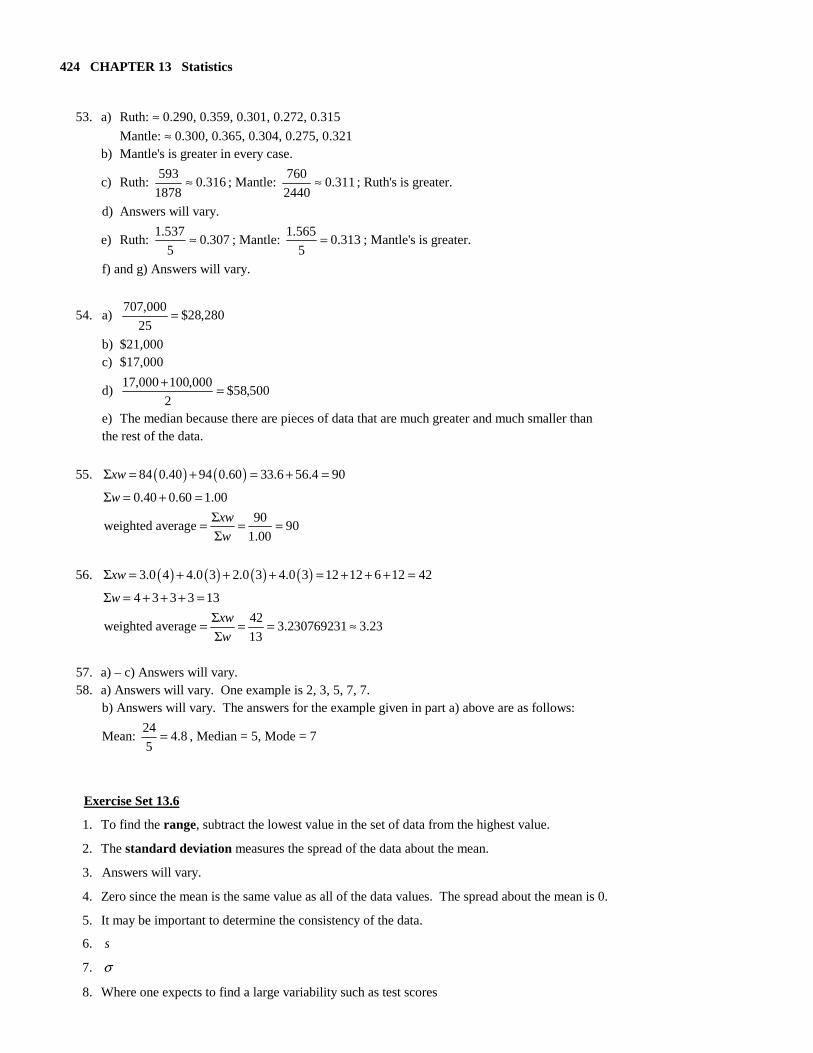
53. a) Ruth: ≈ 0.290, 0.359, 0.301, 0.272, 0.315
Mantle: ≈ 0.300, 0.365, 0.304, 0.275, 0.321 b) Mantle's is greater in every case.
c) Ruth: 316.01878
593 ≈ ; Mantle: 311.02440
760 ≈ ; Ruth's is greater.
d) Answers will vary.
e) Ruth: 307.05
537.1 ≈ ; Mantle: 313.05
565.1 = ; Mantle's is greater.
f) and g) Answers will vary.
54. a) 280,28$25
000,707 =
b) $21,000 c) $17,000
d) 500,58$2
000,100000,17 =+
e) The median because there are pieces of data that are much greater and much smaller than the rest of the data.
55. ( ) ( )84 0.40 94 0.60 33.6 56.4 90xwΣ = + = + =
0.40 0.60 1.00
90weighted average 90
1.00
w
xw
w
Σ = + =Σ= = =Σ
56. ( ) ( ) ( ) ( )3.0 4 4.0 3 2.0 3 4.0 3 12 12 6 12 42xwΣ = + + + = + + + =
4 3 3 3 13
42weighted average 3.230769231 3.23
13
w
xw
w
Σ = + + + =Σ= = = ≈Σ
57. a) – c) Answers will vary. 58. a) Answers will vary. One example is 2, 3, 5, 7, 7. b) Answers will vary. The answers for the example given in part a) above are as follows:
Mean: 24
4.85
= , Median = 5, Mode = 7
Exercise Set 13.6
1. To find the range, subtract the lowest value in the set of data from the highest value.
2. The standard deviation measures the spread of the data about the mean.
3. Answers will vary.
4. Zero since the mean is the same value as all of the data values. The spread about the mean is 0.
5. It may be important to determine the consistency of the data.
6. s
7. σ
8. Where one expects to find a large variability such as test scores

SECTION 13.6 425
9. In manufacturing or anywhere else where a minimum variability is desired
10. The first set of data will have the greater standard deviation because the scores have a greater
spread about the mean.
11. They would be the same since the spread of data about each mean is the same.
12. The sum of the values in the (Data − Mean)2 column will always be greater than or equal to 0.
13. a) The grades will be centered about the same number since the mean, 75.2, is the same for both classes.
b) The spread of the data about the mean is greater for the evening class since the standard deviation is greater for the evening class. 14. Answers will vary. 15. Range = 13 − 2 = 11 16. Range = 16 − 8 = 8
35
75
x = = 66
116
x = =
x xx − ( )2xx − x xx − ( )2xx −
7 0 0 10 -1 1 5 -2 4 10 -1 1 2 -5 25 14 3 9 8 1 1 16 5 25 13 6 36 8 -3 9 0 66 8 -3 9 0 54
06.45.16,5.164
66 ≈== s 29.38.10,8.105
54 ≈== s
17. Range = 126 − 120 = 6 18. Range = 12 − 0 = 12
861
1237
x = = 70
710
x = =
x xx − ( )2xx − x xx − ( )2xx −
120 -3 9 3 -4 16 121 -2 4 7 0 0 122 -1 1 8 1 1 123 0 0 12 5 25 124 1 1 0 -7 49 125 2 4 9 2 4 126 3 9 11 4 16 0 28 12 5 25 6 -1 1 2 -5 25 0 162
16.267.4,67.46
28 ≈=≈ s 162
18, 18 4.249
s= = ≈

426 CHAPTER 13 Statistics
19. Range = 15 − 4 = 11 20. Range = 9 − 9 = 0
60
106
x = = Since all pieces of data are identical,
x xx − ( )2xx − the standard deviation is 0.
4 -6 36 8 -2 4 9 -1 1 11 1 1 13 3 9 15 5 25 0 76
76
15.2, 15.2 3.905
s= = ≈
21. Range = 12 − 7 = 5 22. Range = 64 − 40 = 24
97
63 ==x 538
424 ==x
x xx − ( )2xx − x xx − ( )2xx −
7 -2 4 52 -1 1 9 0 0 50 -3 9 7 -2 4 54 1 1 9 0 0 59 6 36 9 0 0 40 -13 169
10 1 1 43 -10 100 12 3 9 64 11 121 0 18 62 9 81 0 518
73.13,36
18 ≈== s 60.874,747
518 ≈== s
23. Range = 50 − 18 = $32 24. Range = 28 − 1 = 27
36$10
360 ==x 84
127
x = =
x xx − ( )2xx − x xx − ( )2xx −
28 -8 64 10 -2 4 28 -8 64 23 11 121 50 14 196 28 16 256 45 9 81 4 -8 64 30 -6 36 1 -11 121 45 9 81 6 -6 36 48 12 144 12 0 0 18 -18 324 0 602 45 9 81 23 -13 169 0 1240
74.11$78.137,78.1379
1240 ≈=≈ s 602
100.33, 100.33 10.026
s≈ = ≈

SECTION 13.6 427
25. Range = 200 − 50 = $150 26. Range = 300 − 35 = $265
1100
$11010
x = = 980
$1407
x = =
x xx − ( )2xx − x xx − ( )2xx −
50 -60 3600 60 -80 6400 120 10 100 100 -40 1600 130 20 400 85 -55 3025 60 -50 2500 35 -105 11,025 55 -55 3025 250 110 12,100 75 -35 1225 150 10 100 200 90 8100 300 160 25,600 110 0 0 0 59,850 125 15 225 175 65 4225 0 23,400
23, 400
2600, 2600 $50.999
s= = ≈ 59,850
9975, 9975 $99.876
s= = ≈
27. a) Range = 68 - 5 = $63
204
$346
x = =
x xx − ( )2xx −
32 -2 4 60 26 676 14 -20 400 25 -9 81 5 -29 841 68 34 1156 0 3158
13.25$6.631,6.6315
3158 ≈== s
b) New data: 42, 70, 24, 35, 15, 78 The range and standard deviation will be the same. If each piece of data is increased by the same number, the range and standard deviation will remain the same. c) Range = 78 - 15 = $63
264
$446
x = =
x xx − ( )2xx −
42 -2 4 70 26 676 24 -20 400 35 -9 81 15 -29 841 78 34 1156 0 3158
13.25$6.631,6.6315
3158 ≈== s
The answers remain the same.

428 CHAPTER 13 Statistics
28. a) - c) Answers will vary.
d) If each piece of data is increased, or decreased, by n, the mean is increased, or decreased, by n. The standard deviation remains the same.
e) The mean of the first set of numbers is 97
63 = . The mean of the second set is 5997
4193 = .
Standard deviation of first set Standard deviation of second set
x xx − ( )2xx − x xx − ( )2xx −
6 -3 9 596 -3 9 7 -2 4 597 -2 4 8 -1 1 598 -1 1 9 0 0 599 0 0 10 1 1 600 1 1 11 2 4 601 2 4 12 3 9 602 3 9 0 28 0 28
16.267.4,67.46
28 ≈== s 16.267.4,67.46
28 ≈== s
29. a) - c) Answers will vary. d) If each number in a distribution is multiplied by n, both the mean and standard deviation of the new distribution
will be n times that of the original distribution. e) The mean of the second set is 4 5 20× = , and the standard deviation of the second set is 2 5 10× = . 30. a) Same b) More 31. a) The standard deviation increases. There is a greater spread from the mean as they get older.
b) 133 lb≈
c) 175 90
21.25 21 lb4
− = ≈
d) The mean weight is about 100 pounds and the normal range is about 60 to 140 pounds. e) The mean height is about 62 inches and the normal range is about 53 to 68 inches. f) 100% - 95% = 5% 32. a) and b) Answers will vary.
c) Baseball: 172
$17.20 million10
=
NFL: 1216
$12.16 million10
=

SECTION 13.6 429
32. d) Baseball Mean $17.2 million≈
NFL Mean $12.2 million≈ Baseball NFL
x xx − ( )2xx − x xx − ( )2xx −
22 4.8 23.04 15.4 3.2 10.24 20 2.8 7.84 13.3 1.1 1.21 18.7 1.5 2.25 13.0 0.8 0.64 17.2 0 0 12.0 -0.2 0.04 16 -1.2 1.44 11.7 -0.5 0.25 15.7 -1.5 2.25 11.7 -0.5 0.25 15.7 -1.5 2.25 11.4 -0.8 0.64 15.6 -1.6 2.56 11.3 -0.9 0.81 15.6 -1.6 2.56 11.3 -0.9 0.81 15.5 -1.7 2.89 10.5 -1.7 2.89
47.08 17.78
47.08
5.23, 5.23 $2.29 million9
s≈ = ≈ 17.78
1.98, 1.98 $1.41 million9
s≈ = ≈
33. a) East West Number of oil changes Number of Number of oil changes Number of made days made days 15-20 2 15-20 0 21-26 2 21-26 0 27-32 5 27-32 6 33-38 4 33-38 9 39-44 7 39-44 4 45-50 1 45-50 6 51-56 1 51-56 0 57-62 2 57-62 0 63-68 1 63-68 0 b) c) They appear to have about the same mean since they are both centered around 38. d) The distribution for East is more spread out. Therefore, East has a greater standard deviation.
e) East: 3825
950 = , West: 3825
950 =
Number of Oil Changes Made Daily at East Store
01234567
17.5 23.5 29.5 35.5 41.5 47.5 53.5 59.5 65.5
Number Made
Num
ber
of D
ays
Number of Oil Changes Made Daily at West Store
0123456789
17.5 23.5 29.5 35.5 41.5 47.5 53.5 59.5 65.5
Number Made
Num
ber
of D
ays

430 CHAPTER 13 Statistics
33. f) East West
x xx − ( )2xx − x xx − ( )2xx −
33 -5 25 38 0 0 30 -8 64 38 0 0 25 -13 169 37 -1 1 27 -11 121 36 -2 4 40 2 4 30 -8 64 44 6 36 45 7 49 49 11 121 28 -10 100 52 14 196 47 9 81 42 4 16 30 -8 64 59 21 441 46 8 64 19 -19 361 38 0 0 22 -16 256 39 1 1 57 19 361 40 2 4 67 29 841 34 -4 16 15 -23 529 31 -7 49 41 3 9 45 7 49
43 5 25 29 -9 81 27 -11 121 38 0 0 42 4 16 38 0 0 43 5 25 39 1 1 37 -1 1 37 -1 1 38 0 0 42 4 16 31 -7 49 46 8 64 32 -6 36 31 -7 49 35 -3 9 48 10 100 0 3832 0 858
3832
159.67, 159.67 12.6424
s≈ = ≈ 858
35.75, 35.75 5.9824
s= = ≈
34. Answers will vary.
35. 6, 6, 6, 6, 6 Exercise Set 13.7 1. A rectangular distribution is one where all the values have the same frequency. 2. A J-shaped distribution is one where the frequency is either constantly increasing or constantly decreasing.
3. A bimodal distribution is one where two nonadjacent values occur more frequently than any other values in a set of data.
4. A distribution skewed to the right is one that has "a tail" on its right. 5. A distribution skewed to the left is one that has "a tail" on its left. 6. A normal distribution is a bell-shaped distribution. 7. a) B b) C c) A 8. a) Yes, 36 b) B, since curve B is more spread out it has the higher standard deviation. 9. The distribution of outcomes from the roll of a die 10. Skewed left - a listing of test scores where most of the students did well and a few did poorly; Skewed right - number of cans of soda consumed in a day where most people consumed a few cans and a few people consumed many cans 11. J shaped right - consumer price index; J shaped left - value of the dollar 12. The distribution of heights of an equal number of males and females

SECTION 13.7 431
13. Normal 14. Rectangular 15. Skewed right 16. Bimodal
17. The mode is the lowest value, the median is greater than the mode, and the mean is greater than the median. The greatest frequency appears on the left side of the curve. Since the mode is the value with the greatest frequency, the mode would appear on the left side of the curve (where the
lowest values are). Every value in the set of data is considered in determining the mean. The values on the far right of the curve would increase the value of the mean. Thus, the value of the mean would be farther to the right than the mode. The median would be between the mode and the mean. 18. The mode is the highest value. The median is lower than the mode. The mean is the lowest value. 19. Answers will vary. 20. Answers will vary. 21. In a normal distribution the mean, median, and the mode all have the same value. 22. A z-score measures how far, in terms of standard deviation, a given score is from the mean. 23. A z-score will be negative when the piece of data is less than the mean.
24. Subtract the mean from the value of the piece of data and divide the difference by the standard deviation.
25. 0 26. a) ≈ 68% b) ≈ 95%
27. 0.500 28. 0.500 29. 0.477 + 0.341 = 0.818 30. 0.455 – 0.364 = 0.091 31. 0.500 – 0.466 = 0.034 32. 0.500 + 0.383 = 0.883
33. 0.500 − 0.463 = 0.037 34. 0.500 + 0.463 = 0.963
35. 0.500 − 0.481 = 0.019 36. 0.500 + 0.475 = 0.975
37. 0.500 − 0.447 = 0.053 38. 0.500 – 0.316 = 0.184
39. 0.261 = 26.1% 40. 0.294 – 0.060 = 0.234 = 23.4% 41. 0.410 + 0.488 = 0.898 = 89.8% 42. 0.500 − 0.471 = 0.029 = 2.9% 43. 0.500 + 0.471 = 0.971 = 97.1% 44. 0.500 − 0.496 = 0.004 = 0.4% 45. 0.500 + 0.475 = 0.975 = 97.5% 46. 0.484 − 0.264 = 0.22 = 22.0%
47. 0.466 − 0.437 = 0.029 = 2.9% 48. 0.484 + 0.500 = 0.984 = 98.4%
49. a) Jake, Sarah, and Carol scored above the mean because their z-scores are positive. b) Marie and Kevin scored at the mean because their z-scores are zero. c) Omar, Justin, and Kim scored below the mean because their z-scores are negative. 50. a) Sarah had the highest score because she had the highest z-score. b) Omar had the lowest score because he had the lowest z-score. 51. 0.500 = 50%
52. 14
14 18 41.00
4 4z
− −= = = −
26
26 18 82.00
4 40.341 0.477 0.818 81.8%
z−= = =
+ = =
53. 23
23 18 51.25
4 4z
−= = =
0.500 – 0.394 = 0.106 = 10.6%
432 CHAPTER 13 Statistics
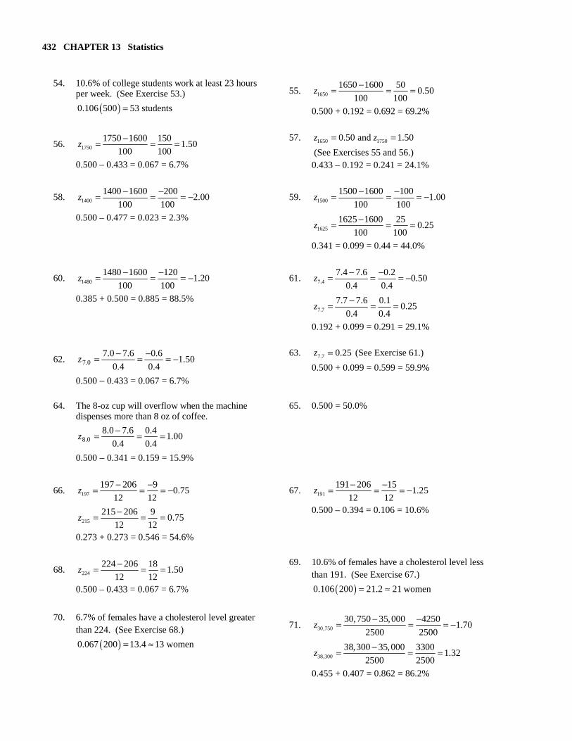
54. 10.6% of college students work at least 23 hours per week. (See Exercise 53.)
( )0.106 500 53 students=
55. 1650
1650 1600 500.50
100 100z
−= = =
0.500 + 0.192 = 0.692 = 69.2%
56. 1750
1750 1600 1501.50
100 100z
−= = =
0.500 – 0.433 = 0.067 = 6.7%
57. 1650 17500.50 and 1.50z z= =
(See Exercises 55 and 56.) 0.433 – 0.192 = 0.241 = 24.1%
58. 1400
1400 1600 2002.00
100 100z
− −= = = −
0.500 – 0.477 = 0.023 = 2.3%
59. 1500
1500 1600 1001.00
100 100z
− −= = = −
1625
1625 1600 250.25
100 100z
−= = =
0.341 = 0.099 = 0.44 = 44.0%
60. 1480
1480 1600 1201.20
100 100z
− −= = = −
0.385 + 0.500 = 0.885 = 88.5%
61. 7.4
7.4 7.6 0.20.50
0.4 0.4z
− −= = = −
7.7
7.7 7.6 0.10.25
0.4 0.4z
−= = =
0.192 + 0.099 = 0.291 = 29.1%
62. 50.14.0
6.0
4.0
6.70.70.7 −=−=−=z
0.500 − 0.433 = 0.067 = 6.7%
63. 7.7 0.25z = (See Exercise 61.)
0.500 + 0.099 = 0.599 = 59.9%
64. The 8-oz cup will overflow when the machine dispenses more than 8 oz of coffee.
00.14.0
4.0
4.0
6.70.80.8 ==−=z
0.500 − 0.341 = 0.159 = 15.9%
65. 0.500 = 50.0%
66. 197
197 206 90.75
12 12z
− −= = = −
215
215 206 90.75
12 12z
−= = =
0.273 + 0.273 = 0.546 = 54.6%
67. 191
191 206 151.25
12 12z
− −= = = −
0.500 – 0.394 = 0.106 = 10.6%
68. 224
224 206 181.50
12 12z
−= = =
0.500 – 0.433 = 0.067 = 6.7%
69. 10.6% of females have a cholesterol level less than 191. (See Exercise 67.)
( )0.106 200 21.2 21 women= ≈
70. 6.7% of females have a cholesterol level greater
than 224. (See Exercise 68.)
( )0.067 200 13.4 13 women= ≈
71. 30,750
30,750 35,000 42501.70
2500 2500z
− −= = = −
38,300
38,300 35,000 33001.32
2500 2500z
−= = =
0.455 + 0.407 = 0.862 = 86.2%

SECTION 13.7 433
72. At least 39,000 miles means 39,000 miles or more.
60.12500
4000
2500
000,35000,39000,39 ==−=z
0.500 − 0.445= 0.055 = 5.5%
73. The tires that last less than 30,750 miles will fail to live up to the guarantee.
30,750 1.70z = − (See Exercise 71.)
0.500 − 0.455 = 0.045 = 4.5%
74. 5.5% of tires will last at least 39,000 miles.
(See Exercise 72.)
( )0.055 200,000 11,000 tires=
75. 3.1
3.1 3.7 0.60.50
1.2 1.2z
− −= = = −
0.192 + 0.500 = 0.692 = 69.2%
76. 2.5
2.5 3.7 1.21.00
1.2 1.2z
− −= = = −
4.3
4.3 3.7 0.60.50
1.2 1.2z
−= = =
0.341 + 0.192 = 0.533 = 53.3%
77. 6.7
6.7 3.7 3.02.50
1.2 1.2z
−= = =
0.500 – 0.494 = 0.006 = 0.6%
78. 6.7 2.50z = (See Exercise 77.)
0.500 + 0.494 = 0.994 = 99.4%
79. 69.2% of the children are older than 3.1 years. (See Exercise 75.)
( )0.692 120 83.04 83 children= ≈
80. 53.3% of the children are between 2.5 and 4.3 years. (See Exercise 76.)
( )0.533 120 63.96 64 children= ≈
81. Customers will be able to claim a refund if they lose less than 5 lb.
10.281.0
7.1
81.0
7.655 −=−=−=z
0.500 − 0.482 = 0.018 = 1.8%
82. A motor will require repair or replacement if it breaks down in less than 8 years.
22.18.1
2.2
8.1
2.1088 −≈−=−=z
0.500 − 0.389 = 0.111 = 11.1%
83. The standard deviation is too large. There is too much variation.
84. A z-score of 1.8 or higher is required for an A. The area from the mean to 1.8 is 0.464.
Thus, 0.500 − 0.464 = 0.036 = 3.6% will receive an A. A z-score between 1.8 and 1.1 is required for a B. The areas from the mean to these z-scores are
0.464 and 0.364, respectively. Thus, 0.464 − 0.364 = 0.100 = 10.0% will receive a B. A z-score between 1.1 and -1.2 is required for a C. The areas from the mean to these z-scores are 0.364 and 0.385, respectively. Thus, 0.364 + 0.385 = 0.749 = 74.9% will receive a C. A z-score between -1.2 and -1.9 is required for a D. The areas from the mean to these z-scores are
0.385 and 0.471, respectively. Thus, 0.471 − 0.385 = 0.086 = 8.6% will receive a D. A z-score of -1.9 or lower is required for an F. The area from the mean to -1.9 is 0.471.
Thus, 0.500 − 0.471 = 0.029 = 2.9% will receive an F.

434 CHAPTER 13 Statistics
85. a) Katie: 4.22170
5208
2170
200,23408,28408,28 ==−=z
Stella: 7.12300
3910
2300
600,25510,29510,29 ==−=z
b) Katie. Her z-score is higher than Stella's z-score. This means her sales are further above the mean than Stella's sales.
86. a) 33.53.530
160 ≈==x
b) x xx − ( )2xx − x xx − ( )2xx − x xx − ( )2xx −
1 -4.33 18.75 4 -1.33 1.77 7 1.67 2.79 1 -4.33 18.75 4 -1.33 1.77 8 2.67 7.13 1 -4.33 18.75 4 -1.33 1.77 8 2.67 7.13 1 -4.33 18.75 5 -0.33 0.11 8 2.67 7.13 2 -3.33 11.09 6 0.67 0.45 8 2.67 7.13 2 -3.33 11.09 6 0.67 0.45 9 3.67 13.47 2 -3.33 11.09 6 0.67 0.45 9 3.67 13.47 2 -3.33 11.09 7 1.67 2.79 9 3.67 13.47 3 -2.33 5.43 7 1.67 2.79 10 4.67 21.81 3 -2.33 5.43 7 1.67 2.79 10 4.67 21.81 260.70
260.70 ÷ 29 ≈ 8.99 s = 8.99 ≈ 3.00 c) x + 1.1s = 5.33 + 1.1(3) = 8.63 x - 1.1s = 5.33 - 1.1(3) = 2.03 x + 1.5s = 5.33 + 1.5(3) = 9.83 x - 1.15s = 5.33 - 1.5(3) = 0.83 x + 2.0s = 5.33 + 2.0(3) = 11.33 x - 2.0s = 5.33 - 2.0(3) = -0.67 x + 2.5s = 5.33 + 2.5(3) = 12.83 x - 2.5s = 5.33 - 2.5(3) = -2.17
d) Between -1.1s and 1.1s or between scores of 2.03 and 8.63, there are 17 scores.
%7.5665.030
17 ≈=
Between -1.5s and 1.5s, or between scores of 0.83 and 9.83, there are 28 scores.
%3.9339.030
28 ≈=
Between -2.0s and 2.0s, or between scores of -0.67 and 11.33, there are 30 scores.
%100130
30 ==
Between -2.5s and 2.5s, or between scores of -2.17 and 12.83, there are 30 scores.
%100130
30 ==
e) Minimum % K = 1.1 K = 1.5 K = 2.0 K = 2.5
(For any distribution) 17.4% 55.6% 75% 84%
Normal distribution 72.8% 86.6% 95.4% 99.8%
Given distribution 56.7% 93.3% 100% 100%
f) The percent between -1.1s and 1.1s is too low to be considered a normal distribution.

SECTION 13.8 435
87. Answers will vary. 88. Using Table 13.7, the answer is 1.96. 89. Using Table 13.7, the answer is -1.18. 90. Answers will vary.
91. 0.77
0.3852
=
Using the table in Section 13.7, an area of 0.385 has a z-score of 1.20.
14.4 121.20
2.41.20
1.20 2.4
1.20 1.202
x xz
s
s
ss
s
−=
−=
=
=
=
Exercise Set 13.8
1. The correlation coefficient measures the strength of the relationship between the quantities.
2. The purpose of linear regression is to determine the linear relationship between two variables.
3. 1 4. -1 5. 0
6. A negative correlation indicates that as one quantity increases, the other quantity decreases.
7. A positive correlation indicates that as one quantity increases, the other quantity increases.
8. The line of best fit represents the line such that the sum of the vertical distances between the
points and the line is a minimum.
9. The level of significance is used to identify the cutoff between results attributed to chance and
results attributed to an actual relationship between the two variables.
10. A scatter diagram is a plot of data points.
11. No correlation 12. Weak negative
13. Strong positive 14. Strong negative
15. Yes, 0.76 0.684> 16. No, 0.43 0.537<
17. Yes, 0.73 0.707− > 18. No, 602.049.0 <−
19. No, 254.023.0 <− 20. No, 590.049.0 <−
21. No, 917.082.0 < 22. Yes, 959.096.0 >

436 CHAPTER 13 Statistics
Note: The answers in the remainder of this section may differ slightly from your answers, depending upon how your answers are rounded and which calculator you used. 23. a)
b) x y 2x 2y xy 4 6 16 36 24 5 9 25 81 45 6 11 36 121 66 7 11 49 121 77 10 13 100 169 130 32 50 226 528 342
( ) ( )
( ) ( )5 342 32 50 110
0.903106 1405 226 1024 5 528 2500
r−
= = ≈− −
c) Yes, 878.0903.0 > d) No, 959.0903.0 <
24. a)
b) x y 2x 2y xy 6 12 36 144 72 8 11 64 121 88 11 9 121 81 99 14 10 196 100 140 17 8 289 64 136 56 50 706 510 535
( ) ( )
( ) ( )5 535 56 50 125
0.891394 505 706 3136 5 510 2500
r− −= = ≈ −
− −
c) Yes, 878.0891.0 >− d) No, 959.0891.0 <−
0
2
4
6
8
10
12
14
0 2 4 6 8 10 12
x
y
x
y
0
2
4
6
8
10
12
14
0 2 4 6 8 10 12 14 16 18 20

SECTION 13.8 437
25. a)
b) x y 2x 2y xy 23 29 529 841 667 35 37 1225 1369 1295 31 26 961 676 806 43 20 1849 400 860 49 39 2401 1521 1911 181 151 6965 4807 5539
( ) ( )
( ) ( )228.0
12342064
364
801,2248075761,3269655
15118155395 ≈=−−
−=r
c) No, 878.0228.0 < d) No, 959.0228.0 <
26. a)
b) x y 2x 2y xy 90 3 8100 9 270 80 4 6400 16 320 60 6 3600 36 360 60 5 3600 25 300 40 5 1600 25 200 20 7 400 49 140 350 30 23,700 160 1590
( ) ( )
( ) ( )883.0
60700,19
960
9001606500,122700,236
3035015906 −≈−=−−
−=r
c) Yes, 811.0883.0 >− d) No, 917.0883.0 <−
0
5
10
15
20
25
30
35
40
45
0 5 10 15 20 25 30 35 40 45 50x
y
0
1
2
3
4
5
6
7
8
0 10 20 30 40 50 60 70 80 90
x
y
438 CHAPTER 13 Statistics
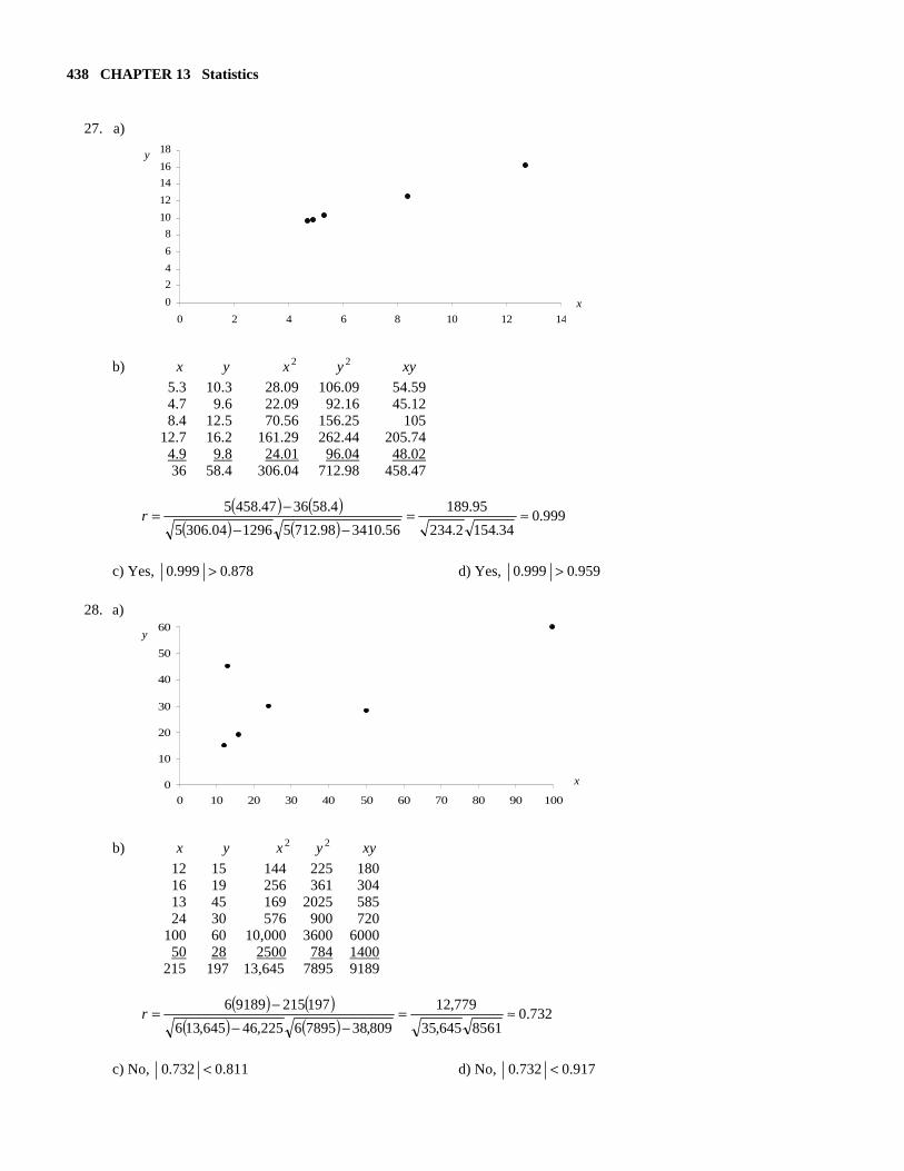
27. a)
b) x y 2x 2y xy 5.3 10.3 28.09 106.09 54.59 4.7 9.6 22.09 92.16 45.12 8.4 12.5 70.56 156.25 105 12.7 16.2 161.29 262.44 205.74 4.9 9.8 24.01 96.04 48.02 36 58.4 306.04 712.98 458.47
( ) ( )
( ) ( )999.0
34.1542.234
95.189
56.341098.7125129604.3065
4.583647.4585 ≈=−−
−=r
c) Yes, 878.0999.0 > d) Yes, 959.0999.0 >
28. a)
b) x y 2x 2y xy 12 15 144 225 180 16 19 256 361 304 13 45 169 2025 585 24 30 576 900 720 100 60 10,000 3600 6000 50 28 2500 784 1400 215 197 13,645 7895 9189
( ) ( )
( ) ( )732.0
8561645,35
779,12
809,3878956225,46645,136
19721591896 ≈=−−
−=r
c) No, 811.0732.0 < d) No, 917.0732.0 <
0
2
4
6
8
10
12
14
16
18
0 2 4 6 8 10 12 14
x
y
0
10
20
30
40
50
60
0 10 20 30 40 50 60 70 80 90 100
x
y

SECTION 13.8 439
x
y
29. a)
b) x y 2x 2y xy 100 2 10,000 4 200 80 3 6400 9 240 60 5 3600 25 300 60 6 3600 36 360 40 6 1600 36 240 20 8 400 64 160 360 30 25,600 174 1500
( ) ( )
( ) ( )968.0
144000,24
1800
9001746600,129600,256
3036015006 −≈−=−−
−=r
c) Yes, 811.0968.0 >− d) Yes, 917.0968.0 >−
30. a)
b) x y 2x 2y xy 90 90 8100 8100 8100 70 70 4900 4900 4900 65 65 4225 4225 4225 60 60 3600 3600 3600 50 50 2500 2500 2500 40 40 1600 1600 1600 15 15 225 225 225 390 390 25,150 25,150 25,150
( ) ( )
( ) ( )00.1
950,23950,23
950,23
100,152150,257100,152150,257
390390150,257 ==−−
−=r
c) Yes, 754.000.1 > d) Yes, 875.000.1 >
0
1
2
3
4
5
6
7
8
0 20 40 60 80 100
x
y
0
10
2030
40
50
60
7080
90
100
0 10 20 30 40 50 60 70 80 90 100

440 CHAPTER 13 Statistics
31. From # 23: ( ) ( )( )
5 342 32 50 1101.0
5 226 1024 106m
−= = ≈
−
( )110
50 32106 3.4, 1.0 3.4
5b y x
−= ≈ = +
32. From # 24: ( ) ( )( )
5 535 56 50 1250.3
5 706 3136 394m
− −= = ≈ −−
( )125
50 56394 13.6, 0.3 13.6
5b y x
−−= ≈ = − +
33. From # 25: ( ) ( )( ) 2.0
2064
364
761,3269655
15118155395 ≈=−
−=m
( )
8.232.0,8.235
1812064
364151
+=≈−
= xyb
34. From # 26: ( ) ( )
( ) 05.0700,19
960
500,122700,236
3035015906 −≈−=−
−=m
( )8.705.0,8.7
6
350700,19
96030
+−=≈
−−= xyb
35. From # 27: ( ) ( )
( ) 8.02.234
95.189
129604.3065
4.583647.4585 ≈=−
−=m
( )
8.58.0,8.55
362.234
95.1894.58
+=≈−
= xyb
36. From # 28: ( ) ( )( ) 4.0
645,35
779,12
225,46645,136
19721591896 ≈=−
−=m
( )
0.204.0,0.206
215645,35779,12
197+=≈
−= xyb
37. From # 29: ( ) ( )
( ) 1.0000,24
1800
600,129600,256
3036015006 −≈−=−
−=m
( )5.91.0,5.9
6
360000,24
180030
+−=≈
−−= xyb
38. From # 30: ( ) ( )( )
7 25,150 390 390 23,9501.0
7 25,150 152,100 23,950m
−= = =
−
( )390 1 390
0, 1.07
b y x−
= = =

SECTION 13.8 441
39. a) x y 2x 2y xy
8 15 64 225 120 20 28 400 784 560 9 20 81 400 180 15 25 225 625 375 16 28 256 784 448 2 5 4 25 10 70 121 1030 2843 1693
( ) ( )
( ) ( )6 1693 70 121 1688
0.9601280 24176 1030 4900 6 2843 14,641
r−
= = ≈− −
b) Yes, 0.960 0.811>
c) ( ) ( )
( )6 1693 70 121 1688
1.36 1030 4900 1280
m−
= = ≈−
, ( )1688
121 701280 4.8, 1.3 4.8
6b y x
−= ≈ = +
40. a) x y 2x 2y xy
321 13 103,041 169 4173 380 23 144,400 529 8740 350 16 122,500 256 5600 358 14 128,164 196 5012 378 19 142,884 361 7182 391 19 152,881 361 7429 2178 104 793,870 1872 38,136
( ) ( )
( ) ( )6 38,136 2178 104 2304
0.80819,536 4166 793,870 4,743,684 6 1872 10,816
r−
= = ≈− −
b) No, 0.808 0.811<
c) ( ) ( )( )
6 38,136 2178 104 23040.1
6 793,870 4,743,684 19,536m
−= = ≈
−,
( )2304104 2178
19,53625.5, 0.1 25.5
6b y x
−= ≈ − = −

442 CHAPTER 13 Statistics
41. a) x y 2x 2y xy
20 40 400 1600 800 40 45 1600 2025 1800 50 70 2500 4900 3500 60 76 3600 5776 4560 80 92 6400 8464 7360 100 95 10,000 9025 9500 350 418 24,500 31,790 27,520
( ) ( )
( ) ( )950.0
016,16500,24
820,18
724,174790,316500,122500,246
418350520,276 ≈=−−
−=r
b) Yes, 917.0950.0 >
c) ( ) ( )( ) 8.0
500,24
820,18
500,122500,246
418350520,276 ≈=−−=m ,
( )9.248.0,9.24
6
350500,24
820,18418
+=≈−
= xyb
42. a) x y 2x 2y xy
765 119 585,225 14,161 91,035 926 127 857,476 16,129 117,602 1145 150 1,311,025 22,500 171,750 842 119 708,964 14,161 100,198 1485 153 2,205,225 23,409 227,205 1702 156 2,896,804 24,336 265,512 6865 824 8,564,719 114,696 973,302
( ) ( )
( ) ( )6 973,302 6865 824 183,052
0.9254,260,089 92006 8,564,719 47,128,225 6 114,696 678,976
r−
= = ≈− −
b) Yes, 0.925 0.811>
c) ( ) ( )
( )6 973,302 6865 824 183,052
0.046 8,564,719 47,128,225 4,260,089
m−
= = ≈−
, ( )183,052
824 68654,260,089
88.2, 0.04 88.26
b y x−
= ≈ = +
d) ( )0.04 1500 88.2 148.2 148 mountain lionsy = + = ≈

SECTION 13.8 443
43. a) x y 2x 2y xy
20 8 400 64 160 12 10 144 100 120 18 12 324 144 216 15 9 225 81 135 22 6 484 36 132 10 15 100 225 150 20 7 400 49 140 12 18 144 324 216 129 85 2221 1023 1269
( ) ( )
( ) ( )782.0
9591127
813
722510238641,1622218
8512912698 −≈−=−−
−=r
b) Yes, 707.0782.0 >−
c) ( ) ( )( ) 7.0
1127
813
641,1622218
8512912698 −≈−=−−=m ,
( )3.227.0,3.22
8
1291127
81385
+−=≈
−−= xyb
d) ( ) 5.123.22147.0 =+−=y muggings
44. a) x y 2x 2y xy
00 15.0 0 225 0 01 15.3 1 234.09 15.3 02 15.5 4 240.25 31 03 15.8 9 249.64 47.4 04 16.1 16 259.21 64.4 05 16.3 25 265.69 81.5 15 94 55 1473.88 239.6
( ) ( )
( ) ( )6 239.6 15 94 27.6
0.998105 7.286 55 225 6 1473.88 8836
r−
= = ≈− −
b) Yes, 0.998 0.811>
c) ( ) ( )
( )6 239.6 15 94 27.6
0.36 55 225 105
m−
= = ≈−
, ( )27.6
94 15105 15.0, 0.3 15.06
b y x−
= ≈ = +
d) ( )0.3 8 15.0 17.4 million studentsy = + =

444 CHAPTER 13 Statistics
45. a) x y 2x 2y xy 89 22 7921 484 1958 110 28 12,100 784 3080 125 30 15,625 900 3750 92 26 8464 676 2392 100 22 10,000 484 2200 95 21 9025 441 1995 108 28 11,664 784 3024 97 25 9409 625 2425 816 202 84,208 5178 20,824
( ) ( )
( ) ( )800.0
6207808
1760
804,4051788856,665208,848
202816824,208 ≈=−−
−=r
b) Yes, 707.0800.0 >
c) ( ) ( )( ) 2.0
7808
1760
856,665208,848
202816824,208 ≈=−−=m ,
( )3.22.0,3.2
8
8167808
1760202
+=≈−
= xyb
d) ( ) 253.253.21152.0 ≈=+=y units
46. a) x y 2x 2y xy 4 100 16 10,000 400 4 67 16 4489 268 3 80 9 6400 240 2 120 4 14,400 240 1 40 1 1600 40 3 90 9 8100 270 4 60 16 3600 240 2 60 4 3600 120 4 90 16 8100 360 1 100 1 10,000 100 28 807 92 70,289 2278
( ) ( )
( ) ( )069.0
641,51136
184
249,651289,70107849210
80728227810 ≈=−−
−=r
b) No, 632.0069.0 <
c) ( ) ( )
( ) 4.1136
184
7849210
80728227810 ≈=−
−=m , ( )
9.764.1,9.7610
28136
184807
+=≈−
= xyb

SECTION 13.8 445
47. a) x y 2x 2y xy
1 80.0 1 6400.0 80.0
2 76.2 4 5806.4 152.4
3 68.7 9 4719.7 206.1
4 50.1 16 2510.0 200.4
5 30.2 25 912.0 151.0
6 20.8 36 432.6 124.8
21 326 91 20,780.7 914.7
( ) ( )
( ) ( )977.0
2.408,18105
8.1357
276,1067.780,206441916
326217.9146 −≈−=−−
−=r
b) Yes, 917.0977.0 >−
c) ( ) ( )
( ) 9.12105
8.1357
441916
326217.9146 −≈−=−−=m ,
( )6.999.12,6.99
6
21105
8.1357326
+−=≈
−−= xyb
d) ( ) %6.4155.416.995.49.12 ≈=+−=y
48. Answers will vary.
49. a) and b) Answers will vary.
c)
d) x y 2x 2y xy
60 140 3600 19,600 8400 65 164 4225 26,896 10,660 70 190 4900 36,100 13,300 75 218 5625 47,524 16,350 80 247 6400 61,009 19,760 350 959 24,750 191,129 68,470
( ) ( )
( ) ( )999.0
964,351250
6700
681,919129,1915500,122750,245
959350470,685 ≈=−−
−=r
Dry Pavement
0
50
100
150
200
250
300
0 5 10 15 20 25 30 35 40 45 50 55 60 65 70 75 80
Speed (mph)
Stop
ping
Dis
tanc
e (f
t)
Wet Pavement
050
100150200250300350400450500550600650
0 5 10 15 20 25 30 35 40 45 50 55 60 65 70 75 80
Speed (mph)
Stop
ping
Dis
tanc
e (f
t)

446 CHAPTER 13 Statistics
49. e) x y 2x 2y xy
60 280 3600 78,400 16,800 65 410 4225 168,100 26,650 70 475 4900 225,625 33,250 75 545 5625 297,025 40,875 80 618 6400 381,924 49,440 350 2328 24,750 1,151,074 167,015
( ) ( )
( ) ( )990.0
786,3351250
275,20
584,419,5074,151,15500,122750,245
2328350015,1675 ≈=−−
−=r
f) Answers will vary.
g) ( ) ( )( ) 4.5
1250
6700
500,122750,245
959350470,685 ≈=−−=m ,
( )4.1834.5,4.183
5
3501250
6700959
−=−=−
= xyb
h) ( ) ( )
( ) 2.161250
275,20
500,122750,245
2328350015,1675 ≈=−
−=m , ( )
8.6692.16,8.6695
3501250
275,202328
−=−=−
= xyb
i) Dry: ( ) 4.2324.183774.5 =−=y ft
Wet: ( ) 6.5778.669772.16 =−=y ft
50. a) The correlation coefficient will not change because ∑ ∑= ,yxxy ( )( ) ( )( )∑∑∑∑ = xyyx ,
and the square roots in the denominator will be the same. b) Answers will vary. 51. Answers will vary. 52. Answers will vary.
53. a) x y 2x 2y xy
1996 157 3,984,016 24,649 313,372 1997 161 3,988,009 25,921 321,517 1998 163 3,992,004 26,569 325,674 1999 167 3,996,001 27,889 333,833 2000 172 4,000,000 29,584 344,000 2001 177 4,004,001 31,329 354,177 11,991 997 23,964,031 165,941 1,992,573
( ) ( )
( ) ( )6 1,992,573 11,991 997 411
0.991105 16376 23,964,031 143,784,081 6 165,941 994,009
r−
= = ≈− −
b) Should be the same.
REVIEW EXERCISES 447
53. c) x y 2x 2y xy
0 157 0 24,649 0 1 161 1 25,921 161 2 163 4 26,569 326 3 167 9 27,889 501 4 172 16 29,584 688 5 177 25 31,329 885 15 997 55 165,941 2561
( ) ( )
( ) ( )6 2561 15 997 411
0.991105 16376 55 225 6 165,941 994,009
r−
= = ≈− −
The values are the same.
54. a) ( )( )( ) ( )
5.3508
1471082335 =−=−=∑ ∑∑
n
yxxyxySS
( )( )
4088
664,111866
2
2 =−=−= ∑∑ n
xxxSS
( )( )
875.3538
609,213055
2
2 =−=−= ∑∑ n
yyySS
92.0875.353408
5.350 ≈=r
b) Should be the same.
Review Exercises
1. a) A population consists of all items or people of interest.
b) A sample is a subset of the population.
2. A random sample is one where every item in the population has the same chance of being selected.
3. The candy bars may have lots of calories, or fat, or sodium. Therefore, it may not be healthy to eat them.
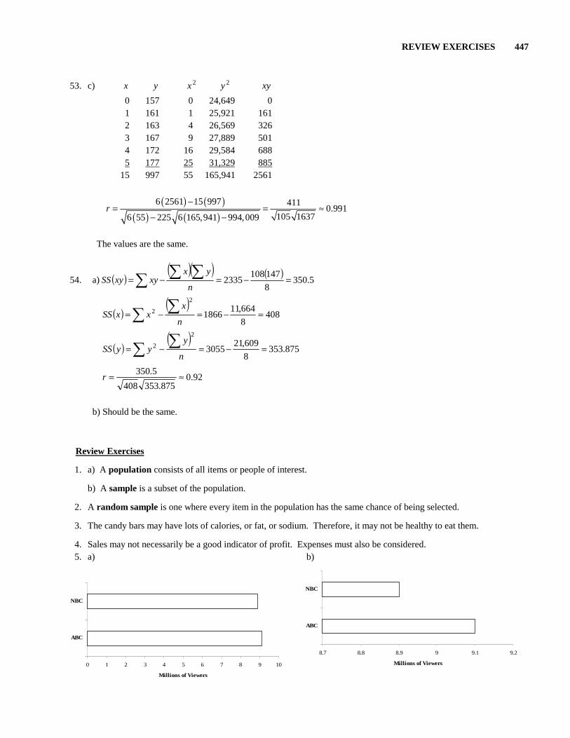
4. Sales may not necessarily be a good indicator of profit. Expenses must also be considered. 5. a)
b)
8.7 8.8 8.9 9 9.1 9.2
ABC
NBC
Millions of Viewers0 1 2 3 4 5 6 7 8 9 10
ABC
NBC
Millions of Viewers

448 CHAPTER 13 Statistics
6. a) Class Frequency b) and c) 35
36 37 38 39 40 41 42 43 44 45
1 3 6 2 3 0 4 1 3 1 1
7. a) High
Temperature Number of Cities
b) and c)
30 - 39 40 - 49 50 - 59 60 - 69 70 - 79 80 - 89
5 8 5 6 6 10
Average Daily High Temperature in January for
Selected Cities
02468
10
34.5 44.5 54.5 64.5 74.5 84.5
Average Daily High Temperature
Num
ber
of C
itie
s
d) 3 6 represents 36 3 0 3 4 5 6 4 1 2 2 3 4 7 8 8 5 0 4 4 5 6 6 5 6 6 7 8 9 7 3 5 5 7 7 9 8 0 1 3 3 4 6 6 7 8 9
8. 806
480 ==x 9. 812
8379 =+
10. None 11. 78
2
9363 =+
12. 93 − 63 = 30 13. x xx − ( )2xx −
63 -17 289 76 -4 16 79 -1 1 83 3 9 86 6 36 93 13 169 0 520
20.10104,1045
520 ≈== s
0
1
2
3
4
5
6
35 36 37 38 39 40 41 42 43 44 45
Class
Freq
uen
cy

REVIEW EXERCISES 449
14. 1312
156 ==x 15. 132
1412 =+
16. 12 and 7 17. 5.13
2
234 =+
18. 23 − 4 = 19 19. x xx − ( )2xx −
4 -9 81 5 -8 64 7 -6 36 7 -6 36 12 -1 1 12 -1 1 14 1 1 15 2 4 17 4 16 19 6 36 21 8 64 23 10 100 0 440
32.640,4011
440 ≈== s
20. 00.15
5
5
423737 −=−=−=z
00.15
5
5
424747 ==−=z
%2.68682.0341.0341.0 ==+
21. 00.25
10
5
423232 −=−=−=z
00.25
10
5
425252 ==−=z
%4.95954.0477.0477.0 ==+
22. 60.15
8
5
425050 ==−=z
%5.94945.0445.0500.0 ==+
23. 60.15
8
5
425050 ==−=z
%5.5055.0445.0500.0 ==−
24. 60.5
3
5
423939 −=−=−=z
%6.72726.0226.0500.0 ==+
25. 20
20 20 00
5 5z
−= = =
25
25 20 51.00
5 5z
−= = =
%1.34341.0 =
26. 18
18 20 20.40
5 5z
− −= = = −
%5.34345.0155.0500.0 ==−
27. 22
22 20 20.40
5 5z
−= = =
28
28 20 81.60
5 5z
−= = =
0.445 0.155 0.29 29.0%− = =
28. 30
30 20 102.00
5 5z
−= = =
0.500 – 0.477 = 0.023 = 2.3%

450 CHAPTER 13 Statistics
29. a) b) Yes; positive because generally as the year increases, the sales increase.
c) x y 2x 2y xy
0 3.9 0 15.21 0 1 3.9 1 15.21 3.9 2 4.1 4 16.81 8.2 3 4.6 9 21.16 13.8 4 4.8 16 23.04 19.2 5 4.9 25 24.01 24.5 15 26.2 55 115.44 69.6
( ) ( )
( ) ( )6 69.6 15 26.2 24.6
0.964105 6.26 55 225 6 115.44 686.44
r−
= = ≈− −
d) Yes, 0.964 0.811>
e) ( ) ( )
( )6 69.6 15 26.2 24.6
0.26 55 225 105
m−
= = ≈−
( )24.6
26.2 15105 3.8, 0.2 3.86
b y x−
= ≈ = +
30. a) b) Yes; negative because generally as the year increases, the number of owners decreases.
3.7
3.9
4.1
4.3
4.5
4.7
4.9
0 1 2 3 4 5
Year
Sale
s ($
billi
ons)
050
100150200250300350400450500550600650700750800850900
0 1 2 3 4 5
Year
Num
ber
of O
wne
rs

REVIEW EXERCISES 451
30. c) x y 2x 2y xy
0 897 0 804,609 0 1 800 1 640,000 800 2 770 4 592,900 1540 3 760 9 577,600 2280 4 735 16 540,225 2940 5 663 25 439,569 3315 15 4625 55 3,594,903 10,875
( ) ( )
( ) ( )6 10,875 15 4625 4125
0.952105 178,7936 55 225 6 3,594,903 21,390,625
r− −= = ≈ −
− −
d) Yes, 0.952 0.811− >
e) ( ) ( )
( )6 10,875 15 4625 4125
39.36 55 225 105
m− −= = ≈ −−
( )4125
4625 15105 869.0, 39.3 869.06
b y x
−−= ≈ = − +
31. a) b) Yes; negative because generally as the price increases, the number sold decreases.
c) x y 2x 2y xy
0.75 200 0.5625 40,000 150 1.00 160 1 25,600 160 1.25 140 1.5625 19,600 175 1.50 120 2.25 14,400 180 1.75 110 3.0625 12,100 192.5 2.00 95 4 9025 190 8.25 825 12.4375 120,725 1047.5
( ) ( )
( ) ( )6 1047.5 8.25 825 521.25
0.9736.5625 43,7256 12.4375 68.0625 6 120,725 680,625
r− −= = ≈ −
− −
d) Yes, 0.973 0.811− >
0
50
100
150
200
0.00 0.25 0.50 0.75 1.00 1.25 1.50 1.75 2.00
Price (dollars)
Num
ber
Sold

452 CHAPTER 13 Statistics
31. e) ( ) ( )( )
6 1047.5 8.25 825 521.2579.4
6 12.4375 68.0625 6.5625m
− −= = ≈ −−
( )521.25
825 8.256.5625 246.7, 79.4 246.7
6b y x
−−= ≈ = − +
f) ( )79.4 1.60 246.7 119.66 120 soldy = − + = ≈
32. Mode = 175 lb 33. Median = 180 lb 34. 25% 35. 25% 36 100% - 86% = 14% 37. 100(187) = 18,700 lb 38. 187 + 2(23) = 233 lb 39. 187 - 1.8(23) = 145.6 lb
40. 150
3.5742
x = ≈ 41. 2
42. 3 3
32
+ = 43. 72
140 =+
44. 14 - 0 = 14
45. x xx − ( )2xx − x xx − ( )2xx − x xx − ( )2xx −
0 -3.6 12.96 2 -1.6 2.56 4 0.4 0.16 0 -3.6 12.96 2 -1.6 2.56 5 1.4 1.96 0 -3.6 12.96 3 -0.6 0.36 5 1.4 1.96 0 -3.6 12.96 3 -0.6 0.36 5 1.4 1.96 0 -3.6 12.96 3 -0.6 0.36 6 2.4 5.76 0 -3.6 12.96 3 -0.6 0.36 6 2.4 5.76 1 -2.6 6.76 3 -0.6 0.36 6 2.4 5.76 1 -2.6 6.76 3 -0.6 0.36 6 2.4 5.76 2 -1.6 2.56 4 0.4 0.16 6 2.4 5.76 2 -1.6 2.56 4 0.4 0.16 7 3.4 11.56 2 -1.6 2.56 4 0.4 0.16 8 4.4 19.36 2 -1.6 2.56 4 0.4 0.16 10 6.4 40.96 2 -1.6 2.56 4 0.4 0.16 14 10.4 108.16 2 -1.6 2.56 4 0.4 0.16 332.32 2 -1.6 2.56
332.32
8.105, 8.105 2.8541
s≈ = ≈
46. # of Child. # of Presidents 47. and 48. 0 - 1
2 - 3 4 - 5 6 - 7 8 - 9 10 - 11 12 - 13 14 - 15
8 15 10 6 1 1 0 1
Number of Children of U.S. Presidents
02468
101214161820
0.5 2.5 4.5 6.5 8.5 10.5 12.5 14.5
Number of Children
Num
ber
of P
resi
dent
s

CHAPTER TEST 453
49. No, it is skewed to the right. 50. No, some families have no children, more have one child, the greatest percent may have two children, fewer have
three children, etc. 51. No, the number of children per family has decreased over the years. Chapter Test
1. 180
365
x = = 2. 37
3. 37 4.
21 4633.5
2
+ =
5. 46 – 21 = 25 6. x xx − ( )2xx −
21 -15 225 37 1 1 37 1 1 39 3 9 46 10 100 0 336
17.984,844
336 ≈== s
7. Class Frequency 8. and 9. 25 - 30
31 - 36 37 - 42 43 - 48 49 - 54 55 - 60 61 - 66
7 5 1 7 5 3 2
0
1
2
3
4
5
6
7
27.5 33.5 39.5 45.5 51.5 57.5 63.5
Class
Fre
quen
cy
10. Mode = $695 11. Median = $670
12. 100% - 25% = 75% 13. 79%
14. 100(700) = $70,000 15. $700 + 1($40) = $740
16. $700 - 1.5($40) = $640
17. 08.2000,12
000,25
000,12
000,75000,50000,50 −≈−=−=z
70,000
70,000 75,000 50000.42
12,000 12,000z
− −= = ≈ −
%8.31318.0163.0481.0 ==−
18. 25.1000,12
000,15
000,12
000,75000,60000,60 −=−=−=z
%4.89894.0394.0500.0 ==+
19. 25.1000,12
000,15
000,12
000,75000,90000,90 ==−=z
%6.10106.0394.0500.0 ==−

454 CHAPTER 13 Statistics
20. From #17 and #18, 25.1000,60 −=z and 70,000 0.42z ≈ −
%1.23231.0163.0394.0 ==− ( ) 693.69300231.0 ≈= cars
21. a) b) Yes
c) x y 2x 2y xy
0 9.8 0 96.04 0 10 11.3 100 127.69 113 20 12.5 400 156.25 250 25 12.8 625 163.84 320 30 12.4 900 153.76 372 85 58.8 2025 697.58 1055
( ) ( )
( ) ( )5 1055 85 58.8 277
0.9322900 30.465 2025 7225 5 697.58 3457.44
r−
= = ≈− −
d) Yes, 0.932 0.878>
e) ( ) ( )
( )5 1055 85 58.8 277
0.15 2025 7225 2900
m−
= = ≈−
( )277
58.8 852900 10.1, 0.1 10.15
b y x−
= ≈ = +
f) ( )0.1 40 10.1 14.1%y = + =
Group Projects
1. a) – j) Answers will vary. 2. a) – g) Answers will vary.
0
2
4
6
8
10
12
14
0 10 20 30 40
Year
Per
cen
t
y
x