chapter 10 making capital investment decisions 10.1project cash flows: a first look 10.2incremental...

Chapter 10 Making Capital Investment Decisions

10.1 Project Cash Flows: A First Look

10.2 Incremental Cash Flows

10.3 Pro Forma Financial Statements and Project Cash Flows

10.4 More on Project Cash Flows

10.5 Alternative Definitions of Operating Cash Flow

10.6 Some Special Cases of Discounted Cash Flow Analysis

10.7 Summary and Conclusions

Vigdis Boasson Mgf301, School of Management, SUNY at Buffalo

Vigdis Boasson Mgf 301, School of Management, SUNY at Buffalo

10.2 Fundamental Principles of Project Evaluation

Fundamental Principles of Project Evaluation:

Project evaluation - the application of one or more capital budgeting decision rules to estimated relevant project cash flows in order to make the investment decision.

Relevant cash flows - the incremental cash flows associated with the decision to invest in a project.

The incremental cash flows - any and all changes in the firm’s future cash flows that are a direct consequence of taking the project.

Stand-alone principle - evaluation of a project based on the project’s incremental cash flows.



Incremental Cash Flows

We are concerned only with those cash flows that are incremental and that result from a project.

Incremental cash flows Do Not include: Sunk costs Opportunity costs Side Effects Net working capital Financing costs



Non-Incremental Cash Flows: Sunk costs :A cost that has already been incurred and cannot be

removed. Opportunity costs: Any cash flows lost or foregone by taking one

course of action rather than another. Side effects: Erosion: New project revenues gained at the expense

of existing products /services. Net working capital: New projects often require incremental

investments in cash, inventories, and receivables that need to be included in cash flows if they are not offset by changes in payables. Later, as projects end, this investment is often recovered.

Financing costs: Cash flows associated with interest payments or principal on debt, dividends. Financing costs are reflected in the discount rate used to discount the project cash flows.

Other issues: Use After-tax cash flows.


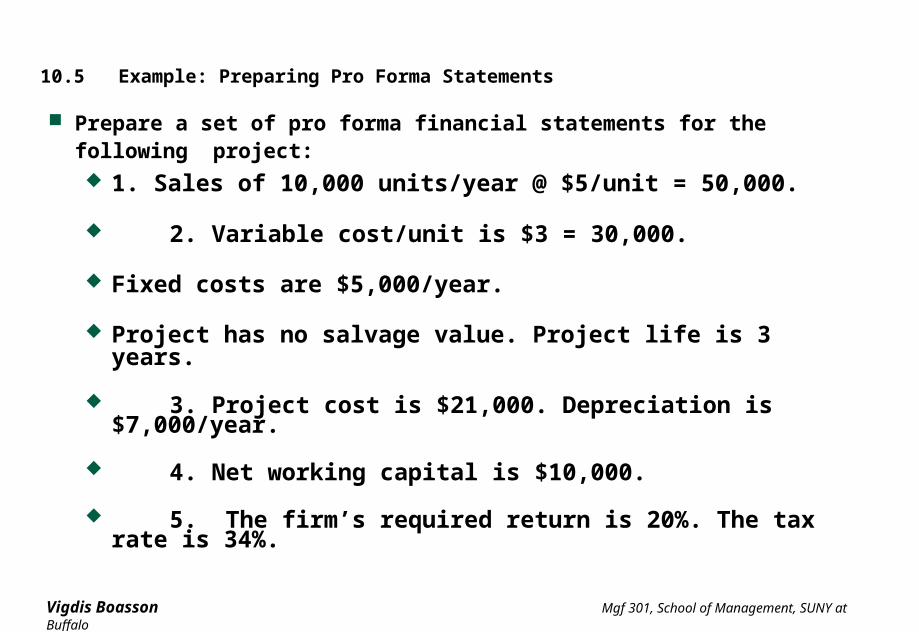
10.5 Example: Preparing Pro Forma Statements

Prepare a set of pro forma financial statements for the following project: 1. Sales of 10,000 units/year @ $5/unit = 50,000.

2. Variable cost/unit is $3 = 30,000.

Fixed costs are $5,000/year.

Project has no salvage value. Project life is 3 years.

3. Project cost is $21,000. Depreciation is $7,000/year.

4. Net working capital is $10,000.

5. The firm’s required return is 20%. The tax rate is 34%.


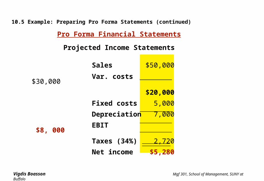
10.5 Example: Preparing Pro Forma Statements (continued)

Pro Forma Financial Statements

Projected Income Statements

Sales $50,000

Var. costs $30,000

$20,000

Fixed costs 5,000

Depreciation 7,000

EBIT $8, 000

Taxes (34%) 2,720

Net income $5,280


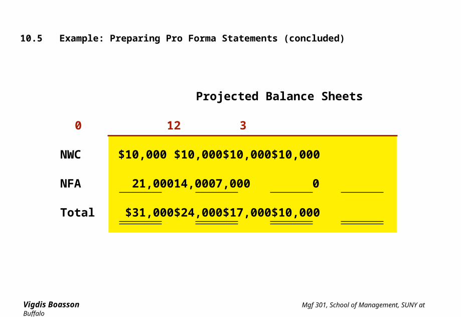
10.5 Example: Preparing Pro Forma Statements (concluded)

Projected Balance Sheets

0 1 2 3

NWC $10,000 $10,000 $10,000 $10,000

NFA 21,000 14,000 7,000 0

Total $31,000 $24,000 $17,000 $10,000


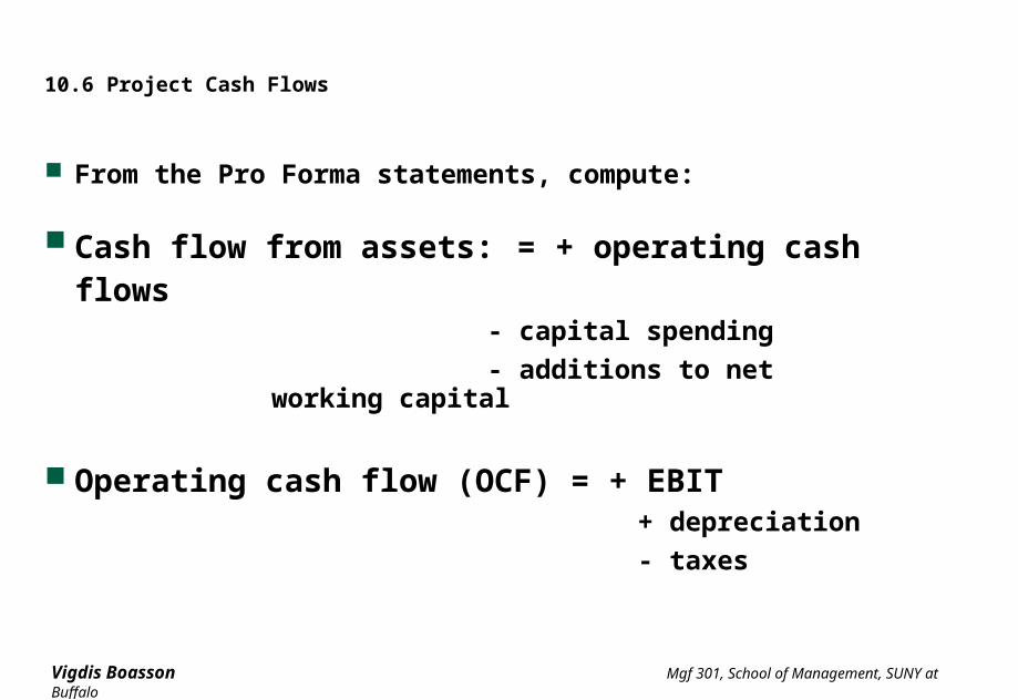
10.6 Project Cash Flows

From the Pro Forma statements, compute:

Cash flow from assets: = + operating cash flows - capital spending

- additions to net working capital

Operating cash flow (OCF) = + EBIT +

depreciation

- taxes


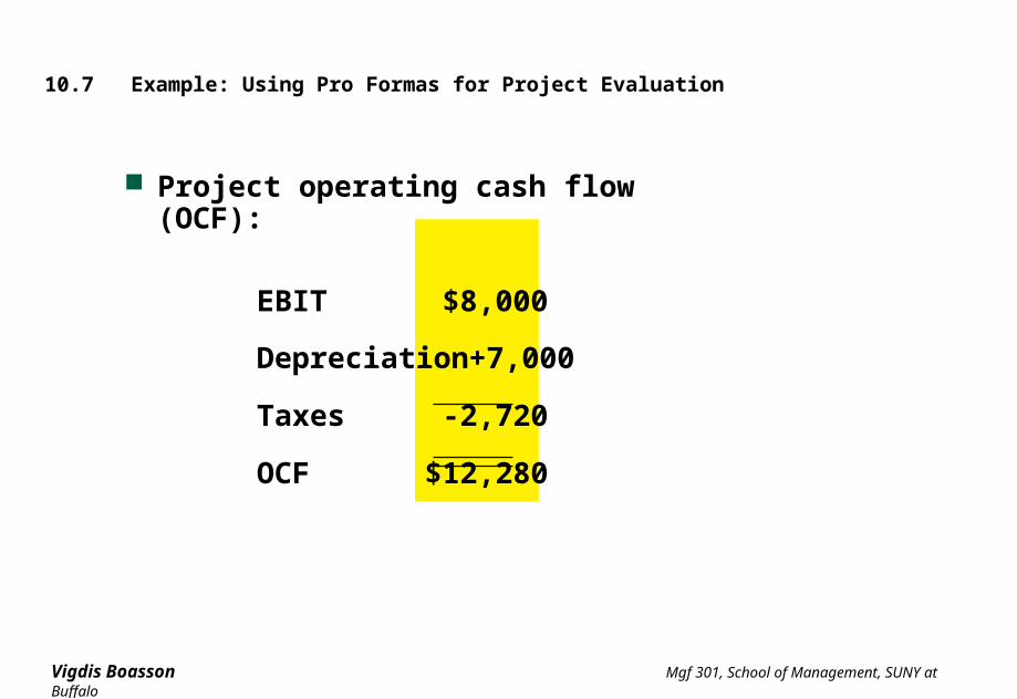
10.7 Example: Using Pro Formas for Project Evaluation

Project operating cash flow (OCF):

EBIT $8,000

Depreciation +7,000

Taxes -2,720

OCF $12,280


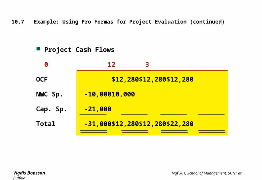
10.7 Example: Using Pro Formas for Project Evaluation (continued)

Project Cash Flows

0 1 2 3

OCF $12,280 $12,280 $12,280

NWC Sp. -10,000 10,000

Cap. Sp. -21,000

Total -31,000 $12,280 $12,280 $22,280


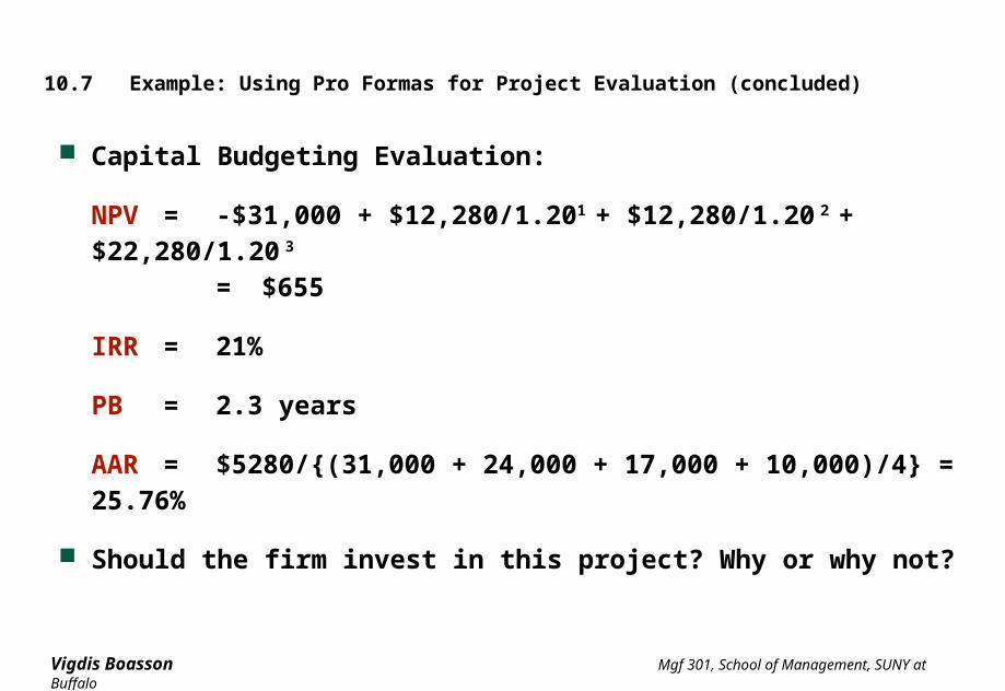
10.7 Example: Using Pro Formas for Project Evaluation (concluded)

Capital Budgeting Evaluation:

NPV = -$31,000 + $12,280/1.201 + $12,280/1.20 2 + $22,280/1.20

3

= $655

IRR = 21%

PB = 2.3 years

AAR = $5280/{(31,000 + 24,000 + 17,000 + 10,000)/4} = 25.76%

Should the firm invest in this project? Why or why not?


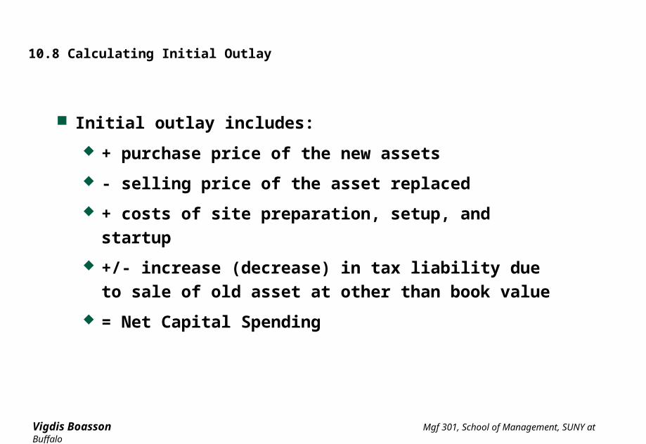
10.8 Calculating Initial Outlay

Initial outlay includes:

+ purchase price of the new assets

- selling price of the asset replaced

+ costs of site preparation, setup, and startup

+/- increase (decrease) in tax liability due to sale of old

asset at other than book value

= Net Capital Spending


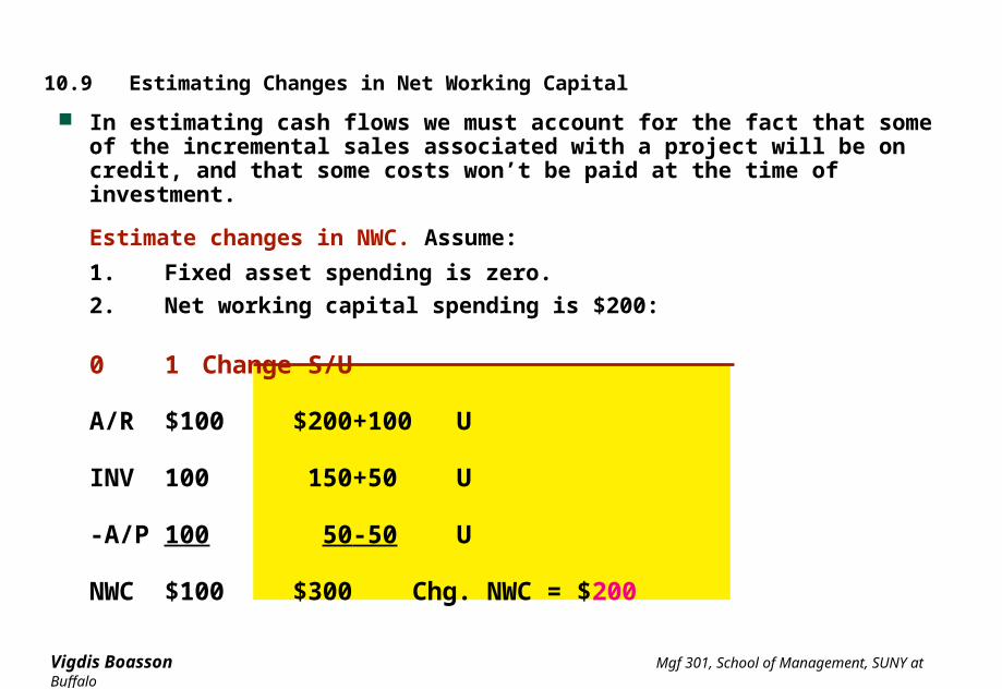
10.9 Estimating Changes in Net Working Capital

In estimating cash flows we must account for the fact that some of the incremental sales associated with a project will be on credit, and that some costs won’t be paid at the time of investment.

Estimate changes in NWC. Assume:

1. Fixed asset spending is zero.

2. Net working capital spending is $200:

0 1 Change S/U

A/R $100 $200 +100 U

INV 100 150 +50 U

-A/P 100 50 -50 U

NWC $100 $300 Chg. NWC = $200


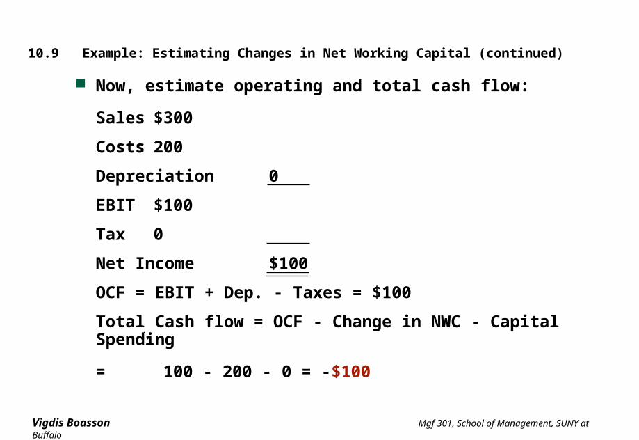
10.9 Example: Estimating Changes in Net Working Capital (continued)

Now, estimate operating and total cash flow:

Sales $300

Costs 200

Depreciation 0

EBIT $100

Tax 0

Net Income $100

OCF = EBIT + Dep. - Taxes = $100

Total Cash flow = OCF - Change in NWC - Capital Spending

= 100 - 200 - 0 = -$100


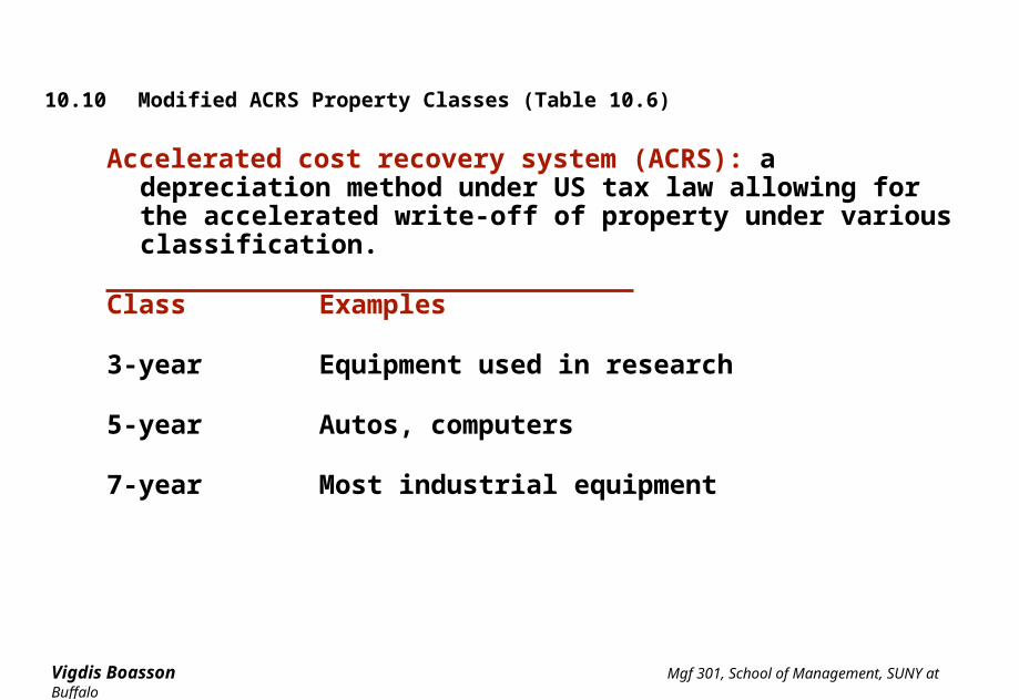
10.10 Modified ACRS Property Classes (Table 10.6)

Accelerated cost recovery system (ACRS): a depreciation method under US tax law allowing for the accelerated write-off of property under various classification.

Class Examples

3-year Equipment used in research

5-year Autos, computers

7-year Most industrial equipment


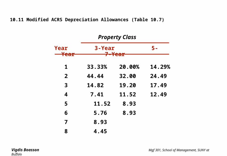
10.11 Modified ACRS Depreciation Allowances (Table 10.7)

Property Class

Year 3-Year 5-Year 7-Year

1 33.33% 20.00%14.29%

2 44.44 32.00 24.49

3 14.82 19.20 17.49

4 7.41 11.52 12.49

5 11.52 8.93

6 5.76 8.93

7 8.93

8 4.45


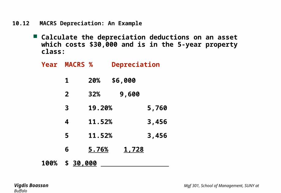
10.12 MACRS Depreciation: An Example

Calculate the depreciation deductions on an asset which costs $30,000 and is in the 5-year property class:

Year MACRS % Depreciation

1 20% $6,000

2 32% 9,600

3 19.20% 5,760

4 11.52% 3,456

5 11.52% 3,456

6 5.76% 1,728

100% $ 30,000


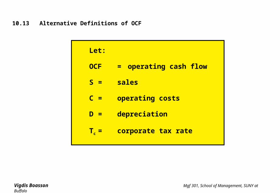
10.13 Alternative Definitions of OCF

Let:

OCF = operating cash flow

S = sales

C = operating costs

D = depreciation

Tc = corporate tax rate


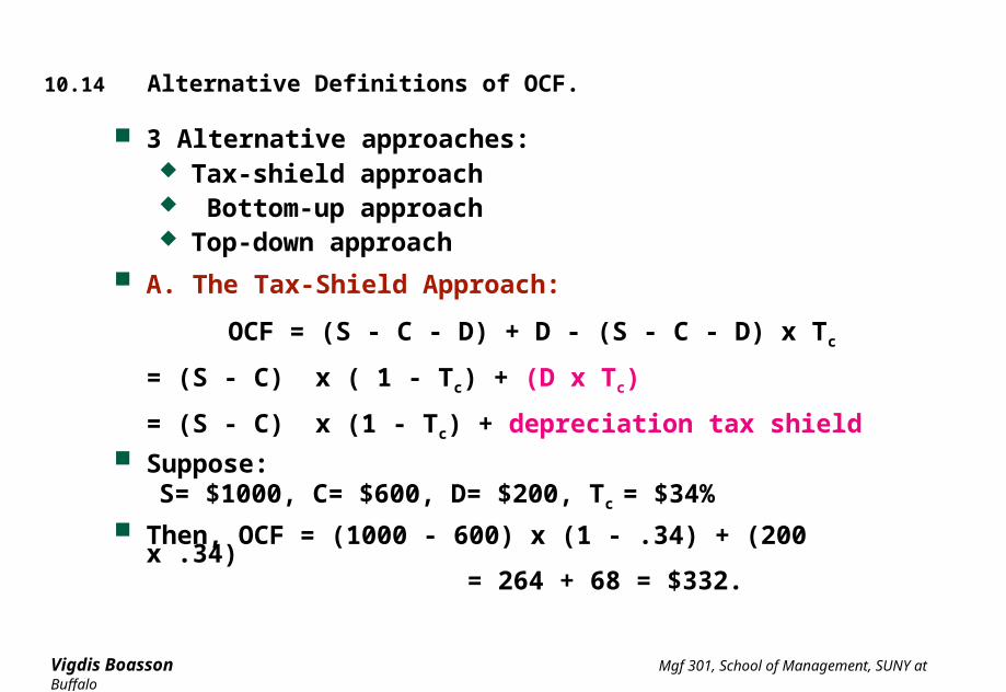
10.14 Alternative Definitions of OCF.

3 Alternative approaches: Tax-shield approach Bottom-up approach Top-down approach

A. The Tax-Shield Approach:

OCF = (S - C - D) + D - (S - C - D) x Tc

= (S - C) x ( 1 - Tc) + (D x Tc)

= (S - C) x (1 - Tc) + depreciation tax shield Suppose:

S= $1000, C= $600, D= $200, Tc = $34% Then, OCF = (1000 - 600) x (1 - .34) + (200 x .34)

= 264 + 68 = $332.


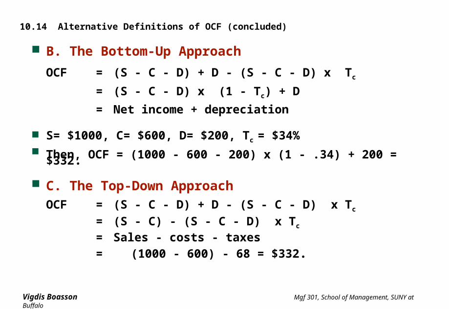
10.14 Alternative Definitions of OCF (concluded)

B. The Bottom-Up Approach

OCF = (S - C - D) + D - (S - C - D) x Tc

= (S - C - D) x (1 - Tc) + D

= Net income + depreciation

S= $1000, C= $600, D= $200, Tc = $34% Then, OCF = (1000 - 600 - 200) x (1 - .34) + 200 = $332.

C. The Top-Down Approach

OCF = (S - C - D) + D - (S - C - D) x Tc

= (S - C) - (S - C - D) x Tc

= Sales - costs - taxes

= (1000 - 600) - 68 = $332.


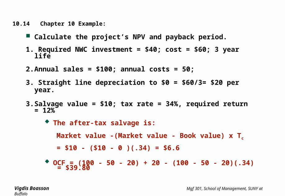
10.14 Chapter 10 Example:

Calculate the project’s NPV and payback period.

1. Required NWC investment = $40; cost = $60; 3 year life

2. Annual sales = $100; annual costs = 50;

3. Straight line depreciation to $0 = $60/3= $20 per year.

3. Salvage value = $10; tax rate = 34%, required return = 12%

The after-tax salvage is:

Market value -(Market value - Book value) x Tc

= $10 - ($10 - 0 )(.34) = $6.6

OCF = (100 - 50 - 20) + 20 - (100 - 50 - 20)(.34) = $39.80


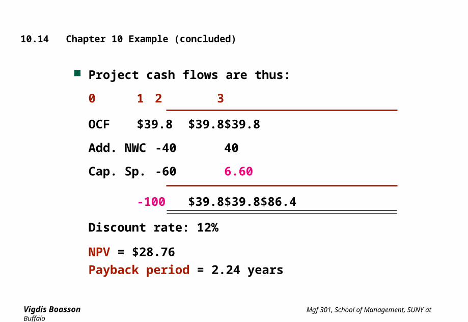
10.14 Chapter 10 Example (concluded)

Project cash flows are thus:

0 1 2 3

OCF $39.8 $39.8 $39.8

Add. NWC -40 40

Cap. Sp. -60 6.60

-100 $39.8 $39.8 $86.4

Discount rate: 12%

NPV = $28.76

Payback period = 2.24 years


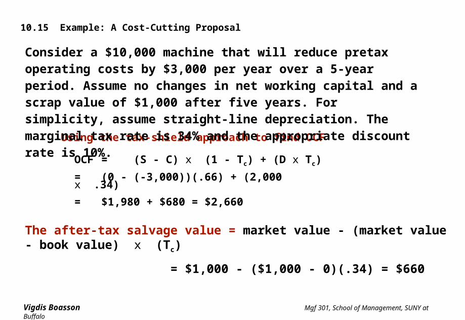
10.15 Example: A Cost-Cutting Proposal

Using the tax-shield approach to find OCF

OCF = (S - C) x (1 - Tc) + (D x Tc)

= (0 - (-3,000))(.66) + (2,000 x .34)

= $1,980 + $680 = $2,660

The after-tax salvage value = market value - (market value - book value) x (Tc)

= $1,000 - ($1,000 - 0)(.34) = $660

Consider a $10,000 machine that will reduce pretax operating costs by $3,000 per year over a 5-year period. Assume no changes in net working capital and a scrap value of $1,000 after five years. For simplicity, assume straight-line depreciation. The marginal tax rate is 34% and the appropriate discount rate is 10%.


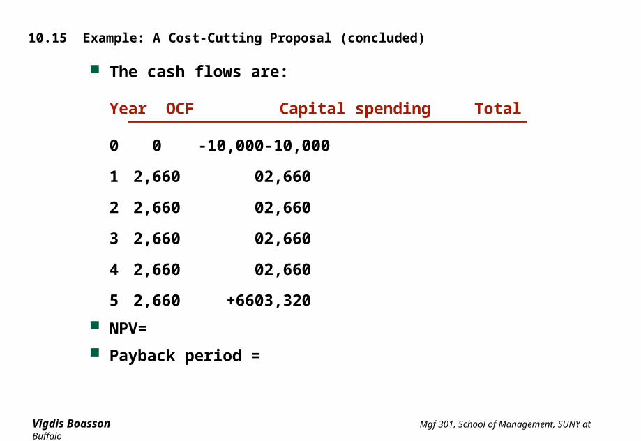
10.15 Example: A Cost-Cutting Proposal (concluded)

The cash flows are:

Year OCF Capital spending Total

0 0 -10,000 -10,000

1 2,660 0 2,660

2 2,660 0 2,660

3 2,660 0 2,660

4 2,660 0 2,660

5 2,660 +660 3,320

NPV=

Payback period =

chapter 10 making capital investment decisions 10.1project cash flows: a first look 10.2incremental...

Documents