chapter 1

Automatic control theory

A Course ——used for analyzing and designing a automatic control system

Chapter 1 Introduction

M

Water pool

val ve

fl oat

ampl i fi er

motor

Gearassembl y

+

-

Figure 1.1

* Operating principle……

* Feedback control……

1) A water-level control system

21 century — information age, cybernetics(control theory), system approach and information theory , three science theory mainstay(supports) in 21 century.

1.1 Automatic control A machine(or system) work by machine-self, not by manual operation.

1.2 Automatic control systems

1.2.1 examples


Water exi t

waterentrance

fl oat

l ever

Fi gure 1.2

* Operating principle……* Feedback control……

2) A temperature Control system (shown in Fig.1.3)

M

+

e

ua=k(ur-uf)

ur

uf

ampl i fi er

thermometer

Gearassembl y

contai ner

Fi gure 1.3

* Operating principle…

* Feedback control(error)…

Another example of the water-level

control is shown in figure 1.2.


3) A DC-Motor control system

M

M

+

-

+

regul atortri gger

recti fi er

DCmotor

techometer

l oad

e

Uf (Feedback)

ur

Fi g. 1.4

ua

Uk=k(ur-uf)

* Principle…

* Feedback control(error)…


4) A servo (following) control system

servopotenti ometer

M

+

-

InputT r

outputT c

servomechani sm

servo motorservomodul ator

l oad

* principle……

* feedback(error)……

Fig. 1.5


* principle……

* feedback(error)……

government(Fami l y pl anni ng commi ttee)

census

soci ety

excessprocreate

Desi re popul ati on popul ati on+

- Pol i cy orstatutes

Fig. 1.6

5) A feedback control system model of the family planning

(similar to the social, economic, and political realm(sphere or field))


x2

x3

Si gnal(vari abl e)

xxxComponents(devi ces)

+-+x1 e Adders (compari son)

e=x1+x3-x2

x

Fig. 1.7

Example:

1.2.2 block diagram of control systems The block diagram description for a control system : Convenience


amplifier Motor Gearing Valve

Actuator

Watercontainer

Processcontroller

Float

measurement (Sensor)

Error

Feedback signal

resistance comparator

Desired water level

Input

Actual water level

Output

Fig. 1.8

For the Fig.1.1, The water level control system:

M

Water pool

val ve

fl oat

ampl i fi er

motor

Gearassembl y

+

-

Figure 1.1


For the Fig. 1.4, The DC-Motor control system

Desi red rotate speed n

Regul ator Tri gger Recti fi er DCmotor

Techometer

Actuator

Processcontrol l er

measurement (Sensor)

comparator

Actual rotate speed n

Error

Feedback si gnal

Referencei nput ur

Output n

Fi g. 1.9

auk ua

uf

e


1.2.3 Fundamental structure of control systems

1) Open loop control systems

Control l er Actuator Process

Di sturbance(Noi se)

Input r(t)

Reference desi red output

Output c(t)(actual output)

Controlsi gnal

Actuati ngsi gnal

uk uact

Fi g. 1.10

Features: Only there is a forward action from the input to the output.


2) Closed loop (feedback) control systems

Control l er Actuator Process

Di sturbance(Noi se)

Input r(t)

Reference desi red output

Output c(t)(actual output)

Controlsi gnal

Actuati ngsi gnal

uk uact

Fi g. 1.11

measurementFeedback si gnal b(t)

+-

(+)

e(t)=r(t)-b(t)

Features:

1) measuring the output (controlled variable) . 2) Feedback.

not only there is a forward action , also a backward action between the output and the input (measuring the output and comparing it with the input).

Chapter 1 Introduction Notes: 1) Positive feedback; 2) Negative feedback—Feedback.1.3 types of control systems

1) linear systems versus Nonlinear systems.

2) Time-invariant systems vs. Time-varying systems.

3) Continuous systems vs. Discrete (data) systems.

4) Constant input modulation vs. Servo control systems.

1.4 Basic performance requirements of control systems

1) Stability.

2) Accuracy (steady state performance).

3) Rapidness (instantaneous characteristic).


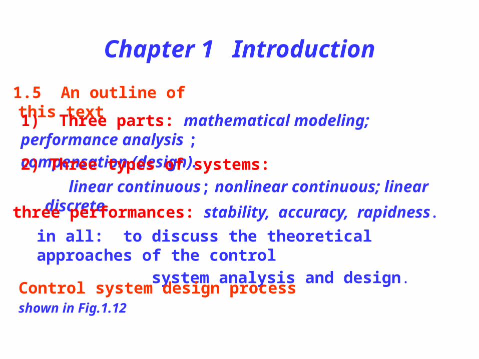
1.5 An outline of this text

1) Three parts: mathematical modeling; performance analysis ;

compensation (design). 2) Three types of systems:

linear continuous; nonlinear continuous; linear discrete.

3) three performances: stability, accuracy, rapidness.

in all: to discuss the theoretical approaches of the control

system analysis and design.

1.6 Control system design process shown in Fig.1.12


1. Establish control goals

2. Identify the variables to control

3. Write the specifications for the variables

4. Establish the system configuration Identify the actuator

5. Obtain a model of the process, the actuator and the sensor

6. Describe a controller and select key parameters to be adjusted

7. Optimize the parameters and analyze the performance

Performance does not Meet the specifications

Finalize the design

Performance meet the specifications

Fig.1.12

Chapter 1 Introduction1.7 Sequential design example: disk drive read system

Actuator motor

Arm

SpindleTrack a

Track b

Head slider

Rotation of arm Disk

Fig.1.13 A disk drive read system

A disk drive read system Shown in Fig.1.13

◆ Configuration◆ Principle 　

Chapter 1 IntroductionSequential design:

here we are concerned with the design steps 1,2,3, and 4 of Fig.1.12.

(1) Identify the control goal:

(2) Identify the variables to control:

Position the reader head to read the date stored on a track on the disk.

the position of the read head.

(3) Write the initial specification for the variables:

The disk rotates at a speed of between 1800 and 7200 rpm and the read head “flies” above the disk at a distance of less than 100 nm. The initial specification for the position accuracy to be controlled:≤ 1 μm (leas than 1 μm ) and to be able to move the head from track a to track b within 50 ms, if possible.

Chapter 1 Introduction(4) Establish an initial system configuration:

It is obvious : we should propose a closed loop system , not a open loop system.

An initial system configuration can be shown as in Fig.1.13.

Control device

Actuator motor

Read arm

sensor

Desired head position

error Actual head position

Fig.1.13 system configuration for disk drive

We will consider the design of the disk drive further in the after-mentioned chapters.

Chapter 1 IntroductionExercise: E1.6, P1.3, P1.13

Chapter 2 mathematical models of systems2.1 Introduction

Controller Actuator Process

Disturbance

Input r(t)

desired output temperature

Output T(t)

actual output temperature

Controlsignal

Actuatingsignal

uk uac

Fig. 2.1

temperature measurement

Feedback signal b(t)

+-( － )

e(t)=r(t)-b(t)

1) Easy to discuss the full possible types of the control systems—in terms of the system’s “mathematical characteristics”. 2) The basis — analyzing or designing the control systems.

For example, we design a temperature Control system :

The key — designing the controller → how produce uk.

2.1.1 Why ？

Chapter 2 mathematical models of systems

2.1.3 How get ？ 1) theoretical approaches 2) experimental approaches

3) discrimination learning

2.1.2 What is ？ Mathematical models of the control systems—— the mathematical relationships between the system’s variables.

Different characteristic of the process — different uk:

T(t)

uk

T1

T2

uk12uk11

uk21

Ⅰ

Ⅱ For T1

12

11

k

k

u

u

Ⅱ

Ⅰ

For T1

22

21

k

k

u

u

Ⅱ

Ⅰ


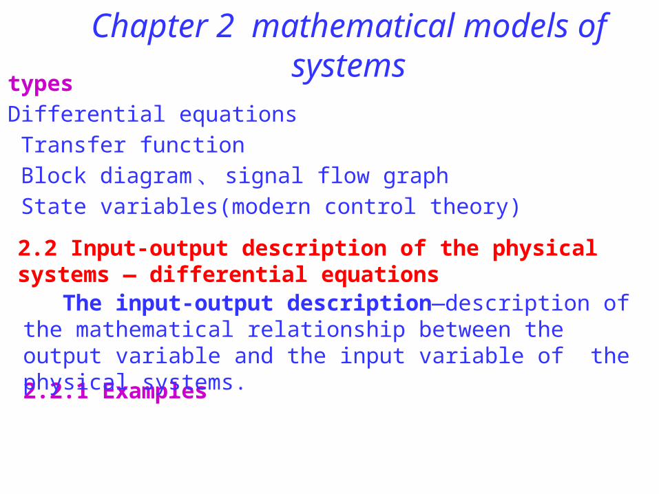
2.2.1 Examples

2.2 Input-output description of the physical systems — differential equations

2.1.4 types

1) Differential equations

2) Transfer function

3) Block diagram 、 signal flow graph

4) State variables(modern control theory)

The input-output description—description of the mathematical relationship between the output variable and the input variable of the physical systems.


ur uc

R L

Ci

define: input → ur output → uc 。

we have ：

rccc

crc

uudt

duRC

dt

udLC

dt

duCiuu

dt

diLRi

2

2

rccc uu

dt

duT

dt

udTTT

R

LTRCmake 12

2

2121:

Example 2.1 : A passive circuit

Chapter 2 mathematical models of systemsExample 2.2 : A mechanism

y

k

f

F

m

Define: input → F ， output → y. We have:

Fkydt

dyf

dt

ydm

td

ydm

dt

dyfkyF

2

2

2

2

Fk

ydt

dyT

dt

ydTThavewe

Tf

mT

k

fmakeweIf

1:

:

12

2

21

2,1

Compare with example 2.1: uc→y; ur→F ─ analogous systems

Chapter 2 mathematical models of systems Example 2.3 : An operational amplifier (Op-amp) circuit

uruc

R1

C

R2

R4

R1

R3

i 3

i 1

i 2

+-

Input →ur output →uc

)3........(....................).........(1

)2...(........................................

)1)......(()(1

223

3

112

2342333

iRuR

i

R

uii

iiRdtiiC

iRu

c

r

c

(2)→(3); (2)→(1); (3)→(1) ：

r

rCRRR

RR

RRR

ccCR u

dt

duu

dt

du)( 4

32

324

1

32

)(:

)(;;: 432

32

1

324

rr

cc u

dt

duku

dt

duThavewe

CRRR

RRk

R

RRTCRmake

Chapter 2 mathematical models of systems Example 2.4 : A DC motor

ua

w1

RaLa

i aM

w3

w2 (J 3, f3)

(J 1, f1)

(J 2, f2)

Mf

i 1

i 2Input → ua ， output → ω1

)4.....(

)3.....(....................

)2.....(....................

)1....(

11

1

fdt

dJMM

CE

iCM

uEiRdt

diL

ea

am

aaaaa

a

(4)→(2)→(1) and (3)→(1):

MCC

RM

CC

Lu

C

CC

fR

CC

JR

CC

fL

CC

JL

me

a

me

aa

e

me

a

me

a

me

a

me

a

1

)1()( 111


): (

..........................

......

......

:

321211

21

22

21

321

21

22

21

321

21

iiifromderivedbecan

torqueequivalentii

MM

nt coefficie frictionequivalentii

f

i

fff

inertia of momentequivalentii

J

i

JJJ

here

f

Make:

constant-timeelectricfrictionCC

fRT

constant-timeelectric-mechanicalCC

JRT

constanttimemagnetic-electricR

LT

me

af

me

am

a

ae

-.......

.......

............


ae

mme uCdt

dT

dt

dTT

12

2

Assume the motor idle: Mf = 0, and neglect the friction: f = 0, we have:

)(11

)1()( 111

MTMTTJ

uC

TTTTTT

mmeae

fmfeme

The differential equation description of the DC motor is:

Chapter 2 mathematical models of systemsExample 2.5 : A DC-Motor control system

+

tri ggerUf

ur -M

M

+

-recti fi er

DCmotor

techometer

l oad

ua-uk

R3

R1

R1

R2 R3

w

Input → ur ， Output → ω; neglect the friction:

(4)MTMTTJ

uCdt

dT

dt

dTT

(3)uku(2)u

(1)uukuuR

Ru

mmeae

mme

kaf

frfrk

)......(11

...................... .....................

..................................)......()(

2

2

2

11

2

Chapter 2 mathematical models of systems（ 2 ）→（ 1 ）→（ 3 ）→（ 4 ）， we

have ：)(

1)1( 21

1212

2MMT

J

Tu

Ckkkk

dt

dT

dt

dTT e

mr

eCmme

e

2.2.2 steps to obtain the input-output description (differential equation) of control systems

1) Determine the output and input variables of the control systems.2) Write the differential equations of each system’s components in

terms of the physical laws of the components. * necessary assumption and neglect. * proper approximation.


2.2.3 General form of the input-output equation of the linear control systems—A nth-order differential equation:

mnrbrbrbrbrb

yayayayay

mmmmm

nnnnn

.........)1(1

)2(2

)1(1

)(0

)1(1

)2(2

)1(1

)(

3) dispel the intermediate(across) variables to get the input-output description which only contains the output and input variables.

4) Formalize the input-output equation to be the “standard” form:

Input variable —— on the right of the input-output equation .

Output variable —— on the left of the input-output equation.

Writing polynomial—— according to the falling-power order.

Suppose: input → r ， output → y

Chapter 2 mathematical models of systems2.3 Linearization of the nonlinear components

2.3.1 what is nonlinearity ？ The output is not linearly vary with the linear variation of the system’s (or component’s) input → nonlinear systems (or components).

2.3.2 How do the linearization ？ Suppose: y = f(r)

The Taylor series expansion about the operating point r0 is:

))(()(

)(!3

)()(

!2

)())(()()(

00)1(

0

30

0)3(

20

0)2(

00)1(

0

rrrfrf

rrrf

rrrf

rrrfrfrf

00 :)()(: rrrandrfrfymake

equationionlinearizatrrfywehave ............)(: 0'


Examples:

Example 2.6 : Elasticity equation kxxF )(

25.0;1.1;65.12:suppose 0 xpointoperatingk

11.1225.01.165.12)()( 1.00

'1' xFxkxF

equationionlinearizatxΔF

xxxFxF

..............11.12 :is that

)(11.12)()( :have we 00

Example 2.7 : Fluxograph equation

pkpQ )(

Q —— Flux; p —— pressure difference


equationionlinearizatpp

kQ

p

kpQbecause

...........2

: thus

2)(' :

0

2.4 Transfer function Another form of the input-output(external) description of control systems, different from the differential equations.

2.4.1 definition Transfer function: The ratio of the Laplace transform of the output variable to the Laplace transform of the input variable,with all initial condition assumed to be zero and for the linear systems, that is:


)(

)()(

sR

sCsG

C(s) —— Laplace transform of the output variable R(s) —— Laplace transform of the input variable G(s) —— transfer function

* Only for the linear and stationary(constant parameter) systems.* Zero initial conditions.* Dependent on the configuration and the coefficients of the systems, independent on the input and output variables.

2.4.2 How to obtain the transfer function of a system

1) If the impulse response g(t) is known

Notes:


)()( tgLsG

1)()()( if ,)(

)()( sRttr

sR

sCsG

Because:

We have:

Then:

Example 2.8 :)2(

)5(2

2

35)( 35)( 2

ss

s

sssGetg t

2) If the output response c(t) and the input r(t) are known

We have: )(

)()(

trL

tcLsG

)()()( tgLsCsG

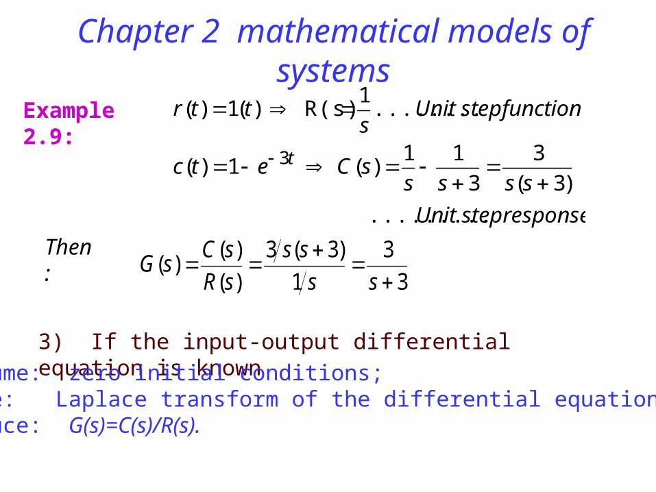
Chapter 2 mathematical models of systems Example 2.9:

responseUnit step

sssssCetc

functionUnit step s

ttr

t

.........

)3(

3

3

11)( 1)(

........1

R(s) )(1)(

3

Then:

3

3

1

)3(3

)(

)()(

ss

ss

sR

sCsG

3) If the input-output differential equation is known • Assume: zero initial conditions;• Make: Laplace transform of the differential equation;• Deduce: G(s)=C(s)/R(s).


Example 2.10:

432

65

)(6)(5)(4)(3)(2

)(6)(5)(4)(3)(2

2

2

ss

s

R(s)

C(s) G(s)

sRssRsCssCsCs

trtrtctctc

4) For a circuit

* Transform a circuit into a operator circuit.* Deduce the C(s)/R(s) in terms of the circuits theory.

Chapter 2 mathematical models of systems Example 2.11: For a electric circuit:

ucur C1 C2

R1 R2

uc(s)1/C1s 1/C2s

R1 R2

ur(s)

2112222111

r

c

r

rc

CR; TCR; TCRT

sTTTsTTsU

sUsG

sUsTTTsTT

sCR

sCsU

sCR

sCR

sCR

sCsU

:here

1)(

1

)(

)()(

)(1)(

1

1

1

)()

1(//

1

)1

(//1

)(

12212

21

12212

21

22

2

22

11

22

1

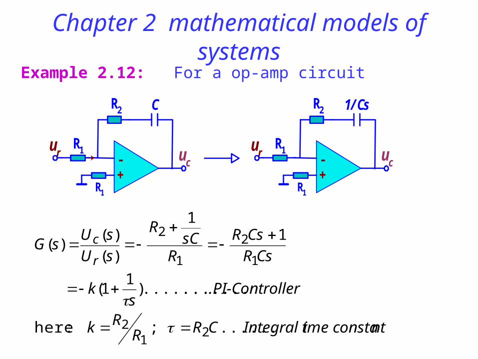
Chapter 2 mathematical models of systemsExample 2.12: For a op-amp circuit

ur uc

R1

R2

R1

+-

C R2 1/Cs

ur uc

R1

R1

+-

...... ; :here

.................)1

1(

11

)(

)()(

21

2

1

2

1

2

ntime constaIntegral tCRRRk

ller.PI-Contros

k

CsR

CsR

RsC

R

sU

sUsG

r

c


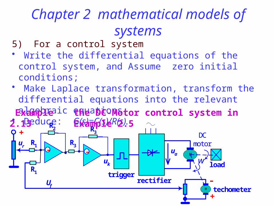
5) For a control system• Write the differential equations of the control system, and

Assume zero initial conditions;• Make Laplace transformation, transform the differential

equations into the relevant algebraic equations; • Deduce: G(s)=C(s)/R(s).

Example 2.13

+

tri ggerUf

ur -M

M

+

-recti fi er

DCmotor

techometer

l oad

ua-uk

R3

R1

R1

R2 R3

w

the DC-Motor control system in Example 2.5


In Example 2.5, we have written down the differential equations as:

(4)MMTJ

Tu

Cdt

dT

dt

dTT

(3)uku(2)u

(1)uukuuR

Ru

em

ae

mme

kaf

frfrk

)......(1

................... ....................

.........................).........()(

2

2

2

11

2

Make Laplace transformation, we have:

(4)sMJ

TsTTsU

CessTsTT

(3)sUksU(2)ssU

(1)sUsUksU

mmeamme

kaf

frk

)......()(1

)()1(

.....).........()( ......).........()(

...........................................)]........()([)(

2

2

1


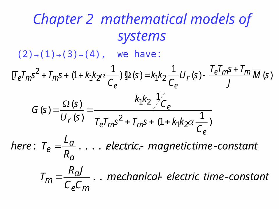
(2)→(1)→(3)→(4), we have:

)()(1

)()]1

1([ 21212 sM

J

TsTTsU

Ckks

CkksTsTT mme

ree

mme

- ......

- ........... :

constanttimeelectricmechanicalCC

JRT

constanttimemagnetic electricR

LThere

me

am

a

ae

)1

1(

1

)(

)()(

212

21

emme

e

rC

kksTsTT

Ckk

sU

ssG


2.5 Transfer function of the typical elements of linear systems

A linear system can be regarded as the composing of several typical elements, which are:

2.5.1 Proportioning elementRelationship between the input and output variables:

)()( tkrtc

Transfer function: ksR

sCsG

)(

)()(

Block diagram representation and unit step response:

R(s) C(s)k

1k

t

r(t) C(t)

t

Examples:

amplifier, gear train, tachometer…


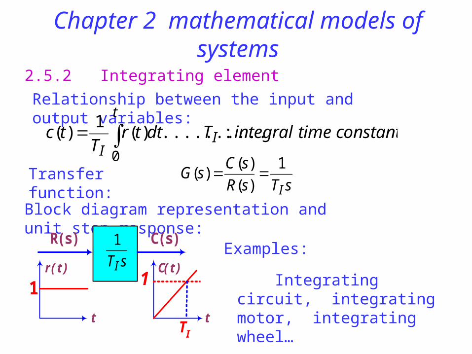
2.5.2 Integrating element

Relationship between the input and output variables:

constant timeintegralTdttrT

tc I

t

I :..........)(

1)(

0

Transfer function:sTsR

sCsG

I

1

)(

)()(


1

R(s) C(s)

1

t

r(t) C(t)

t

sTI

1

TI

Examples:

Integrating circuit, integrating motor, integrating wheel…

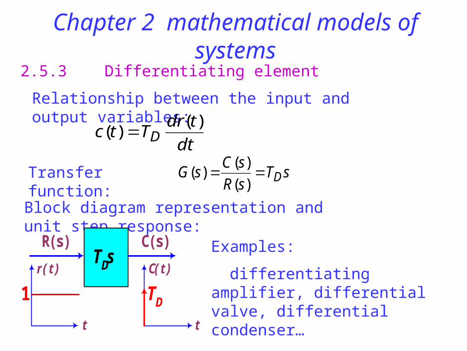
Chapter 2 mathematical models of systems2.5.3 Differentiating element


dt

tdrTtc D

)()(

Transfer function: sTsR

sCsG D

)(

)()(


Examples:

differentiating amplifier, differential valve, differential condenser…

R(s) C(s)TDs

1 TD

t

r(t) C(t)

t

2.5.4 Inertial element



)()()(

tkrtcdt

tdcT

Transfer function:1)(

)()(

Ts

k

sR

sCsG


Examples:

inertia wheel, inertial load (such as temperature system)…1

R(s) C(s)

k

t

r(t) C(t)

tT

1Ts

k

Chapter 2 mathematical models of systems2.5.5 Oscillating element


10 )()()(

2)(

2

22 tkrtc

dt

tdcT

dt

tcdT

Transfer function: 10 12)(

)()(

22

TssT

k

sR

sCsG


Examples:

oscillator, oscillating table, oscillating circuit…

R(s) C(s)12

122 TssT C(t)

k

t

1

t

r(t)

2.5.6 Delay element



)()( tkrtc

Transfer function: skesR

sCsG

)(

)()(


Examples:

gap effect of gear mechanism, threshold voltage of transistors…

R(s) C(s)

1

t

r(t)

ske

kC(t)

t

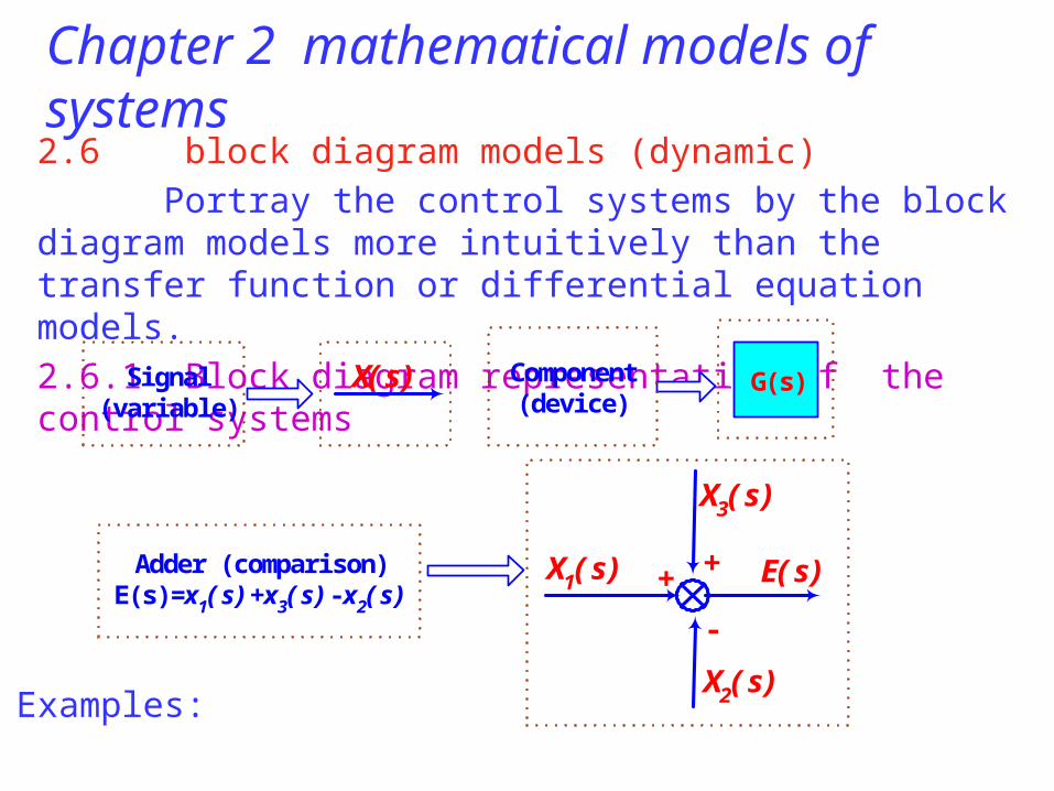
2.6 block diagram models (dynamic)

Portray the control systems by the block diagram models more intuitively than the transfer function or differential equation models.

2.6.1 Block diagram representation of the control systems


Examples:

Si gnal(vari abl e)

G(s)Component(devi ce)

Adder (compari son)E(s)=x1(s)+x3(s)-x2(s)

X(s)

X3(s)

X2(s)

+

-

+X1(s) E(s)

Example 2.14

Chapter 2 mathematical models of systemsFor the DC motor in Example 2.4

In Example 2.4, we have written down the differential equations as:

)4.....( )3.....(....................

)2.....(.................... )1....(

fdt

dJMMCE

iCMuEiRdt

diL

ea

amaaaaa

a

Make Laplace transformation, we have:

(8)sMsMfsJ

ssfssJsMsM

(7)sCsE

(6)sICsM

(5)RsL

sEsUsIsUsEsIRssIL

ea

am

aa

aaaaaaaaa

)]......()([1

)( )()()()(

..............................................................................).........()(

.............................................................................).........()(

.............)()(

)( )()()()(

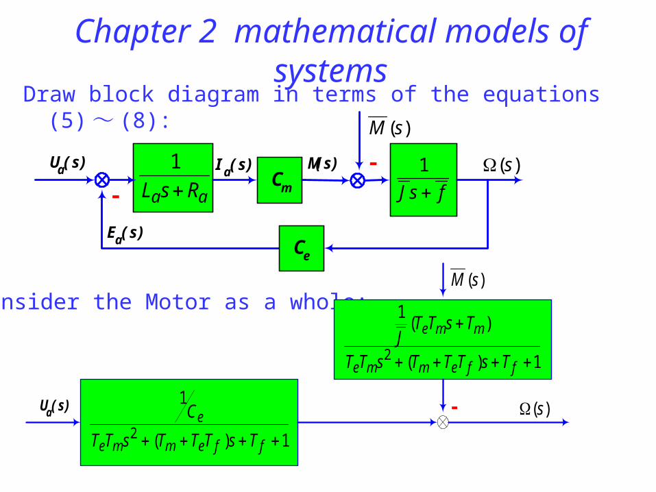
Chapter 2 mathematical models of systemsDraw block diagram in terms of the equations (5) ～ (8):

Ua(s)

aa RsL 1

Cm

Ia(s) M(s)

Ea(s)Ce

)(sfsJ

1

)(sM

-

-

Consider the Motor as a whole:

1)(

1

2 ffemme

e

TsTTTsTT

C

1)(

)(1

2

ffemme

mme

TsTTTsTT

TsTTJ

Ua(s) )(s

)(sM

-

Chapter 2 mathematical models of systemsExample 2.15 The water level control system in Fig 1.8:

Desi red water l evel

ampl i fi er Motor Geari ng Val veWater

contai ner

Fl oat

Actualwater l evel

Feedback si gnal hf

Input hi Output h

-

e ua Q

1k 1

1

2 sTsTT

C

mme

e

s

ek s2

11

3sT

k12

4

sT

k

)(1

)1(

2sM

sTsTT

sTJ

T

mme

em

Chapter 2 mathematical models of systemsThe block diagram model is:

chapter 1

Documents

control system analysis

servo control systems

temperature control

control goals2

feedback control system

waterlevel control system

water level control

control system design