channel blurring: a study of cross-retail format shopping among

1

Channel Blurring

A Study of Cross-Retail Format Shopping among US Households

Ryan Luchs1

J Jeffrey Inman

Venkatesh Shankar

January 20 2014

1Ryan Luchs is an assistant professor of marketing at the Palumbo-Donahue School of Business Duquesne

University Pittsburgh PA J Jeffrey Inman is the Albert Wesley Frey Professor of Marketing at the Katz Graduate

School of Business University of Pittsburgh Pittsburgh PA Venkatesh Shankar is Coleman Chair Professor in

Marketing at the Mays Business School Texas AampM University College Station TX Please address all

correspondence to Ryan Luchs (luchsrduqedu)Duquesne University Pittsburgh PA

2

Channel Blurring


ABSTRACT

Channel blurringmdasha phenomenon in which consumers are moving their purchases of a product

category from channels or retail formats traditionally associated with that category (eg grocery)

to alternative channels (eg mass club extreme valuedollar) and in which retailers from one

channel are selling items traditionally associated with other channelsmdashis of great interest to both

manufacturers and retailers At one time different retail formats such as grocery drug and mass

merchandiser served different purposes but they are becoming indistinguishable For example

large mass merchandisers such as Walmart are now carrying sizeable assortments of grocery

pharmaceutical and electronic products while large drug chains such as Walgreens and CVS are

stocking their shelves with toys and household items We seek to understand how consumers are

responding to these changes We develop a new measure that we call the Channel Blurring

Index which characterizes the degree of channel blurring for a household We develop a model

with the index as a function of demographic behavioral and market factors both at the overall

and at the department levels We estimate the models using data from Nielsenrsquos Homescan

consumer panel for the entire breadth of product categories over a four-year period (2004-2008)

in three cities The results from our analysis offer important substantive insights They show that

households that extensively use private label products (pay lower prices and purchase smaller

baskets of goods) engage in lower (higher) levels of channel blurring Additionally we find that

several demographic factors are associated with the level of channel blurring Importantly the

results suggest that the drivers of channel blurring vary across departments in a retail store

3

In 2013 Walmart operated over 3100 supercenters in the United States (US) and had

achieved a strong position in the US grocery market with over half of its $274 billion US

revenues coming from the grocery category (Walmart Annual Report 2013) While this

expansion of a mass merchandise chain into the grocery channel or retail format has been

impressive the proliferation of the extreme value or ldquodollar storerdquo format may be just as notable

According to Nielsen the top three chains in the dollar store format added over 10000 retail

locations in the first decade of the 21st century One way in which traditional retailersmdash grocery

stores drug stores and mass merchandisers other than Walmartmdashare responding to these

changes is to expand their assortment by increasing variety in categories which they have not

traditionally sold Such examples include general merchandise for grocery retailers and grocery

for mass merchandisers Thus at the aggregate level of the retail market it appears that the

traditional roles of the retail channels are blurring making it hard to distinguish among retail

formats on the basis of assortment

While prior research in marketing has focused mostly on competition between stores of

the same format typically grocery stores (eg Bell and Lattin 1998 Lal and Rao 1997) not

much is known about competition across channels Academics have studied how categories are

associated with certain retail formats (Inman Shankar and Ferraro 2004) how competitive entry

affects grocery stores (Singh Karsten and Blattberg 2006) and how aggregate household

spending varies across retail formats (Fox Montgomery and Lodish 2004) However both

academics and retailers lack a way to characterize the degree of cross-channel shopping among

households

An examination of cross-retail format shopping has important implications for managers

From a managerial standpoint a better understanding of consumer shopping strategies across

4

store formats will enable managers to formulate better marketing strategies We know that at an

aggregate level retailers are shifting to formats like supercenters but it is unclear what the

responses to shifts in the competitive environment are at an individual level

As retailers add outlets and assortment options consumers may respond in divergent

ways On the one hand consumers may adopt a one-stop shopping approach and make the lionrsquos

share of their purchases at large outlets carrying a wide selection of goods These consumers

typically value the convenience offered by these large stores and forego some benefits of

shopping at multiple outlet types These benefits include lower prices greater value from

promotions and deeper assortment in specific categories On the other hand consumers may

shop at multiple outlets for a given product category to minimize their overall cost of

merchandise (eg Fox and Hoch 2005 Gauri Sudhir and Talukdar 2008) This ldquocherry-

pickingrdquo behavior is undesirable for retailers because a major impetus for offering promotions is

to drive store traffic to obtain a large share of consumersrsquo requirements (Kumar and Leone

1988) Thus if consumers are simply perusing outlets to purchase items on promotion a retailer

strategy of adding new categories as loss leaders may not be effective

In this paper we address four key research questions related to cross-channelretail

format shopping

Given the growth in alternative retail formats to what degree are consumers splitting their

purchases across retail formats (cross-channel shopping)

How are variables such as demographic factors (eg household income presence of

children) behavioral factors (eg basket size assortment utilization) and market factors

(eg retail density geographic area) associated with consumer cross-channel shopping

Do the levels of cross-channel shopping differ across product departments within the store

Are the drivers of cross-channel shopping different for various departments

The answers to these questions have important theoretical and managerial implications

By knowing how consumers split their purchases across channels and what drives these splits

5

we can better understand why we observe the different purchasing patterns across retail formats

Manufacturers can use this understanding to formulate more efficient distribution strategies for

their products Similarly determining how cross-channel shopping varies across categories and

how the determinants of cross-channel shopping differ by category researchers can better predict

why one category may exhibit more or less cross-channel shopping than the other Both

manufacturers and retailers can use this understanding to reformulate the category-channel mix

To address these questions we first develop a measure to characterize the degree of

cross-channel shopping for a household We call this measure the Channel Blurring Index (CBI)

We then develop a model in which the CBI is a function of demographic behavioral and market

factors We estimate the models using data from Nielsenrsquos Homescan consumer panel for the

entire breadth of product categories over a four-year period (2004-2008) in three cities

Cincinnati Columbus and Pittsburgh Additionally we estimate the model for several

departments within stores to study the differences in the index and its drivers across departments

Our research contributes to the marketing and retailing literatures in three important

ways First through theoretical development we identify and describe both demand and supply

side forces associated with retailer format decisions and consumer choice of retail format We

argue that changes in both demand and supply side factors are contributing to the rise in cross-

channel shopping Second we introduce a new measure to capture the degree of cross-channel

shopping for households This measure is useful as a summary statistic for both manufacturers

and retailers For example manufactures could track the level of channel blurring for a particular

product category over time to spot trends in purchase behavior Finally our findings offer

substantive insights into the demographic behavioral and market factors associated with the

6

degree of channel blurring by store departments within a household These nuanced findings

provide valuable insights into characteristics of households that drive cross-channel shopping

THEORETICAL DEVELOPMENT

Grocery Store Choice Literature

Because of the relevance to the research questions we address we examine the literature

from the broader area of store choice Several characteristics of retail outlets including

convenience selection and store attributes affect store patronage Arnold Oum and Tigert

(1983) examine a cross-section of different cities and find that store choice drivers are

heterogeneous across cities Louviere and Gaeth (1987) study the effects of price quality

selection and convenience on store choice Kumar and Karande (2000) segment retail outlets

based upon the socioeconomic characteristics of the trade area and find that the effects of store

environment vary across segments

(Insert Table 1 here)

Prior research has also examined grocery store switching behavior Kumar and Leone

(1988) examine retail price promotions and find that some of the sales increase during promotion

is due to switching among grocery stores In contrast Bucklin and Lattin (1992) find no store

switching effect Popkowski-Leszcyc and Timmermans (1997) examine switching among

grocery stores and find that households with two wage earners tend to be more loyal and make

fewer shopping trips while households with one wage earner tend to shop more Messinger and

Narasimhan (1997) show that increases in per capita disposable income have led to greater

supermarket assortment presumably because of a demand for time convenience Furthermore

research on cherry picking (eg Fox and Hoch 2005 Gauri Sudhir and Talukdar 2008) is

relevant to our study as one motivation to engage in channel blurring is to obtain lower prices

7

Much of this literature examines store choice by comparing retail outlets with different

price formats Bell and Lattin (1998) use market basket data to show that large basket shoppers

prefer everyday low pricing (EDLP) over Hi-Lo stores Bell Ho and Tang (1998) develop a

theoretical model and test it on panel data to show that consumersrsquo efforts to minimize their total

cost of shopping drives their price format preferences Bolton and Shankar (2003) find that the

EDLP vs Hi-Lo dichotomy is insufficient and that it should be extended to more price formats

that differ on four underlying dimensions relative price price variation deal intensity and deal

support Lal and Rao (1997) use a theoretical model to show that EDLP and Hi-Lo stores should

use different price and service strategies to appeal to different consumer segments

Multiple Retail Format Research

While much of the work in this domain focuses on grocery stores some researchers have

studied issues that span multiple retail formats Bhatnagar and Ratchford (2004) use a general

model based on microeconomic theory to show that the optimality of the different retail formats

depends on membership fees travel costs consumption rates perishability of products

inventory holding costs of consumers and cost structures of retailers

Inman Shankar and Ferraro (2004) report that specific categories are associated with

specific channels while Fox Montgomery and Lodish (2004) study shopping behavior across

several formats including grocery stores mass merchandisers and drug stores and find that

store substitution is stronger within the grocery format than across formats Singh Karsten and

Blattberg (2006) examine the effect of the entry of a Walmart Supercenter on an incumbent

grocery store and find that the incumbent store lost 17 of its sales volume to the new entry

Ailawadi et al (2010) examine incumbent retailers reactions to the entry of a Walmart store and

the impact of these reactions on the retailers sales

8

Drivers of Channel Blurring

Demand-Side Drivers Evidence from our consumer panel data suggests that consumers

are shopping at more channels than ever before While household penetration of the traditional

channels including grocery (99) mass merchandisers (89) and drug stores (84) remains

high penetration rates in alternative channels including dollar (68) and clubwarehouse (50)

are rising2 As households shop at more types of outlets they will be exposed to more

promotions and could switch channels from which they traditionally buy a given category

(Kumar and Leone 1988) Moreover consumers record on shopping lists only about 40 of

what they actually purchase (Block and Morwitz 1999) suggesting that much of the decision-

making process is done in the store and that in-store marketing may play an important role

These factors imply that some consumers are likely to engage in cherry-picking behavior (eg

Fox and Hoch 2005 Gauri Sudhir and Talukdar 2008) and buy a given category when a deal is

available at an outlet where they are shopping

However not all consumers are likely to engage in this behavior Households with two

wage earners and presumably less time for shopping may be making fewer shopping trips and

may be more loyal to a given store Popkowski-Leszcyc and Timmermans (1997) find evidence

for this phenomenon in the context of grocery stores They show that households where both the

male and female heads of household are working and with a longer time since their last shopping

trip are more likely to return to the same store

Supply-Side Drivers Retailers and manufacturers are also contributing to channel

blurring Retailers who are successful in one format are transferring their competencies into other

formats The transition of Walmart from their mass merchandise stores into Supercenters with

2 We define penetration rate as the proportion of households from our dataset that make one or more purchase in a given channel

during the final year of our dataset

9

full-fledged grocery departments is the most notable example In some markets Kroger is

continuing to develop its supercenter concept known as Kroger Marketplace which combines

their traditional grocery assortment with a large nonfood department and pharmacy (Drug Store

News 2011) Drug stores such as Walgreens which opened over 1600 stores in the last five

years many with expanded assortments are adding to the trend as well3

One factor that contributes to the ability of retailers to increase the breadth of their

assortment is the trend toward stores with larger footprints The US Economic Census shows an

environment where the average size of a retail outlet is growing The average size of a retail

grocery facility was just over 16600 ft2 in 2007 compared to just above 10300 ft2 in 19974

Furthermore the number of warehouse club stores and supercenters at an average floor space of

around 140000 ft2 nearly tripled from 1997 to 2007 This trend toward increased size opens up

shelf space opportunities for manufacturers to gain distribution through additional outlets

Product manufacturers have a strong incentive to respond to these changes by seeking

distribution in these new outlets By gaining additional distribution manufacturers can reduce

their dependency on individual retailers This is an important issue as the balance of power in

channel relationships may be shifting toward retailers (eg Geylani Dukes and Srinivasan

2007) Anecdotal evidence supports this trend as well and the growth in power of Walmart is

well documented in the business press Furthermore manufacturers seek additional distribution

opportunities to better compete with other manufacturers If consumers shift their buying habits

such that they buy a given product category in a new retail format and if a manufacturer does not

have distribution in this format the manufacturerrsquos market share will suffer

3 2013 Walgreenrsquos Annual Report 4 Data on the 1997 2002 and 2007 Economic Census obtained from

httpfactfindercensusgovservletDatasetMainPageServlet_program=ECN accessed on November 3 2011

10

In light of the various demand and supply side drivers of channel blurring consumers can

respond in a variety of ways At one extreme consumers can use multiple retail formats

relatively equally to engage in cherry-picking behavior and buy their category requirements

when they observe price promotions in a given retail outlet In the context of channel blurring

this behavior would produce high levels of channel blurring at the household level At the other

extreme consumers could consolidate their purchases into one format by taking advantage of the

breadth of assortment that many stores now offermdashleading to a low level of channel blurring at

the household level

Channel Blurring Index

To determine the channel blurring level we need to define a measure that captures the

level of dispersion in purchases across retail channels Properties needed in such a measure

include the ability to detect not only whether shoppers are using multiple channels but also to

what degree To get at the degree of dispersion a simple measure such as the number of channels

utilized will not suffice The requirements of our measure lead us to existing measures of

industry concentration for a measure of channel blurring Industry concentration measures are

relevant to our study because we are essentially looking at the level of concentration of

purchases within channels The most widely used measure of industry concentration is the

Herfindahl Index Thus we define a summary measure of cross-channel shopping similar to the

Herfindahl Index We call this measure the Channel Blurring Index (CBI)

The CBI is conceptually similar to the Herfindahl Index but differs in two important

ways First we take the complement of the sum of squares of purchases so that the index is

positively related to channel blurring That is the index increases as the level of channel blurring

11

increases This property is necessary as we study the level of dispersion rather than the level of

concentration Second we normalize the index so that it ranges from zero to one

The CBI captures the degree which households split their purchases across types of

outlets over a period of time The index equals zero when complete channel loyalty exists and

one when the dollar values of purchases are split equally among all channels Thus the measure

cannot be calculated continuously because as the time increment for calculating the CBI tends

toward zero the CBI also tends toward zero The following is the equation for CBI

(1)

where n must be greater than one and is defined as the number of channel options in the market

and SORi is the dollar share of a householdrsquos requirements obtained in channel i

In this manuscript we view the unit of analysis for CBI as the household However the

usefulness of this measure is not limited to just analyzing CBI at the household level The CBI

can be calculated at an aggregate or market level This analysis may show that channels are

blurring either because additional channel options are available or because existing channels

carry a wider assortment of goods However just because channels are blurring at an aggregate

level does not imply that households are using multiple channels to fulfill their needs At the

household level individuals can respond to changes in aggregate assortment by consolidating

their purchases more into one channel or by increasing the number of channels they use for

shopping Thus the aggregate market-level CBI may be increasing while the average household

CBI is decreasing In addition to the aggregate and household level the CBI can be calculated at

the category product or segment level to produce further insights

A CONCEPTUAL MODEL OF CHANNEL BLURRING

)1(1

12

n

SOR

CBI

n

i

i

12

In the following sections we present a conceptual model of the variables that are likely to

be associated with the level of channel blurring within a household The variables comprise

demographic behavioral and market factors In the following sections we discuss the rationale

behind each variable and the expected relationship with the CBI Figure 1 contains a graphical

depiction of the expected relationships in our conceptual model

(Insert Figure 1 about here)

Demographic Factors

Household Income Household income is reported by Nielsen as a range value We use

the midpoint of this range as the measure of income in our model We expect that higher income

households will exhibit lower levels of channel blurring behavior This expectation is predicated

on the belief that households that earn a higher income will incur a higher fixed cost of shopping

and will choose a more efficient strategy of shopping in fewer channels (eg Popkowski-

Leszcyc and Timmermans 1997) Thus these shoppers will forgo the benefits of searching for

better prices and will engage in one-stop shopping

Two Wage Earners In addition to household income we also include a variable

indicating whether a household has two wage earners We believe the number of wage earners

differs from total household income While the variables are correlated they do not measure the

same construct Total income measures the level of monetary resources whereas the number of

people working within the household indicates time available for shopping Households with two

wage earners likely suffer from a deficiency of available shopping time Thus we believe

households with two wage earners will engage in lower levels of channel blurring

Retired Households We represent households with retired or unemployed members as an

indicator variable We believe that these households will exhibit a shopping behavior different

13

from households with members who are working The mechanism through which retirement

status affects channel blurring may be complex On one hand households with retired members

may have extra time to make multiple shopping trips to different channels On the other hand

making multiple shopping trips requires resources and capabilities to travel to these shopping

outlets and navigate different stores Furthermore relative to other households households with

retired members have greater shopping experience and may have stronger preferences for their

favorite shopping outlets and will less likely experiment with new formats We believe that

overall retired households will be associated with lower levels of channel blurring

Presence of Children We include the presence of children as an indicator variable in our

model The presence of children in a household creates divergent pressure on the tendency to

engage in channel blurring On the one hand households with children may have an incentive to

engage in channel blurring due to greater need for assortment and price sensitivity as children

and adults often have different category needs and children stretch monetary resources On the

other hand children place an additional time burden on the household as there are a greater

number of activities that the household must complete We believe that the time pressure

children create for shopping is more dominant so we expect this variable to be negatively

associated with channel blurring

Behavioral Factors

Lag Channel Blurring Index We calculate the CBI for each household for each quarter

allowing us to study the variation in the measure over time and to assess how changes in other

variables affect the level of channel blurring5 However we do anticipate that the observations

5 The choice of quarter as the unit of analysis is somewhat arbitrary We believe that this level of analysis allows adequate

number periods to assess whether a household utilized multiple formats--but not too much time that it did not allow for their

behavior to change over time As a robustness check we reestimated a model with the year as the unit of analysis The results

reported in Appendix A are substantively similar to the results of the model with quarter as the unit of analysis

14

from each quarter will not be independent rather they should follow an AR(1) process Thus we

include the lagged value of the dependent variable in the model with the expectation that it will

be positively associated with the current value of the CBI consistent with studies using similar

indexes (eg Anderson Fornell and Lehmann 1994)

Trip Chaining Trip chaining is a variable used to describe whether a household shops at

multiple outlets in a given day It is a count variable that represents the number of days in the

previous quarter the household shopped at more than one outlet We argue that households who

visit more stores on a given shopping trip engage in a higher level of channel blurring To

account for the potential endogeneity of trip chaining and other behavioral variables we use a

lagged variable

Basket Size We measure basket size by the mean dollar value of the shopping basket for

a household across visits in a given quarter We expect that households which buy larger baskets

will engage in lower levels of channel blurring as large baskets indicate one-stop shopping (eg

Bell and Lattin 1998) Large basket shoppers tend to try to minimize the fixed cost of shopping

and will likely exhibit a lower degree of channel blurring

Private Label Share We measure private label share as the mean dollar share of private

label goods in the householdrsquos basket We include this variable since the use of private label

goods signals that the household is price sensitive More price sensitive households will likely

engage in greater search behavior so will exhibit higher levels of channel blurring

Price Index We measure price index of a household for a given category by computing

the mean price paid by the household and dividing it by the mean price paid by the entire sample

of households To realize lower prices in a category households will engage in cherry picking

behavior and shop at many outlets searching for the best deal (eg Fox and Hoch 2005 Gauri

15

Sudhir and Talukdar 2008) Thus price index will exhibit a negative relationship with channel

blurring index

Assortment We examine the role of a householdrsquos purchase assortment on the level of

channel blurring We conceptualize assortment as a variable with two dimensions assortment

breadth and assortment depth We calculate breadth as the percentage of all product categories a

household purchases in a given quarter We operationalize depth as ratio of the average number

of SKUs a household purchases in a purchased category in a given quarter and the total number

of available SKUs in the categories purchased in that quarter We believe that both measures of

assortment will be associated with higher levels of channel blurring because greater assortment

indicates variety seeking behavior that is positively related to shopping across formats

Market Factors

Retail Density A factor that may affect a householdrsquos level of channel blurring is the

availability of various retail formats in a given vicinity Households close to different types of

retail outlets will have a greater opportunity to engage in channel blurring and thus will be

associated with higher levels of channel blurring We operationalize this variable as the number

of retail format types within a five-mile radius of the householdrsquos home6

Geographical Market Our panel of data are structured such that the measures are at the

household level but the data are cross-nested within geographical markets and quarters To

control for unobserved heterogeneity across the three markets we add fixed effects for each

geographical market We have no a priori belief about the level and direction of differences

across cities but we seek to account for differences between cities due to unobserved factors

such as market-level preferences consistent with Shankar and Bolton (2004)

6 We conducted a robustness check using a 10 mile radius and the substantive results do not change

16

Time Trend We account for any potential effect of time by allowing for fixed effects for

each quarter Because this is a control variable to simplify the exposition of our results we do

not report its effect in the results tables7

EMPIRICAL STUDY

In this section we first discuss the model specification and estimation procedure for the

CBI model We then present the descriptive results followed by the model estimation results

Finally we provide several sets of results that reveal additional insights by examining CBI at the

department level (dry groceries frozen foods health and beauty aids)

Data

To carry out the study we utilize data from the Nielsen Homescan panel of consumers

The panel is uniquely suited to study consumer choice behavior across retail outlets Panelists

record their purchases across all the retail formats The panel tracks purchases from over 125000

US households across all retail outlets However our dataset represents a subset of this panel as

we worked with Nielsen to select cities that were representative of the growth in channel options

over the time period of our data (2004-2008) This selection process yielded the following cities

Cincinnati Columbus and Pittsburgh The final dataset contains data from 2086 panelists that

made over 600000 shopping trips

Model Specification and Estimation

We use the CBI as the dependent variable The construction of the dependent variable is

such that ordinary least squares estimation is inappropriate because the range of the dependent

variable is bounded between zero and one Therefore an alternative specification is needed

7 We report these results in Appendix A

17

Models characterized by a dependent variable that can take the value of zero or one have

traditionally been modeled by a generalized linear model with a logit link function also known

as logistic regression Our dependent variable is similar to this but rather than following a

binomial distribution it can take any value between zero and one Thus a more general

specification is needed

The characteristics of our dependent variable are such that they are similar to a

probability distribution in that the measure is continuous and can take any value between 0 and

1 For this reason we believe that our dependent variable is best characterized via a beta

distribution Additionally our model specification accounts for dependencies within the error

structure of the data Thus our overall model specification is characterized as a generalized

linear mixed model with a beta distribution on the dependent variable and a logit link function

The beta distribution is given by the following expression

120587(119910 119901 119902) =120548(119901+119902)

120548(119901)120548(119902)119910119901minus1(1 minus 119910)119902minus1 0 lt y lt 1 (2)

where p gt 0 q gt 0 and () is the gamma function The model is described in detail by Ferrari

and Cribari-Neto (2004) To create an estimable model the beta distribution is reparameterized

such that the following relationships are true

120583 =119901

(119901+119902) and 120593 = 119901 + 119902 (3)

Under this parameterization and using a logit link function a linear model can be derived where

we estimate a set of standard parameters (well as a scale parameter ( Due to the logit link

function the regression parameters can be interpreted via an odds ratio

Descriptive Results

Prior to presenting our main model we present descriptive results using the CBI Figure 2

shows a histogram of the mean household level CBI This figure shows that households exhibit a

18

wide variety of behaviors with respect to channel utilization and the median household CBI is

0469 Figure 3 shows the trend in market-level CBI over time We create this measure at the

market level and it represents the aggregate usage of the various channels that we study Our data

suggest that at an aggregate level the level of channel blurring is increasing over time

We also examine differences in CBI across product types To do this we separate

purchases into departments as defined by Neilsen We then calculate the aggregate department

level CBI and report it in Figure 4 We find that non-food categories such as health and beauty

aids and general merchandise exhibit the highest CBI while perishable food items such as dairy

and produce have the lowest CBIs Overall these descriptive analyses show the utility of our

measure for examining channel blurring at household market and product levels

(Insert Figures 2-4 about here)

Model Results

The descriptive statistics for the data appear in Table 2 and the model results are in Table

3 Overall the model fits well with a pseudo R2 value of 0577

(Insert Tables 2 and 3 about Here)

Demographic Variables We examined the effects of several demographic variables on

the CBI We find that as compared to one wage earner households both retired (= -030 p lt

001) and two wage earner households blur less (= -044 p lt 001) For the retired households

the lower CBI may be due to the high fixed costs of shopping at multiple outlets or because

retired people are less likely to try new experiences As argued earlier two wage earner

households likely suffer from a lack of available time to shop at multiple outlets and thus forgo

the benefits of shopping at multiple channels to have a more efficient shopping routine

19

Households with children have higher CBI levels (= 012 p lt 01) This finding may be

indicative of the greater breadth of needs that larger households have for fulfilling the needs of

household members Finally we find that households with a higher level of income have lower

CBI levels (= -001 p = 010)

Behavioral Variables The second block of variables included in the table are the

behavioral variables As evidenced by the coefficient on the lagged dependent variable

households exhibit a high degree of habit in their behavior as the previous periodrsquos CBI measure

is a significant predictor of the current periodrsquos value (= 2687 p lt 001) We also see a

positive association between the number of trips made per shopping day and the level of the CBI

as evidenced by the Trip Chaining variable (= 177 p lt 001) This finding suggests that

blurring occurs when households make multiple trips in one day Basket size in dollar value is

negatively associated with CBI (= -702 p lt 001) revealing that households who buy larger

baskets in a given trip tend to be more loyal to a given channel than other households

Contrary to our expectation we find that households that purchase a high proportion of

private label goods in dollar value have lower CBIs (= -063 p lt 001) We believed that

purchases of private label goods would indicate price sensitivity and that price sensitive

households would engage in greater search behavior and have higher CBIs However the

opposite finding suggests that stores should consider using private label merchandise as a way to

build loyalty This is an important finding because customers who purchase private label goods

may not need to shop around once they find low prices through private label goods

We also find that households that have high price indexes are associated with lower

levels of channel blurring (= -002 p = 001) This is consistent with our expectation and

suggests that households that obtain the lowest prices are the ones that utilize the most channels

20

We also examine a householdrsquos assortment utilization to assess its effect on channel blurring We

find that assortment breadth utilization (= 000 p = 531) is not associated with channel

blurring but assortment depth is (= -074 p lt 001) This finding implies that households using

more depth of assortment use fewer channel options for their purchases perhaps because a single

store carries a depth of assortment that addresses those householdsrsquo needs

Market variables We expected proximity of a household to multiple channels will lead to

higher levels of channel blurring Our results do not support this notion as we find that higher

levels of retail density are associated with lower levels of channel blurring (= -001 p lt 001)

Finally we see some difference in the overall levels of channel blurring across geographic

markets Pittsburgh (= 074 p lt 001) has a high level of CBI while Cincinnati (=0006 p =

430) is not distinguishable from Columbus

Department-Level Results

To determine whether the drivers of household level channel blurring differ across

product categories within the store we reconstruct our data set at the department level We

present the results from three separate departments that represent a variety of different types of

goods and vary in the aggregate level of channel blurring dry grocery frozen foods and health

and beauty aids The largest five categories from each of these departments appear in Table 4

The estimation results are in Tables 5A-5C

(Insert Table 4 and Tables 5A-5C about here)

Dry Groceries The dry groceries department is a group of items that have a moderate

level of aggregate channel blurring It contains a group of diverse items such as ready-to-eat

cereal and soft drinks that can be purchased in bulk and stored for a relatively long time such that

advanced planning and stocking up may occur It also contains relatively perishable items like

21

bread that cannot be stored for extended periods The analysis shows several interesting findings

In this department private label share has a positive effect on channel blurring (= 057 p lt

001) Additionally like the health and beauty aids department the role of price index is positive

(= 048 p lt 001) Also in a reversal from the analysis across product categories households

with children have lower levels of channel blurring (= -018 p lt 001)

Frozen Foods The frozen foods department is strongly associated with the grocery

category It has a lower level of aggregate channel blurring than the other departments The

results from the analysis of this department are largely consistent with those of the overall

analysis but there are a few notable exceptions The households which utilize a greater

assortment depth in this department have lower levels of channel blurring (= -018 p lt 001)

compared to an insignificant effect of assortment depth on channel blurring for the overall store

Additionally contrary to the results of the overall store households with children have a lower

level of blurring for this department (= -028 p lt 001)

Health and Beauty Aids The health and beauty aids department is interesting to study for

two reasons First it has a higher level of channel blurring than those of the other departments

Second it contains many items people purchase with high immediacy That is many of these

purchases are not planned well in advance and consumers may purchase many of these items

more on convenience or impulse than on price Examples of these categories include cold and

pain remedies noted on Table 3 This results for this department exhibit many differences from

those for the overall store First several of the variables including basket size two wage earners

and households with children that were significant for the overall store are insignificant for this

department (p lt 010) Second the roles of the price index (= 044 p lt 001) and retired

households (= 025 p lt 001) reverse for this department The price index finding supports the

22

idea that channel blurring for this department is not driven by price but by need immediacy

Finally as in the case for frozen foods we find a negative effect of assortment breadth on

channel blurring (= -007 p lt 001)

DISCUSSION

Summary of Key Results

Taken together the results attempt to answer the four research questions we posed at the

beginning of the manuscript We first develop a measure to characterize the degree of channel

blurring that we call the CBI We then perform a descriptive analysis to show that the level of

channel blurring varies across households and types of products and is increasing over time

Our analysis of the relationship between the CBI and demographic behavioral and

market factors reveals several interesting results First shoppers who buy a greater proportion of

private label goods tend to be more loyal to retail formats and engage less in channel blurring

This result suggests that strong private label brands may lower competition among retailers

Second we find that households who pay lower prices for their goods engage in higher levels of

channel blurring Thus engaging in cross-format shopping may be a way for customers to

minimize the amount they pay for their basket of goods However an interesting finding from

our departmental analysis suggests that this is not universally true Some departments show the

opposite effect as households that have higher channel blurring indexes actually pay greater

prices Third we find that large basket shoppers engage in less channel blurring Finally we find

several demographic traits are associated with the level of channel blurring and that retired

households two-wage earner households and high income households have lower levels of

channel blurring while those households with children have higher levels of channel blurring

Implications for Marketers

23

Our results have important implications for marketers First retailers should consider

using private labels as a way to build loyalty among their customers There exists a segment of

consumers that uses private label brands in a way to shop in an efficient manner They enjoy a

low price associated with retailer brands without having to search across multiple stores to get a

low price Retailers who have a wide assortment of these goods may be able to attract and retain

this group of customers There is an opportunity for several formats in the categories examined

as both dollar and club formats have low share of private label brands in their outlets

Second because of the high level of channel blurring observed among households

retailers should realize that competition is not just within format and consumers use different

formats as substitutes While most retailers are aware of the threat posed by Walmart

Supercenters competition is also growing in the form of dollar stores and warehouse clubs

Consequently existing retailers should include an analysis of these cross-format competitors in

their strategic planning efforts Third our results suggest that some consumers shop across

formats to obtain better prices for goods engaging in cherry-picking behavior This finding

implies that a loss-leader strategy aimed at generating store traffic should be used carefully

Implications for Consumers

The results imply two strategies for consumers to obtain lower overall prices for their

category requirements The first strategy comprises shopping at one format and buying low-cost

private label goods This is effective because it involves low search costs and obtaining

information on weekly prices and promotions across channels may be effort-intensive The

second strategy involves shopping at multiple formats and buying items when they are on

promotion at lower prices Future research can address which strategy is more effective under

which conditions and what types of consumers engage in each strategy

24

Because club stores and mass merchandisers offer relatively low prices but have limited

distribution points low income consumers may be disadvantaged in their ability to shop at value

based formats However an analysis of our dataset shows that the dollar format offers both low

prices and attracts low income consumers This finding together with the trend of dollar store

distribution points growing rapidly suggests that consumers of all income strata can benefit from

the increased competition in the retail industry

Limitations and Future Research

Our study has limitations that future research could address First while our study

provides insights into cross-format shopping among consumers the empirical analysis is limited

to three geographic markets Future research should examine whether differences in CBI exist

across markets just like differences in brand preferences (Bronnenberg Dubeacute and Dhar 2007)

Second our data did not have information on advertising It would be interesting to analyze data

on advertising exposures to understand their effect on store trips Third the unit of our empirical

analysis of cross-format shopping is the household Complementary research can examine cross-

format shopping at the category level Generalizations about the types of categories exhibiting

high cross-channel competition would be important to both retailers and manufacturers

25

REFERENCES

Ailawadi Kusum L Jie Zhang Aradhna Krishna and Michael W Kruger (2010) ldquoWhen Wal-

Mart Enters How Incumbent Retailers React and How This Affects Their Sales Outcomesrdquo

Journal of Marketing Research 47(4) 577-593

Arnold Stephen J Tae H Oum and Douglas J Tigert (1983) ldquoDeterminant Attributes in Retail

Patronage Seasonal Temporal Regional and International Comparisonsrdquo Journal of

Marketing Research 20(2) 149-157

Bell David R Teck-Hua Ho and Christopher S Tang (1998) ldquoDetermining Where to Shop

Fixed and Variable Costs of Shoppingrdquo Journal of Marketing Research 35(3) 352-369

_______ and James M Lattin (1998) ldquoGrocery Shopping Behavior and Consumer Response to

Retailer Price Format Why lsquoLarge Basketrsquo Shoppers Prefer EDLPrdquo Marketing Science

17(1) 66-88

Bhatnagar Amit and Brian T Ratchford (2004) ldquoA Model of Retail Format Competition for

Non-durable Goodsrdquo International Journal of Research in Marketing 21 39-59

Block Lauren G and Vicki G Mortwitz (1999) ldquoShopping Lists as an External Memory Aid for

Grocery Shopping Influences on List Writing and List Fulfillmentrdquo Journal of Consumer

Psychology 8(4) 343-375

Bolton Ruth N and Venkatesh Shankar (2003) ldquoAn Empirically Derived Taxonomy of Retailer

Pricing and Promotion Strategiesrdquo Journal of Retailing 79(4) 213-224

Bronnenberg Bart Jean-Pierre Dubeacute and Sanjay Dhar (2007) ldquoConsumer Packaged Goods in

the United States National Brands Local Brandingrdquo Journal of Marketing Research 44(1)

4-13

Bucklin Randolph E and James M Lattin (1992) ldquoA Model of Product Category Competition

Among Grocery Retailersrdquo Journal of Retailing 68(3) 271-293

Drug Store News (2011) ldquoKroger to Make Record Investment in New Virginia Storerdquo October

31 accessed at httpdrugstorenewscomarticlekroger-make-record-investment-new-

virginia-store on 11311

Fox Edward J and Stephen Hoch (2005) ldquoCherry-Pickingrdquo Journal of Marketing 69(1) 46-62

_______ Alan L Montgomery Leonard M Lodish (2004) ldquoConsumer Shopping and Spending

across Retail Formatsrdquo Journal of Business 77(2) S25-S60

Ferrari Silvia and Francisco Cribari-Neto (2004) ldquoBeta Regression for Modelling Rates and

Proportionsrdquo Journal of Applied Statistics 1 31(7) 799-815

26

Gauri Dinesh K K Suhdir and Debabrata Talukdar (2008) ldquoThe Temporal and Spatial

Dimensions of Price Search Insights from Matching Household Survey and Purchase Datardquo


Geylani Tansev Anthony J Dukes and Kannan Srinivasan (2007) ldquoStrategic Manufacturer

Response to a Dominant Retailerrdquo Marketing Science 26(2) 164-178

Gupta Sunil (1998) ldquoImpact of Sales Promotions on When What and How Much to Buyrdquo


Inman J Jeffrey Venkatesh Shankar and Rosellina Ferraro (2004) ldquoThe Roles of Channel-

Category Associations and Geodemographics in Channel Patronagerdquo Journal of Marketing

68(2) 51-71

Kamakura Wagner and Gary J Russell (1989) ldquoA Probabilistic Choice Model for Market

Segmentation and Elasticity Structurerdquo Journal of Marketing Research 26(4) 379-390

Kumar V and Karande Kiran W (2000) ldquoThe Effect of Retail Store Environment on

Retailer Performancerdquo Journal of Business Research 49 167-181

_______ and Robert P Leone (1988) ldquoMeasuring the Effect of Retail Store Promotions on

Brand and Store Substitutionrdquo Journal of Marketing Research 25(2) 178-85

Lal Rajiv and Ram Rao (1997) ldquoSupermarket Competition The Case of Every Day Low

Pricingrdquo Marketing Science 16(1) 60-80

Louviere Jordan J and Gary J Gaeth (1987) ldquoDecomposing the Determinants of Retail Facility

Choice Using the Method of Hierarchical Information Integration A Supermarket

Illustrationrdquo Journal of Retailing 63 25-48

Messinger P and C Narasimhan (1997) ldquoA Model of Retail Formats based on Consumers

Economizing on Shopping Timerdquo Marketing Science 16 (1) 1ndash23

Newton Michael A and Adrian E Raftery (1994) ldquoApproximating Bayesian Inference with

Weighted Likelihood Bootstraprdquo Journal of the Royal Statistical Society 56(1) 3-48

Popkowski-Leszcyc Peter T L and Harry T P Timmermans (1997) ldquoStore-Switching

Behaviorrdquo Marketing Letters 8(2) 193-204

Shankar Venkatesh and Ruth N Bolton (2004) ldquoAn Empirical Analysis of Determinants of

Retailer Pricing Strategyrdquo Marketing Science 23(1) 28-49

Singh Vishal P Karsten T Hansen and Robert C Blattberg (2006) ldquoMarket Entry and

Consumer Behavior An Investigation of a Wal-Mart Supercenterrdquo Marketing Science

25(5) 457ndash476

27

Table 1

Selected Studies Related to Channel Blurring

Paper Data Model Main Results

Arnold Oum and

Tigert (1983)

Survey of

households in 6

cities Multinomial logit

No seasonality of parameters Different factors

important in various cities

Bell and Lattin (1998)

Scanner panel data

market basket

Nested multinomial logit

brand choice purchase

incidence and store choice

Large basket shoppers prefer EDLP over Hi-Lo

stores

Bell Ho and Tang

(1998) IRI shopping basket

Theoretical model of total

shopping costs

Large basket shoppers can bear higher fixed cost

to obtain lower variable costs

Bhatnagar and

Ratchford (2004)

Survey Self-report

data

Analytical approach using

microeconomics to generate

hypotheses Consumers minimize expected total costs

Bolton and Shankar

(2003) Nielsen and IRI Cluster analysis

Retailers use five different pricing policies that

differ on four underlying dimensions relative

price price variation deal intensity and deal

support

Bucklin and Lattin

(1992) Nielsen Nested multinomial logit

Promotion did not induce store switching in the

laundry detergent category

Fox Montgomery and

Lodish (2004) IRI panel Multivariate Tobit

Substitution within the grocery format stronger

than across formats

Inman Shankar and

Ferraro (2004) Spectra

Linear regression

Correspondence analysis Categories are associated with specific channels

28

Table 1 Continued


Kumar and Karande

(2000)

AC Nielsen Market

Metrics Linear regression

The effects of internal and external store

characteristics on store performance are

significant

Kumar and Leone

(1988) Store data Linear regression

Some of the increases in sales during promotion

are due to store switching

Lal and Rao (1997) Survey Theoretical model

EDLP and Hi-Lo stores should use different price

and service strategies to appeal to different

consumer segments

Louviere and Gaeth

(1987) Surveyexperiment Conjoint-like analysis

Preferences for selection convenience quality

and their interactions are different

Messinger and

Narasimhan (1997)

Aggregate US

Supermarket Data Theoretical model

Increases in per capita disposable income have

led to greater supermarket assortment

presumably because of a demand for time

convenience

Popkowski-Leszczyc

and Timmermans

(1997) Nielsen

Binary Probit (repeat or

not repeat) Conclude that switching is random

Singh Karsten and

Blattberg (2006)

Frequent shopper database

from a single grocery store

Joint model of IPT and

basket size

Incumbent supermarket lost 17 of its sales

volume to a Walmart Supercenter

29

Table 2

Descriptive Statistics

Variable Mean 1 2 3 4 5 6 7 8 9 10 11 12 13 14 15

1 CBIt 0456 1

2 CBIt-1 0456 0629 1

3 Retired HH 0714 -0015 -0017 1

4 Two Wage Earners 0085 -0023 -0018 -0481 1

5 Households with Children 0187 0001 -0005 0074 -0018 1

6 Household Income 43245 -0056 -0055 -0150 0225 0049 1

7 Trip Chaining 5521 0219 0290 0033 -0024 0051 -0106 1

8 Basket Size 46739 -0128 -0163 -0050 0065 -0006 0113 -0046 1

9 Private Label Share 0226 -0061 -0099 0010 -0011 0009 -0143 0041 -0061 1

10 Price Index 1045 0002 0014 0003 0001 -0001 0018 -0017 0023 -0035 1

11 Assortment Breadth 95141 0072 0123 -0139 0116 0033 0147 0130 0162 -0001 -0020 1

12 Assortment Depth 1586 0010 0035 -0131 0091 0005 0078 0070 0137 -0061 -0020 0660 1

13 Retail Density 3050 -0069 -0070 0002 -0032 -0035 0029 -0097 -0027 -0023 0009 -0143 -0017 1

14 Pittsburgh 0279 0064 0065 -0070 0039 -0106 -0054 0017 -0008 -0071 0004 0001 0011 0011 1

15 Columbus 0465 -0020 -0026 -0057 0038 -0066 0053 -0038 0041 -0007 0001 0030 0025 -0026 -0072 1

30

Table 3

Model Estimation Results-Overall

Parameter Std Error P-Value

Intercept -1467 0018 lt0001

CBIt-1 2687 0008 lt0001

Retired HH -0030 0004 lt0001

Two Wage Earners -0044 0007 lt0001

Households with Children 0012 0004 0002

Household Income -0001 0000 0010

Trip Chaining 0177 0007 lt0001

Basket Size -0001 0000 lt0001

Private Label Share -0063 0015 lt0001

Price Index -0002 0001 0001

Assortment Breadth 0000 0000 0531

Assortment Depth -0074 0008 lt0001

Retail Density -0001 0000 lt0001

Pittsburgh 0074 0006 lt0001

Columbus 0006 0007 0430

N = 28607

31

Table 4

Top Categories by Department

Dry Groceries

1 Bread

2 Ready-to-Eat Cereal

3 Soft Drinks

4 Canned Soup

5 Cookies

Frozen Foods

1 Ice Cream

2 Frozen Pizza

3 Frozen Novelties

4 Frozen Potatoes

5 Frozen Dinners

Health and Beauty Aids

1 Toothpaste

2 Pain Remedies-Headache

3 Shampoo

4 Deodorants

5 Cold Remedies-Adult

32

Table 5A

Model Estimation Results-Dry Grocery Department



CBIt-1 2424 0010 lt0001

Retired HH -0037 0005 lt0001

Two Wage Earners -0011 0008 0175

Households with Children -0018 0005 0000

Household Income -0004 0000 lt0001



Private Label Share 0057 0015 lt0001

Price Index 0048 0006 lt0001

Assortment Breadth -0001 0000 lt0001

Assortment Depth -0020 0006 0002



Columbus -0024 0009 0007

Table 5B

Model Estimation Results-Frozen Foods Department



CBIt-1 1177 0013 lt0001

Retired HH -0023 0007 lt0001


Households with Children -0028 0007 lt0001

Household Income 0000 0001 0790

Trip Chaining 0095 0029 0001


Private Label Share -0051 0015 0001






Columbus 0045 0011 lt0001

33

Table 5C

Model Estimation Results-Health and Beauty Aids Department



CBIt-1 1031 0010 lt0001

Retired HH 0025 0006 lt0001

Two Wage Earners 0002 0009 0835


Household Income 0004 0000 lt0001


Basket Size 0000 0000 0854





Retail Density 0002 0000 lt0001



34

Demographic Factors

Retired HH -

Two Wage Earners -

Household Income -

Households with Children -

Behavioral Factors

Lag CBI +

Trip Chaining +

Basket Size -

Private Label Share -

Price Index -

Assortment Breadth +

Assortment Depth +

Market Factors

Retail Density +

Geographic Market +-


Conceptual Model of Factors that Affect Level of Channel Blurring

Figure 1

35

Figure 2

Histogram of Average Household CBI

0

100

200

300

400

500

600

700

800

900

Nu

mb

er o

f H

ou

seh

old

s

Average Household CBI

36

Figure 3

Market-Level CBI by Quarter (2004-2008)

058

059

06

061

062

063

064

065

066C

han

nel

Blu

rrin

g I

nd

ex

37

Figure 4

CBI by Department

0

01

02

03

04

05

06

07

08

09

1

Dry Grocery Frozen Foods Health and

Beauty

Overall

Ch

an

nel

Blu

rrin

g I

nd

ex

38

Appendix A

Appendix A contains three ancillary tables that support our main analysis choice of variables

and variable operationalization

Table A1

Model Estimation Results-CBI Annual Measure



CBIt-1 4571 0003 lt0001



Households with Children 0019 0001 lt0001



Basket Size -0000 0000 0023


Price Index -0001 0000 lt0001

Assortment Breadth 0000 0000 lt0001

Assortment Depth 0034 0002 lt0001

Retail Density -0000 0000 0442

Pittsburgh -0011 0002 lt0001


39

Table A2

Model Estimation Results-10 Mile Retail Density



CBIt-1 2686 0008 lt0001

Retired HH -0030 0004 lt0001












Columbus 0006 0007 0396

40

Table A3

Model Estimation Results-Full Parameter List



CBIt-1 2687 0008 lt0001

Retired HH -0030 0004 lt0001







Price Index -0002 0001 0001





Columbus 0006 0007 0430

2nd Quarter 2005 -0001 0010 0901

3rd Quarter 2005 0058 0010 lt0001

4th Quarter 2005 0101 0010 lt0001

1st Quarter 2006 -0040 0010 lt0001

2nd Quarter 2006 -0002 0010 0862

3rd Quarter 2006 0035 0010 lt0001

4th Quarter 2006 0096 0010 lt0001

1st Quarter 2007 -0007 0010 0489

2nd Quarter 2007 0045 0010 lt0001

3rd Quarter 2007 0036 0010 lt0001

4th Quarter 2007 0069 0010 lt0001

1st Quarter 2008 -0022 0011 0040

2nd Quarter 2008 -0001 0010 0902

3rd Quarter 2008 0025 0010 0017

Scale( 6329 0050

There is no parameter for the 1st quarter of 2005 because it was used to

generate the lag parameters Also the 4th quarter of 2008 parameter is not

estimated because it is the base case

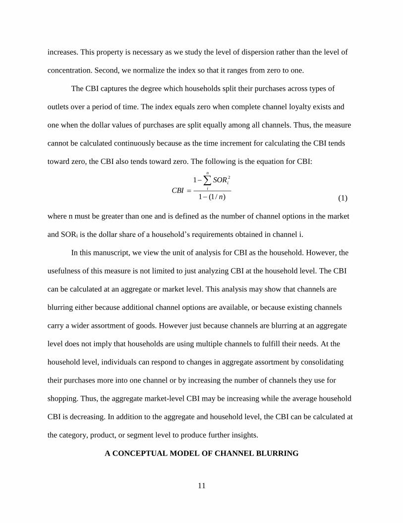
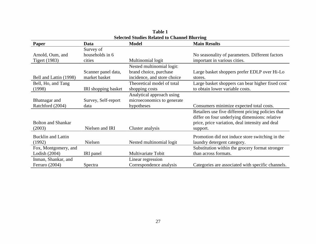2

Channel Blurring


ABSTRACT

Channel blurringmdasha phenomenon in which consumers are moving their purchases of a product

category from channels or retail formats traditionally associated with that category (eg grocery)

to alternative channels (eg mass club extreme valuedollar) and in which retailers from one

channel are selling items traditionally associated with other channelsmdashis of great interest to both

manufacturers and retailers At one time different retail formats such as grocery drug and mass

merchandiser served different purposes but they are becoming indistinguishable For example

large mass merchandisers such as Walmart are now carrying sizeable assortments of grocery

pharmaceutical and electronic products while large drug chains such as Walgreens and CVS are

stocking their shelves with toys and household items We seek to understand how consumers are

responding to these changes We develop a new measure that we call the Channel Blurring

Index which characterizes the degree of channel blurring for a household We develop a model

with the index as a function of demographic behavioral and market factors both at the overall

and at the department levels We estimate the models using data from Nielsenrsquos Homescan

consumer panel for the entire breadth of product categories over a four-year period (2004-2008)

in three cities The results from our analysis offer important substantive insights They show that

households that extensively use private label products (pay lower prices and purchase smaller

baskets of goods) engage in lower (higher) levels of channel blurring Additionally we find that

several demographic factors are associated with the level of channel blurring Importantly the

results suggest that the drivers of channel blurring vary across departments in a retail store

3





















households



4

















format shopping










5























6
























7
























8

























9
























10








the household level















11








(1)















)1(1

12

n

SOR

CBI

n

i

i

12







Demographic Factors

















13


















Behavioral Factors








14










lagged variable














15


blurring index









Market Factors













16




EMPIRICAL STUDY





Data














17













120587(119910 119901 119902) =120548(119901+119902)





120583 =119901

(119901+119902) and 120593 = 119901 + 119902 (3)




Descriptive Results



18












Model Results











19




CBI levels (= -001 p = 010)




















20
























21
























22




DISCUSSION




















23
























24

















25

REFERENCES











17(1) 66-88










4-13











26










68(2) 51-71






















25(5) 457ndash476

27

Table 1



Arnold Oum and

Tigert (1983)

Survey of

households in 6





Scanner panel data

market basket





stores

Bell Ho and Tang



shopping costs



Bhatnagar and

Ratchford (2004)

Survey Self-report

data




Bolton and Shankar





support

Bucklin and Lattin




Fox Montgomery and



than across formats

Inman Shankar and


Linear regression


28

Table 1 Continued


Kumar and Karande

(2000)

AC Nielsen Market




significant

Kumar and Leone







consumer segments

Louviere and Gaeth




Messinger and

Narasimhan (1997)

Aggregate US





convenience

Popkowski-Leszczyc

and Timmermans

(1997) Nielsen



Singh Karsten and

Blattberg (2006)




basket size



29

Table 2


Variable Mean 1 2 3 4 5 6 7 8 9 10 11 12 13 14 15

1 CBIt 0456 1

2 CBIt-1 0456 0629 1

3 Retired HH 0714 -0015 -0017 1

4 Two Wage Earners 0085 -0023 -0018 -0481 1



7 Trip Chaining 5521 0219 0290 0033 -0024 0051 -0106 1

8 Basket Size 46739 -0128 -0163 -0050 0065 -0006 0113 -0046 1


10 Price Index 1045 0002 0014 0003 0001 -0001 0018 -0017 0023 -0035 1



13 Retail Density 3050 -0069 -0070 0002 -0032 -0035 0029 -0097 -0027 -0023 0009 -0143 -0017 1

14 Pittsburgh 0279 0064 0065 -0070 0039 -0106 -0054 0017 -0008 -0071 0004 0001 0011 0011 1

15 Columbus 0465 -0020 -0026 -0057 0038 -0066 0053 -0038 0041 -0007 0001 0030 0025 -0026 -0072 1

30

Table 3




CBIt-1 2687 0008 lt0001

Retired HH -0030 0004 lt0001







Price Index -0002 0001 0001





Columbus 0006 0007 0430

N = 28607

31

Table 4


Dry Groceries

1 Bread


3 Soft Drinks

4 Canned Soup

5 Cookies

Frozen Foods

1 Ice Cream

2 Frozen Pizza

3 Frozen Novelties

4 Frozen Potatoes

5 Frozen Dinners


1 Toothpaste


3 Shampoo

4 Deodorants


32

Table 5A




CBIt-1 2424 0010 lt0001

Retired HH -0037 0005 lt0001












Columbus -0024 0009 0007

Table 5B




CBIt-1 1177 0013 lt0001

Retired HH -0023 0007 lt0001













33

Table 5C




CBIt-1 1031 0010 lt0001






Basket Size 0000 0000 0854








34

Demographic Factors

Retired HH -

Two Wage Earners -

Household Income -


Behavioral Factors

Lag CBI +

Trip Chaining +

Basket Size -


Price Index -


Assortment Depth +

Market Factors

Retail Density +




Figure 1

35

Figure 2


0

100

200

300

400

500

600

700

800

900

Nu

mb

er o

f H

ou

seh

old

s


36

Figure 3


058

059

06

061

062

063

064

065

066C

han

nel

Blu

rrin

g I

nd

ex

37

Figure 4

CBI by Department

0

01

02

03

04

05

06

07

08

09

1


Beauty

Overall

Ch

an

nel

Blu

rrin

g I

nd

ex

38

Appendix A



Table A1




CBIt-1 4571 0003 lt0001






Basket Size -0000 0000 0023








39

Table A2




CBIt-1 2686 0008 lt0001

Retired HH -0030 0004 lt0001












Columbus 0006 0007 0396

40

Table A3




CBIt-1 2687 0008 lt0001

Retired HH -0030 0004 lt0001







Price Index -0002 0001 0001





Columbus 0006 0007 0430

2nd Quarter 2005 -0001 0010 0901

3rd Quarter 2005 0058 0010 lt0001

4th Quarter 2005 0101 0010 lt0001

1st Quarter 2006 -0040 0010 lt0001

2nd Quarter 2006 -0002 0010 0862

3rd Quarter 2006 0035 0010 lt0001

4th Quarter 2006 0096 0010 lt0001

1st Quarter 2007 -0007 0010 0489

2nd Quarter 2007 0045 0010 lt0001

3rd Quarter 2007 0036 0010 lt0001

4th Quarter 2007 0069 0010 lt0001

1st Quarter 2008 -0022 0011 0040

2nd Quarter 2008 -0001 0010 0902

3rd Quarter 2008 0025 0010 0017

Scale( 6329 0050




3





















households



4

















format shopping










5























6
























7
























8

























9
























10








the household level















11








(1)















)1(1

12

n

SOR

CBI

n

i

i

12







Demographic Factors

















13


















Behavioral Factors








14










lagged variable














15


blurring index









Market Factors













16




EMPIRICAL STUDY





Data














17













120587(119910 119901 119902) =120548(119901+119902)





120583 =119901

(119901+119902) and 120593 = 119901 + 119902 (3)




Descriptive Results



18












Model Results











19




CBI levels (= -001 p = 010)




















20
























21
























22




DISCUSSION




















23
























24

















25

REFERENCES











17(1) 66-88










4-13











26










68(2) 51-71






















25(5) 457ndash476

27

Table 1



Arnold Oum and

Tigert (1983)

Survey of

households in 6





Scanner panel data

market basket





stores

Bell Ho and Tang



shopping costs



Bhatnagar and

Ratchford (2004)

Survey Self-report

data




Bolton and Shankar





support

Bucklin and Lattin




Fox Montgomery and



than across formats

Inman Shankar and


Linear regression


28

Table 1 Continued


Kumar and Karande

(2000)

AC Nielsen Market




significant

Kumar and Leone







consumer segments

Louviere and Gaeth




Messinger and

Narasimhan (1997)

Aggregate US





convenience

Popkowski-Leszczyc

and Timmermans

(1997) Nielsen



Singh Karsten and

Blattberg (2006)




basket size



29

Table 2


Variable Mean 1 2 3 4 5 6 7 8 9 10 11 12 13 14 15

1 CBIt 0456 1

2 CBIt-1 0456 0629 1

3 Retired HH 0714 -0015 -0017 1

4 Two Wage Earners 0085 -0023 -0018 -0481 1



7 Trip Chaining 5521 0219 0290 0033 -0024 0051 -0106 1

8 Basket Size 46739 -0128 -0163 -0050 0065 -0006 0113 -0046 1


10 Price Index 1045 0002 0014 0003 0001 -0001 0018 -0017 0023 -0035 1



13 Retail Density 3050 -0069 -0070 0002 -0032 -0035 0029 -0097 -0027 -0023 0009 -0143 -0017 1

14 Pittsburgh 0279 0064 0065 -0070 0039 -0106 -0054 0017 -0008 -0071 0004 0001 0011 0011 1

15 Columbus 0465 -0020 -0026 -0057 0038 -0066 0053 -0038 0041 -0007 0001 0030 0025 -0026 -0072 1

30

Table 3




CBIt-1 2687 0008 lt0001

Retired HH -0030 0004 lt0001







Price Index -0002 0001 0001





Columbus 0006 0007 0430

N = 28607

31

Table 4


Dry Groceries

1 Bread


3 Soft Drinks

4 Canned Soup

5 Cookies

Frozen Foods

1 Ice Cream

2 Frozen Pizza

3 Frozen Novelties

4 Frozen Potatoes

5 Frozen Dinners


1 Toothpaste


3 Shampoo

4 Deodorants


32

Table 5A




CBIt-1 2424 0010 lt0001

Retired HH -0037 0005 lt0001












Columbus -0024 0009 0007

Table 5B




CBIt-1 1177 0013 lt0001

Retired HH -0023 0007 lt0001













33

Table 5C




CBIt-1 1031 0010 lt0001






Basket Size 0000 0000 0854








34

Demographic Factors

Retired HH -

Two Wage Earners -

Household Income -


Behavioral Factors

Lag CBI +

Trip Chaining +

Basket Size -


Price Index -


Assortment Depth +

Market Factors

Retail Density +




Figure 1

35

Figure 2


0

100

200

300

400

500

600

700

800

900

Nu

mb

er o

f H

ou

seh

old

s


36

Figure 3


058

059

06

061

062

063

064

065

066C

han

nel

Blu

rrin

g I

nd

ex

37

Figure 4

CBI by Department

0

01

02

03

04

05

06

07

08

09

1


Beauty

Overall

Ch

an

nel

Blu

rrin

g I

nd

ex

38

Appendix A



Table A1




CBIt-1 4571 0003 lt0001






Basket Size -0000 0000 0023








39

Table A2




CBIt-1 2686 0008 lt0001

Retired HH -0030 0004 lt0001












Columbus 0006 0007 0396

40

Table A3




CBIt-1 2687 0008 lt0001

Retired HH -0030 0004 lt0001







Price Index -0002 0001 0001





Columbus 0006 0007 0430

2nd Quarter 2005 -0001 0010 0901

3rd Quarter 2005 0058 0010 lt0001

4th Quarter 2005 0101 0010 lt0001

1st Quarter 2006 -0040 0010 lt0001

2nd Quarter 2006 -0002 0010 0862

3rd Quarter 2006 0035 0010 lt0001

4th Quarter 2006 0096 0010 lt0001

1st Quarter 2007 -0007 0010 0489

2nd Quarter 2007 0045 0010 lt0001

3rd Quarter 2007 0036 0010 lt0001

4th Quarter 2007 0069 0010 lt0001

1st Quarter 2008 -0022 0011 0040

2nd Quarter 2008 -0001 0010 0902

3rd Quarter 2008 0025 0010 0017

Scale( 6329 0050




4

















format shopping










5























6
























7
























8

























9
























10








the household level















11








(1)















)1(1

12

n

SOR

CBI

n

i

i

12







Demographic Factors

















13


















Behavioral Factors








14










lagged variable














15


blurring index









Market Factors













16




EMPIRICAL STUDY





Data














17













120587(119910 119901 119902) =120548(119901+119902)





120583 =119901

(119901+119902) and 120593 = 119901 + 119902 (3)




Descriptive Results



18












Model Results











19




CBI levels (= -001 p = 010)




















20
























21
























22




DISCUSSION




















23
























24

















25

REFERENCES











17(1) 66-88










4-13











26










68(2) 51-71






















25(5) 457ndash476

27

Table 1



Arnold Oum and

Tigert (1983)

Survey of

households in 6





Scanner panel data

market basket





stores

Bell Ho and Tang



shopping costs



Bhatnagar and

Ratchford (2004)

Survey Self-report

data




Bolton and Shankar





support

Bucklin and Lattin




Fox Montgomery and



than across formats

Inman Shankar and


Linear regression


28

Table 1 Continued


Kumar and Karande

(2000)

AC Nielsen Market




significant

Kumar and Leone







consumer segments

Louviere and Gaeth




Messinger and

Narasimhan (1997)

Aggregate US





convenience

Popkowski-Leszczyc

and Timmermans

(1997) Nielsen



Singh Karsten and

Blattberg (2006)




basket size



29

Table 2


Variable Mean 1 2 3 4 5 6 7 8 9 10 11 12 13 14 15

1 CBIt 0456 1

2 CBIt-1 0456 0629 1

3 Retired HH 0714 -0015 -0017 1

4 Two Wage Earners 0085 -0023 -0018 -0481 1



7 Trip Chaining 5521 0219 0290 0033 -0024 0051 -0106 1

8 Basket Size 46739 -0128 -0163 -0050 0065 -0006 0113 -0046 1


10 Price Index 1045 0002 0014 0003 0001 -0001 0018 -0017 0023 -0035 1



13 Retail Density 3050 -0069 -0070 0002 -0032 -0035 0029 -0097 -0027 -0023 0009 -0143 -0017 1

14 Pittsburgh 0279 0064 0065 -0070 0039 -0106 -0054 0017 -0008 -0071 0004 0001 0011 0011 1

15 Columbus 0465 -0020 -0026 -0057 0038 -0066 0053 -0038 0041 -0007 0001 0030 0025 -0026 -0072 1

30

Table 3




CBIt-1 2687 0008 lt0001

Retired HH -0030 0004 lt0001







Price Index -0002 0001 0001





Columbus 0006 0007 0430

N = 28607

31

Table 4


Dry Groceries

1 Bread


3 Soft Drinks

4 Canned Soup

5 Cookies

Frozen Foods

1 Ice Cream

2 Frozen Pizza

3 Frozen Novelties

4 Frozen Potatoes

5 Frozen Dinners


1 Toothpaste


3 Shampoo

4 Deodorants


32

Table 5A




CBIt-1 2424 0010 lt0001

Retired HH -0037 0005 lt0001












Columbus -0024 0009 0007

Table 5B




CBIt-1 1177 0013 lt0001

Retired HH -0023 0007 lt0001













33

Table 5C




CBIt-1 1031 0010 lt0001






Basket Size 0000 0000 0854








34

Demographic Factors

Retired HH -

Two Wage Earners -

Household Income -


Behavioral Factors

Lag CBI +

Trip Chaining +

Basket Size -


Price Index -


Assortment Depth +

Market Factors

Retail Density +




Figure 1

35

Figure 2


0

100

200

300

400

500

600

700

800

900

Nu

mb

er o

f H

ou

seh

old

s


36

Figure 3


058

059

06

061

062

063

064

065

066C

han

nel

Blu

rrin

g I

nd

ex

37

Figure 4

CBI by Department

0

01

02

03

04

05

06

07

08

09

1


Beauty

Overall

Ch

an

nel

Blu

rrin

g I

nd

ex

38

Appendix A



Table A1




CBIt-1 4571 0003 lt0001






Basket Size -0000 0000 0023








39

Table A2




CBIt-1 2686 0008 lt0001

Retired HH -0030 0004 lt0001












Columbus 0006 0007 0396

40

Table A3




CBIt-1 2687 0008 lt0001

Retired HH -0030 0004 lt0001







Price Index -0002 0001 0001





Columbus 0006 0007 0430

2nd Quarter 2005 -0001 0010 0901

3rd Quarter 2005 0058 0010 lt0001

4th Quarter 2005 0101 0010 lt0001

1st Quarter 2006 -0040 0010 lt0001

2nd Quarter 2006 -0002 0010 0862

3rd Quarter 2006 0035 0010 lt0001

4th Quarter 2006 0096 0010 lt0001

1st Quarter 2007 -0007 0010 0489

2nd Quarter 2007 0045 0010 lt0001

3rd Quarter 2007 0036 0010 lt0001

4th Quarter 2007 0069 0010 lt0001

1st Quarter 2008 -0022 0011 0040

2nd Quarter 2008 -0001 0010 0902

3rd Quarter 2008 0025 0010 0017

Scale( 6329 0050




5























6
























7
























8

























9
























10








the household level















11








(1)















)1(1

12

n

SOR

CBI

n

i

i

12







Demographic Factors

















13


















Behavioral Factors








14










lagged variable














15


blurring index









Market Factors













16




EMPIRICAL STUDY





Data














17













120587(119910 119901 119902) =120548(119901+119902)





120583 =119901

(119901+119902) and 120593 = 119901 + 119902 (3)




Descriptive Results



18












Model Results











19




CBI levels (= -001 p = 010)




















20
























21
























22




DISCUSSION




















23
























24

















25

REFERENCES











17(1) 66-88










4-13











26










68(2) 51-71






















25(5) 457ndash476

27

Table 1



Arnold Oum and

Tigert (1983)

Survey of

households in 6





Scanner panel data

market basket





stores

Bell Ho and Tang



shopping costs



Bhatnagar and

Ratchford (2004)

Survey Self-report

data




Bolton and Shankar





support

Bucklin and Lattin




Fox Montgomery and



than across formats

Inman Shankar and


Linear regression


28

Table 1 Continued


Kumar and Karande

(2000)

AC Nielsen Market




significant

Kumar and Leone







consumer segments

Louviere and Gaeth




Messinger and

Narasimhan (1997)

Aggregate US





convenience

Popkowski-Leszczyc

and Timmermans

(1997) Nielsen



Singh Karsten and

Blattberg (2006)




basket size



29

Table 2


Variable Mean 1 2 3 4 5 6 7 8 9 10 11 12 13 14 15

1 CBIt 0456 1

2 CBIt-1 0456 0629 1

3 Retired HH 0714 -0015 -0017 1

4 Two Wage Earners 0085 -0023 -0018 -0481 1



7 Trip Chaining 5521 0219 0290 0033 -0024 0051 -0106 1

8 Basket Size 46739 -0128 -0163 -0050 0065 -0006 0113 -0046 1


10 Price Index 1045 0002 0014 0003 0001 -0001 0018 -0017 0023 -0035 1



13 Retail Density 3050 -0069 -0070 0002 -0032 -0035 0029 -0097 -0027 -0023 0009 -0143 -0017 1

14 Pittsburgh 0279 0064 0065 -0070 0039 -0106 -0054 0017 -0008 -0071 0004 0001 0011 0011 1

15 Columbus 0465 -0020 -0026 -0057 0038 -0066 0053 -0038 0041 -0007 0001 0030 0025 -0026 -0072 1

30

Table 3




CBIt-1 2687 0008 lt0001

Retired HH -0030 0004 lt0001







Price Index -0002 0001 0001





Columbus 0006 0007 0430

N = 28607

31

Table 4


Dry Groceries

1 Bread


3 Soft Drinks

4 Canned Soup

5 Cookies

Frozen Foods

1 Ice Cream

2 Frozen Pizza

3 Frozen Novelties

4 Frozen Potatoes

5 Frozen Dinners


1 Toothpaste


3 Shampoo

4 Deodorants


32

Table 5A




CBIt-1 2424 0010 lt0001

Retired HH -0037 0005 lt0001












Columbus -0024 0009 0007

Table 5B




CBIt-1 1177 0013 lt0001

Retired HH -0023 0007 lt0001













33

Table 5C




CBIt-1 1031 0010 lt0001






Basket Size 0000 0000 0854








34

Demographic Factors

Retired HH -

Two Wage Earners -

Household Income -


Behavioral Factors

Lag CBI +

Trip Chaining +

Basket Size -


Price Index -


Assortment Depth +

Market Factors

Retail Density +




Figure 1

35

Figure 2


0

100

200

300

400

500

600

700

800

900

Nu

mb

er o

f H

ou

seh

old

s


36

Figure 3


058

059

06

061

062

063

064

065

066C

han

nel

Blu

rrin

g I

nd

ex

37

Figure 4

CBI by Department

0

01

02

03

04

05

06

07

08

09

1


Beauty

Overall

Ch

an

nel

Blu

rrin

g I

nd

ex

38

Appendix A



Table A1




CBIt-1 4571 0003 lt0001






Basket Size -0000 0000 0023








39

Table A2




CBIt-1 2686 0008 lt0001

Retired HH -0030 0004 lt0001












Columbus 0006 0007 0396

40

Table A3




CBIt-1 2687 0008 lt0001

Retired HH -0030 0004 lt0001







Price Index -0002 0001 0001





Columbus 0006 0007 0430

2nd Quarter 2005 -0001 0010 0901

3rd Quarter 2005 0058 0010 lt0001

4th Quarter 2005 0101 0010 lt0001

1st Quarter 2006 -0040 0010 lt0001

2nd Quarter 2006 -0002 0010 0862

3rd Quarter 2006 0035 0010 lt0001

4th Quarter 2006 0096 0010 lt0001

1st Quarter 2007 -0007 0010 0489

2nd Quarter 2007 0045 0010 lt0001

3rd Quarter 2007 0036 0010 lt0001

4th Quarter 2007 0069 0010 lt0001

1st Quarter 2008 -0022 0011 0040

2nd Quarter 2008 -0001 0010 0902

3rd Quarter 2008 0025 0010 0017

Scale( 6329 0050




6
























7
























8

























9
























10








the household level















11








(1)















)1(1

12

n

SOR

CBI

n

i

i

12







Demographic Factors

















13


















Behavioral Factors








14










lagged variable














15


blurring index









Market Factors













16




EMPIRICAL STUDY





Data














17













120587(119910 119901 119902) =120548(119901+119902)





120583 =119901

(119901+119902) and 120593 = 119901 + 119902 (3)




Descriptive Results



18












Model Results











19




CBI levels (= -001 p = 010)




















20
























21
























22




DISCUSSION




















23
























24

















25

REFERENCES











17(1) 66-88










4-13











26










68(2) 51-71






















25(5) 457ndash476

27

Table 1



Arnold Oum and

Tigert (1983)

Survey of

households in 6





Scanner panel data

market basket





stores

Bell Ho and Tang



shopping costs



Bhatnagar and

Ratchford (2004)

Survey Self-report

data




Bolton and Shankar





support

Bucklin and Lattin




Fox Montgomery and



than across formats

Inman Shankar and


Linear regression


28

Table 1 Continued


Kumar and Karande

(2000)

AC Nielsen Market




significant

Kumar and Leone







consumer segments

Louviere and Gaeth




Messinger and

Narasimhan (1997)

Aggregate US





convenience

Popkowski-Leszczyc

and Timmermans

(1997) Nielsen



Singh Karsten and

Blattberg (2006)




basket size



29

Table 2


Variable Mean 1 2 3 4 5 6 7 8 9 10 11 12 13 14 15

1 CBIt 0456 1

2 CBIt-1 0456 0629 1

3 Retired HH 0714 -0015 -0017 1

4 Two Wage Earners 0085 -0023 -0018 -0481 1



7 Trip Chaining 5521 0219 0290 0033 -0024 0051 -0106 1

8 Basket Size 46739 -0128 -0163 -0050 0065 -0006 0113 -0046 1


10 Price Index 1045 0002 0014 0003 0001 -0001 0018 -0017 0023 -0035 1



13 Retail Density 3050 -0069 -0070 0002 -0032 -0035 0029 -0097 -0027 -0023 0009 -0143 -0017 1

14 Pittsburgh 0279 0064 0065 -0070 0039 -0106 -0054 0017 -0008 -0071 0004 0001 0011 0011 1

15 Columbus 0465 -0020 -0026 -0057 0038 -0066 0053 -0038 0041 -0007 0001 0030 0025 -0026 -0072 1

30

Table 3




CBIt-1 2687 0008 lt0001

Retired HH -0030 0004 lt0001







Price Index -0002 0001 0001





Columbus 0006 0007 0430

N = 28607

31

Table 4


Dry Groceries

1 Bread


3 Soft Drinks

4 Canned Soup

5 Cookies

Frozen Foods

1 Ice Cream

2 Frozen Pizza

3 Frozen Novelties

4 Frozen Potatoes

5 Frozen Dinners


1 Toothpaste


3 Shampoo

4 Deodorants


32

Table 5A




CBIt-1 2424 0010 lt0001

Retired HH -0037 0005 lt0001












Columbus -0024 0009 0007

Table 5B




CBIt-1 1177 0013 lt0001

Retired HH -0023 0007 lt0001













33

Table 5C




CBIt-1 1031 0010 lt0001






Basket Size 0000 0000 0854








34

Demographic Factors

Retired HH -

Two Wage Earners -

Household Income -


Behavioral Factors

Lag CBI +

Trip Chaining +

Basket Size -


Price Index -


Assortment Depth +

Market Factors

Retail Density +




Figure 1

35

Figure 2


0

100

200

300

400

500

600

700

800

900

Nu

mb

er o

f H

ou

seh

old

s


36

Figure 3


058

059

06

061

062

063

064

065

066C

han

nel

Blu

rrin

g I

nd

ex

37

Figure 4

CBI by Department

0

01

02

03

04

05

06

07

08

09

1


Beauty

Overall

Ch

an

nel

Blu

rrin

g I

nd

ex

38

Appendix A



Table A1




CBIt-1 4571 0003 lt0001






Basket Size -0000 0000 0023








39

Table A2




CBIt-1 2686 0008 lt0001

Retired HH -0030 0004 lt0001












Columbus 0006 0007 0396

40

Table A3




CBIt-1 2687 0008 lt0001

Retired HH -0030 0004 lt0001







Price Index -0002 0001 0001





Columbus 0006 0007 0430

2nd Quarter 2005 -0001 0010 0901

3rd Quarter 2005 0058 0010 lt0001

4th Quarter 2005 0101 0010 lt0001

1st Quarter 2006 -0040 0010 lt0001

2nd Quarter 2006 -0002 0010 0862

3rd Quarter 2006 0035 0010 lt0001

4th Quarter 2006 0096 0010 lt0001

1st Quarter 2007 -0007 0010 0489

2nd Quarter 2007 0045 0010 lt0001

3rd Quarter 2007 0036 0010 lt0001

4th Quarter 2007 0069 0010 lt0001

1st Quarter 2008 -0022 0011 0040

2nd Quarter 2008 -0001 0010 0902

3rd Quarter 2008 0025 0010 0017

Scale( 6329 0050




7
























8

























9
























10








the household level















11








(1)















)1(1

12

n

SOR

CBI

n

i

i

12







Demographic Factors

















13


















Behavioral Factors








14










lagged variable














15


blurring index









Market Factors













16




EMPIRICAL STUDY





Data














17













120587(119910 119901 119902) =120548(119901+119902)





120583 =119901

(119901+119902) and 120593 = 119901 + 119902 (3)




Descriptive Results



18












Model Results











19




CBI levels (= -001 p = 010)




















20
























21
























22




DISCUSSION




















23
























24

















25

REFERENCES











17(1) 66-88










4-13











26










68(2) 51-71






















25(5) 457ndash476

27

Table 1



Arnold Oum and

Tigert (1983)

Survey of

households in 6





Scanner panel data

market basket





stores

Bell Ho and Tang



shopping costs



Bhatnagar and

Ratchford (2004)

Survey Self-report

data




Bolton and Shankar





support

Bucklin and Lattin




Fox Montgomery and



than across formats

Inman Shankar and


Linear regression


28

Table 1 Continued


Kumar and Karande

(2000)

AC Nielsen Market




significant

Kumar and Leone







consumer segments

Louviere and Gaeth




Messinger and

Narasimhan (1997)

Aggregate US





convenience

Popkowski-Leszczyc

and Timmermans

(1997) Nielsen



Singh Karsten and

Blattberg (2006)




basket size



29

Table 2


Variable Mean 1 2 3 4 5 6 7 8 9 10 11 12 13 14 15

1 CBIt 0456 1

2 CBIt-1 0456 0629 1

3 Retired HH 0714 -0015 -0017 1

4 Two Wage Earners 0085 -0023 -0018 -0481 1



7 Trip Chaining 5521 0219 0290 0033 -0024 0051 -0106 1

8 Basket Size 46739 -0128 -0163 -0050 0065 -0006 0113 -0046 1


10 Price Index 1045 0002 0014 0003 0001 -0001 0018 -0017 0023 -0035 1



13 Retail Density 3050 -0069 -0070 0002 -0032 -0035 0029 -0097 -0027 -0023 0009 -0143 -0017 1

14 Pittsburgh 0279 0064 0065 -0070 0039 -0106 -0054 0017 -0008 -0071 0004 0001 0011 0011 1

15 Columbus 0465 -0020 -0026 -0057 0038 -0066 0053 -0038 0041 -0007 0001 0030 0025 -0026 -0072 1

30

Table 3




CBIt-1 2687 0008 lt0001

Retired HH -0030 0004 lt0001







Price Index -0002 0001 0001





Columbus 0006 0007 0430

N = 28607

31

Table 4


Dry Groceries

1 Bread


3 Soft Drinks

4 Canned Soup

5 Cookies

Frozen Foods

1 Ice Cream

2 Frozen Pizza

3 Frozen Novelties

4 Frozen Potatoes

5 Frozen Dinners


1 Toothpaste


3 Shampoo

4 Deodorants


32

Table 5A




CBIt-1 2424 0010 lt0001

Retired HH -0037 0005 lt0001












Columbus -0024 0009 0007

Table 5B




CBIt-1 1177 0013 lt0001

Retired HH -0023 0007 lt0001













33

Table 5C




CBIt-1 1031 0010 lt0001






Basket Size 0000 0000 0854








34

Demographic Factors

Retired HH -

Two Wage Earners -

Household Income -


Behavioral Factors

Lag CBI +

Trip Chaining +

Basket Size -


Price Index -


Assortment Depth +

Market Factors

Retail Density +




Figure 1

35

Figure 2


0

100

200

300

400

500

600

700

800

900

Nu

mb

er o

f H

ou

seh

old

s


36

Figure 3


058

059

06

061

062

063

064

065

066C

han

nel

Blu

rrin

g I

nd

ex

37

Figure 4

CBI by Department

0

01

02

03

04

05

06

07

08

09

1


Beauty

Overall

Ch

an

nel

Blu

rrin

g I

nd

ex

38

Appendix A



Table A1




CBIt-1 4571 0003 lt0001






Basket Size -0000 0000 0023








39

Table A2




CBIt-1 2686 0008 lt0001

Retired HH -0030 0004 lt0001












Columbus 0006 0007 0396

40

Table A3




CBIt-1 2687 0008 lt0001

Retired HH -0030 0004 lt0001







Price Index -0002 0001 0001





Columbus 0006 0007 0430

2nd Quarter 2005 -0001 0010 0901

3rd Quarter 2005 0058 0010 lt0001

4th Quarter 2005 0101 0010 lt0001

1st Quarter 2006 -0040 0010 lt0001

2nd Quarter 2006 -0002 0010 0862

3rd Quarter 2006 0035 0010 lt0001

4th Quarter 2006 0096 0010 lt0001

1st Quarter 2007 -0007 0010 0489

2nd Quarter 2007 0045 0010 lt0001

3rd Quarter 2007 0036 0010 lt0001

4th Quarter 2007 0069 0010 lt0001

1st Quarter 2008 -0022 0011 0040

2nd Quarter 2008 -0001 0010 0902

3rd Quarter 2008 0025 0010 0017

Scale( 6329 0050




8

























9
























10








the household level















11








(1)















)1(1

12

n

SOR

CBI

n

i

i

12







Demographic Factors

















13


















Behavioral Factors








14










lagged variable














15


blurring index









Market Factors













16




EMPIRICAL STUDY





Data














17













120587(119910 119901 119902) =120548(119901+119902)





120583 =119901

(119901+119902) and 120593 = 119901 + 119902 (3)




Descriptive Results



18












Model Results











19




CBI levels (= -001 p = 010)




















20
























21
























22




DISCUSSION




















23
























24

















25

REFERENCES











17(1) 66-88










4-13











26










68(2) 51-71






















25(5) 457ndash476

27

Table 1



Arnold Oum and

Tigert (1983)

Survey of

households in 6





Scanner panel data

market basket





stores

Bell Ho and Tang



shopping costs



Bhatnagar and

Ratchford (2004)

Survey Self-report

data




Bolton and Shankar





support

Bucklin and Lattin




Fox Montgomery and



than across formats

Inman Shankar and


Linear regression


28

Table 1 Continued


Kumar and Karande

(2000)

AC Nielsen Market




significant

Kumar and Leone







consumer segments

Louviere and Gaeth




Messinger and

Narasimhan (1997)

Aggregate US





convenience

Popkowski-Leszczyc

and Timmermans

(1997) Nielsen



Singh Karsten and

Blattberg (2006)




basket size



29

Table 2


Variable Mean 1 2 3 4 5 6 7 8 9 10 11 12 13 14 15

1 CBIt 0456 1

2 CBIt-1 0456 0629 1

3 Retired HH 0714 -0015 -0017 1

4 Two Wage Earners 0085 -0023 -0018 -0481 1



7 Trip Chaining 5521 0219 0290 0033 -0024 0051 -0106 1

8 Basket Size 46739 -0128 -0163 -0050 0065 -0006 0113 -0046 1


10 Price Index 1045 0002 0014 0003 0001 -0001 0018 -0017 0023 -0035 1



13 Retail Density 3050 -0069 -0070 0002 -0032 -0035 0029 -0097 -0027 -0023 0009 -0143 -0017 1

14 Pittsburgh 0279 0064 0065 -0070 0039 -0106 -0054 0017 -0008 -0071 0004 0001 0011 0011 1

15 Columbus 0465 -0020 -0026 -0057 0038 -0066 0053 -0038 0041 -0007 0001 0030 0025 -0026 -0072 1

30

Table 3




CBIt-1 2687 0008 lt0001

Retired HH -0030 0004 lt0001







Price Index -0002 0001 0001





Columbus 0006 0007 0430

N = 28607

31

Table 4


Dry Groceries

1 Bread


3 Soft Drinks

4 Canned Soup

5 Cookies

Frozen Foods

1 Ice Cream

2 Frozen Pizza

3 Frozen Novelties

4 Frozen Potatoes

5 Frozen Dinners


1 Toothpaste


3 Shampoo

4 Deodorants


32

Table 5A




CBIt-1 2424 0010 lt0001

Retired HH -0037 0005 lt0001












Columbus -0024 0009 0007

Table 5B




CBIt-1 1177 0013 lt0001

Retired HH -0023 0007 lt0001













33

Table 5C




CBIt-1 1031 0010 lt0001






Basket Size 0000 0000 0854








34

Demographic Factors

Retired HH -

Two Wage Earners -

Household Income -


Behavioral Factors

Lag CBI +

Trip Chaining +

Basket Size -


Price Index -


Assortment Depth +

Market Factors

Retail Density +




Figure 1

35

Figure 2


0

100

200

300

400

500

600

700

800

900

Nu

mb

er o

f H

ou

seh

old

s


36

Figure 3


058

059

06

061

062

063

064

065

066C

han

nel

Blu

rrin

g I

nd

ex

37

Figure 4

CBI by Department

0

01

02

03

04

05

06

07

08

09

1


Beauty

Overall

Ch

an

nel

Blu

rrin

g I

nd

ex

38

Appendix A



Table A1




CBIt-1 4571 0003 lt0001






Basket Size -0000 0000 0023








39

Table A2




CBIt-1 2686 0008 lt0001

Retired HH -0030 0004 lt0001












Columbus 0006 0007 0396

40

Table A3




CBIt-1 2687 0008 lt0001

Retired HH -0030 0004 lt0001







Price Index -0002 0001 0001





Columbus 0006 0007 0430

2nd Quarter 2005 -0001 0010 0901

3rd Quarter 2005 0058 0010 lt0001

4th Quarter 2005 0101 0010 lt0001

1st Quarter 2006 -0040 0010 lt0001

2nd Quarter 2006 -0002 0010 0862

3rd Quarter 2006 0035 0010 lt0001

4th Quarter 2006 0096 0010 lt0001

1st Quarter 2007 -0007 0010 0489

2nd Quarter 2007 0045 0010 lt0001

3rd Quarter 2007 0036 0010 lt0001

4th Quarter 2007 0069 0010 lt0001

1st Quarter 2008 -0022 0011 0040

2nd Quarter 2008 -0001 0010 0902

3rd Quarter 2008 0025 0010 0017

Scale( 6329 0050




9
























10








the household level















11








(1)















)1(1

12

n

SOR

CBI

n

i

i

12







Demographic Factors

















13


















Behavioral Factors








14










lagged variable














15


blurring index









Market Factors













16




EMPIRICAL STUDY





Data














17













120587(119910 119901 119902) =120548(119901+119902)





120583 =119901

(119901+119902) and 120593 = 119901 + 119902 (3)




Descriptive Results



18












Model Results











19




CBI levels (= -001 p = 010)




















20
























21
























22




DISCUSSION




















23
























24

















25

REFERENCES











17(1) 66-88










4-13











26










68(2) 51-71






















25(5) 457ndash476

27

Table 1



Arnold Oum and

Tigert (1983)

Survey of

households in 6





Scanner panel data

market basket





stores

Bell Ho and Tang



shopping costs



Bhatnagar and

Ratchford (2004)

Survey Self-report

data




Bolton and Shankar





support

Bucklin and Lattin




Fox Montgomery and



than across formats

Inman Shankar and


Linear regression


28

Table 1 Continued


Kumar and Karande

(2000)

AC Nielsen Market




significant

Kumar and Leone







consumer segments

Louviere and Gaeth




Messinger and

Narasimhan (1997)

Aggregate US





convenience

Popkowski-Leszczyc

and Timmermans

(1997) Nielsen



Singh Karsten and

Blattberg (2006)




basket size



29

Table 2


Variable Mean 1 2 3 4 5 6 7 8 9 10 11 12 13 14 15

1 CBIt 0456 1

2 CBIt-1 0456 0629 1

3 Retired HH 0714 -0015 -0017 1

4 Two Wage Earners 0085 -0023 -0018 -0481 1



7 Trip Chaining 5521 0219 0290 0033 -0024 0051 -0106 1

8 Basket Size 46739 -0128 -0163 -0050 0065 -0006 0113 -0046 1


10 Price Index 1045 0002 0014 0003 0001 -0001 0018 -0017 0023 -0035 1



13 Retail Density 3050 -0069 -0070 0002 -0032 -0035 0029 -0097 -0027 -0023 0009 -0143 -0017 1

14 Pittsburgh 0279 0064 0065 -0070 0039 -0106 -0054 0017 -0008 -0071 0004 0001 0011 0011 1

15 Columbus 0465 -0020 -0026 -0057 0038 -0066 0053 -0038 0041 -0007 0001 0030 0025 -0026 -0072 1

30

Table 3




CBIt-1 2687 0008 lt0001

Retired HH -0030 0004 lt0001







Price Index -0002 0001 0001





Columbus 0006 0007 0430

N = 28607

31

Table 4


Dry Groceries

1 Bread


3 Soft Drinks

4 Canned Soup

5 Cookies

Frozen Foods

1 Ice Cream

2 Frozen Pizza

3 Frozen Novelties

4 Frozen Potatoes

5 Frozen Dinners


1 Toothpaste


3 Shampoo

4 Deodorants


32

Table 5A




CBIt-1 2424 0010 lt0001

Retired HH -0037 0005 lt0001












Columbus -0024 0009 0007

Table 5B




CBIt-1 1177 0013 lt0001

Retired HH -0023 0007 lt0001













33

Table 5C




CBIt-1 1031 0010 lt0001






Basket Size 0000 0000 0854








34

Demographic Factors

Retired HH -

Two Wage Earners -

Household Income -


Behavioral Factors

Lag CBI +

Trip Chaining +

Basket Size -


Price Index -


Assortment Depth +

Market Factors

Retail Density +




Figure 1

35

Figure 2


0

100

200

300

400

500

600

700

800

900

Nu

mb

er o

f H

ou

seh

old

s


36

Figure 3


058

059

06

061

062

063

064

065

066C

han

nel

Blu

rrin

g I

nd

ex

37

Figure 4

CBI by Department

0

01

02

03

04

05

06

07

08

09

1


Beauty

Overall

Ch

an

nel

Blu

rrin

g I

nd

ex

38

Appendix A



Table A1




CBIt-1 4571 0003 lt0001






Basket Size -0000 0000 0023








39

Table A2




CBIt-1 2686 0008 lt0001

Retired HH -0030 0004 lt0001












Columbus 0006 0007 0396

40

Table A3




CBIt-1 2687 0008 lt0001

Retired HH -0030 0004 lt0001







Price Index -0002 0001 0001





Columbus 0006 0007 0430

2nd Quarter 2005 -0001 0010 0901

3rd Quarter 2005 0058 0010 lt0001

4th Quarter 2005 0101 0010 lt0001

1st Quarter 2006 -0040 0010 lt0001

2nd Quarter 2006 -0002 0010 0862

3rd Quarter 2006 0035 0010 lt0001

4th Quarter 2006 0096 0010 lt0001

1st Quarter 2007 -0007 0010 0489

2nd Quarter 2007 0045 0010 lt0001

3rd Quarter 2007 0036 0010 lt0001

4th Quarter 2007 0069 0010 lt0001

1st Quarter 2008 -0022 0011 0040

2nd Quarter 2008 -0001 0010 0902

3rd Quarter 2008 0025 0010 0017

Scale( 6329 0050




10








the household level















11








(1)















)1(1

12

n

SOR

CBI

n

i

i

12







Demographic Factors

















13


















Behavioral Factors








14










lagged variable














15


blurring index









Market Factors













16




EMPIRICAL STUDY





Data














17













120587(119910 119901 119902) =120548(119901+119902)





120583 =119901

(119901+119902) and 120593 = 119901 + 119902 (3)




Descriptive Results



18












Model Results











19




CBI levels (= -001 p = 010)




















20
























21
























22




DISCUSSION




















23
























24

















25

REFERENCES











17(1) 66-88










4-13











26










68(2) 51-71






















25(5) 457ndash476

27

Table 1



Arnold Oum and

Tigert (1983)

Survey of

households in 6





Scanner panel data

market basket





stores

Bell Ho and Tang



shopping costs



Bhatnagar and

Ratchford (2004)

Survey Self-report

data




Bolton and Shankar





support

Bucklin and Lattin




Fox Montgomery and



than across formats

Inman Shankar and


Linear regression


28

Table 1 Continued


Kumar and Karande

(2000)

AC Nielsen Market




significant

Kumar and Leone







consumer segments

Louviere and Gaeth




Messinger and

Narasimhan (1997)

Aggregate US





convenience

Popkowski-Leszczyc

and Timmermans

(1997) Nielsen



Singh Karsten and

Blattberg (2006)




basket size



29

Table 2


Variable Mean 1 2 3 4 5 6 7 8 9 10 11 12 13 14 15

1 CBIt 0456 1

2 CBIt-1 0456 0629 1

3 Retired HH 0714 -0015 -0017 1

4 Two Wage Earners 0085 -0023 -0018 -0481 1



7 Trip Chaining 5521 0219 0290 0033 -0024 0051 -0106 1

8 Basket Size 46739 -0128 -0163 -0050 0065 -0006 0113 -0046 1


10 Price Index 1045 0002 0014 0003 0001 -0001 0018 -0017 0023 -0035 1



13 Retail Density 3050 -0069 -0070 0002 -0032 -0035 0029 -0097 -0027 -0023 0009 -0143 -0017 1

14 Pittsburgh 0279 0064 0065 -0070 0039 -0106 -0054 0017 -0008 -0071 0004 0001 0011 0011 1

15 Columbus 0465 -0020 -0026 -0057 0038 -0066 0053 -0038 0041 -0007 0001 0030 0025 -0026 -0072 1

30

Table 3




CBIt-1 2687 0008 lt0001

Retired HH -0030 0004 lt0001







Price Index -0002 0001 0001





Columbus 0006 0007 0430

N = 28607

31

Table 4


Dry Groceries

1 Bread


3 Soft Drinks

4 Canned Soup

5 Cookies

Frozen Foods

1 Ice Cream

2 Frozen Pizza

3 Frozen Novelties

4 Frozen Potatoes

5 Frozen Dinners


1 Toothpaste


3 Shampoo

4 Deodorants


32

Table 5A




CBIt-1 2424 0010 lt0001

Retired HH -0037 0005 lt0001












Columbus -0024 0009 0007

Table 5B




CBIt-1 1177 0013 lt0001

Retired HH -0023 0007 lt0001













33

Table 5C




CBIt-1 1031 0010 lt0001






Basket Size 0000 0000 0854








34

Demographic Factors

Retired HH -

Two Wage Earners -

Household Income -


Behavioral Factors

Lag CBI +

Trip Chaining +

Basket Size -


Price Index -


Assortment Depth +

Market Factors

Retail Density +




Figure 1

35

Figure 2


0

100

200

300

400

500

600

700

800

900

Nu

mb

er o

f H

ou

seh

old

s


36

Figure 3


058

059

06

061

062

063

064

065

066C

han

nel

Blu

rrin

g I

nd

ex

37

Figure 4

CBI by Department

0

01

02

03

04

05

06

07

08

09

1


Beauty

Overall

Ch

an

nel

Blu

rrin

g I

nd

ex

38

Appendix A



Table A1




CBIt-1 4571 0003 lt0001






Basket Size -0000 0000 0023








39

Table A2




CBIt-1 2686 0008 lt0001

Retired HH -0030 0004 lt0001












Columbus 0006 0007 0396

40

Table A3




CBIt-1 2687 0008 lt0001

Retired HH -0030 0004 lt0001







Price Index -0002 0001 0001





Columbus 0006 0007 0430

2nd Quarter 2005 -0001 0010 0901

3rd Quarter 2005 0058 0010 lt0001

4th Quarter 2005 0101 0010 lt0001

1st Quarter 2006 -0040 0010 lt0001

2nd Quarter 2006 -0002 0010 0862

3rd Quarter 2006 0035 0010 lt0001

4th Quarter 2006 0096 0010 lt0001

1st Quarter 2007 -0007 0010 0489

2nd Quarter 2007 0045 0010 lt0001

3rd Quarter 2007 0036 0010 lt0001

4th Quarter 2007 0069 0010 lt0001

1st Quarter 2008 -0022 0011 0040

2nd Quarter 2008 -0001 0010 0902

3rd Quarter 2008 0025 0010 0017

Scale( 6329 0050




11








(1)















)1(1

12

n

SOR

CBI

n

i

i

12







Demographic Factors

















13


















Behavioral Factors








14










lagged variable














15


blurring index









Market Factors













16




EMPIRICAL STUDY





Data














17













120587(119910 119901 119902) =120548(119901+119902)





120583 =119901

(119901+119902) and 120593 = 119901 + 119902 (3)




Descriptive Results



18












Model Results











19




CBI levels (= -001 p = 010)




















20
























21
























22




DISCUSSION




















23
























24

















25

REFERENCES











17(1) 66-88










4-13











26










68(2) 51-71






















25(5) 457ndash476

27

Table 1



Arnold Oum and

Tigert (1983)

Survey of

households in 6





Scanner panel data

market basket





stores

Bell Ho and Tang



shopping costs



Bhatnagar and

Ratchford (2004)

Survey Self-report

data




Bolton and Shankar





support

Bucklin and Lattin




Fox Montgomery and



than across formats

Inman Shankar and


Linear regression


28

Table 1 Continued


Kumar and Karande

(2000)

AC Nielsen Market




significant

Kumar and Leone







consumer segments

Louviere and Gaeth




Messinger and

Narasimhan (1997)

Aggregate US





convenience

Popkowski-Leszczyc

and Timmermans

(1997) Nielsen



Singh Karsten and

Blattberg (2006)




basket size



29

Table 2


Variable Mean 1 2 3 4 5 6 7 8 9 10 11 12 13 14 15

1 CBIt 0456 1

2 CBIt-1 0456 0629 1

3 Retired HH 0714 -0015 -0017 1

4 Two Wage Earners 0085 -0023 -0018 -0481 1



7 Trip Chaining 5521 0219 0290 0033 -0024 0051 -0106 1

8 Basket Size 46739 -0128 -0163 -0050 0065 -0006 0113 -0046 1


10 Price Index 1045 0002 0014 0003 0001 -0001 0018 -0017 0023 -0035 1



13 Retail Density 3050 -0069 -0070 0002 -0032 -0035 0029 -0097 -0027 -0023 0009 -0143 -0017 1

14 Pittsburgh 0279 0064 0065 -0070 0039 -0106 -0054 0017 -0008 -0071 0004 0001 0011 0011 1

15 Columbus 0465 -0020 -0026 -0057 0038 -0066 0053 -0038 0041 -0007 0001 0030 0025 -0026 -0072 1

30

Table 3




CBIt-1 2687 0008 lt0001

Retired HH -0030 0004 lt0001







Price Index -0002 0001 0001





Columbus 0006 0007 0430

N = 28607

31

Table 4


Dry Groceries

1 Bread


3 Soft Drinks

4 Canned Soup

5 Cookies

Frozen Foods

1 Ice Cream

2 Frozen Pizza

3 Frozen Novelties

4 Frozen Potatoes

5 Frozen Dinners


1 Toothpaste


3 Shampoo

4 Deodorants


32

Table 5A




CBIt-1 2424 0010 lt0001

Retired HH -0037 0005 lt0001












Columbus -0024 0009 0007

Table 5B




CBIt-1 1177 0013 lt0001

Retired HH -0023 0007 lt0001













33

Table 5C




CBIt-1 1031 0010 lt0001






Basket Size 0000 0000 0854








34

Demographic Factors

Retired HH -

Two Wage Earners -

Household Income -


Behavioral Factors

Lag CBI +

Trip Chaining +

Basket Size -


Price Index -


Assortment Depth +

Market Factors

Retail Density +




Figure 1

35

Figure 2


0

100

200

300

400

500

600

700

800

900

Nu

mb

er o

f H

ou

seh

old

s


36

Figure 3


058

059

06

061

062

063

064

065

066C

han

nel

Blu

rrin

g I

nd

ex

37

Figure 4

CBI by Department

0

01

02

03

04

05

06

07

08

09

1


Beauty

Overall

Ch

an

nel

Blu

rrin

g I

nd

ex

38

Appendix A



Table A1




CBIt-1 4571 0003 lt0001






Basket Size -0000 0000 0023








39

Table A2




CBIt-1 2686 0008 lt0001

Retired HH -0030 0004 lt0001












Columbus 0006 0007 0396

40

Table A3




CBIt-1 2687 0008 lt0001

Retired HH -0030 0004 lt0001







Price Index -0002 0001 0001





Columbus 0006 0007 0430

2nd Quarter 2005 -0001 0010 0901

3rd Quarter 2005 0058 0010 lt0001

4th Quarter 2005 0101 0010 lt0001

1st Quarter 2006 -0040 0010 lt0001

2nd Quarter 2006 -0002 0010 0862

3rd Quarter 2006 0035 0010 lt0001

4th Quarter 2006 0096 0010 lt0001

1st Quarter 2007 -0007 0010 0489

2nd Quarter 2007 0045 0010 lt0001

3rd Quarter 2007 0036 0010 lt0001

4th Quarter 2007 0069 0010 lt0001

1st Quarter 2008 -0022 0011 0040

2nd Quarter 2008 -0001 0010 0902

3rd Quarter 2008 0025 0010 0017

Scale( 6329 0050




12







Demographic Factors

















13


















Behavioral Factors








14










lagged variable














15


blurring index









Market Factors













16




EMPIRICAL STUDY





Data














17













120587(119910 119901 119902) =120548(119901+119902)





120583 =119901

(119901+119902) and 120593 = 119901 + 119902 (3)




Descriptive Results



18












Model Results











19




CBI levels (= -001 p = 010)




















20
























21
























22




DISCUSSION




















23
























24

















25

REFERENCES











17(1) 66-88










4-13











26










68(2) 51-71






















25(5) 457ndash476

27

Table 1



Arnold Oum and

Tigert (1983)

Survey of

households in 6





Scanner panel data

market basket





stores

Bell Ho and Tang



shopping costs



Bhatnagar and

Ratchford (2004)

Survey Self-report

data




Bolton and Shankar





support

Bucklin and Lattin




Fox Montgomery and



than across formats

Inman Shankar and


Linear regression


28

Table 1 Continued


Kumar and Karande

(2000)

AC Nielsen Market




significant

Kumar and Leone







consumer segments

Louviere and Gaeth




Messinger and

Narasimhan (1997)

Aggregate US





convenience

Popkowski-Leszczyc

and Timmermans

(1997) Nielsen



Singh Karsten and

Blattberg (2006)




basket size



29

Table 2


Variable Mean 1 2 3 4 5 6 7 8 9 10 11 12 13 14 15

1 CBIt 0456 1

2 CBIt-1 0456 0629 1

3 Retired HH 0714 -0015 -0017 1

4 Two Wage Earners 0085 -0023 -0018 -0481 1



7 Trip Chaining 5521 0219 0290 0033 -0024 0051 -0106 1

8 Basket Size 46739 -0128 -0163 -0050 0065 -0006 0113 -0046 1


10 Price Index 1045 0002 0014 0003 0001 -0001 0018 -0017 0023 -0035 1



13 Retail Density 3050 -0069 -0070 0002 -0032 -0035 0029 -0097 -0027 -0023 0009 -0143 -0017 1

14 Pittsburgh 0279 0064 0065 -0070 0039 -0106 -0054 0017 -0008 -0071 0004 0001 0011 0011 1

15 Columbus 0465 -0020 -0026 -0057 0038 -0066 0053 -0038 0041 -0007 0001 0030 0025 -0026 -0072 1

30

Table 3




CBIt-1 2687 0008 lt0001

Retired HH -0030 0004 lt0001







Price Index -0002 0001 0001





Columbus 0006 0007 0430

N = 28607

31

Table 4


Dry Groceries

1 Bread


3 Soft Drinks

4 Canned Soup

5 Cookies

Frozen Foods

1 Ice Cream

2 Frozen Pizza

3 Frozen Novelties

4 Frozen Potatoes

5 Frozen Dinners


1 Toothpaste


3 Shampoo

4 Deodorants


32

Table 5A




CBIt-1 2424 0010 lt0001

Retired HH -0037 0005 lt0001












Columbus -0024 0009 0007

Table 5B




CBIt-1 1177 0013 lt0001

Retired HH -0023 0007 lt0001













33

Table 5C




CBIt-1 1031 0010 lt0001






Basket Size 0000 0000 0854








34

Demographic Factors

Retired HH -

Two Wage Earners -

Household Income -


Behavioral Factors

Lag CBI +

Trip Chaining +

Basket Size -


Price Index -


Assortment Depth +

Market Factors

Retail Density +




Figure 1

35

Figure 2


0

100

200

300

400

500

600

700

800

900

Nu

mb

er o

f H

ou

seh

old

s


36

Figure 3


058

059

06

061

062

063

064

065

066C

han

nel

Blu

rrin

g I

nd

ex

37

Figure 4

CBI by Department

0

01

02

03

04

05

06

07

08

09

1


Beauty

Overall

Ch

an

nel

Blu

rrin

g I

nd

ex

38

Appendix A



Table A1




CBIt-1 4571 0003 lt0001






Basket Size -0000 0000 0023








39

Table A2




CBIt-1 2686 0008 lt0001

Retired HH -0030 0004 lt0001












Columbus 0006 0007 0396

40

Table A3




CBIt-1 2687 0008 lt0001

Retired HH -0030 0004 lt0001







Price Index -0002 0001 0001





Columbus 0006 0007 0430

2nd Quarter 2005 -0001 0010 0901

3rd Quarter 2005 0058 0010 lt0001

4th Quarter 2005 0101 0010 lt0001

1st Quarter 2006 -0040 0010 lt0001

2nd Quarter 2006 -0002 0010 0862

3rd Quarter 2006 0035 0010 lt0001

4th Quarter 2006 0096 0010 lt0001

1st Quarter 2007 -0007 0010 0489

2nd Quarter 2007 0045 0010 lt0001

3rd Quarter 2007 0036 0010 lt0001

4th Quarter 2007 0069 0010 lt0001

1st Quarter 2008 -0022 0011 0040

2nd Quarter 2008 -0001 0010 0902

3rd Quarter 2008 0025 0010 0017

Scale( 6329 0050




13


















Behavioral Factors








14










lagged variable














15


blurring index









Market Factors













16




EMPIRICAL STUDY





Data














17













120587(119910 119901 119902) =120548(119901+119902)





120583 =119901

(119901+119902) and 120593 = 119901 + 119902 (3)




Descriptive Results



18












Model Results











19




CBI levels (= -001 p = 010)




















20
























21
























22




DISCUSSION




















23
























24

















25

REFERENCES











17(1) 66-88










4-13











26










68(2) 51-71






















25(5) 457ndash476

27

Table 1



Arnold Oum and

Tigert (1983)

Survey of

households in 6





Scanner panel data

market basket





stores

Bell Ho and Tang



shopping costs



Bhatnagar and

Ratchford (2004)

Survey Self-report

data




Bolton and Shankar





support

Bucklin and Lattin




Fox Montgomery and



than across formats

Inman Shankar and


Linear regression


28

Table 1 Continued


Kumar and Karande

(2000)

AC Nielsen Market




significant

Kumar and Leone







consumer segments

Louviere and Gaeth




Messinger and

Narasimhan (1997)

Aggregate US





convenience

Popkowski-Leszczyc

and Timmermans

(1997) Nielsen



Singh Karsten and

Blattberg (2006)




basket size



29

Table 2


Variable Mean 1 2 3 4 5 6 7 8 9 10 11 12 13 14 15

1 CBIt 0456 1

2 CBIt-1 0456 0629 1

3 Retired HH 0714 -0015 -0017 1

4 Two Wage Earners 0085 -0023 -0018 -0481 1



7 Trip Chaining 5521 0219 0290 0033 -0024 0051 -0106 1

8 Basket Size 46739 -0128 -0163 -0050 0065 -0006 0113 -0046 1


10 Price Index 1045 0002 0014 0003 0001 -0001 0018 -0017 0023 -0035 1



13 Retail Density 3050 -0069 -0070 0002 -0032 -0035 0029 -0097 -0027 -0023 0009 -0143 -0017 1

14 Pittsburgh 0279 0064 0065 -0070 0039 -0106 -0054 0017 -0008 -0071 0004 0001 0011 0011 1

15 Columbus 0465 -0020 -0026 -0057 0038 -0066 0053 -0038 0041 -0007 0001 0030 0025 -0026 -0072 1

30

Table 3




CBIt-1 2687 0008 lt0001

Retired HH -0030 0004 lt0001







Price Index -0002 0001 0001





Columbus 0006 0007 0430

N = 28607

31

Table 4


Dry Groceries

1 Bread


3 Soft Drinks

4 Canned Soup

5 Cookies

Frozen Foods

1 Ice Cream

2 Frozen Pizza

3 Frozen Novelties

4 Frozen Potatoes

5 Frozen Dinners


1 Toothpaste


3 Shampoo

4 Deodorants


32

Table 5A




CBIt-1 2424 0010 lt0001

Retired HH -0037 0005 lt0001












Columbus -0024 0009 0007

Table 5B




CBIt-1 1177 0013 lt0001

Retired HH -0023 0007 lt0001













33

Table 5C




CBIt-1 1031 0010 lt0001






Basket Size 0000 0000 0854








34

Demographic Factors

Retired HH -

Two Wage Earners -

Household Income -


Behavioral Factors

Lag CBI +

Trip Chaining +

Basket Size -


Price Index -


Assortment Depth +

Market Factors

Retail Density +




Figure 1

35

Figure 2


0

100

200

300

400

500

600

700

800

900

Nu

mb

er o

f H

ou

seh

old

s


36

Figure 3


058

059

06

061

062

063

064

065

066C

han

nel

Blu

rrin

g I

nd

ex

37

Figure 4

CBI by Department

0

01

02

03

04

05

06

07

08

09

1


Beauty

Overall

Ch

an

nel

Blu

rrin

g I

nd

ex

38

Appendix A



Table A1




CBIt-1 4571 0003 lt0001






Basket Size -0000 0000 0023








39

Table A2




CBIt-1 2686 0008 lt0001

Retired HH -0030 0004 lt0001












Columbus 0006 0007 0396

40

Table A3




CBIt-1 2687 0008 lt0001

Retired HH -0030 0004 lt0001







Price Index -0002 0001 0001





Columbus 0006 0007 0430

2nd Quarter 2005 -0001 0010 0901

3rd Quarter 2005 0058 0010 lt0001

4th Quarter 2005 0101 0010 lt0001

1st Quarter 2006 -0040 0010 lt0001

2nd Quarter 2006 -0002 0010 0862

3rd Quarter 2006 0035 0010 lt0001

4th Quarter 2006 0096 0010 lt0001

1st Quarter 2007 -0007 0010 0489

2nd Quarter 2007 0045 0010 lt0001

3rd Quarter 2007 0036 0010 lt0001

4th Quarter 2007 0069 0010 lt0001

1st Quarter 2008 -0022 0011 0040

2nd Quarter 2008 -0001 0010 0902

3rd Quarter 2008 0025 0010 0017

Scale( 6329 0050




14










lagged variable














15


blurring index









Market Factors













16




EMPIRICAL STUDY





Data














17













120587(119910 119901 119902) =120548(119901+119902)





120583 =119901

(119901+119902) and 120593 = 119901 + 119902 (3)




Descriptive Results



18












Model Results











19




CBI levels (= -001 p = 010)




















20
























21
























22




DISCUSSION




















23
























24

















25

REFERENCES











17(1) 66-88










4-13











26










68(2) 51-71






















25(5) 457ndash476

27

Table 1



Arnold Oum and

Tigert (1983)

Survey of

households in 6





Scanner panel data

market basket





stores

Bell Ho and Tang



shopping costs



Bhatnagar and

Ratchford (2004)

Survey Self-report

data




Bolton and Shankar





support

Bucklin and Lattin




Fox Montgomery and



than across formats

Inman Shankar and


Linear regression


28

Table 1 Continued


Kumar and Karande

(2000)

AC Nielsen Market




significant

Kumar and Leone







consumer segments

Louviere and Gaeth




Messinger and

Narasimhan (1997)

Aggregate US





convenience

Popkowski-Leszczyc

and Timmermans

(1997) Nielsen



Singh Karsten and

Blattberg (2006)




basket size



29

Table 2


Variable Mean 1 2 3 4 5 6 7 8 9 10 11 12 13 14 15

1 CBIt 0456 1

2 CBIt-1 0456 0629 1

3 Retired HH 0714 -0015 -0017 1

4 Two Wage Earners 0085 -0023 -0018 -0481 1



7 Trip Chaining 5521 0219 0290 0033 -0024 0051 -0106 1

8 Basket Size 46739 -0128 -0163 -0050 0065 -0006 0113 -0046 1


10 Price Index 1045 0002 0014 0003 0001 -0001 0018 -0017 0023 -0035 1



13 Retail Density 3050 -0069 -0070 0002 -0032 -0035 0029 -0097 -0027 -0023 0009 -0143 -0017 1

14 Pittsburgh 0279 0064 0065 -0070 0039 -0106 -0054 0017 -0008 -0071 0004 0001 0011 0011 1

15 Columbus 0465 -0020 -0026 -0057 0038 -0066 0053 -0038 0041 -0007 0001 0030 0025 -0026 -0072 1

30

Table 3




CBIt-1 2687 0008 lt0001

Retired HH -0030 0004 lt0001







Price Index -0002 0001 0001





Columbus 0006 0007 0430

N = 28607

31

Table 4


Dry Groceries

1 Bread


3 Soft Drinks

4 Canned Soup

5 Cookies

Frozen Foods

1 Ice Cream

2 Frozen Pizza

3 Frozen Novelties

4 Frozen Potatoes

5 Frozen Dinners


1 Toothpaste


3 Shampoo

4 Deodorants


32

Table 5A




CBIt-1 2424 0010 lt0001

Retired HH -0037 0005 lt0001












Columbus -0024 0009 0007

Table 5B




CBIt-1 1177 0013 lt0001

Retired HH -0023 0007 lt0001













33

Table 5C




CBIt-1 1031 0010 lt0001






Basket Size 0000 0000 0854








34

Demographic Factors

Retired HH -

Two Wage Earners -

Household Income -


Behavioral Factors

Lag CBI +

Trip Chaining +

Basket Size -


Price Index -


Assortment Depth +

Market Factors

Retail Density +




Figure 1

35

Figure 2


0

100

200

300

400

500

600

700

800

900

Nu

mb

er o

f H

ou

seh

old

s


36

Figure 3


058

059

06

061

062

063

064

065

066C

han

nel

Blu

rrin

g I

nd

ex

37

Figure 4

CBI by Department

0

01

02

03

04

05

06

07

08

09

1


Beauty

Overall

Ch

an

nel

Blu

rrin

g I

nd

ex

38

Appendix A



Table A1




CBIt-1 4571 0003 lt0001






Basket Size -0000 0000 0023








39

Table A2




CBIt-1 2686 0008 lt0001

Retired HH -0030 0004 lt0001












Columbus 0006 0007 0396

40

Table A3




CBIt-1 2687 0008 lt0001

Retired HH -0030 0004 lt0001







Price Index -0002 0001 0001





Columbus 0006 0007 0430

2nd Quarter 2005 -0001 0010 0901

3rd Quarter 2005 0058 0010 lt0001

4th Quarter 2005 0101 0010 lt0001

1st Quarter 2006 -0040 0010 lt0001

2nd Quarter 2006 -0002 0010 0862

3rd Quarter 2006 0035 0010 lt0001

4th Quarter 2006 0096 0010 lt0001

1st Quarter 2007 -0007 0010 0489

2nd Quarter 2007 0045 0010 lt0001

3rd Quarter 2007 0036 0010 lt0001

4th Quarter 2007 0069 0010 lt0001

1st Quarter 2008 -0022 0011 0040

2nd Quarter 2008 -0001 0010 0902

3rd Quarter 2008 0025 0010 0017

Scale( 6329 0050




15


blurring index









Market Factors













16




EMPIRICAL STUDY





Data














17













120587(119910 119901 119902) =120548(119901+119902)





120583 =119901

(119901+119902) and 120593 = 119901 + 119902 (3)




Descriptive Results



18












Model Results











19




CBI levels (= -001 p = 010)




















20
























21
























22




DISCUSSION




















23
























24

















25

REFERENCES











17(1) 66-88










4-13











26










68(2) 51-71






















25(5) 457ndash476

27

Table 1



Arnold Oum and

Tigert (1983)

Survey of

households in 6





Scanner panel data

market basket





stores

Bell Ho and Tang



shopping costs



Bhatnagar and

Ratchford (2004)

Survey Self-report

data




Bolton and Shankar





support

Bucklin and Lattin




Fox Montgomery and



than across formats

Inman Shankar and


Linear regression


28

Table 1 Continued


Kumar and Karande

(2000)

AC Nielsen Market




significant

Kumar and Leone







consumer segments

Louviere and Gaeth




Messinger and

Narasimhan (1997)

Aggregate US





convenience

Popkowski-Leszczyc

and Timmermans

(1997) Nielsen



Singh Karsten and

Blattberg (2006)




basket size



29

Table 2


Variable Mean 1 2 3 4 5 6 7 8 9 10 11 12 13 14 15

1 CBIt 0456 1

2 CBIt-1 0456 0629 1

3 Retired HH 0714 -0015 -0017 1

4 Two Wage Earners 0085 -0023 -0018 -0481 1



7 Trip Chaining 5521 0219 0290 0033 -0024 0051 -0106 1

8 Basket Size 46739 -0128 -0163 -0050 0065 -0006 0113 -0046 1


10 Price Index 1045 0002 0014 0003 0001 -0001 0018 -0017 0023 -0035 1



13 Retail Density 3050 -0069 -0070 0002 -0032 -0035 0029 -0097 -0027 -0023 0009 -0143 -0017 1

14 Pittsburgh 0279 0064 0065 -0070 0039 -0106 -0054 0017 -0008 -0071 0004 0001 0011 0011 1

15 Columbus 0465 -0020 -0026 -0057 0038 -0066 0053 -0038 0041 -0007 0001 0030 0025 -0026 -0072 1

30

Table 3




CBIt-1 2687 0008 lt0001

Retired HH -0030 0004 lt0001







Price Index -0002 0001 0001





Columbus 0006 0007 0430

N = 28607

31

Table 4


Dry Groceries

1 Bread


3 Soft Drinks

4 Canned Soup

5 Cookies

Frozen Foods

1 Ice Cream

2 Frozen Pizza

3 Frozen Novelties

4 Frozen Potatoes

5 Frozen Dinners


1 Toothpaste


3 Shampoo

4 Deodorants


32

Table 5A




CBIt-1 2424 0010 lt0001

Retired HH -0037 0005 lt0001












Columbus -0024 0009 0007

Table 5B




CBIt-1 1177 0013 lt0001

Retired HH -0023 0007 lt0001













33

Table 5C




CBIt-1 1031 0010 lt0001






Basket Size 0000 0000 0854








34

Demographic Factors

Retired HH -

Two Wage Earners -

Household Income -


Behavioral Factors

Lag CBI +

Trip Chaining +

Basket Size -


Price Index -


Assortment Depth +

Market Factors

Retail Density +




Figure 1

35

Figure 2


0

100

200

300

400

500

600

700

800

900

Nu

mb

er o

f H

ou

seh

old

s


36

Figure 3


058

059

06

061

062

063

064

065

066C

han

nel

Blu

rrin

g I

nd

ex

37

Figure 4

CBI by Department

0

01

02

03

04

05

06

07

08

09

1


Beauty

Overall

Ch

an

nel

Blu

rrin

g I

nd

ex

38

Appendix A



Table A1




CBIt-1 4571 0003 lt0001






Basket Size -0000 0000 0023








39

Table A2




CBIt-1 2686 0008 lt0001

Retired HH -0030 0004 lt0001












Columbus 0006 0007 0396

40

Table A3




CBIt-1 2687 0008 lt0001

Retired HH -0030 0004 lt0001







Price Index -0002 0001 0001





Columbus 0006 0007 0430

2nd Quarter 2005 -0001 0010 0901

3rd Quarter 2005 0058 0010 lt0001

4th Quarter 2005 0101 0010 lt0001

1st Quarter 2006 -0040 0010 lt0001

2nd Quarter 2006 -0002 0010 0862

3rd Quarter 2006 0035 0010 lt0001

4th Quarter 2006 0096 0010 lt0001

1st Quarter 2007 -0007 0010 0489

2nd Quarter 2007 0045 0010 lt0001

3rd Quarter 2007 0036 0010 lt0001

4th Quarter 2007 0069 0010 lt0001

1st Quarter 2008 -0022 0011 0040

2nd Quarter 2008 -0001 0010 0902

3rd Quarter 2008 0025 0010 0017

Scale( 6329 0050




16




EMPIRICAL STUDY





Data














17













120587(119910 119901 119902) =120548(119901+119902)





120583 =119901

(119901+119902) and 120593 = 119901 + 119902 (3)




Descriptive Results



18












Model Results











19




CBI levels (= -001 p = 010)




















20
























21
























22




DISCUSSION




















23
























24

















25

REFERENCES











17(1) 66-88










4-13











26










68(2) 51-71






















25(5) 457ndash476

27

Table 1



Arnold Oum and

Tigert (1983)

Survey of

households in 6





Scanner panel data

market basket





stores

Bell Ho and Tang



shopping costs



Bhatnagar and

Ratchford (2004)

Survey Self-report

data




Bolton and Shankar





support

Bucklin and Lattin




Fox Montgomery and



than across formats

Inman Shankar and


Linear regression


28

Table 1 Continued


Kumar and Karande

(2000)

AC Nielsen Market




significant

Kumar and Leone







consumer segments

Louviere and Gaeth




Messinger and

Narasimhan (1997)

Aggregate US





convenience

Popkowski-Leszczyc

and Timmermans

(1997) Nielsen



Singh Karsten and

Blattberg (2006)




basket size



29

Table 2


Variable Mean 1 2 3 4 5 6 7 8 9 10 11 12 13 14 15

1 CBIt 0456 1

2 CBIt-1 0456 0629 1

3 Retired HH 0714 -0015 -0017 1

4 Two Wage Earners 0085 -0023 -0018 -0481 1



7 Trip Chaining 5521 0219 0290 0033 -0024 0051 -0106 1

8 Basket Size 46739 -0128 -0163 -0050 0065 -0006 0113 -0046 1


10 Price Index 1045 0002 0014 0003 0001 -0001 0018 -0017 0023 -0035 1



13 Retail Density 3050 -0069 -0070 0002 -0032 -0035 0029 -0097 -0027 -0023 0009 -0143 -0017 1

14 Pittsburgh 0279 0064 0065 -0070 0039 -0106 -0054 0017 -0008 -0071 0004 0001 0011 0011 1

15 Columbus 0465 -0020 -0026 -0057 0038 -0066 0053 -0038 0041 -0007 0001 0030 0025 -0026 -0072 1

30

Table 3




CBIt-1 2687 0008 lt0001

Retired HH -0030 0004 lt0001







Price Index -0002 0001 0001





Columbus 0006 0007 0430

N = 28607

31

Table 4


Dry Groceries

1 Bread


3 Soft Drinks

4 Canned Soup

5 Cookies

Frozen Foods

1 Ice Cream

2 Frozen Pizza

3 Frozen Novelties

4 Frozen Potatoes

5 Frozen Dinners


1 Toothpaste


3 Shampoo

4 Deodorants


32

Table 5A




CBIt-1 2424 0010 lt0001

Retired HH -0037 0005 lt0001












Columbus -0024 0009 0007

Table 5B




CBIt-1 1177 0013 lt0001

Retired HH -0023 0007 lt0001













33

Table 5C




CBIt-1 1031 0010 lt0001






Basket Size 0000 0000 0854








34

Demographic Factors

Retired HH -

Two Wage Earners -

Household Income -


Behavioral Factors

Lag CBI +

Trip Chaining +

Basket Size -


Price Index -


Assortment Depth +

Market Factors

Retail Density +




Figure 1

35

Figure 2


0

100

200

300

400

500

600

700

800

900

Nu

mb

er o

f H

ou

seh

old

s


36

Figure 3


058

059

06

061

062

063

064

065

066C

han

nel

Blu

rrin

g I

nd

ex

37

Figure 4

CBI by Department

0

01

02

03

04

05

06

07

08

09

1


Beauty

Overall

Ch

an

nel

Blu

rrin

g I

nd

ex

38

Appendix A



Table A1




CBIt-1 4571 0003 lt0001






Basket Size -0000 0000 0023








39

Table A2




CBIt-1 2686 0008 lt0001

Retired HH -0030 0004 lt0001












Columbus 0006 0007 0396

40

Table A3




CBIt-1 2687 0008 lt0001

Retired HH -0030 0004 lt0001







Price Index -0002 0001 0001





Columbus 0006 0007 0430

2nd Quarter 2005 -0001 0010 0901

3rd Quarter 2005 0058 0010 lt0001

4th Quarter 2005 0101 0010 lt0001

1st Quarter 2006 -0040 0010 lt0001

2nd Quarter 2006 -0002 0010 0862

3rd Quarter 2006 0035 0010 lt0001

4th Quarter 2006 0096 0010 lt0001

1st Quarter 2007 -0007 0010 0489

2nd Quarter 2007 0045 0010 lt0001

3rd Quarter 2007 0036 0010 lt0001

4th Quarter 2007 0069 0010 lt0001

1st Quarter 2008 -0022 0011 0040

2nd Quarter 2008 -0001 0010 0902

3rd Quarter 2008 0025 0010 0017

Scale( 6329 0050




17













120587(119910 119901 119902) =120548(119901+119902)





120583 =119901

(119901+119902) and 120593 = 119901 + 119902 (3)




Descriptive Results



18












Model Results











19




CBI levels (= -001 p = 010)




















20
























21
























22




DISCUSSION




















23
























24

















25

REFERENCES











17(1) 66-88










4-13











26










68(2) 51-71






















25(5) 457ndash476

27

Table 1



Arnold Oum and

Tigert (1983)

Survey of

households in 6





Scanner panel data

market basket





stores

Bell Ho and Tang



shopping costs



Bhatnagar and

Ratchford (2004)

Survey Self-report

data




Bolton and Shankar





support

Bucklin and Lattin




Fox Montgomery and



than across formats

Inman Shankar and


Linear regression


28

Table 1 Continued


Kumar and Karande

(2000)

AC Nielsen Market




significant

Kumar and Leone







consumer segments

Louviere and Gaeth




Messinger and

Narasimhan (1997)

Aggregate US





convenience

Popkowski-Leszczyc

and Timmermans

(1997) Nielsen



Singh Karsten and

Blattberg (2006)




basket size



29

Table 2


Variable Mean 1 2 3 4 5 6 7 8 9 10 11 12 13 14 15

1 CBIt 0456 1

2 CBIt-1 0456 0629 1

3 Retired HH 0714 -0015 -0017 1

4 Two Wage Earners 0085 -0023 -0018 -0481 1



7 Trip Chaining 5521 0219 0290 0033 -0024 0051 -0106 1

8 Basket Size 46739 -0128 -0163 -0050 0065 -0006 0113 -0046 1


10 Price Index 1045 0002 0014 0003 0001 -0001 0018 -0017 0023 -0035 1



13 Retail Density 3050 -0069 -0070 0002 -0032 -0035 0029 -0097 -0027 -0023 0009 -0143 -0017 1

14 Pittsburgh 0279 0064 0065 -0070 0039 -0106 -0054 0017 -0008 -0071 0004 0001 0011 0011 1

15 Columbus 0465 -0020 -0026 -0057 0038 -0066 0053 -0038 0041 -0007 0001 0030 0025 -0026 -0072 1

30

Table 3




CBIt-1 2687 0008 lt0001

Retired HH -0030 0004 lt0001







Price Index -0002 0001 0001





Columbus 0006 0007 0430

N = 28607

31

Table 4


Dry Groceries

1 Bread


3 Soft Drinks

4 Canned Soup

5 Cookies

Frozen Foods

1 Ice Cream

2 Frozen Pizza

3 Frozen Novelties

4 Frozen Potatoes

5 Frozen Dinners


1 Toothpaste


3 Shampoo

4 Deodorants


32

Table 5A




CBIt-1 2424 0010 lt0001

Retired HH -0037 0005 lt0001












Columbus -0024 0009 0007

Table 5B




CBIt-1 1177 0013 lt0001

Retired HH -0023 0007 lt0001













33

Table 5C




CBIt-1 1031 0010 lt0001






Basket Size 0000 0000 0854








34

Demographic Factors

Retired HH -

Two Wage Earners -

Household Income -


Behavioral Factors

Lag CBI +

Trip Chaining +

Basket Size -


Price Index -


Assortment Depth +

Market Factors

Retail Density +




Figure 1

35

Figure 2


0

100

200

300

400

500

600

700

800

900

Nu

mb

er o

f H

ou

seh

old

s


36

Figure 3


058

059

06

061

062

063

064

065

066C

han

nel

Blu

rrin

g I

nd

ex

37

Figure 4

CBI by Department

0

01

02

03

04

05

06

07

08

09

1


Beauty

Overall

Ch

an

nel

Blu

rrin

g I

nd

ex

38

Appendix A



Table A1




CBIt-1 4571 0003 lt0001






Basket Size -0000 0000 0023








39

Table A2




CBIt-1 2686 0008 lt0001

Retired HH -0030 0004 lt0001












Columbus 0006 0007 0396

40

Table A3




CBIt-1 2687 0008 lt0001

Retired HH -0030 0004 lt0001







Price Index -0002 0001 0001





Columbus 0006 0007 0430

2nd Quarter 2005 -0001 0010 0901

3rd Quarter 2005 0058 0010 lt0001

4th Quarter 2005 0101 0010 lt0001

1st Quarter 2006 -0040 0010 lt0001

2nd Quarter 2006 -0002 0010 0862

3rd Quarter 2006 0035 0010 lt0001

4th Quarter 2006 0096 0010 lt0001

1st Quarter 2007 -0007 0010 0489

2nd Quarter 2007 0045 0010 lt0001

3rd Quarter 2007 0036 0010 lt0001

4th Quarter 2007 0069 0010 lt0001

1st Quarter 2008 -0022 0011 0040

2nd Quarter 2008 -0001 0010 0902

3rd Quarter 2008 0025 0010 0017

Scale( 6329 0050




18












Model Results











19




CBI levels (= -001 p = 010)




















20
























21
























22




DISCUSSION




















23
























24

















25

REFERENCES











17(1) 66-88










4-13











26










68(2) 51-71






















25(5) 457ndash476

27

Table 1



Arnold Oum and

Tigert (1983)

Survey of

households in 6





Scanner panel data

market basket





stores

Bell Ho and Tang



shopping costs



Bhatnagar and

Ratchford (2004)

Survey Self-report

data




Bolton and Shankar





support

Bucklin and Lattin




Fox Montgomery and



than across formats

Inman Shankar and


Linear regression


28

Table 1 Continued


Kumar and Karande

(2000)

AC Nielsen Market




significant

Kumar and Leone







consumer segments

Louviere and Gaeth




Messinger and

Narasimhan (1997)

Aggregate US





convenience

Popkowski-Leszczyc

and Timmermans

(1997) Nielsen



Singh Karsten and

Blattberg (2006)




basket size



29

Table 2


Variable Mean 1 2 3 4 5 6 7 8 9 10 11 12 13 14 15

1 CBIt 0456 1

2 CBIt-1 0456 0629 1

3 Retired HH 0714 -0015 -0017 1

4 Two Wage Earners 0085 -0023 -0018 -0481 1



7 Trip Chaining 5521 0219 0290 0033 -0024 0051 -0106 1

8 Basket Size 46739 -0128 -0163 -0050 0065 -0006 0113 -0046 1


10 Price Index 1045 0002 0014 0003 0001 -0001 0018 -0017 0023 -0035 1



13 Retail Density 3050 -0069 -0070 0002 -0032 -0035 0029 -0097 -0027 -0023 0009 -0143 -0017 1

14 Pittsburgh 0279 0064 0065 -0070 0039 -0106 -0054 0017 -0008 -0071 0004 0001 0011 0011 1

15 Columbus 0465 -0020 -0026 -0057 0038 -0066 0053 -0038 0041 -0007 0001 0030 0025 -0026 -0072 1

30

Table 3




CBIt-1 2687 0008 lt0001

Retired HH -0030 0004 lt0001







Price Index -0002 0001 0001





Columbus 0006 0007 0430

N = 28607

31

Table 4


Dry Groceries

1 Bread


3 Soft Drinks

4 Canned Soup

5 Cookies

Frozen Foods

1 Ice Cream

2 Frozen Pizza

3 Frozen Novelties

4 Frozen Potatoes

5 Frozen Dinners


1 Toothpaste


3 Shampoo

4 Deodorants


32

Table 5A




CBIt-1 2424 0010 lt0001

Retired HH -0037 0005 lt0001












Columbus -0024 0009 0007

Table 5B




CBIt-1 1177 0013 lt0001

Retired HH -0023 0007 lt0001













33

Table 5C




CBIt-1 1031 0010 lt0001






Basket Size 0000 0000 0854








34

Demographic Factors

Retired HH -

Two Wage Earners -

Household Income -


Behavioral Factors

Lag CBI +

Trip Chaining +

Basket Size -


Price Index -


Assortment Depth +

Market Factors

Retail Density +




Figure 1

35

Figure 2


0

100

200

300

400

500

600

700

800

900

Nu

mb

er o

f H

ou

seh

old

s


36

Figure 3


058

059

06

061

062

063

064

065

066C

han

nel

Blu

rrin

g I

nd

ex

37

Figure 4

CBI by Department

0

01

02

03

04

05

06

07

08

09

1


Beauty

Overall

Ch

an

nel

Blu

rrin

g I

nd

ex

38

Appendix A



Table A1




CBIt-1 4571 0003 lt0001






Basket Size -0000 0000 0023








39

Table A2




CBIt-1 2686 0008 lt0001

Retired HH -0030 0004 lt0001












Columbus 0006 0007 0396

40

Table A3




CBIt-1 2687 0008 lt0001

Retired HH -0030 0004 lt0001







Price Index -0002 0001 0001





Columbus 0006 0007 0430

2nd Quarter 2005 -0001 0010 0901

3rd Quarter 2005 0058 0010 lt0001

4th Quarter 2005 0101 0010 lt0001

1st Quarter 2006 -0040 0010 lt0001

2nd Quarter 2006 -0002 0010 0862

3rd Quarter 2006 0035 0010 lt0001

4th Quarter 2006 0096 0010 lt0001

1st Quarter 2007 -0007 0010 0489

2nd Quarter 2007 0045 0010 lt0001

3rd Quarter 2007 0036 0010 lt0001

4th Quarter 2007 0069 0010 lt0001

1st Quarter 2008 -0022 0011 0040

2nd Quarter 2008 -0001 0010 0902

3rd Quarter 2008 0025 0010 0017

Scale( 6329 0050




19




CBI levels (= -001 p = 010)




















20
























21
























22




DISCUSSION




















23
























24

















25

REFERENCES











17(1) 66-88










4-13











26










68(2) 51-71






















25(5) 457ndash476

27

Table 1



Arnold Oum and

Tigert (1983)

Survey of

households in 6





Scanner panel data

market basket





stores

Bell Ho and Tang



shopping costs



Bhatnagar and

Ratchford (2004)

Survey Self-report

data




Bolton and Shankar





support

Bucklin and Lattin




Fox Montgomery and



than across formats

Inman Shankar and


Linear regression


28

Table 1 Continued


Kumar and Karande

(2000)

AC Nielsen Market




significant

Kumar and Leone







consumer segments

Louviere and Gaeth




Messinger and

Narasimhan (1997)

Aggregate US





convenience

Popkowski-Leszczyc

and Timmermans

(1997) Nielsen



Singh Karsten and

Blattberg (2006)




basket size



29

Table 2


Variable Mean 1 2 3 4 5 6 7 8 9 10 11 12 13 14 15

1 CBIt 0456 1

2 CBIt-1 0456 0629 1

3 Retired HH 0714 -0015 -0017 1

4 Two Wage Earners 0085 -0023 -0018 -0481 1



7 Trip Chaining 5521 0219 0290 0033 -0024 0051 -0106 1

8 Basket Size 46739 -0128 -0163 -0050 0065 -0006 0113 -0046 1


10 Price Index 1045 0002 0014 0003 0001 -0001 0018 -0017 0023 -0035 1



13 Retail Density 3050 -0069 -0070 0002 -0032 -0035 0029 -0097 -0027 -0023 0009 -0143 -0017 1

14 Pittsburgh 0279 0064 0065 -0070 0039 -0106 -0054 0017 -0008 -0071 0004 0001 0011 0011 1

15 Columbus 0465 -0020 -0026 -0057 0038 -0066 0053 -0038 0041 -0007 0001 0030 0025 -0026 -0072 1

30

Table 3




CBIt-1 2687 0008 lt0001

Retired HH -0030 0004 lt0001







Price Index -0002 0001 0001





Columbus 0006 0007 0430

N = 28607

31

Table 4


Dry Groceries

1 Bread


3 Soft Drinks

4 Canned Soup

5 Cookies

Frozen Foods

1 Ice Cream

2 Frozen Pizza

3 Frozen Novelties

4 Frozen Potatoes

5 Frozen Dinners


1 Toothpaste


3 Shampoo

4 Deodorants


32

Table 5A




CBIt-1 2424 0010 lt0001

Retired HH -0037 0005 lt0001












Columbus -0024 0009 0007

Table 5B




CBIt-1 1177 0013 lt0001

Retired HH -0023 0007 lt0001













33

Table 5C




CBIt-1 1031 0010 lt0001






Basket Size 0000 0000 0854








34

Demographic Factors

Retired HH -

Two Wage Earners -

Household Income -


Behavioral Factors

Lag CBI +

Trip Chaining +

Basket Size -


Price Index -


Assortment Depth +

Market Factors

Retail Density +




Figure 1

35

Figure 2


0

100

200

300

400

500

600

700

800

900

Nu

mb

er o

f H

ou

seh

old

s


36

Figure 3


058

059

06

061

062

063

064

065

066C

han

nel

Blu

rrin

g I

nd

ex

37

Figure 4

CBI by Department

0

01

02

03

04

05

06

07

08

09

1


Beauty

Overall

Ch

an

nel

Blu

rrin

g I

nd

ex

38

Appendix A



Table A1




CBIt-1 4571 0003 lt0001






Basket Size -0000 0000 0023








39

Table A2




CBIt-1 2686 0008 lt0001

Retired HH -0030 0004 lt0001












Columbus 0006 0007 0396

40

Table A3




CBIt-1 2687 0008 lt0001

Retired HH -0030 0004 lt0001







Price Index -0002 0001 0001





Columbus 0006 0007 0430

2nd Quarter 2005 -0001 0010 0901

3rd Quarter 2005 0058 0010 lt0001

4th Quarter 2005 0101 0010 lt0001

1st Quarter 2006 -0040 0010 lt0001

2nd Quarter 2006 -0002 0010 0862

3rd Quarter 2006 0035 0010 lt0001

4th Quarter 2006 0096 0010 lt0001

1st Quarter 2007 -0007 0010 0489

2nd Quarter 2007 0045 0010 lt0001

3rd Quarter 2007 0036 0010 lt0001

4th Quarter 2007 0069 0010 lt0001

1st Quarter 2008 -0022 0011 0040

2nd Quarter 2008 -0001 0010 0902

3rd Quarter 2008 0025 0010 0017

Scale( 6329 0050




20
























21
























22




DISCUSSION




















23
























24

















25

REFERENCES











17(1) 66-88










4-13











26










68(2) 51-71






















25(5) 457ndash476

27

Table 1



Arnold Oum and

Tigert (1983)

Survey of

households in 6





Scanner panel data

market basket





stores

Bell Ho and Tang



shopping costs



Bhatnagar and

Ratchford (2004)

Survey Self-report

data




Bolton and Shankar





support

Bucklin and Lattin




Fox Montgomery and



than across formats

Inman Shankar and


Linear regression


28

Table 1 Continued


Kumar and Karande

(2000)

AC Nielsen Market




significant

Kumar and Leone







consumer segments

Louviere and Gaeth




Messinger and

Narasimhan (1997)

Aggregate US





convenience

Popkowski-Leszczyc

and Timmermans

(1997) Nielsen



Singh Karsten and

Blattberg (2006)




basket size



29

Table 2


Variable Mean 1 2 3 4 5 6 7 8 9 10 11 12 13 14 15

1 CBIt 0456 1

2 CBIt-1 0456 0629 1

3 Retired HH 0714 -0015 -0017 1

4 Two Wage Earners 0085 -0023 -0018 -0481 1



7 Trip Chaining 5521 0219 0290 0033 -0024 0051 -0106 1

8 Basket Size 46739 -0128 -0163 -0050 0065 -0006 0113 -0046 1


10 Price Index 1045 0002 0014 0003 0001 -0001 0018 -0017 0023 -0035 1



13 Retail Density 3050 -0069 -0070 0002 -0032 -0035 0029 -0097 -0027 -0023 0009 -0143 -0017 1

14 Pittsburgh 0279 0064 0065 -0070 0039 -0106 -0054 0017 -0008 -0071 0004 0001 0011 0011 1

15 Columbus 0465 -0020 -0026 -0057 0038 -0066 0053 -0038 0041 -0007 0001 0030 0025 -0026 -0072 1

30

Table 3




CBIt-1 2687 0008 lt0001

Retired HH -0030 0004 lt0001







Price Index -0002 0001 0001





Columbus 0006 0007 0430

N = 28607

31

Table 4


Dry Groceries

1 Bread


3 Soft Drinks

4 Canned Soup

5 Cookies

Frozen Foods

1 Ice Cream

2 Frozen Pizza

3 Frozen Novelties

4 Frozen Potatoes

5 Frozen Dinners


1 Toothpaste


3 Shampoo

4 Deodorants


32

Table 5A




CBIt-1 2424 0010 lt0001

Retired HH -0037 0005 lt0001












Columbus -0024 0009 0007

Table 5B




CBIt-1 1177 0013 lt0001

Retired HH -0023 0007 lt0001













33

Table 5C




CBIt-1 1031 0010 lt0001






Basket Size 0000 0000 0854








34

Demographic Factors

Retired HH -

Two Wage Earners -

Household Income -


Behavioral Factors

Lag CBI +

Trip Chaining +

Basket Size -


Price Index -


Assortment Depth +

Market Factors

Retail Density +




Figure 1

35

Figure 2


0

100

200

300

400

500

600

700

800

900

Nu

mb

er o

f H

ou

seh

old

s


36

Figure 3


058

059

06

061

062

063

064

065

066C

han

nel

Blu

rrin

g I

nd

ex

37

Figure 4

CBI by Department

0

01

02

03

04

05

06

07

08

09

1


Beauty

Overall

Ch

an

nel

Blu

rrin

g I

nd

ex

38

Appendix A



Table A1




CBIt-1 4571 0003 lt0001






Basket Size -0000 0000 0023








39

Table A2




CBIt-1 2686 0008 lt0001

Retired HH -0030 0004 lt0001












Columbus 0006 0007 0396

40

Table A3




CBIt-1 2687 0008 lt0001

Retired HH -0030 0004 lt0001







Price Index -0002 0001 0001





Columbus 0006 0007 0430

2nd Quarter 2005 -0001 0010 0901

3rd Quarter 2005 0058 0010 lt0001

4th Quarter 2005 0101 0010 lt0001

1st Quarter 2006 -0040 0010 lt0001

2nd Quarter 2006 -0002 0010 0862

3rd Quarter 2006 0035 0010 lt0001

4th Quarter 2006 0096 0010 lt0001

1st Quarter 2007 -0007 0010 0489

2nd Quarter 2007 0045 0010 lt0001

3rd Quarter 2007 0036 0010 lt0001

4th Quarter 2007 0069 0010 lt0001

1st Quarter 2008 -0022 0011 0040

2nd Quarter 2008 -0001 0010 0902

3rd Quarter 2008 0025 0010 0017

Scale( 6329 0050




21
























22




DISCUSSION




















23
























24

















25

REFERENCES











17(1) 66-88










4-13











26










68(2) 51-71






















25(5) 457ndash476

27

Table 1



Arnold Oum and

Tigert (1983)

Survey of

households in 6





Scanner panel data

market basket





stores

Bell Ho and Tang



shopping costs



Bhatnagar and

Ratchford (2004)

Survey Self-report

data




Bolton and Shankar





support

Bucklin and Lattin




Fox Montgomery and



than across formats

Inman Shankar and


Linear regression


28

Table 1 Continued


Kumar and Karande

(2000)

AC Nielsen Market




significant

Kumar and Leone







consumer segments

Louviere and Gaeth




Messinger and

Narasimhan (1997)

Aggregate US





convenience

Popkowski-Leszczyc

and Timmermans

(1997) Nielsen



Singh Karsten and

Blattberg (2006)




basket size



29

Table 2


Variable Mean 1 2 3 4 5 6 7 8 9 10 11 12 13 14 15

1 CBIt 0456 1

2 CBIt-1 0456 0629 1

3 Retired HH 0714 -0015 -0017 1

4 Two Wage Earners 0085 -0023 -0018 -0481 1



7 Trip Chaining 5521 0219 0290 0033 -0024 0051 -0106 1

8 Basket Size 46739 -0128 -0163 -0050 0065 -0006 0113 -0046 1


10 Price Index 1045 0002 0014 0003 0001 -0001 0018 -0017 0023 -0035 1



13 Retail Density 3050 -0069 -0070 0002 -0032 -0035 0029 -0097 -0027 -0023 0009 -0143 -0017 1

14 Pittsburgh 0279 0064 0065 -0070 0039 -0106 -0054 0017 -0008 -0071 0004 0001 0011 0011 1

15 Columbus 0465 -0020 -0026 -0057 0038 -0066 0053 -0038 0041 -0007 0001 0030 0025 -0026 -0072 1

30

Table 3




CBIt-1 2687 0008 lt0001

Retired HH -0030 0004 lt0001







Price Index -0002 0001 0001





Columbus 0006 0007 0430

N = 28607

31

Table 4


Dry Groceries

1 Bread


3 Soft Drinks

4 Canned Soup

5 Cookies

Frozen Foods

1 Ice Cream

2 Frozen Pizza

3 Frozen Novelties

4 Frozen Potatoes

5 Frozen Dinners


1 Toothpaste


3 Shampoo

4 Deodorants


32

Table 5A




CBIt-1 2424 0010 lt0001

Retired HH -0037 0005 lt0001












Columbus -0024 0009 0007

Table 5B




CBIt-1 1177 0013 lt0001

Retired HH -0023 0007 lt0001













33

Table 5C




CBIt-1 1031 0010 lt0001






Basket Size 0000 0000 0854








34

Demographic Factors

Retired HH -

Two Wage Earners -

Household Income -


Behavioral Factors

Lag CBI +

Trip Chaining +

Basket Size -


Price Index -


Assortment Depth +

Market Factors

Retail Density +




Figure 1

35

Figure 2


0

100

200

300

400

500

600

700

800

900

Nu

mb

er o

f H

ou

seh

old

s


36

Figure 3


058

059

06

061

062

063

064

065

066C

han

nel

Blu

rrin

g I

nd

ex

37

Figure 4

CBI by Department

0

01

02

03

04

05

06

07

08

09

1


Beauty

Overall

Ch

an

nel

Blu

rrin

g I

nd

ex

38

Appendix A



Table A1




CBIt-1 4571 0003 lt0001






Basket Size -0000 0000 0023








39

Table A2




CBIt-1 2686 0008 lt0001

Retired HH -0030 0004 lt0001












Columbus 0006 0007 0396

40

Table A3




CBIt-1 2687 0008 lt0001

Retired HH -0030 0004 lt0001







Price Index -0002 0001 0001





Columbus 0006 0007 0430

2nd Quarter 2005 -0001 0010 0901

3rd Quarter 2005 0058 0010 lt0001

4th Quarter 2005 0101 0010 lt0001

1st Quarter 2006 -0040 0010 lt0001

2nd Quarter 2006 -0002 0010 0862

3rd Quarter 2006 0035 0010 lt0001

4th Quarter 2006 0096 0010 lt0001

1st Quarter 2007 -0007 0010 0489

2nd Quarter 2007 0045 0010 lt0001

3rd Quarter 2007 0036 0010 lt0001

4th Quarter 2007 0069 0010 lt0001

1st Quarter 2008 -0022 0011 0040

2nd Quarter 2008 -0001 0010 0902

3rd Quarter 2008 0025 0010 0017

Scale( 6329 0050




22




DISCUSSION




















23
























24

















25

REFERENCES











17(1) 66-88










4-13











26










68(2) 51-71






















25(5) 457ndash476

27

Table 1



Arnold Oum and

Tigert (1983)

Survey of

households in 6





Scanner panel data

market basket





stores

Bell Ho and Tang



shopping costs



Bhatnagar and

Ratchford (2004)

Survey Self-report

data




Bolton and Shankar





support

Bucklin and Lattin




Fox Montgomery and



than across formats

Inman Shankar and


Linear regression


28

Table 1 Continued


Kumar and Karande

(2000)

AC Nielsen Market




significant

Kumar and Leone







consumer segments

Louviere and Gaeth




Messinger and

Narasimhan (1997)

Aggregate US





convenience

Popkowski-Leszczyc

and Timmermans

(1997) Nielsen



Singh Karsten and

Blattberg (2006)




basket size



29

Table 2


Variable Mean 1 2 3 4 5 6 7 8 9 10 11 12 13 14 15

1 CBIt 0456 1

2 CBIt-1 0456 0629 1

3 Retired HH 0714 -0015 -0017 1

4 Two Wage Earners 0085 -0023 -0018 -0481 1



7 Trip Chaining 5521 0219 0290 0033 -0024 0051 -0106 1

8 Basket Size 46739 -0128 -0163 -0050 0065 -0006 0113 -0046 1


10 Price Index 1045 0002 0014 0003 0001 -0001 0018 -0017 0023 -0035 1



13 Retail Density 3050 -0069 -0070 0002 -0032 -0035 0029 -0097 -0027 -0023 0009 -0143 -0017 1

14 Pittsburgh 0279 0064 0065 -0070 0039 -0106 -0054 0017 -0008 -0071 0004 0001 0011 0011 1

15 Columbus 0465 -0020 -0026 -0057 0038 -0066 0053 -0038 0041 -0007 0001 0030 0025 -0026 -0072 1

30

Table 3




CBIt-1 2687 0008 lt0001

Retired HH -0030 0004 lt0001







Price Index -0002 0001 0001





Columbus 0006 0007 0430

N = 28607

31

Table 4


Dry Groceries

1 Bread


3 Soft Drinks

4 Canned Soup

5 Cookies

Frozen Foods

1 Ice Cream

2 Frozen Pizza

3 Frozen Novelties

4 Frozen Potatoes

5 Frozen Dinners


1 Toothpaste


3 Shampoo

4 Deodorants


32

Table 5A




CBIt-1 2424 0010 lt0001

Retired HH -0037 0005 lt0001












Columbus -0024 0009 0007

Table 5B




CBIt-1 1177 0013 lt0001

Retired HH -0023 0007 lt0001













33

Table 5C




CBIt-1 1031 0010 lt0001






Basket Size 0000 0000 0854








34

Demographic Factors

Retired HH -

Two Wage Earners -

Household Income -


Behavioral Factors

Lag CBI +

Trip Chaining +

Basket Size -


Price Index -


Assortment Depth +

Market Factors

Retail Density +




Figure 1

35

Figure 2


0

100

200

300

400

500

600

700

800

900

Nu

mb

er o

f H

ou

seh

old

s


36

Figure 3


058

059

06

061

062

063

064

065

066C

han

nel

Blu

rrin

g I

nd

ex

37

Figure 4

CBI by Department

0

01

02

03

04

05

06

07

08

09

1


Beauty

Overall

Ch

an

nel

Blu

rrin

g I

nd

ex

38

Appendix A



Table A1




CBIt-1 4571 0003 lt0001






Basket Size -0000 0000 0023








39

Table A2




CBIt-1 2686 0008 lt0001

Retired HH -0030 0004 lt0001












Columbus 0006 0007 0396

40

Table A3




CBIt-1 2687 0008 lt0001

Retired HH -0030 0004 lt0001







Price Index -0002 0001 0001





Columbus 0006 0007 0430

2nd Quarter 2005 -0001 0010 0901

3rd Quarter 2005 0058 0010 lt0001

4th Quarter 2005 0101 0010 lt0001

1st Quarter 2006 -0040 0010 lt0001

2nd Quarter 2006 -0002 0010 0862

3rd Quarter 2006 0035 0010 lt0001

4th Quarter 2006 0096 0010 lt0001

1st Quarter 2007 -0007 0010 0489

2nd Quarter 2007 0045 0010 lt0001

3rd Quarter 2007 0036 0010 lt0001

4th Quarter 2007 0069 0010 lt0001

1st Quarter 2008 -0022 0011 0040

2nd Quarter 2008 -0001 0010 0902

3rd Quarter 2008 0025 0010 0017

Scale( 6329 0050




23
























24

















25

REFERENCES











17(1) 66-88










4-13











26










68(2) 51-71






















25(5) 457ndash476

27

Table 1



Arnold Oum and

Tigert (1983)

Survey of

households in 6





Scanner panel data

market basket





stores

Bell Ho and Tang



shopping costs



Bhatnagar and

Ratchford (2004)

Survey Self-report

data




Bolton and Shankar





support

Bucklin and Lattin




Fox Montgomery and



than across formats

Inman Shankar and


Linear regression


28

Table 1 Continued


Kumar and Karande

(2000)

AC Nielsen Market




significant

Kumar and Leone







consumer segments

Louviere and Gaeth




Messinger and

Narasimhan (1997)

Aggregate US





convenience

Popkowski-Leszczyc

and Timmermans

(1997) Nielsen



Singh Karsten and

Blattberg (2006)




basket size



29

Table 2


Variable Mean 1 2 3 4 5 6 7 8 9 10 11 12 13 14 15

1 CBIt 0456 1

2 CBIt-1 0456 0629 1

3 Retired HH 0714 -0015 -0017 1

4 Two Wage Earners 0085 -0023 -0018 -0481 1



7 Trip Chaining 5521 0219 0290 0033 -0024 0051 -0106 1

8 Basket Size 46739 -0128 -0163 -0050 0065 -0006 0113 -0046 1


10 Price Index 1045 0002 0014 0003 0001 -0001 0018 -0017 0023 -0035 1



13 Retail Density 3050 -0069 -0070 0002 -0032 -0035 0029 -0097 -0027 -0023 0009 -0143 -0017 1

14 Pittsburgh 0279 0064 0065 -0070 0039 -0106 -0054 0017 -0008 -0071 0004 0001 0011 0011 1

15 Columbus 0465 -0020 -0026 -0057 0038 -0066 0053 -0038 0041 -0007 0001 0030 0025 -0026 -0072 1

30

Table 3




CBIt-1 2687 0008 lt0001

Retired HH -0030 0004 lt0001







Price Index -0002 0001 0001





Columbus 0006 0007 0430

N = 28607

31

Table 4


Dry Groceries

1 Bread


3 Soft Drinks

4 Canned Soup

5 Cookies

Frozen Foods

1 Ice Cream

2 Frozen Pizza

3 Frozen Novelties

4 Frozen Potatoes

5 Frozen Dinners


1 Toothpaste


3 Shampoo

4 Deodorants


32

Table 5A




CBIt-1 2424 0010 lt0001

Retired HH -0037 0005 lt0001












Columbus -0024 0009 0007

Table 5B




CBIt-1 1177 0013 lt0001

Retired HH -0023 0007 lt0001













33

Table 5C




CBIt-1 1031 0010 lt0001






Basket Size 0000 0000 0854








34

Demographic Factors

Retired HH -

Two Wage Earners -

Household Income -


Behavioral Factors

Lag CBI +

Trip Chaining +

Basket Size -


Price Index -


Assortment Depth +

Market Factors

Retail Density +




Figure 1

35

Figure 2


0

100

200

300

400

500

600

700

800

900

Nu

mb

er o

f H

ou

seh

old

s


36

Figure 3


058

059

06

061

062

063

064

065

066C

han

nel

Blu

rrin

g I

nd

ex

37

Figure 4

CBI by Department

0

01

02

03

04

05

06

07

08

09

1


Beauty

Overall

Ch

an

nel

Blu

rrin

g I

nd

ex

38

Appendix A



Table A1




CBIt-1 4571 0003 lt0001






Basket Size -0000 0000 0023








39

Table A2




CBIt-1 2686 0008 lt0001

Retired HH -0030 0004 lt0001












Columbus 0006 0007 0396

40

Table A3




CBIt-1 2687 0008 lt0001

Retired HH -0030 0004 lt0001







Price Index -0002 0001 0001





Columbus 0006 0007 0430

2nd Quarter 2005 -0001 0010 0901

3rd Quarter 2005 0058 0010 lt0001

4th Quarter 2005 0101 0010 lt0001

1st Quarter 2006 -0040 0010 lt0001

2nd Quarter 2006 -0002 0010 0862

3rd Quarter 2006 0035 0010 lt0001

4th Quarter 2006 0096 0010 lt0001

1st Quarter 2007 -0007 0010 0489

2nd Quarter 2007 0045 0010 lt0001

3rd Quarter 2007 0036 0010 lt0001

4th Quarter 2007 0069 0010 lt0001

1st Quarter 2008 -0022 0011 0040

2nd Quarter 2008 -0001 0010 0902

3rd Quarter 2008 0025 0010 0017

Scale( 6329 0050




24

















25

REFERENCES











17(1) 66-88










4-13











26










68(2) 51-71






















25(5) 457ndash476

27

Table 1



Arnold Oum and

Tigert (1983)

Survey of

households in 6





Scanner panel data

market basket





stores

Bell Ho and Tang



shopping costs



Bhatnagar and

Ratchford (2004)

Survey Self-report

data




Bolton and Shankar





support

Bucklin and Lattin




Fox Montgomery and



than across formats

Inman Shankar and


Linear regression


28

Table 1 Continued


Kumar and Karande

(2000)

AC Nielsen Market




significant

Kumar and Leone







consumer segments

Louviere and Gaeth




Messinger and

Narasimhan (1997)

Aggregate US





convenience

Popkowski-Leszczyc

and Timmermans

(1997) Nielsen



Singh Karsten and

Blattberg (2006)




basket size



29

Table 2


Variable Mean 1 2 3 4 5 6 7 8 9 10 11 12 13 14 15

1 CBIt 0456 1

2 CBIt-1 0456 0629 1

3 Retired HH 0714 -0015 -0017 1

4 Two Wage Earners 0085 -0023 -0018 -0481 1



7 Trip Chaining 5521 0219 0290 0033 -0024 0051 -0106 1

8 Basket Size 46739 -0128 -0163 -0050 0065 -0006 0113 -0046 1


10 Price Index 1045 0002 0014 0003 0001 -0001 0018 -0017 0023 -0035 1



13 Retail Density 3050 -0069 -0070 0002 -0032 -0035 0029 -0097 -0027 -0023 0009 -0143 -0017 1

14 Pittsburgh 0279 0064 0065 -0070 0039 -0106 -0054 0017 -0008 -0071 0004 0001 0011 0011 1

15 Columbus 0465 -0020 -0026 -0057 0038 -0066 0053 -0038 0041 -0007 0001 0030 0025 -0026 -0072 1

30

Table 3




CBIt-1 2687 0008 lt0001

Retired HH -0030 0004 lt0001







Price Index -0002 0001 0001





Columbus 0006 0007 0430

N = 28607

31

Table 4


Dry Groceries

1 Bread


3 Soft Drinks

4 Canned Soup

5 Cookies

Frozen Foods

1 Ice Cream

2 Frozen Pizza

3 Frozen Novelties

4 Frozen Potatoes

5 Frozen Dinners


1 Toothpaste


3 Shampoo

4 Deodorants


32

Table 5A




CBIt-1 2424 0010 lt0001

Retired HH -0037 0005 lt0001












Columbus -0024 0009 0007

Table 5B




CBIt-1 1177 0013 lt0001

Retired HH -0023 0007 lt0001













33

Table 5C




CBIt-1 1031 0010 lt0001






Basket Size 0000 0000 0854








34

Demographic Factors

Retired HH -

Two Wage Earners -

Household Income -


Behavioral Factors

Lag CBI +

Trip Chaining +

Basket Size -


Price Index -


Assortment Depth +

Market Factors

Retail Density +




Figure 1

35

Figure 2


0

100

200

300

400

500

600

700

800

900

Nu

mb

er o

f H

ou

seh

old

s


36

Figure 3


058

059

06

061

062

063

064

065

066C

han

nel

Blu

rrin

g I

nd

ex

37

Figure 4

CBI by Department

0

01

02

03

04

05

06

07

08

09

1


Beauty

Overall

Ch

an

nel

Blu

rrin

g I

nd

ex

38

Appendix A



Table A1




CBIt-1 4571 0003 lt0001






Basket Size -0000 0000 0023








39

Table A2




CBIt-1 2686 0008 lt0001

Retired HH -0030 0004 lt0001












Columbus 0006 0007 0396

40

Table A3




CBIt-1 2687 0008 lt0001

Retired HH -0030 0004 lt0001







Price Index -0002 0001 0001





Columbus 0006 0007 0430

2nd Quarter 2005 -0001 0010 0901

3rd Quarter 2005 0058 0010 lt0001

4th Quarter 2005 0101 0010 lt0001

1st Quarter 2006 -0040 0010 lt0001

2nd Quarter 2006 -0002 0010 0862

3rd Quarter 2006 0035 0010 lt0001

4th Quarter 2006 0096 0010 lt0001

1st Quarter 2007 -0007 0010 0489

2nd Quarter 2007 0045 0010 lt0001

3rd Quarter 2007 0036 0010 lt0001

4th Quarter 2007 0069 0010 lt0001

1st Quarter 2008 -0022 0011 0040

2nd Quarter 2008 -0001 0010 0902

3rd Quarter 2008 0025 0010 0017

Scale( 6329 0050




25

REFERENCES











17(1) 66-88










4-13











26










68(2) 51-71






















25(5) 457ndash476

27

Table 1



Arnold Oum and

Tigert (1983)

Survey of

households in 6





Scanner panel data

market basket





stores

Bell Ho and Tang



shopping costs



Bhatnagar and

Ratchford (2004)

Survey Self-report

data




Bolton and Shankar





support

Bucklin and Lattin




Fox Montgomery and



than across formats

Inman Shankar and


Linear regression


28

Table 1 Continued


Kumar and Karande

(2000)

AC Nielsen Market




significant

Kumar and Leone







consumer segments

Louviere and Gaeth




Messinger and

Narasimhan (1997)

Aggregate US





convenience

Popkowski-Leszczyc

and Timmermans

(1997) Nielsen



Singh Karsten and

Blattberg (2006)




basket size



29

Table 2


Variable Mean 1 2 3 4 5 6 7 8 9 10 11 12 13 14 15

1 CBIt 0456 1

2 CBIt-1 0456 0629 1

3 Retired HH 0714 -0015 -0017 1

4 Two Wage Earners 0085 -0023 -0018 -0481 1



7 Trip Chaining 5521 0219 0290 0033 -0024 0051 -0106 1

8 Basket Size 46739 -0128 -0163 -0050 0065 -0006 0113 -0046 1


10 Price Index 1045 0002 0014 0003 0001 -0001 0018 -0017 0023 -0035 1



13 Retail Density 3050 -0069 -0070 0002 -0032 -0035 0029 -0097 -0027 -0023 0009 -0143 -0017 1

14 Pittsburgh 0279 0064 0065 -0070 0039 -0106 -0054 0017 -0008 -0071 0004 0001 0011 0011 1

15 Columbus 0465 -0020 -0026 -0057 0038 -0066 0053 -0038 0041 -0007 0001 0030 0025 -0026 -0072 1

30

Table 3




CBIt-1 2687 0008 lt0001

Retired HH -0030 0004 lt0001







Price Index -0002 0001 0001





Columbus 0006 0007 0430

N = 28607

31

Table 4


Dry Groceries

1 Bread


3 Soft Drinks

4 Canned Soup

5 Cookies

Frozen Foods

1 Ice Cream

2 Frozen Pizza

3 Frozen Novelties

4 Frozen Potatoes

5 Frozen Dinners


1 Toothpaste


3 Shampoo

4 Deodorants


32

Table 5A




CBIt-1 2424 0010 lt0001

Retired HH -0037 0005 lt0001












Columbus -0024 0009 0007

Table 5B




CBIt-1 1177 0013 lt0001

Retired HH -0023 0007 lt0001













33

Table 5C




CBIt-1 1031 0010 lt0001






Basket Size 0000 0000 0854








34

Demographic Factors

Retired HH -

Two Wage Earners -

Household Income -


Behavioral Factors

Lag CBI +

Trip Chaining +

Basket Size -


Price Index -


Assortment Depth +

Market Factors

Retail Density +




Figure 1

35

Figure 2


0

100

200

300

400

500

600

700

800

900

Nu

mb

er o

f H

ou

seh

old

s


36

Figure 3


058

059

06

061

062

063

064

065

066C

han

nel

Blu

rrin

g I

nd

ex

37

Figure 4

CBI by Department

0

01

02

03

04

05

06

07

08

09

1


Beauty

Overall

Ch

an

nel

Blu

rrin

g I

nd

ex

38

Appendix A



Table A1




CBIt-1 4571 0003 lt0001






Basket Size -0000 0000 0023








39

Table A2




CBIt-1 2686 0008 lt0001

Retired HH -0030 0004 lt0001












Columbus 0006 0007 0396

40

Table A3




CBIt-1 2687 0008 lt0001

Retired HH -0030 0004 lt0001







Price Index -0002 0001 0001





Columbus 0006 0007 0430

2nd Quarter 2005 -0001 0010 0901

3rd Quarter 2005 0058 0010 lt0001

4th Quarter 2005 0101 0010 lt0001

1st Quarter 2006 -0040 0010 lt0001

2nd Quarter 2006 -0002 0010 0862

3rd Quarter 2006 0035 0010 lt0001

4th Quarter 2006 0096 0010 lt0001

1st Quarter 2007 -0007 0010 0489

2nd Quarter 2007 0045 0010 lt0001

3rd Quarter 2007 0036 0010 lt0001

4th Quarter 2007 0069 0010 lt0001

1st Quarter 2008 -0022 0011 0040

2nd Quarter 2008 -0001 0010 0902

3rd Quarter 2008 0025 0010 0017

Scale( 6329 0050




26










68(2) 51-71






















25(5) 457ndash476

27

Table 1



Arnold Oum and

Tigert (1983)

Survey of

households in 6





Scanner panel data

market basket





stores

Bell Ho and Tang



shopping costs



Bhatnagar and

Ratchford (2004)

Survey Self-report

data




Bolton and Shankar





support

Bucklin and Lattin




Fox Montgomery and



than across formats

Inman Shankar and


Linear regression


28

Table 1 Continued


Kumar and Karande

(2000)

AC Nielsen Market




significant

Kumar and Leone







consumer segments

Louviere and Gaeth




Messinger and

Narasimhan (1997)

Aggregate US





convenience

Popkowski-Leszczyc

and Timmermans

(1997) Nielsen



Singh Karsten and

Blattberg (2006)




basket size



29

Table 2


Variable Mean 1 2 3 4 5 6 7 8 9 10 11 12 13 14 15

1 CBIt 0456 1

2 CBIt-1 0456 0629 1

3 Retired HH 0714 -0015 -0017 1

4 Two Wage Earners 0085 -0023 -0018 -0481 1



7 Trip Chaining 5521 0219 0290 0033 -0024 0051 -0106 1

8 Basket Size 46739 -0128 -0163 -0050 0065 -0006 0113 -0046 1


10 Price Index 1045 0002 0014 0003 0001 -0001 0018 -0017 0023 -0035 1



13 Retail Density 3050 -0069 -0070 0002 -0032 -0035 0029 -0097 -0027 -0023 0009 -0143 -0017 1

14 Pittsburgh 0279 0064 0065 -0070 0039 -0106 -0054 0017 -0008 -0071 0004 0001 0011 0011 1

15 Columbus 0465 -0020 -0026 -0057 0038 -0066 0053 -0038 0041 -0007 0001 0030 0025 -0026 -0072 1

30

Table 3




CBIt-1 2687 0008 lt0001

Retired HH -0030 0004 lt0001







Price Index -0002 0001 0001





Columbus 0006 0007 0430

N = 28607

31

Table 4


Dry Groceries

1 Bread


3 Soft Drinks

4 Canned Soup

5 Cookies

Frozen Foods

1 Ice Cream

2 Frozen Pizza

3 Frozen Novelties

4 Frozen Potatoes

5 Frozen Dinners


1 Toothpaste


3 Shampoo

4 Deodorants


32

Table 5A




CBIt-1 2424 0010 lt0001

Retired HH -0037 0005 lt0001












Columbus -0024 0009 0007

Table 5B




CBIt-1 1177 0013 lt0001

Retired HH -0023 0007 lt0001













33

Table 5C




CBIt-1 1031 0010 lt0001






Basket Size 0000 0000 0854








34

Demographic Factors

Retired HH -

Two Wage Earners -

Household Income -


Behavioral Factors

Lag CBI +

Trip Chaining +

Basket Size -


Price Index -


Assortment Depth +

Market Factors

Retail Density +




Figure 1

35

Figure 2


0

100

200

300

400

500

600

700

800

900

Nu

mb

er o

f H

ou

seh

old

s


36

Figure 3


058

059

06

061

062

063

064

065

066C

han

nel

Blu

rrin

g I

nd

ex

37

Figure 4

CBI by Department

0

01

02

03

04

05

06

07

08

09

1


Beauty

Overall

Ch

an

nel

Blu

rrin

g I

nd

ex

38

Appendix A



Table A1




CBIt-1 4571 0003 lt0001






Basket Size -0000 0000 0023








39

Table A2




CBIt-1 2686 0008 lt0001

Retired HH -0030 0004 lt0001












Columbus 0006 0007 0396

40

Table A3




CBIt-1 2687 0008 lt0001

Retired HH -0030 0004 lt0001







Price Index -0002 0001 0001





Columbus 0006 0007 0430

2nd Quarter 2005 -0001 0010 0901

3rd Quarter 2005 0058 0010 lt0001

4th Quarter 2005 0101 0010 lt0001

1st Quarter 2006 -0040 0010 lt0001

2nd Quarter 2006 -0002 0010 0862

3rd Quarter 2006 0035 0010 lt0001

4th Quarter 2006 0096 0010 lt0001

1st Quarter 2007 -0007 0010 0489

2nd Quarter 2007 0045 0010 lt0001

3rd Quarter 2007 0036 0010 lt0001

4th Quarter 2007 0069 0010 lt0001

1st Quarter 2008 -0022 0011 0040

2nd Quarter 2008 -0001 0010 0902

3rd Quarter 2008 0025 0010 0017

Scale( 6329 0050




27

Table 1



Arnold Oum and

Tigert (1983)

Survey of

households in 6





Scanner panel data

market basket





stores

Bell Ho and Tang



shopping costs



Bhatnagar and

Ratchford (2004)

Survey Self-report

data




Bolton and Shankar





support

Bucklin and Lattin




Fox Montgomery and



than across formats

Inman Shankar and


Linear regression


28

Table 1 Continued


Kumar and Karande

(2000)

AC Nielsen Market




significant

Kumar and Leone







consumer segments

Louviere and Gaeth




Messinger and

Narasimhan (1997)

Aggregate US





convenience

Popkowski-Leszczyc

and Timmermans

(1997) Nielsen



Singh Karsten and

Blattberg (2006)




basket size



29

Table 2


Variable Mean 1 2 3 4 5 6 7 8 9 10 11 12 13 14 15

1 CBIt 0456 1

2 CBIt-1 0456 0629 1

3 Retired HH 0714 -0015 -0017 1

4 Two Wage Earners 0085 -0023 -0018 -0481 1



7 Trip Chaining 5521 0219 0290 0033 -0024 0051 -0106 1

8 Basket Size 46739 -0128 -0163 -0050 0065 -0006 0113 -0046 1


10 Price Index 1045 0002 0014 0003 0001 -0001 0018 -0017 0023 -0035 1



13 Retail Density 3050 -0069 -0070 0002 -0032 -0035 0029 -0097 -0027 -0023 0009 -0143 -0017 1

14 Pittsburgh 0279 0064 0065 -0070 0039 -0106 -0054 0017 -0008 -0071 0004 0001 0011 0011 1

15 Columbus 0465 -0020 -0026 -0057 0038 -0066 0053 -0038 0041 -0007 0001 0030 0025 -0026 -0072 1

30

Table 3




CBIt-1 2687 0008 lt0001

Retired HH -0030 0004 lt0001







Price Index -0002 0001 0001





Columbus 0006 0007 0430

N = 28607

31

Table 4


Dry Groceries

1 Bread


3 Soft Drinks

4 Canned Soup

5 Cookies

Frozen Foods

1 Ice Cream

2 Frozen Pizza

3 Frozen Novelties

4 Frozen Potatoes

5 Frozen Dinners


1 Toothpaste


3 Shampoo

4 Deodorants


32

Table 5A




CBIt-1 2424 0010 lt0001

Retired HH -0037 0005 lt0001












Columbus -0024 0009 0007

Table 5B




CBIt-1 1177 0013 lt0001

Retired HH -0023 0007 lt0001













33

Table 5C




CBIt-1 1031 0010 lt0001






Basket Size 0000 0000 0854








34

Demographic Factors

Retired HH -

Two Wage Earners -

Household Income -


Behavioral Factors

Lag CBI +

Trip Chaining +

Basket Size -


Price Index -


Assortment Depth +

Market Factors

Retail Density +




Figure 1

35

Figure 2


0

100

200

300

400

500

600

700

800

900

Nu

mb

er o

f H

ou

seh

old

s


36

Figure 3


058

059

06

061

062

063

064

065

066C

han

nel

Blu

rrin

g I

nd

ex

37

Figure 4

CBI by Department

0

01

02

03

04

05

06

07

08

09

1


Beauty

Overall

Ch

an

nel

Blu

rrin

g I

nd

ex

38

Appendix A



Table A1




CBIt-1 4571 0003 lt0001






Basket Size -0000 0000 0023








39

Table A2




CBIt-1 2686 0008 lt0001

Retired HH -0030 0004 lt0001












Columbus 0006 0007 0396

40

Table A3




CBIt-1 2687 0008 lt0001

Retired HH -0030 0004 lt0001







Price Index -0002 0001 0001





Columbus 0006 0007 0430

2nd Quarter 2005 -0001 0010 0901

3rd Quarter 2005 0058 0010 lt0001

4th Quarter 2005 0101 0010 lt0001

1st Quarter 2006 -0040 0010 lt0001

2nd Quarter 2006 -0002 0010 0862

3rd Quarter 2006 0035 0010 lt0001

4th Quarter 2006 0096 0010 lt0001

1st Quarter 2007 -0007 0010 0489

2nd Quarter 2007 0045 0010 lt0001

3rd Quarter 2007 0036 0010 lt0001

4th Quarter 2007 0069 0010 lt0001

1st Quarter 2008 -0022 0011 0040

2nd Quarter 2008 -0001 0010 0902

3rd Quarter 2008 0025 0010 0017

Scale( 6329 0050




28

Table 1 Continued


Kumar and Karande

(2000)

AC Nielsen Market




significant

Kumar and Leone







consumer segments

Louviere and Gaeth




Messinger and

Narasimhan (1997)

Aggregate US





convenience

Popkowski-Leszczyc

and Timmermans

(1997) Nielsen



Singh Karsten and

Blattberg (2006)




basket size



29

Table 2


Variable Mean 1 2 3 4 5 6 7 8 9 10 11 12 13 14 15

1 CBIt 0456 1

2 CBIt-1 0456 0629 1

3 Retired HH 0714 -0015 -0017 1

4 Two Wage Earners 0085 -0023 -0018 -0481 1



7 Trip Chaining 5521 0219 0290 0033 -0024 0051 -0106 1

8 Basket Size 46739 -0128 -0163 -0050 0065 -0006 0113 -0046 1


10 Price Index 1045 0002 0014 0003 0001 -0001 0018 -0017 0023 -0035 1



13 Retail Density 3050 -0069 -0070 0002 -0032 -0035 0029 -0097 -0027 -0023 0009 -0143 -0017 1

14 Pittsburgh 0279 0064 0065 -0070 0039 -0106 -0054 0017 -0008 -0071 0004 0001 0011 0011 1

15 Columbus 0465 -0020 -0026 -0057 0038 -0066 0053 -0038 0041 -0007 0001 0030 0025 -0026 -0072 1

30

Table 3




CBIt-1 2687 0008 lt0001

Retired HH -0030 0004 lt0001







Price Index -0002 0001 0001





Columbus 0006 0007 0430

N = 28607

31

Table 4


Dry Groceries

1 Bread


3 Soft Drinks

4 Canned Soup

5 Cookies

Frozen Foods

1 Ice Cream

2 Frozen Pizza

3 Frozen Novelties

4 Frozen Potatoes

5 Frozen Dinners


1 Toothpaste


3 Shampoo

4 Deodorants


32

Table 5A




CBIt-1 2424 0010 lt0001

Retired HH -0037 0005 lt0001












Columbus -0024 0009 0007

Table 5B




CBIt-1 1177 0013 lt0001

Retired HH -0023 0007 lt0001













33

Table 5C




CBIt-1 1031 0010 lt0001






Basket Size 0000 0000 0854








34

Demographic Factors

Retired HH -

Two Wage Earners -

Household Income -


Behavioral Factors

Lag CBI +

Trip Chaining +

Basket Size -


Price Index -


Assortment Depth +

Market Factors

Retail Density +




Figure 1

35

Figure 2


0

100

200

300

400

500

600

700

800

900

Nu

mb

er o

f H

ou

seh

old

s


36

Figure 3


058

059

06

061

062

063

064

065

066C

han

nel

Blu

rrin

g I

nd

ex

37

Figure 4

CBI by Department

0

01

02

03

04

05

06

07

08

09

1


Beauty

Overall

Ch

an

nel

Blu

rrin

g I

nd

ex

38

Appendix A



Table A1




CBIt-1 4571 0003 lt0001






Basket Size -0000 0000 0023








39

Table A2




CBIt-1 2686 0008 lt0001

Retired HH -0030 0004 lt0001












Columbus 0006 0007 0396

40

Table A3




CBIt-1 2687 0008 lt0001

Retired HH -0030 0004 lt0001







Price Index -0002 0001 0001





Columbus 0006 0007 0430

2nd Quarter 2005 -0001 0010 0901

3rd Quarter 2005 0058 0010 lt0001

4th Quarter 2005 0101 0010 lt0001

1st Quarter 2006 -0040 0010 lt0001

2nd Quarter 2006 -0002 0010 0862

3rd Quarter 2006 0035 0010 lt0001

4th Quarter 2006 0096 0010 lt0001

1st Quarter 2007 -0007 0010 0489

2nd Quarter 2007 0045 0010 lt0001

3rd Quarter 2007 0036 0010 lt0001

4th Quarter 2007 0069 0010 lt0001

1st Quarter 2008 -0022 0011 0040

2nd Quarter 2008 -0001 0010 0902

3rd Quarter 2008 0025 0010 0017

Scale( 6329 0050




29

Table 2


Variable Mean 1 2 3 4 5 6 7 8 9 10 11 12 13 14 15

1 CBIt 0456 1

2 CBIt-1 0456 0629 1

3 Retired HH 0714 -0015 -0017 1

4 Two Wage Earners 0085 -0023 -0018 -0481 1



7 Trip Chaining 5521 0219 0290 0033 -0024 0051 -0106 1

8 Basket Size 46739 -0128 -0163 -0050 0065 -0006 0113 -0046 1


10 Price Index 1045 0002 0014 0003 0001 -0001 0018 -0017 0023 -0035 1



13 Retail Density 3050 -0069 -0070 0002 -0032 -0035 0029 -0097 -0027 -0023 0009 -0143 -0017 1

14 Pittsburgh 0279 0064 0065 -0070 0039 -0106 -0054 0017 -0008 -0071 0004 0001 0011 0011 1

15 Columbus 0465 -0020 -0026 -0057 0038 -0066 0053 -0038 0041 -0007 0001 0030 0025 -0026 -0072 1

30

Table 3




CBIt-1 2687 0008 lt0001

Retired HH -0030 0004 lt0001







Price Index -0002 0001 0001





Columbus 0006 0007 0430

N = 28607

31

Table 4


Dry Groceries

1 Bread


3 Soft Drinks

4 Canned Soup

5 Cookies

Frozen Foods

1 Ice Cream

2 Frozen Pizza

3 Frozen Novelties

4 Frozen Potatoes

5 Frozen Dinners


1 Toothpaste


3 Shampoo

4 Deodorants


32

Table 5A




CBIt-1 2424 0010 lt0001

Retired HH -0037 0005 lt0001












Columbus -0024 0009 0007

Table 5B




CBIt-1 1177 0013 lt0001

Retired HH -0023 0007 lt0001













33

Table 5C




CBIt-1 1031 0010 lt0001






Basket Size 0000 0000 0854








34

Demographic Factors

Retired HH -

Two Wage Earners -

Household Income -


Behavioral Factors

Lag CBI +

Trip Chaining +

Basket Size -


Price Index -


Assortment Depth +

Market Factors

Retail Density +




Figure 1

35

Figure 2


0

100

200

300

400

500

600

700

800

900

Nu

mb

er o

f H

ou

seh

old

s


36

Figure 3


058

059

06

061

062

063

064

065

066C

han

nel

Blu

rrin

g I

nd

ex

37

Figure 4

CBI by Department

0

01

02

03

04

05

06

07

08

09

1


Beauty

Overall

Ch

an

nel

Blu

rrin

g I

nd

ex

38

Appendix A



Table A1




CBIt-1 4571 0003 lt0001






Basket Size -0000 0000 0023








39

Table A2




CBIt-1 2686 0008 lt0001

Retired HH -0030 0004 lt0001












Columbus 0006 0007 0396

40

Table A3




CBIt-1 2687 0008 lt0001

Retired HH -0030 0004 lt0001







Price Index -0002 0001 0001





Columbus 0006 0007 0430

2nd Quarter 2005 -0001 0010 0901

3rd Quarter 2005 0058 0010 lt0001

4th Quarter 2005 0101 0010 lt0001

1st Quarter 2006 -0040 0010 lt0001

2nd Quarter 2006 -0002 0010 0862

3rd Quarter 2006 0035 0010 lt0001

4th Quarter 2006 0096 0010 lt0001

1st Quarter 2007 -0007 0010 0489

2nd Quarter 2007 0045 0010 lt0001

3rd Quarter 2007 0036 0010 lt0001

4th Quarter 2007 0069 0010 lt0001

1st Quarter 2008 -0022 0011 0040

2nd Quarter 2008 -0001 0010 0902

3rd Quarter 2008 0025 0010 0017

Scale( 6329 0050




30

Table 3




CBIt-1 2687 0008 lt0001

Retired HH -0030 0004 lt0001







Price Index -0002 0001 0001





Columbus 0006 0007 0430

N = 28607

31

Table 4


Dry Groceries

1 Bread


3 Soft Drinks

4 Canned Soup

5 Cookies

Frozen Foods

1 Ice Cream

2 Frozen Pizza

3 Frozen Novelties

4 Frozen Potatoes

5 Frozen Dinners


1 Toothpaste


3 Shampoo

4 Deodorants


32

Table 5A




CBIt-1 2424 0010 lt0001

Retired HH -0037 0005 lt0001












Columbus -0024 0009 0007

Table 5B




CBIt-1 1177 0013 lt0001

Retired HH -0023 0007 lt0001













33

Table 5C




CBIt-1 1031 0010 lt0001






Basket Size 0000 0000 0854








34

Demographic Factors

Retired HH -

Two Wage Earners -

Household Income -


Behavioral Factors

Lag CBI +

Trip Chaining +

Basket Size -


Price Index -


Assortment Depth +

Market Factors

Retail Density +




Figure 1

35

Figure 2


0

100

200

300

400

500

600

700

800

900

Nu

mb

er o

f H

ou

seh

old

s


36

Figure 3


058

059

06

061

062

063

064

065

066C

han

nel

Blu

rrin

g I

nd

ex

37

Figure 4

CBI by Department

0

01

02

03

04

05

06

07

08

09

1


Beauty

Overall

Ch

an

nel

Blu

rrin

g I

nd

ex

38

Appendix A



Table A1




CBIt-1 4571 0003 lt0001






Basket Size -0000 0000 0023








39

Table A2




CBIt-1 2686 0008 lt0001

Retired HH -0030 0004 lt0001












Columbus 0006 0007 0396

40

Table A3




CBIt-1 2687 0008 lt0001

Retired HH -0030 0004 lt0001







Price Index -0002 0001 0001





Columbus 0006 0007 0430

2nd Quarter 2005 -0001 0010 0901

3rd Quarter 2005 0058 0010 lt0001

4th Quarter 2005 0101 0010 lt0001

1st Quarter 2006 -0040 0010 lt0001

2nd Quarter 2006 -0002 0010 0862

3rd Quarter 2006 0035 0010 lt0001

4th Quarter 2006 0096 0010 lt0001

1st Quarter 2007 -0007 0010 0489

2nd Quarter 2007 0045 0010 lt0001

3rd Quarter 2007 0036 0010 lt0001

4th Quarter 2007 0069 0010 lt0001

1st Quarter 2008 -0022 0011 0040

2nd Quarter 2008 -0001 0010 0902

3rd Quarter 2008 0025 0010 0017

Scale( 6329 0050




31

Table 4


Dry Groceries

1 Bread


3 Soft Drinks

4 Canned Soup

5 Cookies

Frozen Foods

1 Ice Cream

2 Frozen Pizza

3 Frozen Novelties

4 Frozen Potatoes

5 Frozen Dinners


1 Toothpaste


3 Shampoo

4 Deodorants


32

Table 5A




CBIt-1 2424 0010 lt0001

Retired HH -0037 0005 lt0001












Columbus -0024 0009 0007

Table 5B




CBIt-1 1177 0013 lt0001

Retired HH -0023 0007 lt0001













33

Table 5C




CBIt-1 1031 0010 lt0001






Basket Size 0000 0000 0854








34

Demographic Factors

Retired HH -

Two Wage Earners -

Household Income -


Behavioral Factors

Lag CBI +

Trip Chaining +

Basket Size -


Price Index -


Assortment Depth +

Market Factors

Retail Density +




Figure 1

35

Figure 2


0

100

200

300

400

500

600

700

800

900

Nu

mb

er o

f H

ou

seh

old

s


36

Figure 3


058

059

06

061

062

063

064

065

066C

han

nel

Blu

rrin

g I

nd

ex

37

Figure 4

CBI by Department

0

01

02

03

04

05

06

07

08

09

1


Beauty

Overall

Ch

an

nel

Blu

rrin

g I

nd

ex

38

Appendix A



Table A1




CBIt-1 4571 0003 lt0001






Basket Size -0000 0000 0023








39

Table A2




CBIt-1 2686 0008 lt0001

Retired HH -0030 0004 lt0001












Columbus 0006 0007 0396

40

Table A3




CBIt-1 2687 0008 lt0001

Retired HH -0030 0004 lt0001







Price Index -0002 0001 0001





Columbus 0006 0007 0430

2nd Quarter 2005 -0001 0010 0901

3rd Quarter 2005 0058 0010 lt0001

4th Quarter 2005 0101 0010 lt0001

1st Quarter 2006 -0040 0010 lt0001

2nd Quarter 2006 -0002 0010 0862

3rd Quarter 2006 0035 0010 lt0001

4th Quarter 2006 0096 0010 lt0001

1st Quarter 2007 -0007 0010 0489

2nd Quarter 2007 0045 0010 lt0001

3rd Quarter 2007 0036 0010 lt0001

4th Quarter 2007 0069 0010 lt0001

1st Quarter 2008 -0022 0011 0040

2nd Quarter 2008 -0001 0010 0902

3rd Quarter 2008 0025 0010 0017

Scale( 6329 0050




32

Table 5A




CBIt-1 2424 0010 lt0001

Retired HH -0037 0005 lt0001












Columbus -0024 0009 0007

Table 5B




CBIt-1 1177 0013 lt0001

Retired HH -0023 0007 lt0001













33

Table 5C




CBIt-1 1031 0010 lt0001






Basket Size 0000 0000 0854








34

Demographic Factors

Retired HH -

Two Wage Earners -

Household Income -


Behavioral Factors

Lag CBI +

Trip Chaining +

Basket Size -


Price Index -


Assortment Depth +

Market Factors

Retail Density +




Figure 1

35

Figure 2


0

100

200

300

400

500

600

700

800

900

Nu

mb

er o

f H

ou

seh

old

s


36

Figure 3


058

059

06

061

062

063

064

065

066C

han

nel

Blu

rrin

g I

nd

ex

37

Figure 4

CBI by Department

0

01

02

03

04

05

06

07

08

09

1


Beauty

Overall

Ch

an

nel

Blu

rrin

g I

nd

ex

38

Appendix A



Table A1




CBIt-1 4571 0003 lt0001






Basket Size -0000 0000 0023








39

Table A2




CBIt-1 2686 0008 lt0001

Retired HH -0030 0004 lt0001












Columbus 0006 0007 0396

40

Table A3




CBIt-1 2687 0008 lt0001

Retired HH -0030 0004 lt0001







Price Index -0002 0001 0001





Columbus 0006 0007 0430

2nd Quarter 2005 -0001 0010 0901

3rd Quarter 2005 0058 0010 lt0001

4th Quarter 2005 0101 0010 lt0001

1st Quarter 2006 -0040 0010 lt0001

2nd Quarter 2006 -0002 0010 0862

3rd Quarter 2006 0035 0010 lt0001

4th Quarter 2006 0096 0010 lt0001

1st Quarter 2007 -0007 0010 0489

2nd Quarter 2007 0045 0010 lt0001

3rd Quarter 2007 0036 0010 lt0001

4th Quarter 2007 0069 0010 lt0001

1st Quarter 2008 -0022 0011 0040

2nd Quarter 2008 -0001 0010 0902

3rd Quarter 2008 0025 0010 0017

Scale( 6329 0050




33

Table 5C




CBIt-1 1031 0010 lt0001






Basket Size 0000 0000 0854








34

Demographic Factors

Retired HH -

Two Wage Earners -

Household Income -


Behavioral Factors

Lag CBI +

Trip Chaining +

Basket Size -


Price Index -


Assortment Depth +

Market Factors

Retail Density +




Figure 1

35

Figure 2


0

100

200

300

400

500

600

700

800

900

Nu

mb

er o

f H

ou

seh

old

s


36

Figure 3


058

059

06

061

062

063

064

065

066C

han

nel

Blu

rrin

g I

nd

ex

37

Figure 4

CBI by Department

0

01

02

03

04

05

06

07

08

09

1


Beauty

Overall

Ch

an

nel

Blu

rrin

g I

nd

ex

38

Appendix A



Table A1




CBIt-1 4571 0003 lt0001






Basket Size -0000 0000 0023








39

Table A2




CBIt-1 2686 0008 lt0001

Retired HH -0030 0004 lt0001












Columbus 0006 0007 0396

40

Table A3




CBIt-1 2687 0008 lt0001

Retired HH -0030 0004 lt0001







Price Index -0002 0001 0001





Columbus 0006 0007 0430

2nd Quarter 2005 -0001 0010 0901

3rd Quarter 2005 0058 0010 lt0001

4th Quarter 2005 0101 0010 lt0001

1st Quarter 2006 -0040 0010 lt0001

2nd Quarter 2006 -0002 0010 0862

3rd Quarter 2006 0035 0010 lt0001

4th Quarter 2006 0096 0010 lt0001

1st Quarter 2007 -0007 0010 0489

2nd Quarter 2007 0045 0010 lt0001

3rd Quarter 2007 0036 0010 lt0001

4th Quarter 2007 0069 0010 lt0001

1st Quarter 2008 -0022 0011 0040

2nd Quarter 2008 -0001 0010 0902

3rd Quarter 2008 0025 0010 0017

Scale( 6329 0050




34

Demographic Factors

Retired HH -

Two Wage Earners -

Household Income -


Behavioral Factors

Lag CBI +

Trip Chaining +

Basket Size -


Price Index -


Assortment Depth +

Market Factors

Retail Density +




Figure 1

35

Figure 2


0

100

200

300

400

500

600

700

800

900

Nu

mb

er o

f H

ou

seh

old

s


36

Figure 3


058

059

06

061

062

063

064

065

066C

han

nel

Blu

rrin

g I

nd

ex

37

Figure 4

CBI by Department

0

01

02

03

04

05

06

07

08

09

1


Beauty

Overall

Ch

an

nel

Blu

rrin

g I

nd

ex

38

Appendix A



Table A1




CBIt-1 4571 0003 lt0001






Basket Size -0000 0000 0023








39

Table A2




CBIt-1 2686 0008 lt0001

Retired HH -0030 0004 lt0001












Columbus 0006 0007 0396

40

Table A3




CBIt-1 2687 0008 lt0001

Retired HH -0030 0004 lt0001







Price Index -0002 0001 0001





Columbus 0006 0007 0430

2nd Quarter 2005 -0001 0010 0901

3rd Quarter 2005 0058 0010 lt0001

4th Quarter 2005 0101 0010 lt0001

1st Quarter 2006 -0040 0010 lt0001

2nd Quarter 2006 -0002 0010 0862

3rd Quarter 2006 0035 0010 lt0001

4th Quarter 2006 0096 0010 lt0001

1st Quarter 2007 -0007 0010 0489

2nd Quarter 2007 0045 0010 lt0001

3rd Quarter 2007 0036 0010 lt0001

4th Quarter 2007 0069 0010 lt0001

1st Quarter 2008 -0022 0011 0040

2nd Quarter 2008 -0001 0010 0902

3rd Quarter 2008 0025 0010 0017

Scale( 6329 0050




35

Figure 2


0

100

200

300

400

500

600

700

800

900

Nu

mb

er o

f H

ou

seh

old

s


36

Figure 3


058

059

06

061

062

063

064

065

066C

han

nel

Blu

rrin

g I

nd

ex

37

Figure 4

CBI by Department

0

01

02

03

04

05

06

07

08

09

1


Beauty

Overall

Ch

an

nel

Blu

rrin

g I

nd

ex

38

Appendix A



Table A1




CBIt-1 4571 0003 lt0001






Basket Size -0000 0000 0023








39

Table A2




CBIt-1 2686 0008 lt0001

Retired HH -0030 0004 lt0001












Columbus 0006 0007 0396

40

Table A3




CBIt-1 2687 0008 lt0001

Retired HH -0030 0004 lt0001







Price Index -0002 0001 0001





Columbus 0006 0007 0430

2nd Quarter 2005 -0001 0010 0901

3rd Quarter 2005 0058 0010 lt0001

4th Quarter 2005 0101 0010 lt0001

1st Quarter 2006 -0040 0010 lt0001

2nd Quarter 2006 -0002 0010 0862

3rd Quarter 2006 0035 0010 lt0001

4th Quarter 2006 0096 0010 lt0001

1st Quarter 2007 -0007 0010 0489

2nd Quarter 2007 0045 0010 lt0001

3rd Quarter 2007 0036 0010 lt0001

4th Quarter 2007 0069 0010 lt0001

1st Quarter 2008 -0022 0011 0040

2nd Quarter 2008 -0001 0010 0902

3rd Quarter 2008 0025 0010 0017

Scale( 6329 0050




36

Figure 3


058

059

06

061

062

063

064

065

066C

han

nel

Blu

rrin

g I

nd

ex

37

Figure 4

CBI by Department

0

01

02

03

04

05

06

07

08

09

1


Beauty

Overall

Ch

an

nel

Blu

rrin

g I

nd

ex

38

Appendix A



Table A1




CBIt-1 4571 0003 lt0001






Basket Size -0000 0000 0023








39

Table A2




CBIt-1 2686 0008 lt0001

Retired HH -0030 0004 lt0001












Columbus 0006 0007 0396

40

Table A3




CBIt-1 2687 0008 lt0001

Retired HH -0030 0004 lt0001







Price Index -0002 0001 0001





Columbus 0006 0007 0430

2nd Quarter 2005 -0001 0010 0901

3rd Quarter 2005 0058 0010 lt0001

4th Quarter 2005 0101 0010 lt0001

1st Quarter 2006 -0040 0010 lt0001

2nd Quarter 2006 -0002 0010 0862

3rd Quarter 2006 0035 0010 lt0001

4th Quarter 2006 0096 0010 lt0001

1st Quarter 2007 -0007 0010 0489

2nd Quarter 2007 0045 0010 lt0001

3rd Quarter 2007 0036 0010 lt0001

4th Quarter 2007 0069 0010 lt0001

1st Quarter 2008 -0022 0011 0040

2nd Quarter 2008 -0001 0010 0902

3rd Quarter 2008 0025 0010 0017

Scale( 6329 0050




37

Figure 4

CBI by Department

0

01

02

03

04

05

06

07

08

09

1


Beauty

Overall

Ch

an

nel

Blu

rrin

g I

nd

ex

38

Appendix A



Table A1




CBIt-1 4571 0003 lt0001






Basket Size -0000 0000 0023








39

Table A2




CBIt-1 2686 0008 lt0001

Retired HH -0030 0004 lt0001












Columbus 0006 0007 0396

40

Table A3




CBIt-1 2687 0008 lt0001

Retired HH -0030 0004 lt0001







Price Index -0002 0001 0001





Columbus 0006 0007 0430

2nd Quarter 2005 -0001 0010 0901

3rd Quarter 2005 0058 0010 lt0001

4th Quarter 2005 0101 0010 lt0001

1st Quarter 2006 -0040 0010 lt0001

2nd Quarter 2006 -0002 0010 0862

3rd Quarter 2006 0035 0010 lt0001

4th Quarter 2006 0096 0010 lt0001

1st Quarter 2007 -0007 0010 0489

2nd Quarter 2007 0045 0010 lt0001

3rd Quarter 2007 0036 0010 lt0001

4th Quarter 2007 0069 0010 lt0001

1st Quarter 2008 -0022 0011 0040

2nd Quarter 2008 -0001 0010 0902

3rd Quarter 2008 0025 0010 0017

Scale( 6329 0050




38

Appendix A



Table A1




CBIt-1 4571 0003 lt0001






Basket Size -0000 0000 0023








39

Table A2




CBIt-1 2686 0008 lt0001

Retired HH -0030 0004 lt0001












Columbus 0006 0007 0396

40

Table A3




CBIt-1 2687 0008 lt0001

Retired HH -0030 0004 lt0001







Price Index -0002 0001 0001





Columbus 0006 0007 0430

2nd Quarter 2005 -0001 0010 0901

3rd Quarter 2005 0058 0010 lt0001

4th Quarter 2005 0101 0010 lt0001

1st Quarter 2006 -0040 0010 lt0001

2nd Quarter 2006 -0002 0010 0862

3rd Quarter 2006 0035 0010 lt0001

4th Quarter 2006 0096 0010 lt0001

1st Quarter 2007 -0007 0010 0489

2nd Quarter 2007 0045 0010 lt0001

3rd Quarter 2007 0036 0010 lt0001

4th Quarter 2007 0069 0010 lt0001

1st Quarter 2008 -0022 0011 0040

2nd Quarter 2008 -0001 0010 0902

3rd Quarter 2008 0025 0010 0017

Scale( 6329 0050




39

Table A2




CBIt-1 2686 0008 lt0001

Retired HH -0030 0004 lt0001












Columbus 0006 0007 0396

40

Table A3




CBIt-1 2687 0008 lt0001

Retired HH -0030 0004 lt0001







Price Index -0002 0001 0001





Columbus 0006 0007 0430

2nd Quarter 2005 -0001 0010 0901

3rd Quarter 2005 0058 0010 lt0001

4th Quarter 2005 0101 0010 lt0001

1st Quarter 2006 -0040 0010 lt0001

2nd Quarter 2006 -0002 0010 0862

3rd Quarter 2006 0035 0010 lt0001

4th Quarter 2006 0096 0010 lt0001

1st Quarter 2007 -0007 0010 0489

2nd Quarter 2007 0045 0010 lt0001

3rd Quarter 2007 0036 0010 lt0001

4th Quarter 2007 0069 0010 lt0001

1st Quarter 2008 -0022 0011 0040

2nd Quarter 2008 -0001 0010 0902

3rd Quarter 2008 0025 0010 0017

Scale( 6329 0050




40

Table A3




CBIt-1 2687 0008 lt0001

Retired HH -0030 0004 lt0001







Price Index -0002 0001 0001





Columbus 0006 0007 0430

2nd Quarter 2005 -0001 0010 0901

3rd Quarter 2005 0058 0010 lt0001

4th Quarter 2005 0101 0010 lt0001

1st Quarter 2006 -0040 0010 lt0001

2nd Quarter 2006 -0002 0010 0862

3rd Quarter 2006 0035 0010 lt0001

4th Quarter 2006 0096 0010 lt0001

1st Quarter 2007 -0007 0010 0489

2nd Quarter 2007 0045 0010 lt0001

3rd Quarter 2007 0036 0010 lt0001

4th Quarter 2007 0069 0010 lt0001

1st Quarter 2008 -0022 0011 0040

2nd Quarter 2008 -0001 0010 0902

3rd Quarter 2008 0025 0010 0017

Scale( 6329 0050




channel blurring: a study of cross-retail format shopping among

Documents