changing vehicle travel price sensitivities - vtpi.org · several studies indicate that north...
TRANSCRIPT
www.vtpi.org
250-360-1560
Todd Litman 2010-2012
You are welcome and encouraged to copy, distribute, share and excerpt this document and its ideas, provided the
author is given attribution. Please send your corrections, comments and suggestions for improvement.
Changing Vehicle Travel Price Sensitivities
The Rebounding Rebound Effect
10 September 2012
Todd Litman
Victoria Transport Policy Institute
Abstract There is growing interest in transportation pricing reforms to help achieve various planning objectives such as congestion, accident and emission reductions. Their effectiveness is affected by the price sensitivity of transport, that is, the degree that prices affect travel activity, measured as elasticities (percentage change in travel caused by a one-percent price change). Lower elasticities imply that price reforms are relatively ineffective at achieving planning objectives, price increases significantly harm consumers, and rebound effects (additional vehicle travel caused by increased fuel economy) are small so strategies that increase vehicle fuel economy are effective at conserving fuel. Higher elasticities imply that price reforms are relatively effective at achieving planning objectives, consumers can easily reduce their travel, and rebound effects are large. Some studies found very low transport elasticities during the last quarter of the Twentieth Century but recent evidence suggests that price sensitivities have since increased. This report discusses the concepts of price elasticities and rebound effects, reviews vehicle travel and fuel price elasticity estimates, examines evidence of changing price sensitivities, and discusses policy implications.
Summarized in, “Changing North American Vehicle-Travel Price Sensitivities: Implications For Transport and Energy
Policy,” Transport Policy, July 2012 (http://dx.doi.org/10.1016/j.tranpol.2012.06.010)
Changing Vehicle Travel Price Sensitivities Victoria Transport Policy Institute
1
Introduction
There is growing interest in various transport price reforms to help achieve various planning
objectives including traffic and parking congestion reductions, improved traffic safety, energy
conservation and emission reductions. Table 1 lists examples of these reforms.
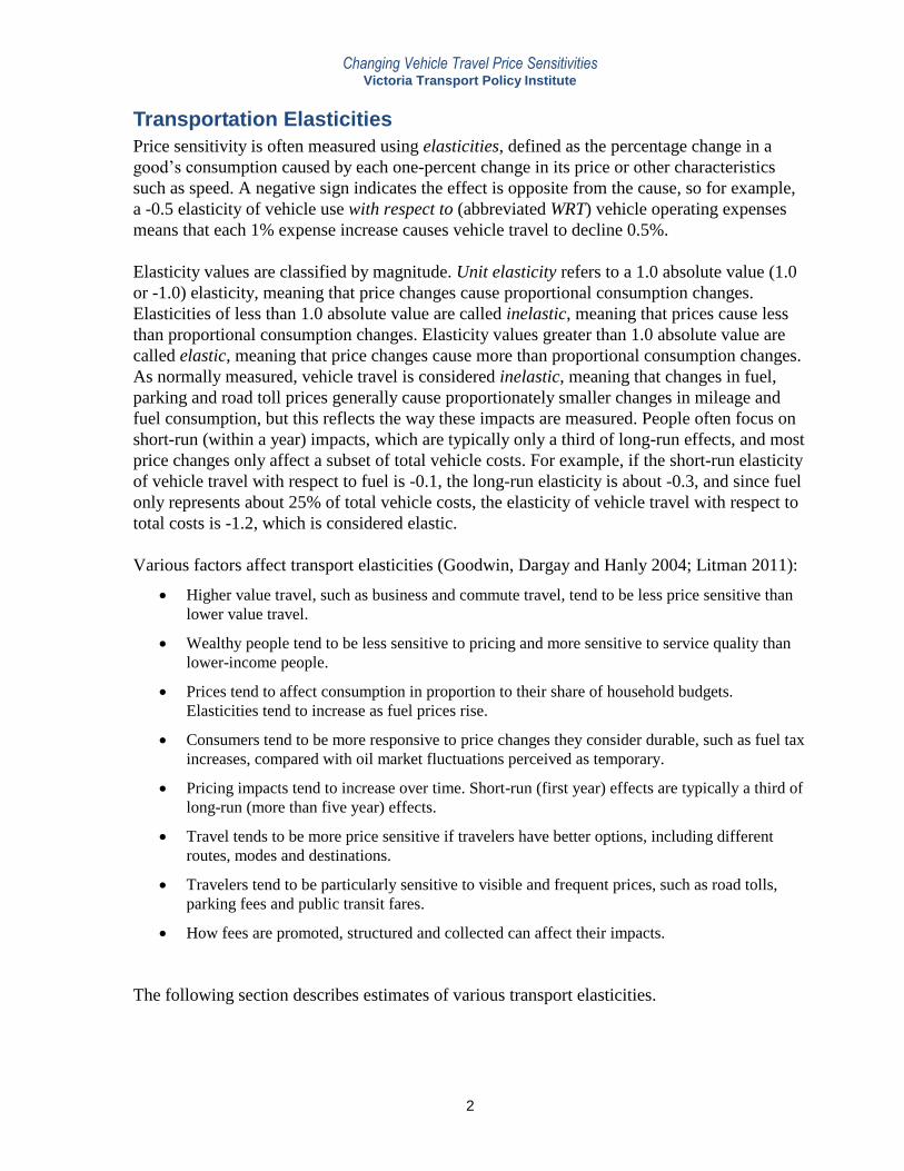
Table 1 Transportation Price Reforms (VTPI 2010)
Name Description
Road pricing Road tolls and mileage fees with rates that increase under congested conditions.
Parking pricing Direct user financing of parking facilities with rates that vary by time and location.
Fuel pricing Reduced subsidies and increased fuel taxes.
Distance-based pricing Basing insurance and registration fees directly on the amount a vehicle is driven.
Transport pricing reforms are advocated to achieve various planning objectives including traffic and
parking congestion reductions, traffic safety, energy conservation and emission reductions.
Many people are skeptical. They believe that pricing has little effect on travel activity so pricing
reforms are ineffective and harmful to consumers and the economy, and other strategies are more
effective at achieving planning objectives. A key factor in this analysis is the price sensitivity of
transport, that is, the amount that price changes affect travel activity and fuel consumption,
measured as elasticities: the percentage change in consumption caused by a percentage change in
price.
Lower elasticities (price changes cause relatively small changes in consumption) imply that
pricing reforms have small impacts and benefits, and that consumers lack viable alternatives
and so are significantly burdened by price increases (what economists call a loss of consumer
surplus). In addition, low price elasticities imply that rebound effects (additional vehicle travel
that results from increased fuel economy1) are small, so regulations and incentives that
encourage the purchase of more fuel efficient vehicles are effective at reducing total fuel and
emissions. Conversely, high elasticities (price changes cause relatively large changes in
consumption) imply that price reforms are relatively effective and beneficial, that consumers
can reduce vehicle travel and fuel consumption with minimal harm, and rebound effects are
large so regulations and incentives that encourage vehicle fuel efficiency are less effective and
cause large increases in external costs.
Some research indicates that vehicle travel became less price sensitive during the last quarter
of the Twentieth Century, but there is growing evidence that the very low elasticities reported
during that time period were an anomaly, reflecting unique demographic and economic
conditions, and transport elasticities are increasing to more normal levels. This report explores
these issues. It discusses the concepts of price elasticities and rebound effects, reviews
information on vehicle travel and fuel price elasticities, examines evidence of changes in price
elasticity values, and discusses policy implications.
1 Fuel economy refers to the amount of fuel used per vehicle-mile or –kilometer.
Changing Vehicle Travel Price Sensitivities Victoria Transport Policy Institute
2
Transportation Elasticities
Price sensitivity is often measured using elasticities, defined as the percentage change in a
good’s consumption caused by each one-percent change in its price or other characteristics
such as speed. A negative sign indicates the effect is opposite from the cause, so for example,
a -0.5 elasticity of vehicle use with respect to (abbreviated WRT) vehicle operating expenses
means that each 1% expense increase causes vehicle travel to decline 0.5%.
Elasticity values are classified by magnitude. Unit elasticity refers to a 1.0 absolute value (1.0
or -1.0) elasticity, meaning that price changes cause proportional consumption changes.
Elasticities of less than 1.0 absolute value are called inelastic, meaning that prices cause less
than proportional consumption changes. Elasticity values greater than 1.0 absolute value are
called elastic, meaning that price changes cause more than proportional consumption changes.
As normally measured, vehicle travel is considered inelastic, meaning that changes in fuel,
parking and road toll prices generally cause proportionately smaller changes in mileage and
fuel consumption, but this reflects the way these impacts are measured. People often focus on
short-run (within a year) impacts, which are typically only a third of long-run effects, and most
price changes only affect a subset of total vehicle costs. For example, if the short-run elasticity
of vehicle travel with respect to fuel is -0.1, the long-run elasticity is about -0.3, and since fuel
only represents about 25% of total vehicle costs, the elasticity of vehicle travel with respect to
total costs is -1.2, which is considered elastic.
Various factors affect transport elasticities (Goodwin, Dargay and Hanly 2004; Litman 2011):
Higher value travel, such as business and commute travel, tend to be less price sensitive than
lower value travel.
Wealthy people tend to be less sensitive to pricing and more sensitive to service quality than
lower-income people.
Prices tend to affect consumption in proportion to their share of household budgets.
Elasticities tend to increase as fuel prices rise.
Consumers tend to be more responsive to price changes they consider durable, such as fuel tax
increases, compared with oil market fluctuations perceived as temporary.
Pricing impacts tend to increase over time. Short-run (first year) effects are typically a third of
long-run (more than five year) effects.
Travel tends to be more price sensitive if travelers have better options, including different
routes, modes and destinations.
Travelers tend to be particularly sensitive to visible and frequent prices, such as road tolls,
parking fees and public transit fares.
How fees are promoted, structured and collected can affect their impacts.
The following section describes estimates of various transport elasticities.
Changing Vehicle Travel Price Sensitivities Victoria Transport Policy Institute
3
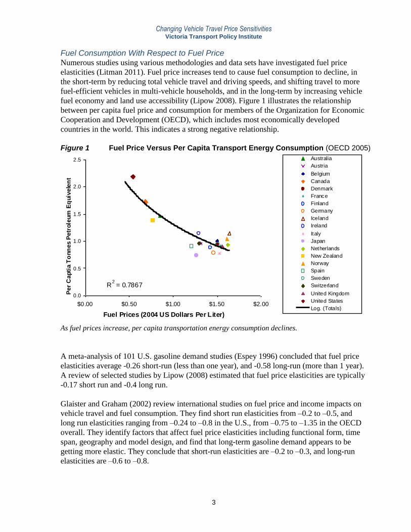
Fuel Consumption With Respect to Fuel Price Numerous studies using various methodologies and data sets have investigated fuel price
elasticities (Litman 2011). Fuel price increases tend to cause fuel consumption to decline, in
the short-term by reducing total vehicle travel and driving speeds, and shifting travel to more
fuel-efficient vehicles in multi-vehicle households, and in the long-term by increasing vehicle
fuel economy and land use accessibility (Lipow 2008). Figure 1 illustrates the relationship
between per capita fuel price and consumption for members of the Organization for Economic
Cooperation and Development (OECD), which includes most economically developed
countries in the world. This indicates a strong negative relationship.
Figure 1 Fuel Price Versus Per Capita Transport Energy Consumption (OECD 2005)
R2 = 0.7867
0.0
0.5
1.0
1.5
2.0
2.5
$0.00 $0.50 $1.00 $1.50 $2.00
Fuel Prices (2004 US Dollars Per Liter)
Per
Capti
a T
onn
es P
etr
ole
um
Eq
uiv
ele
nt
Australia
Austria
Belgium
Canada
Denmark
France
Finland
Germany
Iceland
Ireland
Italy
Japan
Netherlands
New Zealand
Norway
Spain
Sweden
Switzerland
United Kingdom
United States
Log. (Totals)
As fuel prices increase, per capita transportation energy consumption declines.
A meta-analysis of 101 U.S. gasoline demand studies (Espey 1996) concluded that fuel price
elasticities average -0.26 short-run (less than one year), and -0.58 long-run (more than 1 year).
A review of selected studies by Lipow (2008) estimated that fuel price elasticities are typically
-0.17 short run and -0.4 long run.
Glaister and Graham (2002) review international studies on fuel price and income impacts on
vehicle travel and fuel consumption. They find short run elasticities from –0.2 to –0.5, and
long run elasticities ranging from –0.24 to –0.8 in the U.S., from –0.75 to –1.35 in the OECD
overall. They identify factors that affect fuel price elasticities including functional form, time
span, geography and model design, and find that long-term gasoline demand appears to be
getting more elastic. They conclude that short-run elasticities are –0.2 to –0.3, and long-run
elasticities are –0.6 to –0.8.
Changing Vehicle Travel Price Sensitivities Victoria Transport Policy Institute
4
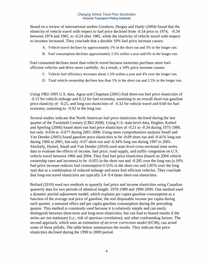
Based on a review of international studies Goodwin, Dargay and Hanly (2004) found that the
elasticity of vehicle travel with respect to fuel price declined from -0.54 prior to 1974, -0.34
between 1974 and 1981, to -0.24 after 1981, while the elasticity of vehicle travel with respect
to incomes increased. They conclude that a durable 10% fuel price increase causes:
A. Vehicle travel declines by approximately 1% in the short run and 3% in the longer run.
B. Fuel consumption declines approximately 2.5% within a year and 6% in the longer run.
Fuel consumed declines more than vehicle travel because motorists purchase more fuel-
efficient vehicles and drive more carefully. As a result, a 10% price increase causes:
C. Vehicle fuel efficiency increases about 1.5% within a year and 4% over the longer run.
D. Total vehicle ownership declines less than 1% in the short run and 2.5% in the longer run.
Using 1982-1995 U.S. data, Agras and Chapman (2001) find short-run fuel price elasticities of
–0.15 for vehicle mileage and 0.12 for fuel economy, summing to an overall short-run gasoline
price elasticity of –0.25, and long-run elasticities of –0.32 for vehicle travel and 0.60 for fuel
economy, summing to –0.92 in the long run.
Several studies indicate that North American fuel price elasticities declined during the last
quarter of the Twentieth Century (CBO 2008). Using U.S. state-level data, Hughes, Knittel
and Sperling (2006) found short-run fuel price elasticities of -0.21 to -0.34 during 1975-1980,
but only -0.034 to -0.077 during 2001-2006. Using more comprehensive analysis Small and
Van Dender (2005) found gasoline price elasticities to be -0.09 short run and -0.41% long run
during 1966 to 2001, but only -0.07 short run and -0.34% long run during 1997 to 2001.
Similarly, Hymel, Small and Van Dender (2010) used state-level cross-sectional time series
data to evaluate the effects of income, fuel price, road supply, and traffic congestion on U.S.
vehicle travel between 1966 and 2004. They find fuel price elasticities (based on 2004 vehicle
ownership rates and incomes) to be -0.055 in the short run and -0.285 over the long run (a 10%
fuel price increase reduces fuel consumption 0.55% in the short run and 2.85% over the long
run) due to a combination of reduced mileage and more fuel efficient vehicles. They conclude
that long-run travel elasticities are typically 3.4–9.4 times short-run elasticities.
Boilard (2010) used two methods to quantify fuel price and income elasticities using Canadian
quarterly data for two periods of identical length: 1970-1989 and 1990-2009. One method used
a dynamic partial adjustment model, which explains per capita gasoline consumption as a
function of the average real price of gasoline, the real disposable income per capita during
each quarter, a seasonal effect and per capita gasoline consumption during the preceding
quarter. This method is commonly used because it is relatively simple and can easily
distinguish between short-term and long-term elasticities, but can lead to biased results if the
series are not stationary (i.e., risk of spurious correlation), and other confounding factors. The
second approach, which uses an estimation of an error correction model (ECM), can avoid
some of these pitfalls. The table below summarizes the results. They indicate that price
elasticities declined during the 1990 to 2009 period.

Changing Vehicle Travel Price Sensitivities Victoria Transport Policy Institute
5
Table 2 Canadian Fuel Price and Income Elasticities (Boilard 2010)
Approach Elasticity 1970-1989 1990-2009
Short Term Long Term Short Term Long Term
Dynamic Model Price -0.093 -0.762 -0.091 -0.256
Income 0.046 0.377 0.249 0.699
Cointegration Price -0.193 -0.450 -0.046 -0.085
Model Income 0.209 0.428 0.169 0.423
This table summaries short- and long-term fuel price and income elasticities in Canada.
These low values may reflect unique factors during that period, including growing per capita
vehicle ownership, employement and incomes, combined with declining real fuel prices which
reduced fuel prices relative to incomes, plus highway expansion and dispersed development
patterns (Litman 2006). More recent studies suggest that fuel price elasticities began to
increase after about 2005 (CERA 2006). Komanoff (2008) estimated the short-run U.S. fuel
price elasticity reached a low of -0.04 in 2004, but increased to -0.08 in 2005, -0.12 in 2006,
-0.16 in 2007 and -0.29 in 2011. Brand (2009) found that the 20% U.S. fuel price increase
between 2007 and 2008 caused fuel consumption to decline 4.0%, a short-run price elasticity
of -0.13, or about -0.17 accounting for population and economic growth during that period.
Li, Linn and Muehlegger (2011) used U.S. gasoline consumption, vehicle travel, vehicle
ownership, and new vehicle purchase data to evaluate how price changes affected transport
activity and fuel consumption between 1968 and 2008. They find that fuel tax increases, which
are considered durable, have a greater effect on fuel consumption than market fluctuations.
They estimate the elasticity of gasoline demand with respect to fuel price is -0.235, with
greater elasticities for taxes than tax-exclusive oil price fluctuations. This suggests that the
decline in fuel price elasticities between 1970 and 2000 may partly reflect the decline in the
tax share of fuel prices, a factor generally overlooked elasticity studies. This suggests that
increases in motor vehicle operating costs that consumers consider durable (fuel taxes, road
tolls, parking fees and distance-based insurance and registration fees) are likely to cause much
greater reductions in vehicle travel and fuel consumption than indicated by conventional
models which use elasticity value based on responses to price changes that consumers
considered temporary. Spiller and Stephens (2012) developed a comprehensive model using
data from the 2009 National Household Travel Survey, U.S. Census, and monthly state-level
gasoline prices to estimate household-level fuel price elasticities. They found the mean short-
run price elasticity of gasoline to be -0.67, with significant variations by location and income.
Table 3 summarizes these studies. They vary significantly in scope and methodology. Many
older studies used relatively simple models, more recent studies tend to account for more
demographic, economic and geographic factors. These studies indicate that fuel price
elasticities declined during the last quarter of the Twentieth Century, under -0.1 short-run and
under -0.4 long-run (Small and Van Dender 2005; Hymel, Small and Van Dender 2010), but
higher elasticities have been measured during the first decade of the Twenty-first Century,
between -0.1 and -0.2 short-run, and -0.2 to -0.3 medium-run (Boilard 2010; Komanoff 2008-
2011; Spiller and Stephens 2012).
Changing Vehicle Travel Price Sensitivities Victoria Transport Policy Institute
6
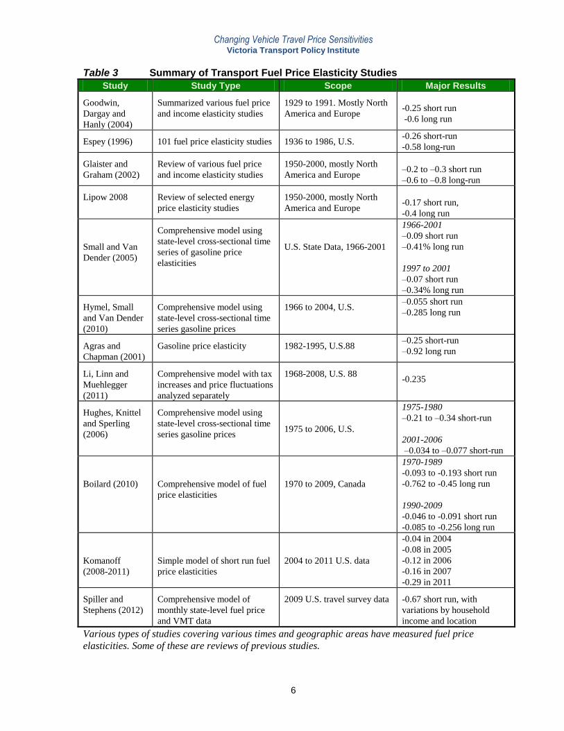
Table 3 Summary of Transport Fuel Price Elasticity Studies
Study Study Type Scope Major Results
Goodwin,
Dargay and
Hanly (2004)
Summarized various fuel price
and income elasticity studies
1929 to 1991. Mostly North
America and Europe
-0.25 short run
-0.6 long run
Espey (1996) 101 fuel price elasticity studies 1936 to 1986, U.S. -0.26 short-run
-0.58 long-run
Glaister and
Graham (2002)
Review of various fuel price
and income elasticity studies
1950-2000, mostly North
America and Europe
–0.2 to –0.3 short run
–0.6 to –0.8 long-run
Lipow 2008 Review of selected energy
price elasticity studies
1950-2000, mostly North
America and Europe
-0.17 short run,
-0.4 long run
Small and Van
Dender (2005)
Comprehensive model using
state-level cross-sectional time
series of gasoline price
elasticities
U.S. State Data, 1966-2001
1966-2001
–0.09 short run
–0.41% long run
1997 to 2001
–0.07 short run
–0.34% long run
Hymel, Small
and Van Dender
(2010)
Comprehensive model using
state-level cross-sectional time
series gasoline prices
1966 to 2004, U.S. –0.055 short run
–0.285 long run
Agras and
Chapman (2001)
Gasoline price elasticity 1982-1995, U.S.88 –0.25 short-run
–0.92 long run
Li, Linn and
Muehlegger
(2011)
Comprehensive model with tax
increases and price fluctuations
analyzed separately
1968-2008, U.S. 88
-0.235
Hughes, Knittel
and Sperling
(2006)
Comprehensive model using
state-level cross-sectional time
series gasoline prices
1975 to 2006, U.S.
1975-1980
–0.21 to –0.34 short-run
2001-2006
–0.034 to –0.077 short-run
Boilard (2010)
Comprehensive model of fuel
price elasticities
1970 to 2009, Canada
1970-1989
-0.093 to -0.193 short run
-0.762 to -0.45 long run
1990-2009
-0.046 to -0.091 short run
-0.085 to -0.256 long run
Komanoff
(2008-2011)
Simple model of short run fuel
price elasticities
2004 to 2011 U.S. data
-0.04 in 2004
-0.08 in 2005
-0.12 in 2006
-0.16 in 2007
-0.29 in 2011
Spiller and
Stephens (2012)
Comprehensive model of
monthly state-level fuel price
and VMT data
2009 U.S. travel survey data -0.67 short run, with
variations by household
income and location
Various types of studies covering various times and geographic areas have measured fuel price
elasticities. Some of these are reviews of previous studies.
Changing Vehicle Travel Price Sensitivities Victoria Transport Policy Institute
7
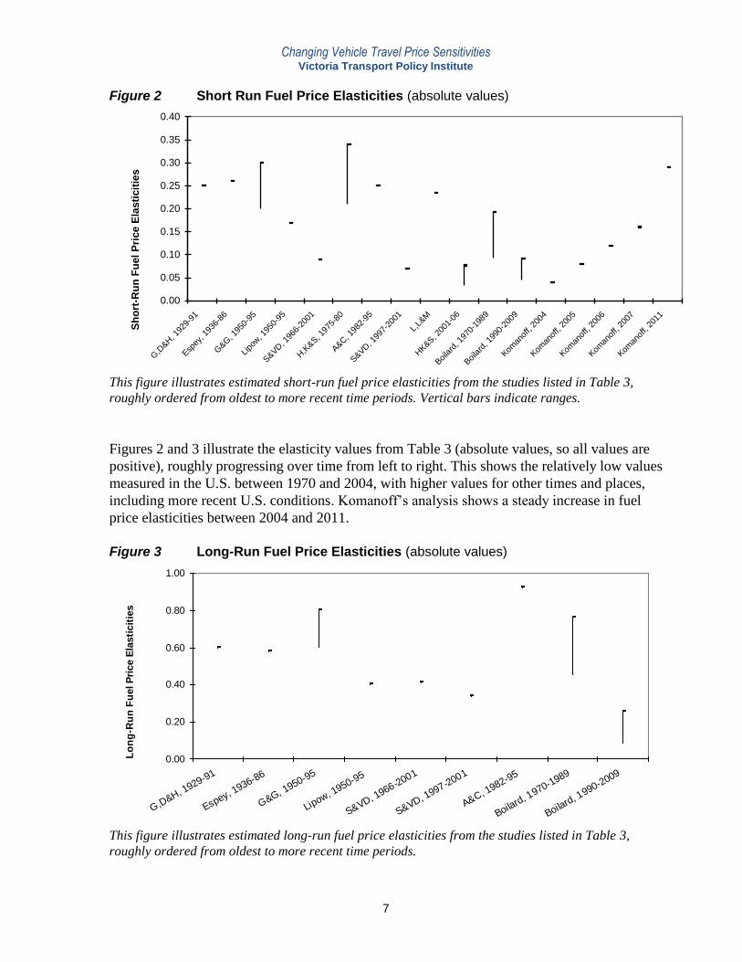
Figure 2 Short Run Fuel Price Elasticities (absolute values)
0.00
0.05
0.10
0.15
0.20
0.25
0.30
0.35
0.40
G,D
&H, 1
929-
91
Espey
, 193
6-86
G&G
, 195
0-95
Lipo
w, 1
950-
95
S&VD
, 196
6-20
01
H,K
&S, 1
975-
80
A&C, 1
982-
95
S&VD
, 199
7-20
01
L,L&
M
HK&S
, 200
1-06
Boilard
, 197
0-19
89
Boilard
, 199
0-20
09
Koman
off,
2004
Koman
off,
2005
Koman
off,
2006
Koman
off,
2007
Koman
off,
2011
Sh
ort
-Ru
n F
uel P
rice E
lasti
cit
ies
This figure illustrates estimated short-run fuel price elasticities from the studies listed in Table 3,
roughly ordered from oldest to more recent time periods. Vertical bars indicate ranges.
Figures 2 and 3 illustrate the elasticity values from Table 3 (absolute values, so all values are
positive), roughly progressing over time from left to right. This shows the relatively low values
measured in the U.S. between 1970 and 2004, with higher values for other times and places,
including more recent U.S. conditions. Komanoff’s analysis shows a steady increase in fuel
price elasticities between 2004 and 2011.
Figure 3 Long-Run Fuel Price Elasticities (absolute values)
0.00
0.20
0.40
0.60
0.80
1.00
G,D&H, 1
929-91
Espey, 1936-86
G&G, 1950-95
Lipow, 1950-95
S&VD, 1966-2001
S&VD, 1997-2001
A&C, 1982-95
Boilard, 1
970-1989
Boilard, 1
990-2009
Lo
ng
-Ru
n F
uel P
rice E
lasti
cit
ies
This figure illustrates estimated long-run fuel price elasticities from the studies listed in Table 3,
roughly ordered from oldest to more recent time periods.
Changing Vehicle Travel Price Sensitivities Victoria Transport Policy Institute
8
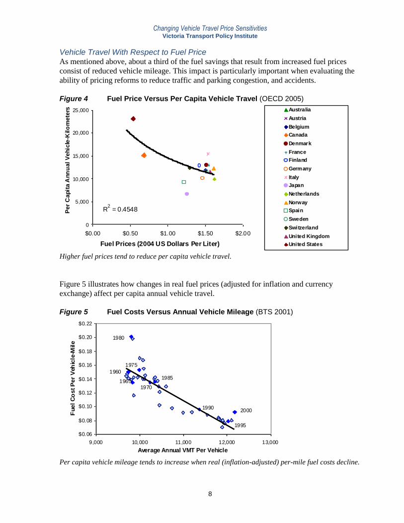
Vehicle Travel With Respect to Fuel Price As mentioned above, about a third of the fuel savings that result from increased fuel prices
consist of reduced vehicle mileage. This impact is particularly important when evaluating the
ability of pricing reforms to reduce traffic and parking congestion, and accidents.
Figure 4 Fuel Price Versus Per Capita Vehicle Travel (OECD 2005)
R2 = 0.4548
0
5,000
10,000
15,000
20,000
25,000
$0.00 $0.50 $1.00 $1.50 $2.00
Fuel Prices (2004 US Dollars Per Liter)
Per
Capit
a A
nn
ual V
ehic
le-K
ilo
mete
rs Australia
Austria
Belgium
Canada
Denmark
France
Finland
Germany
Italy
Japan
Netherlands
Norway
Spain
Sweden
Switzerland
United Kingdom
United States
Higher fuel prices tend to reduce per capita vehicle travel.
Figure 5 illustrates how changes in real fuel prices (adjusted for inflation and currency
exchange) affect per capita annual vehicle travel.
Figure 5 Fuel Costs Versus Annual Vehicle Mileage (BTS 2001)
$0.06
$0.08
$0.10
$0.12
$0.14
$0.16
$0.18
$0.20
$0.22
9,000 10,000 11,000 12,000 13,000
Average Annual VMT Per Vehicle
Fuel C
ost P
er
Veh
icle
-Mile
1960
19651970
1975
1980
1985
1990
1995
2000
Per capita vehicle mileage tends to increase when real (inflation-adjusted) per-mile fuel costs decline.
Changing Vehicle Travel Price Sensitivities Victoria Transport Policy Institute
9
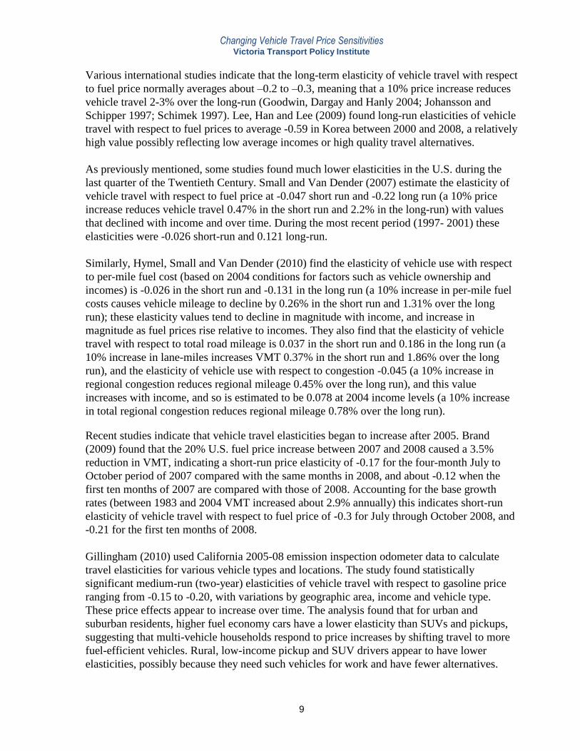
Various international studies indicate that the long-term elasticity of vehicle travel with respect
to fuel price normally averages about –0.2 to –0.3, meaning that a 10% price increase reduces
vehicle travel 2-3% over the long-run (Goodwin, Dargay and Hanly 2004; Johansson and
Schipper 1997; Schimek 1997). Lee, Han and Lee (2009) found long-run elasticities of vehicle
travel with respect to fuel prices to average -0.59 in Korea between 2000 and 2008, a relatively
high value possibly reflecting low average incomes or high quality travel alternatives.
As previously mentioned, some studies found much lower elasticities in the U.S. during the
last quarter of the Twentieth Century. Small and Van Dender (2007) estimate the elasticity of
vehicle travel with respect to fuel price at -0.047 short run and -0.22 long run (a 10% price
increase reduces vehicle travel 0.47% in the short run and 2.2% in the long-run) with values
that declined with income and over time. During the most recent period (1997- 2001) these
elasticities were -0.026 short-run and 0.121 long-run.
Similarly, Hymel, Small and Van Dender (2010) find the elasticity of vehicle use with respect
to per-mile fuel cost (based on 2004 conditions for factors such as vehicle ownership and
incomes) is -0.026 in the short run and -0.131 in the long run (a 10% increase in per-mile fuel
costs causes vehicle mileage to decline by 0.26% in the short run and 1.31% over the long
run); these elasticity values tend to decline in magnitude with income, and increase in
magnitude as fuel prices rise relative to incomes. They also find that the elasticity of vehicle
travel with respect to total road mileage is 0.037 in the short run and 0.186 in the long run (a
10% increase in lane-miles increases VMT 0.37% in the short run and 1.86% over the long
run), and the elasticity of vehicle use with respect to congestion -0.045 (a 10% increase in
regional congestion reduces regional mileage 0.45% over the long run), and this value
increases with income, and so is estimated to be 0.078 at 2004 income levels (a 10% increase
in total regional congestion reduces regional mileage 0.78% over the long run).
Recent studies indicate that vehicle travel elasticities began to increase after 2005. Brand
(2009) found that the 20% U.S. fuel price increase between 2007 and 2008 caused a 3.5%
reduction in VMT, indicating a short-run price elasticity of -0.17 for the four-month July to
October period of 2007 compared with the same months in 2008, and about -0.12 when the
first ten months of 2007 are compared with those of 2008. Accounting for the base growth
rates (between 1983 and 2004 VMT increased about 2.9% annually) this indicates short-run
elasticity of vehicle travel with respect to fuel price of -0.3 for July through October 2008, and
-0.21 for the first ten months of 2008.
Gillingham (2010) used California 2005-08 emission inspection odometer data to calculate
travel elasticities for various vehicle types and locations. The study found statistically
significant medium-run (two-year) elasticities of vehicle travel with respect to gasoline price
ranging from -0.15 to -0.20, with variations by geographic area, income and vehicle type.
These price effects appear to increase over time. The analysis found that for urban and
suburban residents, higher fuel economy cars have a lower elasticity than SUVs and pickups,
suggesting that multi-vehicle households respond to price increases by shifting travel to more
fuel-efficient vehicles. Rural, low-income pickup and SUV drivers appear to have lower
elasticities, possibly because they need such vehicles for work and have fewer alternatives.

Changing Vehicle Travel Price Sensitivities Victoria Transport Policy Institute
10
Li, Linn and Muehlegger (2011) find that in the U.S. between 1968 and 2008 the elasticity of
vehicle travel with respect to gasoline prices ranged from -0.24 to -0.34, depending on time
period and model specifications, with no significant difference between taxes and other price
changes. NCHRP (2006) and Williams-Derry (2011) summarizes research indicating that
motorists are more sensitive to road tolls than most models predict. Fuel prices influence
household location decisions in ways that can affect long-run impacts on travel activity.
Molloy and Hui Shan (2011) found that a 10% gasoline price increase reduces demand for
housing in locations with a long average commutes by 10% after a 4-year lag. Spiller and
Stephens (2012) used data from the 2009 National Household Travel Survey, the U.S. Census,
and monthly state-level gasoline prices to estimate vehicle travel elasticities. They found the
mean short-run household-level elasticity of VMT to fuel price to be -0.67, with significant
variations by location and income.
Table 4 summarizes these studies’ results. As with the fuel price elasticity data, analysis
quality varies. The results indicate that vehicle travel price sensitivities declined during the last
quarter of the Twentieth Century, with elasticities below –0.1 short-run and –0.2 long-run
(Small and Van Dender 2010; Hymel, Small and Van Dender 2010), but more recent studies
based on data after 2000 indicate higher elasticities,–0.1 to –0.2 short-run, and –0.2 to -0.3
long-run (Brand 2009; Gillingham 2010; Spiller and Stephens 2012).
Changing Vehicle Travel Price Sensitivities Victoria Transport Policy Institute
11
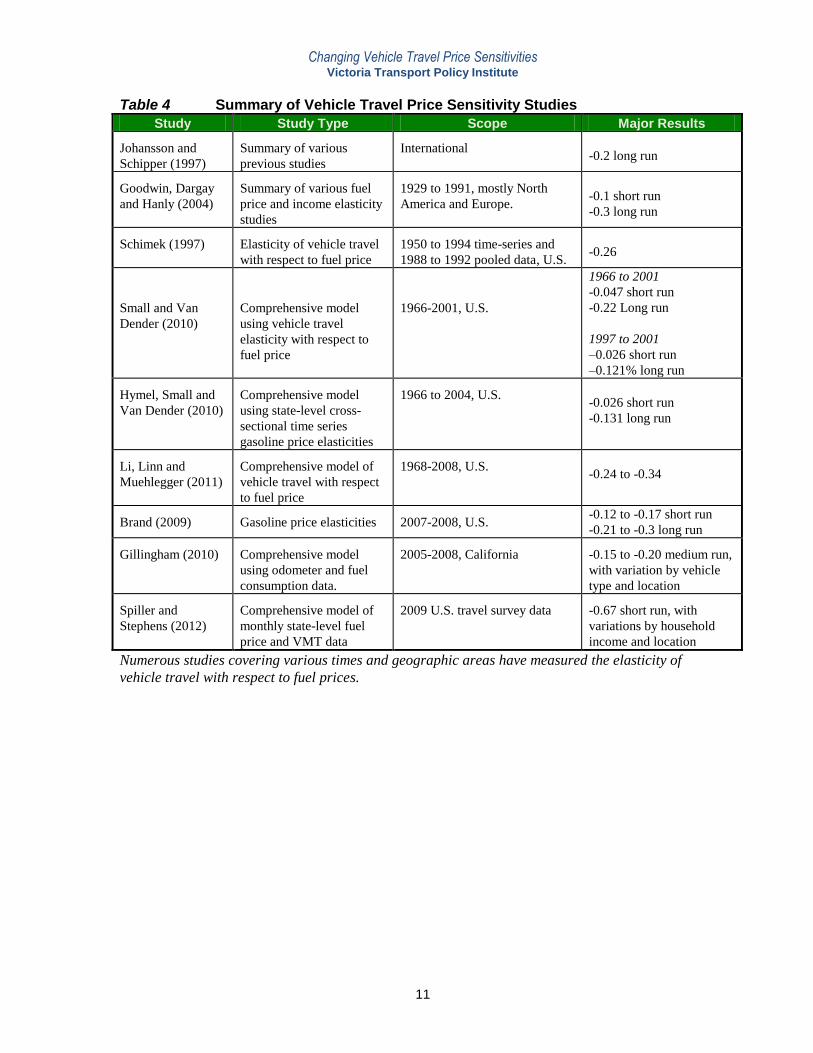
Table 4 Summary of Vehicle Travel Price Sensitivity Studies
Study Study Type Scope Major Results
Johansson and
Schipper (1997)
Summary of various
previous studies
International
-0.2 long run
Goodwin, Dargay
and Hanly (2004)
Summary of various fuel
price and income elasticity
studies
1929 to 1991, mostly North
America and Europe.
-0.1 short run
-0.3 long run
Schimek (1997) Elasticity of vehicle travel
with respect to fuel price
1950 to 1994 time-series and
1988 to 1992 pooled data, U.S.
-0.26
Small and Van
Dender (2010)
Comprehensive model
using vehicle travel
elasticity with respect to
fuel price
1966-2001, U.S.
1966 to 2001
-0.047 short run
-0.22 Long run
1997 to 2001
–0.026 short run
–0.121% long run
Hymel, Small and
Van Dender (2010)
Comprehensive model
using state-level cross-
sectional time series
gasoline price elasticities
1966 to 2004, U.S.
-0.026 short run
-0.131 long run
Li, Linn and
Muehlegger (2011)
Comprehensive model of
vehicle travel with respect
to fuel price
1968-2008, U.S.
-0.24 to -0.34
Brand (2009) Gasoline price elasticities 2007-2008, U.S. -0.12 to -0.17 short run
-0.21 to -0.3 long run
Gillingham (2010) Comprehensive model
using odometer and fuel
consumption data.
2005-2008, California -0.15 to -0.20 medium run,
with variation by vehicle
type and location
Spiller and
Stephens (2012)
Comprehensive model of
monthly state-level fuel
price and VMT data
2009 U.S. travel survey data -0.67 short run, with
variations by household
income and location
Numerous studies covering various times and geographic areas have measured the elasticity of
vehicle travel with respect to fuel prices.
Changing Vehicle Travel Price Sensitivities Victoria Transport Policy Institute
12
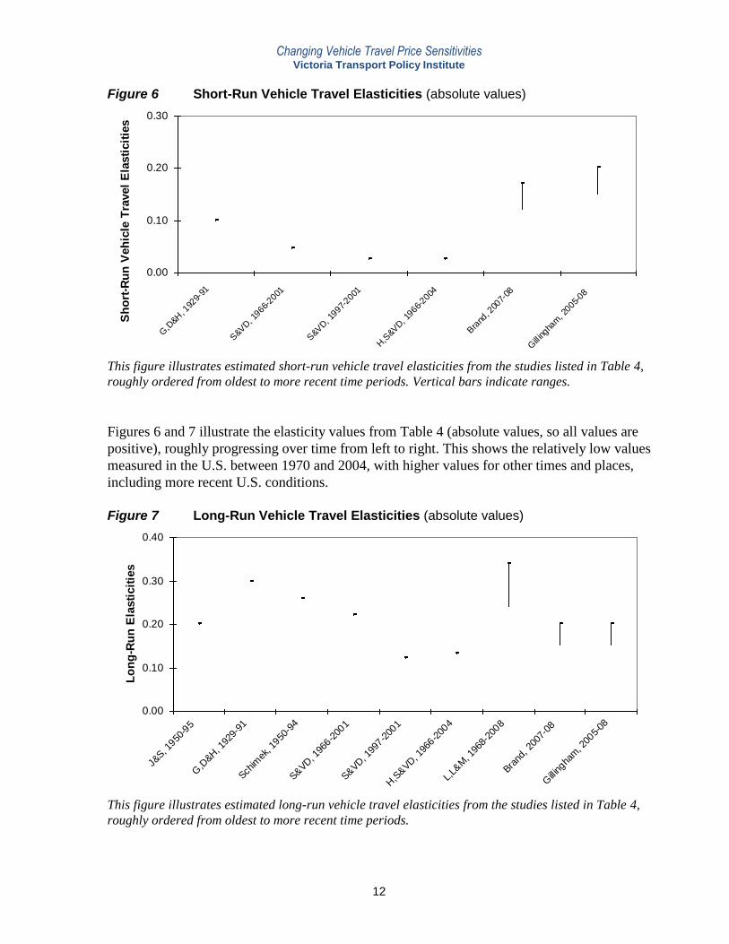
Figure 6 Short-Run Vehicle Travel Elasticities (absolute values)
0.00
0.10
0.20
0.30
G,D
&H, 1
929-
91
S&V
D, 1
966-2001
S&V
D, 1
997-2001
H,S
&VD, 1
966-2004
Bra
nd, 2
007-
08
Gillingha
m, 2
005-08
Sh
ort
-Ru
n V
eh
icle
Tra
vel
Ela
sti
cit
ies
This figure illustrates estimated short-run vehicle travel elasticities from the studies listed in Table 4,
roughly ordered from oldest to more recent time periods. Vertical bars indicate ranges.
Figures 6 and 7 illustrate the elasticity values from Table 4 (absolute values, so all values are
positive), roughly progressing over time from left to right. This shows the relatively low values
measured in the U.S. between 1970 and 2004, with higher values for other times and places,
including more recent U.S. conditions.
Figure 7 Long-Run Vehicle Travel Elasticities (absolute values)
0.00
0.10
0.20
0.30
0.40
J&S, 1
950-9
5
G,D
&H, 1
929-
91
Schim
ek, 1
950-9
4
S&VD
, 196
6-200
1
S&VD
, 199
7-200
1
H,S
&VD
, 196
6-200
4
L,L&
M, 1
968-
2008
Brand
, 200
7-08
Gilli
ngha
m, 2
005-
08
Lo
ng
-Ru
n E
lasti
cit
ies
This figure illustrates estimated long-run vehicle travel elasticities from the studies listed in Table 4,
roughly ordered from oldest to more recent time periods.
Changing Vehicle Travel Price Sensitivities Victoria Transport Policy Institute
13
Discussion
The transport elasticity changes identified here can be explained by various demographic and
economic factors that affect vehicle travel demands, including ages, employment rates and
incomes, fuel prices, transport options and land use development. During the Twentieth
Century these factors tended to increase vehicle travel demand, but recent trends are reducing
travel demands, which tends to increase fuel and vehicle travel elasticities (Litman 2006).
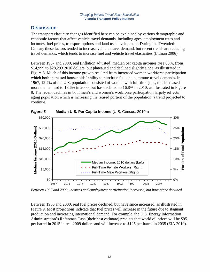
Between 1967 and 2000, real (inflation adjusted) median per capita incomes rose 88%, from
$14,999 to $28,293 2010 dollars, but plateaued and declined slightly since, as illustrated in
Figure 3. Much of this income growth resulted from increased women workforce participation
which both increased households’ ability to purchase fuel and commute travel demands. In
1967, 12.4% of the U.S. population consisted of women with full-time jobs, this increased
more than a third to 18.6% in 2000, but has declined to 16.8% in 2010, as illustrated in Figure
8. The recent declines in both men’s and women’s workforce participation largely reflects
aging population which is increasing the retired portion of the population, a trend projected to
continue.
Figure 8 Median U.S. Per Capita Income (U.S. Census, 2010a)
$0
$5,000
$10,000
$15,000
$20,000
$25,000
$30,000
1967 1972 1977 1982 1987 1992 1997 2002 2007
Med
ian
In
co
me (
2010 D
ollars
)
0%
5%
10%
15%
20%
25%
30%
Po
rtio
n o
f T
ota
l P
op
ula
tio
n
Median Income, 2010 dollars (Left)
Full-Time Female Workers (Right)
Full-Time Male Workers (Right)
Between 1967 and 2000, incomes and employment participation increased, but have since declined.
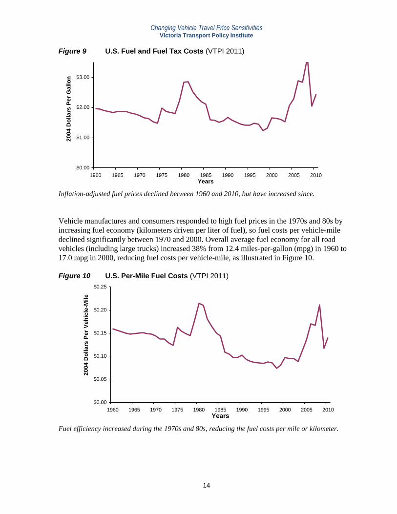
Between 1960 and 2000, real fuel prices declined, but have since increased, as illustrated in
Figure 9. Most projections indicate that fuel prices will increase in the future due to stagnant
production and increasing international demand. For example, the U.S. Energy Information
Administration’s Reference Case (their best estimate) predicts that world oil prices will be $95
per barrel in 2015 in real 2009 dollars and will increase to $125 per barrel in 2035 (EIA 2010).
Changing Vehicle Travel Price Sensitivities Victoria Transport Policy Institute
14
Figure 9 U.S. Fuel and Fuel Tax Costs (VTPI 2011)
$0.00
$1.00
$2.00
$3.00
1960 1965 1970 1975 1980 1985 1990 1995 2000 2005 2010
Years
20
04
Do
lla
rs P
er
Ga
llo
n
Inflation-adjusted fuel prices declined between 1960 and 2010, but have increased since.
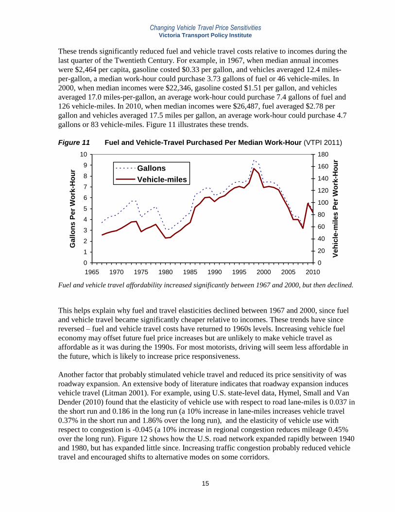
Vehicle manufactures and consumers responded to high fuel prices in the 1970s and 80s by
increasing fuel economy (kilometers driven per liter of fuel), so fuel costs per vehicle-mile
declined significantly between 1970 and 2000. Overall average fuel economy for all road
vehicles (including large trucks) increased 38% from 12.4 miles-per-gallon (mpg) in 1960 to
17.0 mpg in 2000, reducing fuel costs per vehicle-mile, as illustrated in Figure 10.
Figure 10 U.S. Per-Mile Fuel Costs (VTPI 2011)
$0.00
$0.05
$0.10
$0.15
$0.20
$0.25
1960 1965 1970 1975 1980 1985 1990 1995 2000 2005 2010
Years
20
04
Do
lla
rs P
er
Ve
hic
le-M
ile
Fuel efficiency increased during the 1970s and 80s, reducing the fuel costs per mile or kilometer.
Changing Vehicle Travel Price Sensitivities Victoria Transport Policy Institute
15
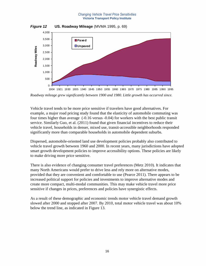
These trends significantly reduced fuel and vehicle travel costs relative to incomes during the
last quarter of the Twentieth Century. For example, in 1967, when median annual incomes
were $2,464 per capita, gasoline costed $0.33 per gallon, and vehicles averaged 12.4 miles-
per-gallon, a median work-hour could purchase 3.73 gallons of fuel or 46 vehicle-miles. In
2000, when median incomes were $22,346, gasoline costed $1.51 per gallon, and vehicles
averaged 17.0 miles-per-gallon, an average work-hour could purchase 7.4 gallons of fuel and
126 vehicle-miles. In 2010, when median incomes were $26,487, fuel averaged $2.78 per
gallon and vehicles averaged 17.5 miles per gallon, an average work-hour could purchase 4.7
gallons or 83 vehicle-miles. Figure 11 illustrates these trends.
Figure 11 Fuel and Vehicle-Travel Purchased Per Median Work-Hour (VTPI 2011)
0
1
2
3
4
5
6
7
8
9
10
1965 1970 1975 1980 1985 1990 1995 2000 2005 2010
Gall
on
s P
er
Wo
rk-H
ou
r
0
20
40
60
80
100
120
140
160
180
Veh
icle
-mil
es P
er
Wo
rk-H
ou
r
Gallons
Vehicle-miles
Fuel and vehicle travel affordability increased significantly between 1967 and 2000, but then declined.
This helps explain why fuel and travel elasticities declined between 1967 and 2000, since fuel
and vehicle travel became significantly cheaper relative to incomes. These trends have since
reversed – fuel and vehicle travel costs have returned to 1960s levels. Increasing vehicle fuel
economy may offset future fuel price increases but are unlikely to make vehicle travel as
affordable as it was during the 1990s. For most motorists, driving will seem less affordable in
the future, which is likely to increase price responsiveness.
Another factor that probably stimulated vehicle travel and reduced its price sensitivity of was
roadway expansion. An extensive body of literature indicates that roadway expansion induces
vehicle travel (Litman 2001). For example, using U.S. state-level data, Hymel, Small and Van
Dender (2010) found that the elasticity of vehicle use with respect to road lane-miles is 0.037 in
the short run and 0.186 in the long run (a 10% increase in lane-miles increases vehicle travel
0.37% in the short run and 1.86% over the long run), and the elasticity of vehicle use with
respect to congestion is -0.045 (a 10% increase in regional congestion reduces mileage 0.45%
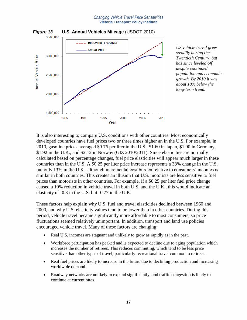
over the long run). Figure 12 shows how the U.S. road network expanded rapidly between 1940
and 1980, but has expanded little since. Increasing traffic congestion probably reduced vehicle
travel and encouraged shifts to alternative modes on some corridors.
Changing Vehicle Travel Price Sensitivities Victoria Transport Policy Institute
16
Figure 12 US. Roadway Mileage (MVMA 1995, p. 69)
0
500
1,000
1,500
2,000
2,500
3,000
3,500
4,000
1904 1921 1930 1935 1940 1945 1950 1955 1960 1965 1970 1975 1980 1985 1990 1995
Road
way M
iles
Paved
Unpaved
Roadway mileage grew significantly between 1900 and 1980. Little growth has occurred since.
Vehicle travel tends to be more price sensitive if travelers have good alternatives. For
example, a major road pricing study found that the elasticity of automobile commuting was
four times higher than average (-0.16 versus -0.04) for workers with the best public transit
service. Similarly Guo, et al. (2011) found that given financial incentives to reduce their
vehicle travel, households in denser, mixed use, transit-accessible neighborhoods responded
significantly more than comparable households in automobile dependent suburbs.
Dispersed, automobile-oriented land use development policies probably also contributed to
vehicle travel growth between 1960 and 2000. In recent years, many jurisdictions have adopted
smart growth development policies to improve accessibility options. These policies are likely
to make driving more price sensitive.
There is also evidence of changing consumer travel preferences (Metz 2010). It indicates that
many North Americans would prefer to drive less and rely more on alternative modes,
provided that they are convenient and comfortable to use (Pearce 2011). There appears to be
increased political support for policies and investments to improve alternative modes and
create more compact, multi-modal communities. This may make vehicle travel more price
sensitive if changes in prices, preferences and policies have synergistic effects.
As a result of these demographic and economic trends motor vehicle travel demand growth
slowed after 2000 and stopped after 2007. By 2010, total motor vehicle travel was about 10%
below the trend line, as indicated in Figure 13.
Changing Vehicle Travel Price Sensitivities Victoria Transport Policy Institute
17
Figure 13 U.S. Annual Vehicles Mileage (USDOT 2010)
US vehicle travel grew
steadily during the
Twentieth Century, but
has since leveled off
despite continued
population and economic
growth. By 2010 it was
about 10% below the
long-term trend.
It is also interesting to compare U.S. conditions with other countries. Most economically
developed countries have fuel prices two or three times higher an in the U.S. For example, in
2010, gasoline prices averaged $0.76 per liter in the U.S., $1.60 in Japan, $1.90 in Germany,
$1.92 in the U.K., and $2.12 in Norway (GIZ 2010/2011). Since elasticities are normally
calculated based on percentage changes, fuel price elasticities will appear much larger in these
countries than in the U.S. A $0.25 per liter price increase represents a 33% change in the U.S.
but only 13% in the U.K., although incremental cost burden relative to consumers’ incomes is
similar in both countries. This creates an illusion that U.S. motorists are less sensitive to fuel
prices than motorists in other countries. For example, if a $0.25 per liter fuel price change
caused a 10% reduction in vehicle travel in both U.S. and the U.K., this would indicate an
elasticity of -0.3 in the U.S. but -0.77 in the U.K.
These factors help explain why U.S. fuel and travel elasticities declined between 1960 and
2000, and why U.S. elasticity values tend to be lower than in other countries. During this
period, vehicle travel became significantly more affordable to most consumers, so price
fluctuations seemed relatively unimportant. In addition, transport and land use policies
encouraged vehicle travel. Many of these factors are changing:
Real U.S. incomes are stagnant and unlikely to grow as rapidly as in the past.
Workforce participation has peaked and is expected to decline due to aging population which
increases the number of retirees. This reduces commuting, which tend to be less price
sensitive than other types of travel, particularly recreational travel common to retirees.
Real fuel prices are likely to increase in the future due to declining production and increasing
worldwide demand.
Roadway networks are unlikely to expand significantly, and traffic congestion is likely to
continue at current rates.
Changing Vehicle Travel Price Sensitivities Victoria Transport Policy Institute
18
Current transport and land use policies are likely to improve alternative modes and encourage
more compact, multi-modal community development.
Consumers’ preferences appear to be shifting away from automobile travel and automobile-
dependent locations, to favor other modes and more compact, multi-modal communities.
Rising international oil prices may raise U.S. fuel prices relative to those in other countries.
As fuel and vehicle-travel costs increase relative to incomes, and as transport and land use
options improve so consumers have better alternatives to driving and automobile-dependent
communities, it is likely that fuel and travel price elasticities will tend to increase.
Putting Fuel Prices Into Perspective
Vehicle fuel is an inelastic good (a price change causes a proportionately smaller change in
consumption, that is, the elasticity value is less than 1.0). To understand why it is useful to put fuel
prices into perspective with respect to total vehicle costs.
Most motor vehicle monetary costs are considered fixed, including depreciation (although
depreciation increases with vehicle use this is a long-term effect that probably has little effect on
consumers’ short-term travel decisions), financing, insurance, registration fees, and residential
parking. For a typical automobile these costs total about $4,000 annually, averaging about 33¢ per
vehicle-mile. Travel time costs are also significant. If valued at $10 per hour, time costs average 33¢
per mile at 30 miles-per-hour.
Typical fuel price fluctuations (say, between $2.00 and $3.00 per gallon, which increase costs from
10¢ to 15¢ per vehicle-mile) are relatively modest compared with these other costs. This helps explain
why motorists have been relatively insensitive to typical fuel price changes: fuel was a relatively small
portion of total vehicle costs. If the long-run elasticity of vehicle travel with respect to fuel price is -
0.3 and fuel represents 25% of total vehicle costs, then the long-run elasticity of vehicle travel with
respect to total vehicle costs is actually -1.2, making vehicle travel elastic overall.
Changing Vehicle Travel Price Sensitivities Victoria Transport Policy Institute
19
Consumer Impacts
Price sensitivities indicate the value consumers place on a good and their ability to change
consumption when prices change. Low road, parking and fuel price elasticities indicate that
motorists value driving and find it difficult to reduce mileage and conserve fuel, so price
increases harm consumers. Higher elasticities indicate that consumers have less difficulty
reducing vehicle travel and fuel consumption, so price increases cause less harm to consumers.
These impacts can be quantified based on consumer surplus analysis, which can quantify the
value that consumers place on travel forgone due to higher prices, using a method known as
the rule of half, which is described in the following box.
Explanation of the “Rule of Half”
Economic theory suggests that when consumers change their travel in response to a financial
incentive, the net consumer surplus is half of their price change (called the rule of half). This takes
into account total changes in financial costs, travel time, convenience and mobility as they are
perceived by consumers.
Let’s say that the price of driving (that is, the perceived variable costs, or vehicle operating costs)
increased by 10¢ per mile, either because of an additional fee (e.g., paid parking) or a financial
reward, and as a result you reduced your annual vehicle use by 1,000 miles. You would not give up
highly valuable vehicle travel, but there are probably some vehicle-miles that you would reduce,
either by shifting to other modes, choosing closer destinations, or because the trip itself does not
seem particularly important.
These vehicle-miles forgone have an incremental value to you, the consumer, between 0¢ and 10¢. If
you consider the additional mile worth less than 0¢ (i.e., it has no value), you would not have taken it
in the first place. If it is worth between 1-9¢ per mile, a 10¢ per mile incentive will convince you to
give it up – you’d rather have the money. If the additional mile is worth more than 10¢ per mile, a
10¢ per mile incentive is inadequate to convenience you to give it up – you’ll keep driving. Of the
1,000 miles forgone, we can assume that the average net benefit to consumers (called the consumer
surplus) is the mid-point of this range, that is, 5¢ per vehicle mile. Thus, we can calculate that miles
forgone by a 10¢ per mile financial incentive have an average consumer surplus value of 5¢. A $100
increase in vehicle operating costs that reduces automobile travel by 1,000 miles imposes a net cost
to consumers of $50, while a $100 financial reward that convinces motorists to drive 1,000 miles less
provides a net benefit to consumers of $50.
Some people complicate this analysis by trying to track changes in consumer travel time,
convenience and vehicle operating costs, but that is unnecessary information. All we need to know to
determine net consumer benefits and costs is the perceived change in price, either positive or
negative, and the resulting change in consumption. All of the complex trade-offs that consumers
make between money, time, convenience and the value off mobility are incorporated.
For example, if a $1 per trip highway toll increase causes annual vehicle trips to decline from
5 million to 4 million, the reduction in consumer surplus is $4,500,000 ($1 x 4 million for the
motorists who pay the toll, plus $1 x 1 million x 0.5 for vehicle trips forgone). If the same $1
toll causes vehicle trips to decline from 5 million to 3 million, the reduction in consumer
surplus is a smaller $4,000,000 ($1 x 3 million for the motorists who pay the toll, plus $1 x 2
million x 0.5 for vehicle trips forgone).
Changing Vehicle Travel Price Sensitivities Victoria Transport Policy Institute
20
Transport pricing reforms can provide positive as well as negative consumer surplus impacts.
For example, if pay-as-you-drive vehicle insurance premiums that average 10¢ per vehicle-
mile cause affected vehicles to drive on average 1,000 fewer annual miles and save $100
annually in reduced insurance premiums, the net consumer surplus averages $50 ($0.10 x
1,000 x 0.5) per vehicle.2 Similarly, if the same price incentive causes affected vehicles to
drive 2,000 fewer annual miles and save $200 annually in reduced insurance premiums, the net
consumer surplus averages $100 ($0.10 x 2,000 x 0.5) per vehicle.
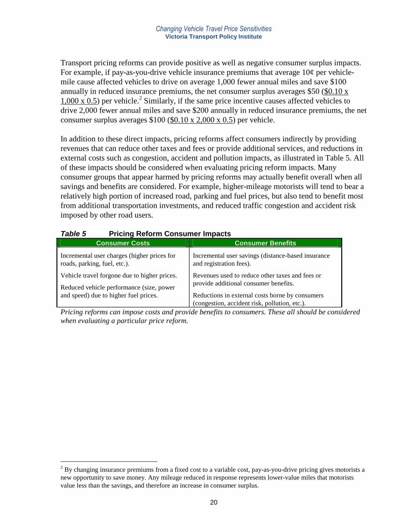
In addition to these direct impacts, pricing reforms affect consumers indirectly by providing
revenues that can reduce other taxes and fees or provide additional services, and reductions in
external costs such as congestion, accident and pollution impacts, as illustrated in Table 5. All
of these impacts should be considered when evaluating pricing reform impacts. Many
consumer groups that appear harmed by pricing reforms may actually benefit overall when all
savings and benefits are considered. For example, higher-mileage motorists will tend to bear a
relatively high portion of increased road, parking and fuel prices, but also tend to benefit most
from additional transportation investments, and reduced traffic congestion and accident risk
imposed by other road users.
Table 5 Pricing Reform Consumer Impacts
Consumer Costs Consumer Benefits
Incremental user charges (higher prices for
roads, parking, fuel, etc.).
Vehicle travel forgone due to higher prices.
Reduced vehicle performance (size, power
and speed) due to higher fuel prices.
Incremental user savings (distance-based insurance
and registration fees).
Revenues used to reduce other taxes and fees or
provide additional consumer benefits.
Reductions in external costs borne by consumers
(congestion, accident risk, pollution, etc.).
Pricing reforms can impose costs and provide benefits to consumers. These all should be considered
when evaluating a particular price reform.
2 By changing insurance premiums from a fixed cost to a variable cost, pay-as-you-drive pricing gives motorists a
new opportunity to save money. Any mileage reduced in response represents lower-value miles that motorists
value less than the savings, and therefore an increase in consumer surplus.
Changing Vehicle Travel Price Sensitivities Victoria Transport Policy Institute
21
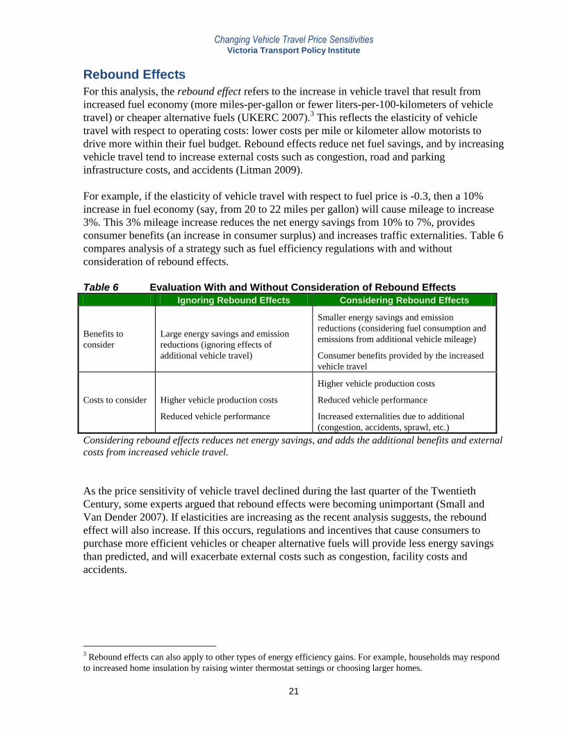
Rebound Effects
For this analysis, the rebound effect refers to the increase in vehicle travel that result from
increased fuel economy (more miles-per-gallon or fewer liters-per-100-kilometers of vehicle
travel) or cheaper alternative fuels (UKERC 2007).3 This reflects the elasticity of vehicle
travel with respect to operating costs: lower costs per mile or kilometer allow motorists to
drive more within their fuel budget. Rebound effects reduce net fuel savings, and by increasing
vehicle travel tend to increase external costs such as congestion, road and parking
infrastructure costs, and accidents (Litman 2009).
For example, if the elasticity of vehicle travel with respect to fuel price is -0.3, then a 10%
increase in fuel economy (say, from 20 to 22 miles per gallon) will cause mileage to increase
3%. This 3% mileage increase reduces the net energy savings from 10% to 7%, provides
consumer benefits (an increase in consumer surplus) and increases traffic externalities. Table 6
compares analysis of a strategy such as fuel efficiency regulations with and without
consideration of rebound effects.
Table 6 Evaluation With and Without Consideration of Rebound Effects
Ignoring Rebound Effects Considering Rebound Effects
Benefits to
consider
Large energy savings and emission
reductions (ignoring effects of
additional vehicle travel)
Smaller energy savings and emission
reductions (considering fuel consumption and
emissions from additional vehicle mileage)
Consumer benefits provided by the increased
vehicle travel
Costs to consider
Higher vehicle production costs
Reduced vehicle performance
Higher vehicle production costs
Reduced vehicle performance
Increased externalities due to additional
(congestion, accidents, sprawl, etc.)
Considering rebound effects reduces net energy savings, and adds the additional benefits and external
costs from increased vehicle travel.
As the price sensitivity of vehicle travel declined during the last quarter of the Twentieth
Century, some experts argued that rebound effects were becoming unimportant (Small and
Van Dender 2007). If elasticities are increasing as the recent analysis suggests, the rebound
effect will also increase. If this occurs, regulations and incentives that cause consumers to
purchase more efficient vehicles or cheaper alternative fuels will provide less energy savings
than predicted, and will exacerbate external costs such as congestion, facility costs and
accidents.
3 Rebound effects can also apply to other types of energy efficiency gains. For example, households may respond
to increased home insulation by raising winter thermostat settings or choosing larger homes.
Changing Vehicle Travel Price Sensitivities Victoria Transport Policy Institute
22
Policy Implications
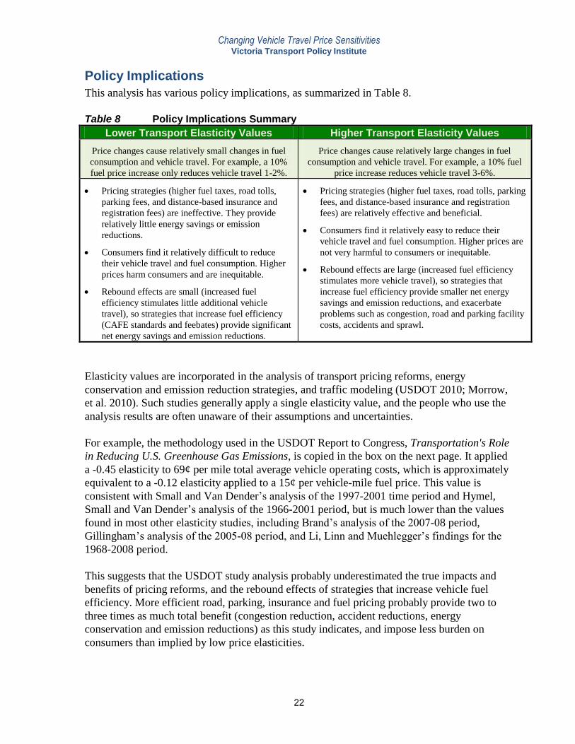
This analysis has various policy implications, as summarized in Table 8.
Table 8 Policy Implications Summary
Lower Transport Elasticity Values Higher Transport Elasticity Values
Price changes cause relatively small changes in fuel
consumption and vehicle travel. For example, a 10%
fuel price increase only reduces vehicle travel 1-2%.
Price changes cause relatively large changes in fuel
consumption and vehicle travel. For example, a 10% fuel
price increase reduces vehicle travel 3-6%.
Pricing strategies (higher fuel taxes, road tolls,
parking fees, and distance-based insurance and
registration fees) are ineffective. They provide
relatively little energy savings or emission
reductions.
Consumers find it relatively difficult to reduce
their vehicle travel and fuel consumption. Higher
prices harm consumers and are inequitable.
Rebound effects are small (increased fuel
efficiency stimulates little additional vehicle
travel), so strategies that increase fuel efficiency
(CAFE standards and feebates) provide significant
net energy savings and emission reductions.
Pricing strategies (higher fuel taxes, road tolls, parking
fees, and distance-based insurance and registration
fees) are relatively effective and beneficial.
Consumers find it relatively easy to reduce their
vehicle travel and fuel consumption. Higher prices are
not very harmful to consumers or inequitable.
Rebound effects are large (increased fuel efficiency
stimulates more vehicle travel), so strategies that
increase fuel efficiency provide smaller net energy
savings and emission reductions, and exacerbate
problems such as congestion, road and parking facility
costs, accidents and sprawl.
Elasticity values are incorporated in the analysis of transport pricing reforms, energy
conservation and emission reduction strategies, and traffic modeling (USDOT 2010; Morrow,
et al. 2010). Such studies generally apply a single elasticity value, and the people who use the
analysis results are often unaware of their assumptions and uncertainties.
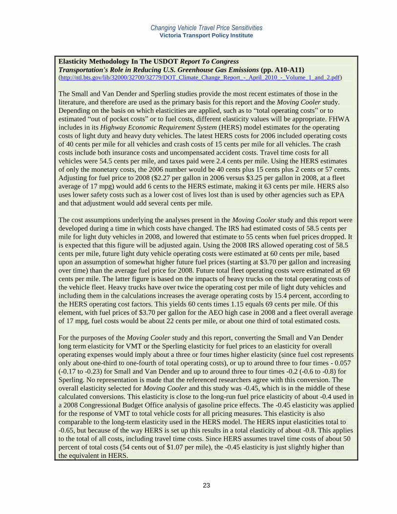
For example, the methodology used in the USDOT Report to Congress, Transportation's Role
in Reducing U.S. Greenhouse Gas Emissions, is copied in the box on the next page. It applied
a -0.45 elasticity to 69¢ per mile total average vehicle operating costs, which is approximately
equivalent to a -0.12 elasticity applied to a 15¢ per vehicle-mile fuel price. This value is
consistent with Small and Van Dender’s analysis of the 1997-2001 time period and Hymel,
Small and Van Dender’s analysis of the 1966-2001 period, but is much lower than the values
found in most other elasticity studies, including Brand’s analysis of the 2007-08 period,
Gillingham’s analysis of the 2005-08 period, and Li, Linn and Muehlegger’s findings for the
1968-2008 period.
This suggests that the USDOT study analysis probably underestimated the true impacts and
benefits of pricing reforms, and the rebound effects of strategies that increase vehicle fuel
efficiency. More efficient road, parking, insurance and fuel pricing probably provide two to
three times as much total benefit (congestion reduction, accident reductions, energy
conservation and emission reductions) as this study indicates, and impose less burden on
consumers than implied by low price elasticities.
Changing Vehicle Travel Price Sensitivities Victoria Transport Policy Institute
23
Elasticity Methodology In The USDOT Report To Congress
Transportation's Role in Reducing U.S. Greenhouse Gas Emissions (pp. A10-A11) (http://ntl.bts.gov/lib/32000/32700/32779/DOT_Climate_Change_Report_-_April_2010_-_Volume_1_and_2.pdf)
The Small and Van Dender and Sperling studies provide the most recent estimates of those in the
literature, and therefore are used as the primary basis for this report and the Moving Cooler study.
Depending on the basis on which elasticities are applied, such as to “total operating costs” or to
estimated “out of pocket costs” or to fuel costs, different elasticity values will be appropriate. FHWA
includes in its Highway Economic Requirement System (HERS) model estimates for the operating
costs of light duty and heavy duty vehicles. The latest HERS costs for 2006 included operating costs
of 40 cents per mile for all vehicles and crash costs of 15 cents per mile for all vehicles. The crash
costs include both insurance costs and uncompensated accident costs. Travel time costs for all
vehicles were 54.5 cents per mile, and taxes paid were 2.4 cents per mile. Using the HERS estimates
of only the monetary costs, the 2006 number would be 40 cents plus 15 cents plus 2 cents or 57 cents.
Adjusting for fuel price to 2008 ($2.27 per gallon in 2006 versus $3.25 per gallon in 2008, at a fleet
average of 17 mpg) would add 6 cents to the HERS estimate, making it 63 cents per mile. HERS also
uses lower safety costs such as a lower cost of lives lost than is used by other agencies such as EPA
and that adjustment would add several cents per mile.
The cost assumptions underlying the analyses present in the Moving Cooler study and this report were
developed during a time in which costs have changed. The IRS had estimated costs of 58.5 cents per
mile for light duty vehicles in 2008, and lowered that estimate to 55 cents when fuel prices dropped. It
is expected that this figure will be adjusted again. Using the 2008 IRS allowed operating cost of 58.5
cents per mile, future light duty vehicle operating costs were estimated at 60 cents per mile, based
upon an assumption of somewhat higher future fuel prices (starting at $3.70 per gallon and increasing
over time) than the average fuel price for 2008. Future total fleet operating costs were estimated at 69
cents per mile. The latter figure is based on the impacts of heavy trucks on the total operating costs of
the vehicle fleet. Heavy trucks have over twice the operating cost per mile of light duty vehicles and
including them in the calculations increases the average operating costs by 15.4 percent, according to
the HERS operating cost factors. This yields 60 cents times 1.15 equals 69 cents per mile. Of this
element, with fuel prices of $3.70 per gallon for the AEO high case in 2008 and a fleet overall average
of 17 mpg, fuel costs would be about 22 cents per mile, or about one third of total estimated costs.
For the purposes of the Moving Cooler study and this report, converting the Small and Van Dender
long term elasticity for VMT or the Sperling elasticity for fuel prices to an elasticity for overall
operating expenses would imply about a three or four times higher elasticity (since fuel cost represents
only about one-third to one-fourth of total operating costs), or up to around three to four times - 0.057
(-0.17 to -0.23) for Small and Van Dender and up to around three to four times -0.2 (-0.6 to -0.8) for
Sperling. No representation is made that the referenced researchers agree with this conversion. The
overall elasticity selected for Moving Cooler and this study was -0.45, which is in the middle of these
calculated conversions. This elasticity is close to the long-run fuel price elasticity of about -0.4 used in
a 2008 Congressional Budget Office analysis of gasoline price effects. The -0.45 elasticity was applied
for the response of VMT to total vehicle costs for all pricing measures. This elasticity is also
comparable to the long-term elasticity used in the HERS model. The HERS input elasticities total to
-0.65, but because of the way HERS is set up this results in a total elasticity of about -0.8. This applies
to the total of all costs, including travel time costs. Since HERS assumes travel time costs of about 50
percent of total costs (54 cents out of $1.07 per mile), the -0.45 elasticity is just slightly higher than
the equivalent in HERS.
Changing Vehicle Travel Price Sensitivities Victoria Transport Policy Institute
24
Research Recommendations
This report highlights the value of improving our understanding transportation price
sensitivities. Although numerous transport elasticity studies have been performed, many use
relatively simple models that account for a limited set of factors.
It would be useful for transportation professional organizations to sponsor meta-analyses of
transport elasticity studies to examine in detail the factors considered in previous studies and
recommends best practices for future studies, including standardized definitions, factors to
include in models, and analysis methodologies. Such research should identify how to best
incorporate various demographic, geographic and economic factors when evaluating price
effects, taking account insights from recent studies. For example, Li, Linn and Muehlegger
(2011) indicate that it is important to differentiate between price changes that consumers
consider temporary fluctuations with those that they consider durable. Other studies highlight
the importance of disaggregating effects by geographic location (Gillingham 2010).
This study identifies several factors that deserve consideration in future research:
Disaggregate the ways that consumers respond to higher fuel prices, including changes in
vehicle travel speed, vehicle mileage, fleet fuel economy, and location decisions.
Identify how various factors affect price sensitivities, including demographics (portion of
residents in different age and income classes), the magnitude of fuel prices relative to
household incomes, the magnitude and duration of price changes, geographic factors (how
price sensitivities vary between urban, suburban and rural areas), price method and frequency
(such as daily versus monthly parking fees), the quality of alternatives, the time period of
analysis, and the type of information and marketing provided to consumers (such as
information about transport options).
Investigate how sensitivities vary by pricing type and method, with special attention to the
transferability of fuel price elasticities to other types of transport pricing such as road, parking
and insurance. This should include, for example, analysis of the elasticity of vehicle
ownership in response to residential parking pricing.
Track how price sensitivities vary from one time period to another. In particular, investigate
the hypothesis that transport price sensitivities reached nadir in the last quarter of the
Twentieth Century and have since increased.
Apply sensitivity analysis to the evaluation of pricing reform impacts and benefits,
particularly higher elasticity values for studies that compare pricing reforms with other
congestion, energy conservation and emission reduction strategies.
Changing Vehicle Travel Price Sensitivities Victoria Transport Policy Institute
25
Conclusions
There is growing interest in transportation pricing reforms to help achieve various planning
objectives such as congestion reduction, facility cost savings, traffic safety, energy
conservation and emission reductions. Their impacts and benefits are affected by the price
elasticities of fuel and vehicle travel. Low elasticities imply that such reforms are relatively
ineffective at achieving objectives, that price increases significantly harm consumers, and that
alternative strategies that increase vehicle fuel efficiency have minimal rebound effects.
Conversely, high elasticities imply that pricing reforms are effective and beneficial, harm
consumers relatively little, and strategies that increase vehicle fuel economy have significant
rebound effects that reduce energy savings and increase external costs such as congestion,
facility costs and accidents.
Most studies indicate long-run fuel price elasticities to be -0.4 to -0.8, and long-run elasticities
of vehicle travel with respect to fuel price to be -0.2 to -0.3. Significantly lower elasticities
(under -0.2 for fuel and -0.1 for vehicle travel) were found in the U.S. between 1970 and 2004,
which probably reflected demographic and economic trends during that period including rising
employment rates and real incomes, declining real fuel prices, highway expansions and
suburbanization. Many of these trends are now reversing. As a result, elasticities are likely to
increase to more normal levels.
Recent research provides insights useful for evaluating pricing reforms. Elasticities tend to
increase over time as consumers incorporate price changes in more long-term decisions such
as vehicle purchases and home locations. Elasticities tend to increase if consumers have better
accessibility options. Elasticities are higher for price increases consumers consider durable,
such as tax increases, than price increases that consumers consider temporary such as
occasional oil price spikes.
Relatively low elasticity values have been incorporated into various policy analyses, which
likely underestimated price reform effectiveness and benefits, and exaggerated the
effectiveness higher vehicle fuel efficiency regulations and incentives. If price elasticities are
returning to more normal levels, these reforms actually provide far greater benefit (congestion
and accident reductions, energy conservation and emission reductions) than analyses indicate.
This issue deserves more research. Evidence of rising price elasticities is still preliminary. It is
therefore important that policy analysts, modelers, and decision-makers understand these
issues and trends. Analysts should apply sensitivity analysis, including relatively high
elasticity values when evaluating transport policies.
Changing Vehicle Travel Price Sensitivities Victoria Transport Policy Institute
26
References
J. Agras and D. Chapman (1999), “The Kyoto Protocol, CAFE Standards, and Gasoline Taxes,”
Contemporary Economic Policy, Vol. 17 No. 3; http://onlinelibrary.wiley.com/doi/10.1111/j.1465-
7287.1999.tb00683.x/abstract.
BLS (2007 and 2008), Consumer Expenditure Survey, Bureau of Labor Statistics (www.bls.gov); at
www.bls.gov/cex/home.htm.
François Boilard (2010), “Gasoline Demand In Canada: Parameter Stability Analysis,” EnerInfo, Vol.
15/3, Fall, Centre for Data and Analysis in Transportation, Université Laval (www.cdat.ecn.ulaval.ca);
at www.fss.ulaval.ca/cms_recherche/upload/cdat_en/fichiers/ioiriofo,_vo.15,_oumbir_3,_f_2010.pdf.
Dan Brand (2009), Impacts of Higher Fuel Costs, Federal Highway Administration,
(www.fhwa.dot.gov); at www.fhwa.dot.gov/policy/otps/innovation/issue1/impacts.htm.
BTS (2001), National Transportation Statistics, Bureau of Transportation Statistics (www.bts.gov); at
www.vtpi.org/fueltrends.xls.
CBO (2005), Limiting Carbon Dioxide Emissions: Prices Versus Caps, Congressional Budget Office
(www.cbo.gov); at www.cbo.gov/ftpdoc.cfm?index=6148&type=0.
CBO (2008), Effects of Gasoline Prices on Driving Behavior and Vehicle Markets, Congressional
Budget Office (www.cbo.gov); at www.cbo.gov/ftpdocs/88xx/doc8893/01-14-GasolinePrices.pdf.
CERA (2006), Gasoline and the American People, Cambridge Energy Research Associates
(www2.cera.com/gasoline); at www2.cera.com/gasoline/summary.
Molly Espey (1996), “Explaining The Variation In Elasticity Estimates Of Gasoline Demand In The
United States: A Meta-Analysis,” Energy Journal, Vol. 17, No. 3, pp. 49-60; at
http://zonecours.hec.ca/documents/H2008-1-1529402.gasolinedemand.pdf.
EIA (2010), Annual Energy Outlook, U.S. Energy Information Administration (www.eia.gov); at
www.eia.gov/forecasts/aeo.
Kenneth Gillingham (2010), Identifying the Elasticity of Driving: Evidence from a Gasoline Price
Shock in California, Stanford University (www.stanford.edu); at
www.stanford.edu/~kgilling/Gillingham_IdentifyingElasticityofDriving.pdf.
GIZ (2011/2012), International Fuel Prices, German Agency for Technical Cooperation
(www.gtz.de/en/themen/29957.htm).
Stephen Glaister and Dan Graham (2002), “The Demand for Automobile Fuel: A Survey of
Elasticities,” Journal of Transport Economics and Policy, Vol. 36, No. 1, pp. 1-25; at
www.ingentaconnect.com/content/lse/jtep/2002/00000036/00000001/art00001.
Phil Goodwin, Joyce Dargay and Mark Hanly (2004), “Elasticities of Road Traffic and Fuel Consumption
With Respect to Price and Income: A Review,” Transport Reviews (www.tandf.co.uk), Vol. 24/3, May, pp.
275-292.
Changing Vehicle Travel Price Sensitivities Victoria Transport Policy Institute
27
Zhan Guo, et al. (2011), The Intersection of Urban Form and Mileage Fees: Findings from the
Oregon Road User Fee Pilot Program, Report 10-04, Mineta Transportation Institute
(http://transweb.sjsu.edu); at http://transweb.sjsu.edu/PDFs/research/2909_10-04.pdf.
Zachary Howard and Clark Williams-Derry (2012), How Much Do Drivers Pay For A Quicker
Commute? New Evidence Suggests That It's Less Than We Think, Sightline Institute (www.sightline.org);
at (http://daily.sightline.org/2012/08/01/how-much-do-drivers-pay-for-a-quicker-commute.
Jonathan E. Hughes, Christopher R. Knittel and Daniel Sperling (2006), Evidence of a Shift in the
Short-Run Price Elasticity of Gasoline Demand, Working Paper No. 12530, National Bureau of
Economic Research (www.nber.org); at http://papers.nber.org/papers/W12530.
Kent M. Hymel, Kenneth A. Small and Kurt Van Dender (2010), “Induced Demand And Rebound
Effects In Road Transport,” Transportation Research B (www.elsevier.com/locate/trb), Vol. 44, Issue
10, December, pp. 1220-1241; at www.socsci.uci.edu/~ksmall/Rebound_congestion_27.pdf.
INRIX (2008), The Impact of Fuel Prices on Consumer Behavior and Traffic Congestion, INRIX
(www.inrix.com); at http://scorecard.inrix.com/scorecard.
Olof Johansson and Lee Schipper (1997), “Measuring the Long-Run Fuel Demand for Cars,” Journal
of Transport Economics and Policy, Vol. 31, No. 3, pp. 277-292.
Charles Komanoff (2008), Gasoline Price-Elasticity Spreadsheet, Komanoff Energy Consulting
(www.komanoff.net/oil_9_11/Gasoline_Price_Elasticity.xls).
Jaimin Lee, Sangyong Han and Chang-Woon Lee (2009), Oil Price and Travel Demand, Korea
Transport Institute (http://english.koti.re.kr).
Shanjun Li, Joshua Linn and Erich Muehlegger (2011), Gasoline Taxes and Consumer Behavior,
Stanford (http://economics.stanford.edu); at http://economics.stanford.edu/files/muehlegger3_15.pdf.
Gar W. Lipow (2008), Price-Elasticity of Energy Demand: A Bibliography, Carbon Tax Center
(www.carbontax.org); at www.carbontax.org/wp-content/uploads/2007/10/elasticity_biblio_lipow.doc.
Todd Litman (2001), “Generated Traffic: Implications for Transport Planning,” ITE Journal, Vol. 71,
No. 4, Institute of Transportation Engineers (www.ite.org), April, pp. 38-47; at
www.vtpi.org/gentraf.pdf.
Todd Litman (2005), “Efficient Vehicles Versus Efficient Transportation: Comparing Transportation Energy
Conservation Strategies,” Transport Policy, Vol. 12/2, March, pp. 121-129; at www.vtpi.org/cafe.pdf.
Todd Litman (2006), The Future Isn’t What It Used To Be: Changing Trends And Their Implications
For Transport Planning, Victoria Transport Policy Institute (www.vtpi.org); at
www.vtpi.org/future.pdf; originally published as “Changing Travel Demand: Implications for
Transport Planning,” ITE Journal, Vol. 76, No. 9, (www.ite.org), September, pp. 27-33.
Todd Litman (2009), Transportation Cost and Benefit Analysis, VTPI (www.vtpi.org/tca).
Todd Litman (2011), Transportation Elasticities: How Prices and Other Factors Affect Travel
Behavior, Victoria Transport Policy Institute (www.vtpi.org); at www.vtpi.org/elasticities.pdf.
Changing Vehicle Travel Price Sensitivities Victoria Transport Policy Institute
28
Todd Litman (2012), “Changing North American Vehicle-Travel Price Sensitivities: Implications For
Transport and Energy Policy,” Transport Policy, http://dx.doi.org/10.1016/j.tranpol.2012.06.010.
Nicholas P. Lutsey and Daniel Sperling (2005), “Energy Efficiency, Fuel Economy, and Policy
Implications,” Transportation Research Record 1941, TRB (www.trb.org), pp. 8 - 17.
McKinsey (2007), Reducing U.S. Greenhouse Gas Emissions - How Much at What Cost - US
Greenhouse Gas Abatement Mapping Project, McKinsey & Company (www.mckinsey.com); at
www.mckinsey.com/clientservice/ccsi/pdf/US_ghg_final_report.pdf.
Raven Molloy and Hui Shan (2011), The Effect of Gasoline Prices on Household Location, Federal Reserve
Board (https://federalreserve.gov); at https://federalreserve.gov/pubs/feds/2010/201036/201036pap.pdf.
W. Ross Morrow, Kelly Sims Gallagher, Gustavo Collantes and Henry Lee (2010), Analysis of Policies
to Reduce Oil Consumption and Greenhouse-Gas Emissions from the U.S. Transportation Sector,
Kennedy School of Government, Harvard University (http://belfercenter.ksg.harvard.edu); at http://belfercenter.ksg.harvard.edu/files/Policies%20to%20Reduce%20Oil%20Consumption%20and%20Greenhouse
%20Gas%20Emissions%20from%20Transportation.pdf.
NCHRP (2006), Estimating Toll Road Demand and Revenue, NCHRP Synthesis 364, TRB
(www.trb.org); at: http://onlinepubs.trb.org/onlinepubs/nchrp/nchrp_syn_364.pdf.
OECD (2005), OECD in Figures, ISBN 9264013059, Organization for Economic Cooperation and
Development (www.oecd.org/infigures); in www.vtpi.org/OECD2006.xls.
Tae Hoon Oum, W.G. Waters II, and Jong-Say Yong (1992), “Concepts of Price Elasticities of
Transport Demand and Recent Empirical Estimates, Journal of Transport Economics, May, pp. 139-
154; based on A Survey of Recent Estimates of Price Elasticities of Travel Demand, (1990) World
Bank (www.worldbank.org).
Fred Pearce (2011), “End of the Road for Motormania,” New Scientist, 2825 (www.newscientist.com);
at www.newscientist.com/article/mg21128255.600-the-end-of-the-road-for-motormania.html.
PSRC (2005), Traffic Choices Study, Puget Sound Regional Council (http://psrc.org); at
http://psrc.org/assets/37/summaryreport.pdf.
Robert Puentes (2008), The Road…Less Traveled: An Analysis of Vehicle Miles Traveled Trends in
the U.S., Brooking Institution (www.brookings.edu); at
www.brookings.edu/reports/2008/1216_transportation_tomer_puentes.aspx.
SACOG (2008), Impact of Gas Prices on Travel Behavior, Sacramento Area Council of Governments
(www.sacog.org); at
www.sacog.org/rucs/wiki/index.php/Impact_of_Gas_Prices_on_Travel_Behavior.
Paul Schimek (1997), “Gasoline and Travel Demand Models Using Time Series and Cross-Section Data
from the United States,” Transportation Research Record 1558, TRB (www.trb.org), pp. 83-89.
Changing Vehicle Travel Price Sensitivities Victoria Transport Policy Institute
29
Kenneth Small and Kurt Van Dender (2005), The Effect of Improved Fuel Economy on Vehicle Miles
Traveled: Estimating the Rebound Effect Using U.S. State Data, 1966-2001, University of California
Energy Institute's (UCEI) (www.ucei.berkeley.edu); at www.ucei.berkeley.edu/PDF/EPE_014.pdf.
Kenneth A. Small and Kurt Van Dender (2007), “Fuel Efficiency and Motor Vehicle Travel: The
Declining Rebound Effect,” Energy Journal, Vol. 28, No. 1, pp. 25-51; at
www.econ.uci.edu/docs/2005-06/Small-03.pdf.
Elisheba Spiller and Heather M. Stephens (2012), The Heterogeneous Effects of Gasoline Taxes: Why
Where We Live Matters, Resources for the Future (www.rff.org); at
www.rff.org/RFF/Documents/RFF-DP-12-30.pdf; complete report at
http://papers.ssrn.com/sol3/papers.cfm?abstract_id=2129396.
Thomas Sterner (2006), “Fuel Taxes: An Important Instrument for Climate Policy,” Energy Policy, Vol.
35. pp. 3194–3202; at www.hgu.gu.se/files/nationalekonomi/personal/thomas%20sterner/a78.pdf.
TRB (2009), Strategies for Reducing the Impacts of Surface Transportation on Global Climate
Change, NCHRP 20-24, TRB (www.trb.org); www.trb.org/trbnet/ProjectDisplay.asp?ProjectID=2113.
VTPI (2010), Online TDM Encyclopedia, Victoria Transport Policy Institute (www.vtpi.org/tca).
VTPI (2011), U.S. Fuel Trends Spreadsheet, Victoria Transport Policy Institute
(www.vtpi.org/fueltrends.xls).
UKERC (2007), The Rebound Effect: An Assessment Of The Evidence For Economy-Wide Energy
Savings From Improved Energy Efficiency, UK Energy Research Centre (www.ukerc.ac.uk); at
www.ukerc.ac.uk/support/tiki-index.php?page=ReboundEffect.
US Census (2010a), CPS Population and Per Capita Money Income, All Races: 1967 to 2010, Table
P-1, U.S. Census Bureau (www.census.gov); at
www.census.gov/hhes/www/income/data/historical/people/2010/P01AR_2010.xls.
US Census (2010a), Work Experience--All Workers by Median Earnings and Sex: 1967 to 2010,
Table P-41, U.S. Census Bureau (www.census.gov); at
www.census.gov/hhes/www/income/data/historical/people/2010/P01AR_2010.xls.
USDOT (2010), Transportation's Role in Reducing U.S. Greenhouse Gas Emissions: Volume 1,
Report to Congress, U.S. Department of Transportation (www.dot.gov), at
http://ntl.bts.gov/lib/32000/32700/32779/DOT_Climate_Change_Report_-_April_2010_-
_Volume_1_and_2.pdf.
Clark Williams-Derry (2010), “Dude, Where Are My Cars?” Sightline Institute (www.sightline.org) at
http://daily.sightline.org/daily_score/series/dude-where-are-my-cars.
Clark Williams-Derry (2011), Toll Avoidance And Transportation Funding: Official Estimates
Frequently Overestimate Traffic And Revenue For Toll Roads, Sightline Institute (www.sightline.org);
at www.sightline.org/research/sprawl/toll-avoidance-and-transportation-funding.
www.vtpi.org/VMT_Elasticities.pdf