chalmers publication...

Chalmers Publication Library

Robust adaptive beamforming for MIMO monopulse radar

This document has been downloaded from Chalmers Publication Library (CPL). It is the author´s

version of a work that was accepted for publication in:

Proceedings of SPIE - The International Society for Optical Engineering (ISSN: 0277786X)

Citation for the published paper:Rowe, W. ; Ström, M. ; Li, J. (2013) "Robust adaptive beamforming for MIMO monopulseradar". Proceedings of SPIE - The International Society for Optical Engineering, vol. 8714

http://dx.doi.org/10.1117/12.2015805

Downloaded from: http://publications.lib.chalmers.se/publication/186987

Notice: Changes introduced as a result of publishing processes such as copy-editing and

formatting may not be reflected in this document. For a definitive version of this work, please refer

to the published source. Please note that access to the published version might require a

subscription.

Chalmers Publication Library (CPL) offers the possibility of retrieving research publications produced at ChalmersUniversity of Technology. It covers all types of publications: articles, dissertations, licentiate theses, masters theses,conference papers, reports etc. Since 2006 it is the official tool for Chalmers official publication statistics. To ensure thatChalmers research results are disseminated as widely as possible, an Open Access Policy has been adopted.The CPL service is administrated and maintained by Chalmers Library.

(article starts on next page)

http://dx.doi.org/10.1117/12.2015805

http://publications.lib.chalmers.se/publication/186987

Robust adaptive beamforming for MIMO monopulse radar

William Rowe, Marie Strom, Jian Li and Petre Stoica ∗

ABSTRACT

Researchers have recently proposed a widely separated multiple-input multiple-output (MIMO) radar usingmonopulse angle estimation techniques for target tracking. The widely separated antennas provide improvedtracking performance by mitigating complex target radar cross-section fades and angle scintillation. An adaptivearray is necessary in this paradigm because the direct path from any transmitter could act as a jammer ata receiver. When the target-free covariance matrix is not available, it is critical to include robustness intothe adaptive beamformer weights. This work explores methods of robust adaptive monopulse beamformingtechniques for MIMO tracking radar.

1. INTRODUCTION

Widely separated multiple-input multiple-output (MIMO) radar systems are of significant interest for trackingapplications because of their ability to mitigate angular glint. The majority of real world targets act as complexscatters rather than ideal scatters which introduces the so-called target noise into the problem.1,2 This noisecan manifest itself as amplitude and angle scintillations. The angle scintillations, commonly referred to as glint,is of great concern in tracking radar because it can cause the angle estimate to move well beyond the actualtrue target angle.3 The typical monopulse angle estimation techniques (or sequential lobing techniques) cannotaccount for glint due to the physical nature of the phenomenon which can be viewed as phase-front distortion.4,5

The best technique for accounting for glint has long been known to be to mitigate the physical phenomenonin the illumination scheme.4,6 The two methods of glint mitigation proposed have been frequency diversity andangle diversity since target glint has been shown to have a strong negative correlation with radar cross-section(RCS) nulls or fades. Since RCS is a function of carrier wavelength and aspect angle, diversity in either domainshould lower the risk that the current RCS is near a null. This is one of the major motivations for utilizing awidely separated MIMO scheme.7

Widely separated MIMO radar has been extended to the tracking radar problem utilizing monopulse angleestimation techniques.8 In addition to any external interference such as jamming, for widely separated MIMOtracking radars any line of sight paths between transmitter and receiver may act as interference (via antennapattern sidelobes) as well. This problem produces the need to introduce either temporal or spatial filtering.Temporal filtering (or blanking) may overlap with the expected target delay of a specific transmitter/receiverpair. The transmitter may also place nulls in the angles corresponding to the receivers which would requireadaptive transmit beamforming. Similarly, the receiver may place nulls in the direction of the transmitters.Since it is more likely that the receiver will be performing adaptive array processing already to combat jamming,we consider the latter solution in this paper.

The adaptive array angle estimation problem for monopulse has been studied in the past for single-inputsingle-output and phased array radars.9 The optimal beamforming weights have been derived for arbitrary arraylayouts and subarray configurations.10 The majority of these exisiting methods utilize maximum likelihoodestimates where the noise is assumed to be complex Gaussian with zero mean and static covariance matrix.9,10

Unfortunately, the environment noise may not follow a Gaussian distribution. These methods also utilize thetarget free covariance matrix which may not be obtainable in all scenarios.

∗This work was supported in part by the SMART fellowship program and the University of Florida Research Foundation (UFRF)Professorships Award. William Rowe, and Jian Li are with the department of Electrical and Computer Engineering, University ofFlorida, Gainesville, Florida 32611, [email protected], [email protected]. Jian Li is also affiliated with the IAA, Inc. Gainesville,Florida 32611. Marie Strom is with Chalmers University of Technology, Department of Signals and Systems, 412 96 Goteborg,Sweden and Saab EDS, Solhusgatan 10, Kallebacks Teknikpark, 412 89 Goteborg, Sweden, [email protected] Petre Stoicais with the department of Information Technology, Division of Systems and Control, Uppsala University, 751 05 Uppsala, Sweden,[email protected].

In the original MIMO Monopulse tracking system proposed, an amplitude monopulse system that used theCapon beamformer was described.8 This approach may suffer in performance because the monopulse estimateutilizes symmetry between the squinted beams to generate a linear monopulse ratio. There is no guarantee thatthe Capon beams will provide such symmetry when interference is close to the mainbeam or number of snapshotsavailable to estimate the target free covariance matrix is low.

In this work we examine three different beamforming approaches for adaptive amplitude monopulse. In theseapproaches we consider a joint design of the left and right beams for amplitude monopulse. The first method,called linearly constrained Capon (LCC), resolves the problem of a lack of symmetry when using the Caponbeamformer, but it requires the target free covariance matrix. The second method introduces a norm constraintinto the LCC problem. We call this method norm and linearly constrained Capon Beamformer (NLCC) and itcan directly utilize the target return samples to estimate the covariance matrix. The final method, which is anextension of the adaptive matrix approach (AMA), allows for the suppression of direct path interference betweentransmitters and receivers by utilizing the knowledge of the scene geometry.

In the next section a brief review of monopulse estimation fundamentals will be presented to motivate thebeamforming problem. This will be followed by the fundamentals of the joint beam design problem for MIMOmonopulse tracking. By using these fundamentals, the LCC, NLCC, and AMA approaches will be presented.The performance will be evaluated by numerical simulations in the fourth section. Finally, we will summarizeour results and conclude this paper.

We will briefly describe notation that will be used in this paper. A column vector is denoted by a boldfacelower case letter a and a matrix is denoted by an boldface upper case A. The target free covariance matrix willbe denoted as Q and the covariance matrix containing the target will be denoted by R. We also denote (·)H asthe Hermetian transpose of a vector or matrix. The operator Tr(·) denotes a matrix trace operation. Finally wedenote ⊗ as a Kronecker matrix product.

2. MONOPULSE FUNDAMENTALS

Monopulse is a computationally efficient method of measuring a target’s angular error that is based on a firstorder Taylor expansion approximation. The concept is to generate an error signal relative to the expected targetposition.11 This can be achieved by either using multiple phase centers (phase monopulse) or by using squintedbeams (amplitude monopulse). A difference (∆) and a sum (Σ) channel is formed from the multiple beams. Theratio ∆/Σ is called the monopulse ratio. When the beamshapes are symmetric, then the ratio is linear withrespect to the true target angle in a local region. Using the Taylor expansion of the monopulse ratio, we havethe following expression for estimating the target angle for uniform linear arrays (ULA):

sin(θ) = sin(θo)− γ−1 ∆

Σ. (1)

Here θo is our original target angle estimate, θ is the estimated target angle, and γ is the slope of the monopulseratio.10 If the monopulse ratio is not approximated by a linear function, then the angle estimate will degrade.The performance of the monopulse estimate is dependent on noise, clutter, and jammer power in the receivedsignal as well. For this reason all monopulse beams should be designed to posses low sidelobe levels and/orjammer rejection.11

For amplitude monopulse two beams are squinted from the estimated target angle θo at angles θL and θR.The beams are squinted off by approximately half the angular resolution determined by the array size. Forthe data-independent amplitude monopulse, we assume that two beams wL and wR are formed using Taylorwindowed standard beamforming vectors. The difference and sum channels are then defined as:

∆ = |wHR y| − |wH

L y| (2)

Σ = |wHR y|+ |wH

L y|,

where y is the received data vector.

This data-independent method is computationally efficient, easy to implement and provides good performancein most scenarios. However, the data-independent approach is not robust against jammers and interference. Inthe widely separated MIMO scenario, the direct path between a transmitter and receiver pair could createunwanted interference even when it is arriving in the sidelobe region. We will propose adaptive amplitudebeamforming methods for these MIMO systems.

3. ADAPTIVE AMPLITUDE MONOPULSE

An adaptive approach to the monopulse estimate was developed in 1976 for single-input single-output systems,9

and an excellent overview containing the modern theory for adaptive monopulse estimation was presented in2006.10 In both these solutions, the ideal adaptive monopulse estimate is a phase monopulse type estimate.The estimate is based on the assumption that the noise and interference distribution is complex normal withcovariance matrix Q. The dependence on the target free covariance matrix Q can pose a practical problem inreal world systems when target free samples are limited or not available.

Even if Q is available when utilizing the Capon beamformer, as proposed in the original MIMO monopulsepaper,8 to generate amplitude monopulse there is no guarantee that the beams will produce a linear monopulseratio. A loss of linearity degrades the angle estimate approximation in (1). Suppose that the linearity was nota problem, the Capon beamformer still requires Q. The reason the Capon beamformer must use Q instead oftarget sample covariance matrix R is because amplitude monopulse attempts to squint two beams from θo withthe assumption that our target lies between the two beam focal points. Since R contains the target arrivingwith angle between the two squinted beam peaks, the Capon beamformer will regard it as interference andtry to null the target return. This can be resolved by defocusing the Capon beamformer using robust Caponbeamforming (RCB) techniques.12 In the widely separated MIMO radar scenario, it would be logical to forcenulls into the antenna beampattern in angles corresponding to direct paths between transmitter and receiverpairs. The adaptive matrix approach (AMA) allows for the design of beampatterns that can place desired nullswhile maintaining adaptive capabilities.13

In this section we propose three methods to develop an adaptive amplitude monopulse estimate. The firstmethod, called linearaly constrained Capon (LCC) amplitude monopulse, extends the Capon beamformer withthe introduction of more linear constraints when a target free covariance matrix estimate is available. Thismethod maintains a more linear monopulse ratio compared to the standard Capon method. The second method,called norm and linearly constrained Capon (NLCC) amplitude monopulse, extends the norm constraint RCB toinclude more linear constraints to help preserve the monopulse ratio. We also present a method of calculating thediagonal loading level for a given norm constraint. Finally, we present a method using the AMA for amplitudemonopulse for scenarios where unwanted angles are known a priori.

3.1 Joint Beam Design Basics

We begin our discussion by laying out the model and a basic joint beamshape design metric. We assume thatour array has a known (via calibration) steering vector a(θ) ∈ CN×1, where N is the number of elements in ourarray and θ ∈ (−90◦, 90◦]. We also assume that the array has been critically sampled. For amplitude monopulsewe wish to jointly design two adaptive beams at angles θL and θR. If we utilized a standard Capon beamformingcost function we would get:

minimizewL,wR

wHL QwL + wH

R QwR

subject to wHL a(θL) = wH

R a(θR) = 1.(3)

This problem can be rewritten into the standard Capon Beamforming problem by manipulating the vectorsand matrices. Let w = [wH

L wHR ]H , b = [1 1], and Q = I2×2 ⊗Q. We then create a linear constraint matrix A

such that:

A =

[a(θL) 0N×10N×1 a(θR)

].

Using w, Q,b, andA, we reformulate the joint beamforming problem as

minimizew

wHQw

subject to wHA = b.(4)

This is a well known problem.14 A closed form solution to it is given by

w = (Q−1A)(AHQ−1A)−1bH . (5)

Here the first N elements of w correspond to wL and the last N elements correspond to wR. This problemwould result in the standard Capon beams since the linear constraints on the beams are the same. Next we willshow that the inclusion of more linear constraints into the matrix A and vector b will allow for the joint designof adaptive beams that maintain good monopulse performance.

3.2 Adaptive Amplitude Monopulse Beamforming

When the target free covariance matrix is available the optimal beamforming vector is given by the Caponestimator. This does not imply that the monopulse ratio formed by two squinted Capon estimators will form agood monopulse ratio. It is easy to show through numerical examples that an amplitude monopulse ratio formedwith Capon beams will have non-ideal properties such as lack of linearity and non-zero response at zero angularerror.

We propose to rectify such problems by the inclusion of three more linear constraints into the problem posedin (4). The first additional constraint is to force equality between the beams at the expected target position.This removes the non-zero monopulse ratio response at zero error. The next two additional constraints helppromote linearity by promoting a decreasing beam slope in the measurement region. The modified problem is

minimizewL,wR

wHL QwL + wH

R QwR

subject to wHL a(θL) = wH

R a(θR) = 1

wHL a(θo)−wH

R a(θo) = 0

wHL a(θR) = wH

R a(θL) = α,

(6)

where α is a user parameter. Our empirical findings showed that α =√.1 adequately promoted a linear

monopulse ratio.

Using the same approach in converting (3) to (4), we will rewrite (6) as:

minimizew

wHQw

subject to wHA = b,(7)

where w and Q are defined as in (4). We let

A =

[a(θL) 0N×1 a(θo) a(θR) 0N×10N×1 a(θR) −a(θo) 0N×1 a(θL)

]and

b =[1 1 0 α α

].

The solution is given in (5).

This approach overcomes the problems with using just the standard Capon beamformer for amplitudemonopulse estimation by providing a zero monopulse ratio at zero error and having a linear monopulse ra-tio. The method only works though when Q is available. When it is not available, the method’s performancewill degrade.

3.3 Robust Adaptive Amplitude Monopulse Beamforming

Researchers have considered robust Capon beamforming techniques and presented several different methods. Aubiquitous theme around all of the methods is diagonal loading. The diagonal loading coefficient effectivelydefocuses the Capon beamformer allowing for uncertainty in target angle or array calibration.12 The monopulseproblem assumes that the target angle is not known perfectly, but it should be near the expected angle θo. Thisassumption naturally poses a scenario for RCB when only the covariance matrix R is available.

We now propose an RCB method to provide the beamforming weights for adaptive amplitude monopulse.We utilize the same constraints as posed in (7) plus we include a norm constraint on our beamforming vector. Inthis method we assume that Q is not available and R must be estimated instead. First we denote R = I2×2⊗Rand then write the joint beamforming problem as

minimizew

wHRw

subject to wHA = b

‖ w ‖ ≤ ζ.

(8)

We attempt to solve (8) using Lagrange multipliers. This results in the following minimization-maximizationproblem

maxµ,λ

minw

wHRw − (wHA− b)µ− µH(AHw − bH) + λ(wHw − ζ)

subject to λ ≥ 0,(9)

where µ ∈ CL×1 and L is the number of columns of A. Let g1(w,µ, λ) = wHRw− (wHA−b)µ−µH(AHw−bH) + λ(wHw − ζ), and by completing the square the cost function can be written as

g1(w,µ, λ) = (w− (R + λI)−1Aµ)H(R + λI)(w− (R + λI)−1Aµ)−µHAH(R + λI)−1Aµ+ bµ+µHbH − λζ.

The minimizing w given µ, λ then iswopt = (R + λI)−1Aµ. (10)

Then we denote g2(µ, λ) = g1(wopt,µ, λ) where

g2(µ, λ) = −µHAH(R + λI)−1Aµ + bµ + µHbH − λζ.

The optimal µ given λ can then be found by calculating the derivative of g2(µ, λ) with respect to µ,

∂g2(µ, λ)

∂µ= −2AH(R + λI)−1Aµ + 2bH = 0.

Solving for µ results inµopt = (AH(R + λI)−1A)−1bH .

Then denoting g3(λ) = g2(µopt, λ) gives

g3(λ) = b(AH(R + λI)−1A)−1bH − λζ. (11)

The function g3(λ) will be utilized in the calculation of the diagonal loading coefficient λ. Before consideringthe problem of finding λ, note that we have derived the solution for a norm constrained robust beamformer withadditional linear constraints as a function of λ. Specifically that

wopt(λ) = (R + λI)−1A(AH(R + λI)−1A)−1bH (12)

which is just the diagonally loaded solution from the previous section. When λ = 0 the wopt is similar to

the LCC solution in (5). If λ is much larger than the largest eigenvalue of R (which we denote σmax), then

wopt ≈ A(AHA)−1bH which is similar to the beamformer solution. This observation gives an approximatebound on λ of 0 ≤ λ ≤ 10σmax.

To find λ we utilize the eigenvalue decomposition of R to simplify the required matrix inversions and toestimate bounds for λ. This is a one time expensive computation compared to the repeated inversions of R thatwould be required otherwise. Let R = UΓUH be the eigenvalue decomposition of R and let Z = UHA. Usingthe eigenvalue decomposition in (11) results in

g3(λ) = b(AH(UΓUH + λI)−1A)−1bH − λζ= b(ZH(Γ + λI)−1Z)−1bH − λζ.

To find the optimal parameter λ, we first calculate the partial derivative of g3(λ)

∂g3(λ)

∂λ= b(ZH(Γ + λI)−1Z)−1ZH(Γ + λI)−2Z(ZH(Γ + λI)−1Z)−1bH − ζ. (13)

This function can be shown to be monotonically decreasing when λ ≥ 0 and Γ is positive semi-definite (seeAppendix). We define the function h(λ) as

h(λ) = b(ZH(Γ + λI)−1Z)−1ZH(Γ + λI)−2Z(ZH(Γ + λI)−1Z)−1bH . (14)

Combining the fact that h(λ) is monotonically decreasing and the bounds for λ implies that ζmax = h(0) andζmin = h(10σmax). If ζ ≤ ζmin or ζ ≥ ζmax, then there is no optimal λ for that ζ. Given that ζ is in bounds, ifh(10σmax) > ζ then λopt = 10σmax using our limit on λ. Otherwise, we can calculate the optimal λ by findingthe zero crossing of h(λ)− ζ using a root finding algorithm such as a bisection method or Newton’s method.

Table 1: Norm and Linearly Constrained Capon Beamforming for Amplitude Monopulse

Step 0 - Initialize: Calculate the eignevalue decom-position: R = UΓUH and Z = UHAStep 1: Check h(10σmax) ≤ ζ ≤ h(0)Step 2: If h(10σmax) > ζ then λ = 10σmax.Step 3: Else λ is the value that satisfies h(λ)− ζ = 0.Step 4: w = U(Γ + λI)−1Z(ZH(Γ + λI)−1Z)−1bH

When λ is calculated then w can be calculated as shown in (12). However, a more computationally efficientmethod is using the eigenvalue decomposition as shown in Table 1. The procedure is effective when the targetfree covariance matrix is not available. In our simulations, ζ = 2.5 was found to be an effective norm-constraintthat still preserved a linear monopulse ratio.

3.4 Adaptive Matrix Approach Amplitude Monopulse Beamforming

For a MIMO radar, direct paths between the transmitting antennas and the receiver can be regarded as interferingsignals. If we have knowledge about the locations of the transmitters, then the direct paths could be cancelledout by designing beampatterns with nulls in these locations. Such a beampattern can be achieved by optimizinga weight matrix for the antenna array output, and an algorithm to do this adaptively is the AMA.13 With thismethod, which does not require knowledge of the target free covariance matrix, we can find a weight matrixwhich imposes nulls in the directions of the transmitters, as well as constraints on the sidelobe level.

For the AMA we introduce the weight matrices WR and WL associated with the right and left beam,respectively, and let TR = WRWH

R and TL = WLWHL . Our objective is to find TR and TL which yield low

sidelobe levels while maintaining the desired power and cancelling the effect of the transmitters. Following the

methodology laid out in the original work,13 the AMA can be formulated as

minimizeTR,TL

Tr(R(TR + TL))

subject to a(θR)HTRa(θR) = a(θL)HTLa(θL) = 1

a(θo)H(TR −TL)a(θo) = 0

a(θL)HTRa(θL) ≤ αa(θR)HTLa(θR) ≤ αa(µR)HTRa(µR) ≤ ξ, µR ∈ ΦR

a(µL)HTLa(µL) ≤ ξ, µL ∈ ΦL

a(µm)H(TR + TL)a(µm) ≤ β, µm ∈ Φm

TR ≥ 0, TL ≥ 0.

(15)

In (15), the first constraint is for equivalent gain in the boresight direction of the beams, the next three constraintsemphasize a linear monopulse ratio in the measurement region. Similar to LCC and NLCC, α is a user parameter.The fifth and sixth constraint restrict the sidelobe level to ξ, where ΦR and ΦL are the sidelobe regions for theright and left beam, respectively. The location knowledge of the transmitters is introduced in Φm, where βcontrols the desired depth of the nulls in the beampattern. To solve the problem, a semidefinite programmingsolver such as CVX can be used.15 However, it is worth noting is that if the design parameters ξ, α, and β areset too small the problem may become infeasible. For our examples we found that β = 0.01, ξ = 10−4, andα = 0.5 produced good results.

4. NUMERICAL EXAMPLES

In the following numerical example we investigate one receiver in a widely separated MIMO radar system. Thereceiver consists of an 11 element ULA with element spacing of λ/2. The number of snapshots available forestimation of Q and R is 22 (twice the number of elements). The return y is corrupted with additive zero meanComplex Gaussian noise with covariance matrix σ2I. The noise power σ2 is set such that the signal-to-noisepower ratio is 10 dB.

The methods are evaluated based on their ability to accurately estimate the true target angle. This is achievedby first estimating the covariance matrices R and Q as appropriate. Second the left and right beamformer vectorswL and wR are generated. Using these beams the monopulse ratio slope γ is estimated in the expected targetregion. The target is assumed to be coherent over the 22 snapshots and y = 1/N

∑22i yi. Then the sum and

difference channel measurements are calculated using y, wL and wR in (3). For the AMA method, the left andright channel estimate is done using Tr(RWL) and Tr(RWR). Finally, the angle estimate is made by solving (1)

for θ. The squared absolute error is measured relative to the true incoming target position.

The methods are evaluated over 4 different scenarios. The first scenario is the noise only case which we useas a baseline for comparison. The second scenario is when white noise jammers are present as well as noise.The jammers are 20 dB stronger than the return signal and jamming signals are arriving at −35◦ and 15◦. Thethird scenario includes the same jammers and noise, but the target free covariance matrix is not available. Inthe fourth scenario a direct path exists between one of the transmitters and the receiver at −65◦ with energy 20dB greater than the target return. There is only one jammer at 15◦ with energy 20 dB greater than the targetand the SNR is 10 dB. The angle for the direct path is known before hand for the AMA method.

For each scenario 100 Monte Carlo trials were performed and the squared absolute error for the angularestimate was measured. The monopulse ratios for each method and the beamshapes were also recorded foreach trial. In a Monte Carlo trial, the expected target angle of arrival was 0◦, but the actual target angle wasuniformly distributed between ±5◦. For each trial an independent set of noise is generated as well.

For each methods the beams were squinted 5◦ since the array resolution was approximately 10◦. We use theparameter α =

√.1 for LCC and NLCC, but 0.5 for AMA. The norm constraint used for NLCC was ζ = 2.5

and ζ was always within tolerance. For AMA the sidelobe level parameter ξ = 0.01 and the direct path rejection

level was β = 10−4 and a feasible solution was found for every trial. The non-adaptive method utilized a Taylorwindow with 20 dB sidelobe level and parameter n = 6.

Figure 1 shows the box plots of the absolute angle error for the Monte Carlo simulations. The boxes areall cropped to 3◦ for visibility and because the best methods for each scenario are all contained in that region.Figure 2 is the data independent beamshape used for every scenario and the resulting monopulse ratio. Figures3-6 shows 20 samples from each Monte Carlo run of the beamshapes and the resulting monopulse ratio for eachmethod.

In the first scenario, the data independent approach is the most pragmatic method due to the computationalsimplicity and good performance as seen in Figure 1(a). The Capon amplitude monopulse in Figure 3(b) does notmaintain a linear monopulse ratio in this scenario, while all other methods maintain good linearity in the desiredregion. This lack of linearity makes the angle estimate a poor one as can be seen from the error. The proposedmethods in Figures 3(c)-(e) all maintain good linearity while maintaining error similar to the non-adaptiveapproach.

The second scenario introduces jammers into the problem. In Figure 1(b), it is clear that the error for the dataindependent approach degrades significantly as expected. The other methods error remains similar to scenario1. The Capon method and the linear constraint amplitude monopulse estimate both have access to a target freecovariance matrix estimate. The NLCC and AMA approaches use the covariance matrix estimated from thereturned data. The Capon amplitude monopulse beamformer still does not have a very linear monopulse ratioas can be seen in Figure 4(b). The proposed adaptive methods all retain good linearity as shown in Figures4(b)-(d).

The third scenario is when the target free covariance matrix is not available. The Capon and proposedLCC monopulse beamformer both degrade as can be seen in Figure 1(c). Both the LCC and Capon methodsmonopulse ratios lose their linearity as see in Figures 5(a)-(b), but the LCC method degrades less. Since theNLCC and AMA methods are designed to use the covariance matrix estimate containing the target their errorremains similar to the previous 2 scenarios.

The final scenario is when a direct path is present between the transmitter and receiver. The Capon andlinearly constrained amplitude monopulse method both have access to the target free covariance matrix estimateagain. The AMA method places a null in a 0.5 degree region around the known angle. Figure 1.(d) shows thatdirect path energy spoils all the other methods except the AMA. However, the AMA error has approximatelydoubled in this scenario. It can be seen from Figure 6(d) that a null is placed in the region of the direct pathenergy.

5. CONCLUSIONS

The use of widely separated MIMO radar systems for target tracking is useful since it mitigates target glint. In theMIMO scenario the standard monopulse approaches may not be enough and it poses a new beamforming problem.The results presented in this work suggest that the standard Capon method should not be used because thereis no guarantee of a linear monopulse response. The linearly constrained adaptive amplitude monopulse methodproposed here extends the Capon method and is presented in a closed form solution. However in scenarios wherethe target-free covariance matrix is not available, the results suggest the use of the norm constrained beamformeror the adaptive matrix approach. When nulls are required due to the geometry between the transmitter and thereceivers, the adaptive matrix approach is recommended.

+_

+-P

P +

+_

_ +

Ang

le E

rror

(D

egre

es)

m S r o o

Ang

le E

rror

(D

egre

es)

m o r o o o

3

2.5

w 2

D

ö 1.5

w`w

c 1

0.5

0Data Ind.

1

+_

t_

+

+

I

7; _I

®_

ACapon LCC NLCC AMA

2.

1.5

0.5

Data Ind. Capon LCC NLCC AMA

NQLE(p -20NCO -25

5

0

-5

-10

-15

0

N

O

-30 -80 -60 -40 -20 0 20

Angle (degrees)

0.5

0

-1 0 1

Angle (degrees)

0 60 80

5

(a) Scenario 1: Gaussian Noise 10 dB (b) Scenario 2: 10 dB Noise and 20 dB Jammers

(c) Scenario 3: Target Free Covariance Matrix Not Available (d) Scenario 4: Direct Path Energy Present

Figure 1: Box plots for Absolute Angular Error Squared for 100 Monte Carlo Trials

Figure 2: Data Independent Amplitude Monopulse

5

0

-5

-10

-15

0.5

A

á -

-80 -60 -40

Angle (degrees)

-1 0 1

Angle (degrees)

-80 -60 -40 -20 0 20

Angle (degrees)

5

0

-5

-10

-15

0 60 80

-4 -3 -2 -1 0 1 2 3 4

Angle (degrees)

5

0

-5

-10

-15t <i¡ra

0.5

-80 -60 -40 -20 0 20

Angle (degrees)0 60 80

-1 0 1

Angle (degrees)5

wQLE(p -20wCO -25

5

0

-5

-10

-15

-30 ---80 -60 -40 -20 0 20

Angle (degrees)

0.5

o

5

o 60 80

-1 0 1

Angle (degrees)5

(a) Capon Amplitude Monopulse (b) Linear Constrained Adaptive Amplitude Monopulse

(c) Norm Constrained Adaptive Amplitude Monopulse (d) Adaptive Matrix Approach Amplitude Monopulse

Figure 3: Scenario 1 Beamshapes and Monopulse Ratios

Proc. of SPIE Vol. 8714 87140P-10

5

0

5

-10

-15

-30 -80

0.5

-60 -40 -20 20


0 1

Angle (degrees)

wQRLE(p -20wCO -25

5

0

5

-10

-15

w

O

-80

0.5

0

-60 -40 -20 0 20


-1 0 1

Angle (degrees)5

NQRLE(p -2UN

CO -25

5

0

-5

10

-15

N

O

0.5

0

-80 -60 -40 -20 0 20


-1 0 1

Angle (degrees)5

NQRLE(p -20N

CO -25

5

0

-5

-10

-15

0

N

OÓ -0.

mI,.....' w

-50-80

0.4

0.2

0

4

-60 -40 -20 0 20


-1 0 1

Angle (degrees)5




QR

5

0

-10

-15

30-80 -60 -40 -20 0 20


-1 0 1

Angle (degrees)

-60 -40 -20 0 20

Angle (degrees)

vwaRLE

-2U

-25

N

O

-10

-15

:ìU

-80

0.5

0

-1 0 1

Angle (degrees)

0 60 80

5

-a

QR

E

L

f6 -2Nm -25

5

0

-5

-10

0

N

O

0.5

0

-80 -60 -40 -20 0 20


-1 0 1

Angle (degrees)5

80 -60 -40 -20 0 20

Angle (degrees)

5

0

-5

-10

-15

0.4

0.2

0

4-1 0 1

Angle (degrees)

0 60 80

5




5

0.5

-80 -60 -40 -20 0 20


-1 0 1

Angle (degrees)

NQR

E

L

R -2UNCO -25

5

0

-5

-10

-1

:ìU '

80

0.5

-60 -40 -20 0 20


-1 0 1

Angle (degrees)5

NQRLE(p -20NCO -25

5

0

-5

10

-15

0

N

O

-30 -80 -60 -40 -20 0 20

Angle (degrees)

0.5

0

0 60 80

-1 0 1

Angle (degrees)5

-60 -40 -20 0 20

Angle (degrees)

5

0

-5

-10

-15

0.4

0.2

0

4-1 0 1

Angle (degrees)

0 60 80

5




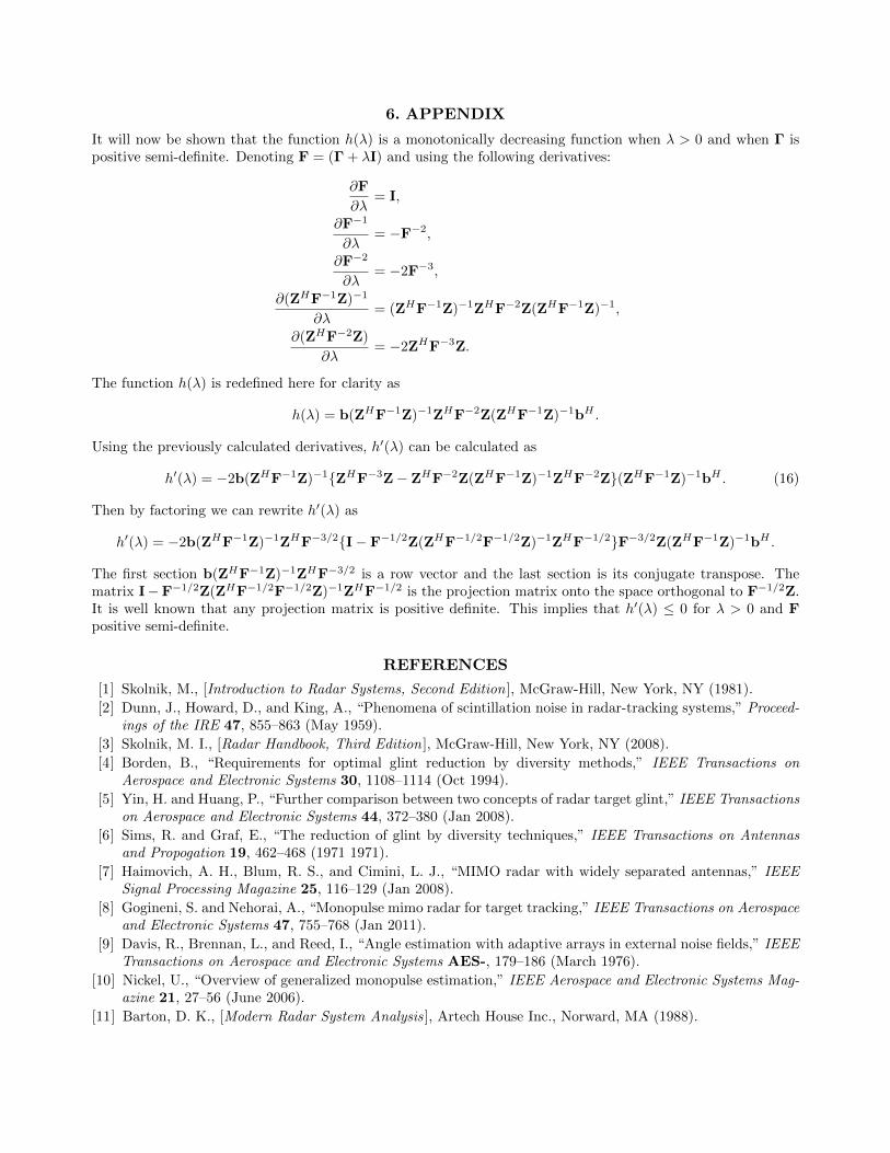
6. APPENDIX

It will now be shown that the function h(λ) is a monotonically decreasing function when λ > 0 and when Γ ispositive semi-definite. Denoting F = (Γ + λI) and using the following derivatives:

∂F

∂λ= I,

∂F−1

∂λ= −F−2,

∂F−2

∂λ= −2F−3,

∂(ZHF−1Z)−1

∂λ= (ZHF−1Z)−1ZHF−2Z(ZHF−1Z)−1,

∂(ZHF−2Z)

∂λ= −2ZHF−3Z.

The function h(λ) is redefined here for clarity as

h(λ) = b(ZHF−1Z)−1ZHF−2Z(ZHF−1Z)−1bH .

Using the previously calculated derivatives, h′(λ) can be calculated as

h′(λ) = −2b(ZHF−1Z)−1{ZHF−3Z− ZHF−2Z(ZHF−1Z)−1ZHF−2Z}(ZHF−1Z)−1bH . (16)

Then by factoring we can rewrite h′(λ) as

h′(λ) = −2b(ZHF−1Z)−1ZHF−3/2{I− F−1/2Z(ZHF−1/2F−1/2Z)−1ZHF−1/2}F−3/2Z(ZHF−1Z)−1bH .

The first section b(ZHF−1Z)−1ZHF−3/2 is a row vector and the last section is its conjugate transpose. Thematrix I−F−1/2Z(ZHF−1/2F−1/2Z)−1ZHF−1/2 is the projection matrix onto the space orthogonal to F−1/2Z.It is well known that any projection matrix is positive definite. This implies that h′(λ) ≤ 0 for λ > 0 and Fpositive semi-definite.

REFERENCES

[1] Skolnik, M., [Introduction to Radar Systems, Second Edition ], McGraw-Hill, New York, NY (1981).

[2] Dunn, J., Howard, D., and King, A., “Phenomena of scintillation noise in radar-tracking systems,” Proceed-ings of the IRE 47, 855–863 (May 1959).

[3] Skolnik, M. I., [Radar Handbook, Third Edition ], McGraw-Hill, New York, NY (2008).

[4] Borden, B., “Requirements for optimal glint reduction by diversity methods,” IEEE Transactions onAerospace and Electronic Systems 30, 1108–1114 (Oct 1994).

[5] Yin, H. and Huang, P., “Further comparison between two concepts of radar target glint,” IEEE Transactionson Aerospace and Electronic Systems 44, 372–380 (Jan 2008).

[6] Sims, R. and Graf, E., “The reduction of glint by diversity techniques,” IEEE Transactions on Antennasand Propogation 19, 462–468 (1971 1971).

[7] Haimovich, A. H., Blum, R. S., and Cimini, L. J., “MIMO radar with widely separated antennas,” IEEESignal Processing Magazine 25, 116–129 (Jan 2008).

[8] Gogineni, S. and Nehorai, A., “Monopulse mimo radar for target tracking,” IEEE Transactions on Aerospaceand Electronic Systems 47, 755–768 (Jan 2011).

[9] Davis, R., Brennan, L., and Reed, I., “Angle estimation with adaptive arrays in external noise fields,” IEEETransactions on Aerospace and Electronic Systems AES-, 179–186 (March 1976).

[10] Nickel, U., “Overview of generalized monopulse estimation,” IEEE Aerospace and Electronic Systems Mag-azine 21, 27–56 (June 2006).

[11] Barton, D. K., [Modern Radar System Analysis ], Artech House Inc., Norward, MA (1988).

[12] Li, J. and Stoica, P., [Robust Adaptive Beamforming ], John Wiley & Sons, New York, NY (2005).

[13] Li, J., Xie, Y., Stoica, P., Zheng, X., and Ward, J., “Beampattern synthesis via a matrix approach for signalpower estimation,” IEEE Transactions on Signal Processing 55, 5643–5657 (December 2007).

[14] Stoica, P. and Moses, R. L., [Spectral Analysis of Signals ], Prentice-Hall, Upper Saddle River, NJ (2005).

[15] CVX Research, I., “Cvx: Matlab software for disciplined convex programming, version 2.0 beta,” (March2013).

chalmers publication...

Documents