cfd analysis of the transonic flow over a naca 0012 airfoil · in this paper, the naca 0012, the...

CFD Analysis of the Transonic Flow over a NACA 0012Airfoil

Analyse CFD de l’écoulement transsonique autour d’un profil d’aileNACA 0012

R. El Maani1, B. Radi2, A. El Hami3

1LSMI, ENSAM Meknès, Marjane 2, Meknès, Morocco, INSA de Rouen, France, [email protected], FST Settat, Maroc, [email protected], INSA de Rouen, France, [email protected]

ABSTRACT. Computational Fluid Dynamics (CFD) incorporates mathematical relations and algorithms to analyze andsolve the problems regarding fluid flow. CFD analysis of an airfoil produces results such as lift and drag forces whichdetermines the ability of an airfoil. In this paper a transonic flow will be modelled over a NACA 0012 airfoil for whichexperimental data has been published, so that a comparison can be made. The flow to be considered is compressible andturbulent and the solver used is the density based implicit solver, which gives good results for high speed compressibleflows. The results show that the predicted lift, drag and pressure cœfficients are in good agreement with experimental data.KEYWORDS. CFD, aerodynamic, NACA 0012, pressure cœfficient, airfoil.

1. Introduction

The rapid evolution of computational fluid dynamics (CFD) has been driven by the need for faster andmore accurate methods for the calculations of flow fields around configurations of technical interest. Inthe past decade, CFD was the method of choice in the design of many aerospace, automotive and indus-trial components and processes in which fluid or gas flows play a major role. In the fluid dynamics, thereare many commercial CFD packages available for modeling flow in or around objects. The computersimulations show features and details that are difficult, expensive or impossible to measure or visualizeexperimentally. When simulating the flow over airfoils, transition from laminar to turbulent flow playsan important role in determining the flow features and in quantifying the airfoil performance such aslift and drag. Hence, the proper modeling of transition, including both the onset and extent of transitionwill definitely lead to a more accurate drag prediction. The first step in modeling a problem involvesthe creation of the geometry and the meshes with a preprocessor. The majority of time spent on a CFDproject in the industry is usually devoted to successfully generating a mesh for the domain geometry thatallows a compromise between desired accuracy and solution cost. After the creation of the grid, a solveris able to solve the governing equations of the problem. The basic procedural steps for the solution of theproblem are the following. First, the modeling goals have to be defined and the model geometry and gridare created. Then, the solver and the physical models are stepped up in order to compute and monitor thesolution. Afterwards, the results are examined and saved and if it is necessary we consider revisions tothe numerical or physical model parameters.

2. Mathematical formulation

For the description of fluid flows usually the Eulerian formulation is employed, because we are usuallyinterested in the properties of the flow at certain locations in the flow domain. We restrict ourselves to the

c© 2018 ISTE OpenScience – Published by ISTE Ltd. London, UK – openscience.fr Page | 1

case of linear viscous isotropic fluids known as Newtonian fluids, which are by far the most importantones for practical applications. Newtonian fluids are characterized by the following material law for theCauchy stress tensor T :

Tij = µ

(∂vi∂xj

+∂vj∂xi− 2

3

∂vk∂xk

δij

)− pδij [1]

with the velocity vector vi with respect to Cartesian coordinate xi, the pressure p, the dynamic viscosityµ, and the Kronecker symbol δij . The Navier-Stokes equations of incompressible flows may be writtenon the spatial fluid mechanics domain as :

(∂v)

∂t+∇ · (ρv ⊗ v − σ)− ρf = 0

∇ · v = 0 [2]

where ρ, v, and f are the density, velocity, and the external force, respectively, and σ the stress tensor isdefined as :

σ(v, p) = −pI + 2µε(v) [3]

Here p is the pressure, I is the identity tensor, µ is the dynamic viscosity, and ε(v) is the strain-rate tensorgiven by :

ε(v) =1

2

(∇v +∇vT

)[4]

The boundary conditions associated to the fluid domain are :

v|Γv = v [5]

where v can be a known velocity profile at the boundary.

3. Turbulence model

In general, turbulence models attempt to modify the original unsteady Navier-Stokes equations byintroducing averaged and fluctuating quantities to produce Reynolds Averaged Navier-Stokes equations(RANS). The turbulence models based on the RANS equations are known as statistical turbulence modelsbecause of the statistical mean procedure used to obtain the equations. In our study the k-Omega SSTmodel will be used [3].


3.1. K-Omega SST model

The shear-stress transport (SST) k − ω model was developed by Menter [9] to effectively blend therobust and accurate formulation of the model in the near-wall region with the freestream independenceof the k − ω model in the far field.

The SST k − ω model has a similar form to the standard k − ω model :

∂

∂t(ρk) +

∂

∂xi(ρkui) =

∂

∂xj

(Γk

∂k

∂xj

)+ G̃k − Yk + Sk [1]

∂

∂t(ρω) +

∂

∂xi(ρωui) =

∂

∂xj

(Γω

∂ω

∂xj

)+Gω − Yω +Dω + Sω [2]

Where Dω represents the cross-diffusion term. The turbulent viscosity µi is computed as follows :

µt =ρk

ω

1

max[

1α∗ ,

SF2

a1ω

] [3]

Where : σk = 1F1σk,1

+(1−F1)σk,2

and σω = 1F1σω,1

+(1−F1)σω,2

. F1 and F2 are the blending functions,

The term G̃k represents the production of turbulence kinetic energy, and is defined as :

G̃k = min (Gk, 10ρβ∗kω) [4]

The term Gω represents the production of and is given by :

Gω =α

νtGk [5]

The SST k − ω model is based on both the standard k − ω model and the standard k − ε model. Toblend these two models together, the standard k− ε model has been transformed into equations based onk and ω, which leads to the introduction of a cross-diffusion term Dω is defined as :

Dω = 2(1− F1)ρσω,21

ω

∂k

∂xj

∂ω

∂xj[6]

Model constants are :

σk,1 = 1.176, σω,1 = 2.0, σk,2 = 1.0, σω,2 = 1.168

a1 = 0.31, βi,1 = 0.075, βi,2 = 0.0828, k = 0.41 [7]


4. Numerical simulation

4.1. Problem statement

In this paper, the NACA 0012, the well documented airfoil from the 4-digit series of NACA airfoils,was utilized. The NACA 0012 airfoil is symmetrical ; the 00 indicates that it has no camber. The 12indicates that the airfoil has a 12% thickness to chord length ratio ; it is 12% as thick as it is long.Mach number for the simulations was evaluated for M = 0.5 and M = 0.7, same with the reliableexperimental data from T.J. Coakley (1987) [9], in order to validate the present simulation. The freestream total temperature is 311 K, which is the same as the environmental temperature. The density ofthe air at the given temperature is ρ = 1.225 kg/m3 and the viscosity is µ = 1.7894×10−5 kg/m.s. Forthis Mach numbers, the flow can be described as compressible. A segregated, implicit solver was utilized(ANSYS/Fluent). Calculations were done for angle of attack α = 1.55◦. The airfoil profile meshes werecreated using structured meshes, which consist of a variety of quadrilateral elements. The resolution ofthe mesh was greater in regions where greater computational accuracy was needed, such as the regionclose to the airfoil.

The first step in performing a CFD simulation should be to investigate the effect of the mesh size onthe solution results. Generally, a numerical solution becomes more accurate as more nodes are used,but using additional nodes also increases the required computer memory and computational time. Theappropriate number of nodes can be determined by increasing the number of nodes until the mesh issufficiently fine so that further refinement does not change the results.

4.2. Boundary conditions

Figure 1. Boundary conditions

• airfoil_lower and airfoil_upper : We will be setting this to a wall boundary condition, setting thevelocity there to be 0.


• inlet, outlet : We will be setting far-field pressure, Mach number, temperature, and components ofthe velocity. This allows for the calculation of the speed of sound, and the velocity direction.

4.3. Results

The main source of experimental data, used here for comparison, are the measured flow parameters onstraight wings, with unchanged cross sections along their span, and collected in the Experimental DataBase for Computer Program Assessment (AGARD-AR-138, 1979) for checking computational fluiddynamic methods. This 12% thick symmetrical airfoil is widely used for testing different computingmethods. The data on the flow over the airfoil are obtained in several wind tunnels, but, according toHoist (1987) [10], it is best to take the data from Harris’s tests in the Langley 8-Foot Transonic PressureTunnel [11]. Computations were performed at a Reynolds number of Re = 9.l06. Comparison of thecomputed results with Harris’s data for the pressure cœfficient are shown in Figures 3 and 5 at M = 0.5

and M = 0.7 at angle of attack α = 1.55◦. Table 1 pressents a comparision of the lift and drag cœfficientswith the experimental data.

Figure 2. Evolution of the drag and lift cœfficients for Mach 0.5

Figure 3. Cp along the upper and lower airfoil surfaces for Mach 0.5


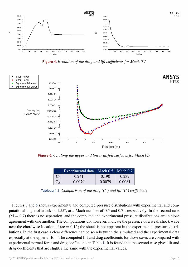
Figure 4. Evolution of the drag and lift cœfficients for Mach 0.7

Figure 5. Cp along the upper and lower airfoil surfaces for Mach 0.7

Experimental data Mach 0.5 Mach 0.7Cl 0.241 0.190 0.239Cd 0.0079 0.0079 0.0081

Tableau 4.1. Comparison of the drag (Cd) and lift (Cl) cœfficients

Figures 3 and 5 shows experimental and computed pressure distributions with experimental and com-putational angle of attack of 1.55◦, at a Mach number of 0.5 and 0.7 , respectively. In the second case(M = 0.7) there is no separation, and the computed and experimental pressure distributions are in closeagreement with one another. The computations do, however, indicate the presence of a weak shock wavenear the chordwise Iocatlon of x/c = 0.15 ; the shock is not apparent in the experimental pressure distrl-butions. In the first case a clear difference can be seen between the simulated and the experimental dataespecially at the upper airfoil. The computed lift and drag coefficients for those cases are compared withexperimental normal force and drag coefficients in Table 1. It is found that the second case gives lift anddrag coefficients that are slightly the same with the experimental values.


5. Conclusion

In this paper ANSYS/FLUENT has been used within a workbench project to compute the transonic,compressible flow over a NACA0012 airfoil. The implicit density based solver with solution steering wasemployed and the computed results have been compared to published experimental data and good agree-ment was achieved. A case comparison has been carried out within CFD Post to compare the pressurefields at Mach 0.5 and Mach 0.7.

Bibliographie

[1] EL HAMI A., RADI B., Fluid-Structure Interactions and Uncertainties : Ansys and Fluent Tool, John Wiley and Sons,2017.

[2] EL MAANI R., Étude Basée Sur l’optimisation Fiabiliste En Aérodynamique, INSA de Rouen, 2016.

[3] LAUNDER B. E., SPALDING D. B., Lectures in Mathematical Models of Turbulence, Academic Press, London, En-gland, 1972.

[4] SOULI M., BENSON D. J., Arbitrary Lagrangian-Eulerian and Fluid-Structure Interaction, ISTE Ltd and John WileySons, 2010.

[5] HUANG S., LI R., LI Q.S., Numerical simulation on fluid-structure interaction of wind around super-tall building athigh reynolds number conditions, Structural Engineering and Mechanics, 46(2) : 197-212, 2013.

[6] PATANKAR S.V., Numerical Heat Transfer and Fluid Flow, Hemisphere Publishing, New York, USA, 1980.

[7] FERZIGER J.H., PERIC M., Computational Methods for Fluid Dynamics, Springer, Berlin, Germany, 1996.

[8] CHOPRA A., Dynamics of Structures, Pearson Prentice Hall, 2nd ed, 2001.

[9] COAKLEY T.J., Numerical Simulation of Viscous Transonic Airfoil Flows, NASA Ames Research Center, AIAA-87-0416, 1987.

[10] HOIST T.L., Viscous transonic airfoil workshop compedium of results, AIAA Paper No. 87-1460, 1987.

[11] HARRIS C.D., Two-Dimensional Aerodynamic Characteristics of the NACA 0012 Airfoil in the Langley 8-foot Trans-onic Pressure Tunnel, NASA Ames Research Center, NASA TM 81927, 1981.


cfd analysis of the transonic flow over a naca 0012 airfoil · in this paper, the naca 0012, the...

Documents