ceriotti, matteo, and mcinnes, colin r. (2014) design of
TRANSCRIPT

Ceriotti, Matteo, and McInnes, Colin R. (2014) Design of ballistic three-body trajectories for continuous polar earth observation in the earth-moon system. Acta Astronautica, 102 . pp. 178-189. ISSN 0094-5765 Copyright © 2014 IAA A copy can be downloaded for personal non-commercial research or study, without prior permission or charge
Content must not be changed in any way or reproduced in any format or medium without the formal permission of the copyright holder(s)
When referring to this work, full bibliographic details must be given http://eprints.gla.ac.uk/94552 Deposited on: 02 July 2014
Enlighten – Research publications by members of the University of Glasgow http://eprints.gla.ac.uk

Page 1 of 23
TITLE
Design of ballistic three-body trajectories for continuous polar Earth observation in the Earth-Moon system
AUTHOR NAMES AND AFFILIATIONS
Matteo Ceriotti
School of Engineering
University of Glasgow
G12 8QQ
Glasgow, United Kingdom
Phone: +44 (0)141 330 6465
(Corresponding author)
Colin R. McInnes
Advanced Space Concepts Laboratory, Department of Mechanical & Aerospace Engineering
University of Strathclyde
75 Montrose Street, James Weir Building
G1 1XJ
Glasgow, United Kingdom
Phone: +44 (0)141 548 2049

Page 2 of 23
ABSTRACT
This paper investigates orbits and transfer trajectories for continuous polar Earth observation in the Earth-Moon
system. The motivation behind this work is to complement the services offered by polar-orbiting spacecraft, which
offer high resolution imaging but poor temporal resolution, due to the fact that they can only capture one narrow
swath at each polar passage. Conversely, a platform for high-temporal resolution imaging can enable a number of
applications, from accurate polar weather forecasting to Aurora study, as well as direct-link telecommunications with
high-latitude regions. Such a platform would complement polar orbiters. In this work, we make use of resonant
gravity swing-by manoeuvres at the Moon in order to design trajectories that are suitable for quasi-continuous polar
observation. In particular, it is shown that the Moon can flip the line of apsides of a highly eccentric, highly inclined
orbit from north to south, without the need for thrust. In this way, a spacecraft can alternatively loiter for an extended
period of time above the two poles. In addition, at the lunar encounter it is possible to change the period of time
spent on each pole. In addition, we also show that the lunar swing-by can be exploited for transfer to a so-called
pole-sitter orbit, i.e. a spacecraft that constantly hovers above one of the Earth’s poles using continuous thrust. It is
shown that, by using the Moon’s gravity to change the inclination of the transfer trajectory, the total Δv is less than
using a trajectory solely relying on high-thrust or low-thrust, therefore enabling the launchers to inject more mass
into the target pole-sitter position.
Keywords: Continuous polar coverage, Earth-Moon system, Gravity assist, Pole-sitter transfer design, Trajectory
design

Page 3 of 23
MANUSCRIPT
1. INTRODUCTION
It is widely known that the polar regions of the Earth cannot be monitored from space in the same way as the low-
latitude and equatorial regions. Due to the Earth’s spin around its polar axis, the equatorial plane offers a useful
vantage-point: a spacecraft in geostationary orbit (GEO) is stationary with respect to an observer on the surface of
the Earth, thus providing a means for data relay and hemispheric imaging in one single frame.
However, the coverage of GEO spacecraft degrades at higher latitudes, because the spacecraft’s elevation angle
becomes very low. Therefore, other platforms are currently being used for polar coverage: they include highly
eccentric orbits (like Molniya [1]), which use the oblateness of the Earth to maintain the argument of the pericentre
constant in time [2]. Their inclination is fixed at a value of 63.4°, which is still relatively low to obtain a satisfactory
coverage of the high-latitude regions [3]. Low- and medium-altitude polar orbits (such as Sun-synchronous orbits)
are also widely used for polar imaging, due to the high spatial resolution that they can provide; however only a
narrow swath is imaged at each polar passage, relying on multiple passages for complete coverage. This results in
poor temporal resolution for the entire polar region, as different areas are imaged at different times, hence missing
the opportunity to have a simultaneous and continuous real-time view of the pole. In other words, spatial resolution
is traded off for temporal resolution.
In this paper, instead, we are interested in studying a platform that offers high temporal resolution, offering a service
that is complementing low and medium Earth orbit spacecraft. The reason for this interest originates in a number of
potential applications that could be enabled by a platform that can continuously cover the poles. Although high-
bandwidth telecommunications and high-resolution imagery are difficult due to the large Earth-spacecraft distance, a
number of novel potential applications are enabled, both in the fields of observation and telecommunications. It was
shown that spatial resolution in the visible wavelength in the range 10-40 km should be sufficient for real-time,
continuous views of dynamic phenomena and large-scale polar weather systems [4]. The creation of atmospheric
motion vectors (AMV) would also make use of the stationary location of the platform, avoiding gap problems related
to geo-location and inter-calibration that composite images introduce [5]. Glaciology and ice-pack monitoring would
also benefit from continuous, but low resolution polar observation [5]. Ultraviolet imagery of the polar night regions
at 100 km resolution or better would enable real-time monitoring of rapidly-changing hot spots in the aurora that can
affect high frequency communications and radar [4]. The platform could also be used as a continuous data-relay for
key Antarctic research activities, in particular for scientific experiments, links to automated weather stations,
emergency airfields and telemedicine. Ship tracking was also proposed, to support future high-latitude oil and gas
exploration [3].
It is clear that the only platform that can offer the same coverage conditions for the poles as a GEO spacecraft would
be a stationary spacecraft aligned with the polar axis. This is known in the literature as a “pole-sitter” or “pole-
squatter”, and has been investigated since 1980, starting from Driver’s analysis [6] up to an end-to-end to end,
optimised mission and systems design performed by the authors [7]. The main disadvantages of this type of
spacecraft is the considerable distance from the Earth, as well as the need for continuous low-thrust in order to

Page 4 of 23
maintain its vantage position, and therefore the mission lifetime is seriously affected by the availability of propellant
mass on-board.
To overcome these limits, other concepts were investigated the literature, including the use of solar sailing [8, 9].
Recently, work performed by the authors investigated alternative mission scenarios in the Sun-Earth system,
including optimisedpole-sitters and periodic high-amplitude vertical Lyapunov orbits [10].
The aim of this paper is to explore possible mission scenarios for continuous polar coverage using periodic
trajectories in the Earth-Moon system. Past studies in the literature showed the possibility of using a gravity assist at
the Moon to change the orbital plane of a spacecraft with respect to the lunar orbital plane [11], without the need of
expensive thrusting manoeuvres. This idea can be exploited for reaching orbits that pass over the Earth’s poles at
little cost, or indeed used for the transfer to the pole-sitter position. The so-called lunar backflip orbits were also
studied in the literature [12, 13], however while one leg of the orbit hovers over a pole of the Earth, the second one
has a very low inclination, therefore not offering any possibility of polar coverage. In this work, we use a patched-
conic approximation to design Earth-centred orbits that exploit the swing-by of the Moon to achieve the desired
orbital elements.
The paper is organised as follows. Initially, the dynamics of the lunar swing-by is explained in Section 2, together
with the two methods that will be used, throughout the work, to solve the resulting velocity triangles. Section 3 then
describes the orbits for polar observation, including a strategy to flip the line of the nodes and therefore observe the
North Pole and the South Pole alternatively, and also change the period of observation of each pole. Section 4
investigates the use of the lunar swing-by to design a transfer to the pole-sitter position, and it includes a preliminary
assessment of the mass that can be injected into the poles-sitter position using Ariane 5 and Soyuz.
2. LUNAR SWING-BY
This section shows the methodology followed to solve the ballistic swing-by at the Moon [14]. We approximate the
Moon’s orbit as a perfectly circular orbit around the Earth, at radius 384,401 kmMr , with velocity M Mv r ,
with 5 3 23.9860 10 km s the planetary gravitational parameter of the Earth.
Let us call v the absolute velocity vector at the Moon, and denote with a superscript “-” the incoming conditions just
before the swing-by manoeuvre, and with “+” the outgoing ones, just after the manoeuvre.
One assumption that is being made, and that will be used throughout the paper, is that in the outgoing orbit, the
anomaly of the pericentre is 2 or 3 2 and the swing-by is at a true anomaly 2 or 3 2 .
Some of these orbits are represented in Fig. 4, for a specific inclination. This also implies that the line of the nodes of
the outgoing orbit coincides with the semi-latus rectum direction, and that the anomaly of the pericentre is either
2 or 3 2 . This translates into the following relation between the outgoing velocity v and the flight path angle
:
22 cosM
M
r vhp r
(1)

Page 5 of 23
arccosM
M
r
r v
(2)
where p is the semi-latus rectum length.
Note that this relationship introduces a constraint on v such that exists; it must be
1M
M
r
r v
or
M
M
v vr
Let us consider a reference frame centred in the Moon, aligned with the radial, transversal and out-of-plane
directions of the Moon’s orbit. In this frame, the velocity of the Moon, purely transversal, is:
0, ,0T
M Mvv
where M Mv r
The incoming relative velocity, at infinity of the swing-by hyperbola, is:
M
v v v (3)
As well known in the literature, a ballistic swing-by does not change the magnitude of the velocity at infinity, but
only its direction. Therefore it is possible to define a constantv sphere around Mv , which represents all
hyperbolas with the same energy around the Moon. The outgoing absolute velocity vector shall stay on this spherical
surface (represented in grey in Fig. 1 and Fig. 2). However, the exact position on the surface is yet to be determined.
Two procedures will be used, depending on whether the outgoing orbit inclination is given, or the semi-major axis.
2.1. Outgoing inclination given
In this case, the inclination of the outgoing orbit is known, therefore the outgoing velocity vector must lie on a plane
that is inclined at i around the radial direction, measured from the Moon’s orbit plane. This plane is in red in Fig. 1.
When an intersection exists, this is a circumference, whose radius is 2
2 sinMCD v v i , and v is on this
circumference (see Fig. 1 for defining points and segments). Instead, if the plane does not intersect the sphere (i.e.
sinMv v i ), then no solution is possible, i.e. either the incoming velocity vector or the outgoing inclination shall
be changed.
In order to define the position of v on the circumference, we introduce a parameterisation through an angle , that
is the angle between the radius defining the vector v and a radius aligned on the radial direction. With this choice,
we have the following outgoing velocity and flight path angle:
2 2
2 2 cos2
v CD AC CD AC
(4)

Page 6 of 23
2 2
2
arccos2
v AC CD
v AC
(5)
However, the flight path angle can also be expressed through Eq. (2). The value of can then be found numerically,
through a line search, by equating Eq. (2) to Eq. (5). Once is known, Eq. (4) and (5) can be used to determine
and v .
Fig. 1. Velocity vectors of the swing-by with outgoing inclination given. Only solution with is represented.
Bold segments are velocity vectors. Dashed segments are velocities relative to the Moon. Blue refers to
incoming vectors, red refers to outgoing vectors. Black vectors refer to the Moon orbit.
2.2. Outgoing semi-major axis given
In this second case, we assume that the semi-major axis of the outgoing orbit is given. Note that, since the semi-latus
rectum of the orbit is fixed, see Eq. (1), equivalently any other in-plane parameter could be provided.
The outgoing absolute velocity magnitude can immediately be computed through the orbital energy:
2
M
vr a
Now Eq. (2) can be used to find the flight path angle . All possible outgoing orbits will differ in inclination, but
have the same and v . This means that all possible v define two conical surfaces around the radial direction (in
red in Fig. 2): each cone spans all possible inclinations of outgoing orbit, and the two cones refer to the two cases
0, 0 . Since the vector v shall also lie on the sphere, then the problem is to find the intersection between
the circumference defining the base of the cone and the sphere. The vector v can be parameterised as a function of
the unknown inclination:
Page 7 of 23
cos
sin cos
cos sin
i v i
i
v (6)
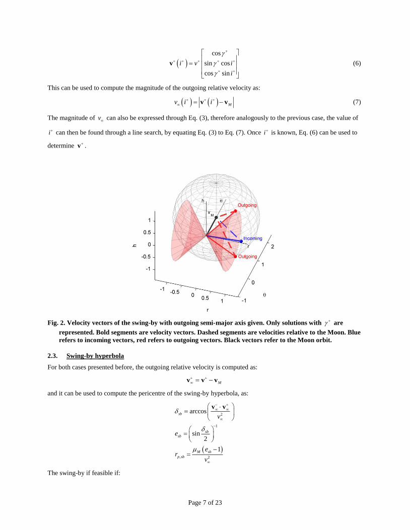
This can be used to compute the magnitude of the outgoing relative velocity as:
Mv i i
v v (7)
The magnitude of v can also be expressed through Eq. (3), therefore analogously to the previous case, the value of
i can then be found through a line search, by equating Eq. (3) to Eq. (7). Once i is known, Eq. (6) can be used to
determine v .
Fig. 2. Velocity vectors of the swing-by with outgoing semi-major axis given. Only solutions with are
represented. Bold segments are velocity vectors. Dashed segments are velocities relative to the Moon. Blue
refers to incoming vectors, red refers to outgoing vectors. Black vectors refer to the Moon orbit.
2.3. Swing-by hyperbola
For both cases presented before, the outgoing relative velocity is computed as:
M
v v v
and it can be used to compute the pericentre of the swing-by hyperbola, as:
2
1
, 2
arccos
sin2
1
sb
sb
sb
M sb
p sb
v
e
er
v
v v
The swing-by if feasible if:

Page 8 of 23
,p sb Mr R (8)
where 1738 kmMR is the radius of the Moon, and the gravitational parameter of the Moon is 3 -24902.8 kg sM .
3. POLAR OBSERVATION ORBITS
In this section, we will devise a strategy for covering both North and South Poles, involving a sequence of lunar
swing-bys to change the orbital parameters.
The lunar orbit is inclined 5.145° to the ecliptic, and due to the precession of the nodes (one revolution every 18.6
years), and the obliquity of the Earth’s equator with respect to the ecliptic of 23.44°, the inclination with respect to
the Earth’s equator varies between 18.29° and 28.58°. For sake of simplicity, in this work it is assumed that this
inclination fixed to 23eqi .
These trajectories are based on the work of Uphoff [15] and Uphoff et al. [11], following a suggestion of Edwin
“Buzz” Aldrin. In that work, the concept of a lunar cycler was described, in which a 180° Moon-to-Moon “backflip”
transfer is used to generate a “lunar cycler” (see Fig. 3, taken from Uphoff et al. [11]): a spacecraft is injected from
Earth into an eccentric orbit targeting the Moon; a lunar swing-by modifies the orbital elements to achieve an orbit
that is inclined (~45°) and encounters the Moon again after half a lunar period; finally, a second lunar swing-by
directs the spacecraft into a planar, eccentric orbit passing close to the Earth.
Fig. 3. 180° Moon-to-Moon backflip transfer, as described by Uphoff et al.[11] [Image taken from the same
source]
In that work, the inclined orbit of the cycler is chosen in order to re-encounter the Moon with some relative velocity.
However, it is interesting to see that such orbits offer polar coverage for a certain amount of time. This time could be
extended by considering orbits with greater semi-major axis, but still such that they re-encounter the Moon at the line
of the nodes. Since the orbit of the Moon is almost circular (and assumed exactly circular in this paper), the two
encounters shall happen at the two points in which the orbit has the same distance from the focus, i.e. the semi-latus
rectum. This also justifies the assumption made in the previous section, where the outgoing orbit anomaly of
pericentre had to be 2 or 3 2 .
In addition, in order to encounter the Moon with the right timing at the node, it is necessary that the following
relationship holds:
2 3 2 0.5 MP t t n P

Page 9 of 23
P represents the time between two lunar encounters, or between the ascending node and the descending node of the
orbit, passing from the apocentre. t is the time at true anomaly , which can be found through the eccentric
anomaly and Kepler’s equation:
1
2arctan tan1 2
eE
e
2
sinM
t E e EP
27.45 dMP is the period of the Moon, and n 0 is an integer that defines the number of resonances with the
Moon, i.e. the number of full revolutions of the Moon between the two lunar encounters.
Table 1 shows the in-plane Keplerian elements for a number of these orbits.
Table 1. Period between lunar passages and in-plane Keplerian elements for orbits resonant with the Moon.
Period between
lunar passages, P
Semi-major
axis, a, 610 km
Eccentricity,
e
0.5 13.726 dMP 0.3844 0
1.5 41.178 dMP 0.5657 0.5662
2.5 68.630 dMP 0.7560 0.7011
3.5 96.082 dMP 0.9273 0.7652
4.5 123.534 dMP 1.0847 0.8035
If coverage of the North and South Pole is needed, then the swing-by of the Moon can be used to rotate the line of
the nodes by 90°, without changing the inclination of the orbit. This means that if the pericentre of the incoming orbit
is on the north side, the outgoing orbit will have its pericentre in the south side. In other words, the pericentre and
apocentre directions are inverted, as illustrated in Fig. 4. In particular, the figure plots, for the orbits in Table 1,
flipped orbits with the same period.
We note that, in the particular case when the incoming and outgoing orbits have the same in-plane orbital elements
and the same inclination, the velocity change required at the lunar swing-by corresponds to a change in sign of the
radial component of the velocity.
Flipping the line of apsides is not always possible with a swing-by of the Moon. Depending on the incoming and
outgoing velocity vectors, the required deflection might be too high, and therefore the constraint (8) is not satisfied.
In order to understand when such a manoeuvre can be done, Fig. 5 shows contours of constant radius of pericentre
,p sbr that is required for such manoeuvre at the Moon, depending on the inclination and the semi-major axis (equal
for both incoming and outgoing orbits). The vertical dashed lines, plotted for convenience, show the semi-major axis
of the orbits with the resonance indicated by the number on the line ( 0.5n ). The black contour line, corresponding
to , 1p sbr represents the bound of the feasible solutions, and shows that a higher inclination is necessary as the
period increases. For example, it is possible to flip the line of apsides of an orbit inclined 40° if 2n , but not if
3n or more.

Page 10 of 23
Fig. 4. Effect of rotation of the line of apsides without changing the other orbital elements, for the orbits in
Table 1, and arbitrary inclination of 67°.
Fig. 5. Pericentre of the swing-by hyperbola (normalised on the lunar radius) necessary to rotate the line of
nodes 90°, depending on the semi-major axis and the inclination of the orbit.
Because of the same incoming and outgoing orbital periods, both the orbits will encounter the Moon each time they
reach the line of the nodes. However, a more general case exists, in which the outgoing orbit does not have the same
period as the incoming one, but just one of the periods listed in Table 1: in this way, there will be again a lunar
encounter at each nodal crossing. Assuming that the incoming orbit has an inclination of 67° (i.e. aligned with polar
axis), and applying the swing-by solution method in Section 2.2, it is possible to find the data in Table 2. For
different periods of the incoming and outgoing orbits, the table shows the inclination of the outgoing orbit. It is worth
noting that, for small changes in inclination, that do not affect the coverage of the pole, it is possible to achieve
substantial changes of the period of the orbit. For example, for an incoming orbit of 2n , the outgoing orbit can
have 4n with just approximately 10° of inclination loss.

Page 11 of 23
Table 2. Outgoing inclination (in deg) for different incoming and outgoing orbital periods between lunar
encounters. Incoming inclination is 67° (aligned with polar axis).
Incoming P Outgoing P
1.5 MP 2.5 MP 3.5 MP 4.5 MP
1.5 MP 67 61.56 58.45 56.40
2.5 MP 72.23 67 64.04 62.11
3.5 MP 75.03 69.89* 67 65.11
4.5 MP 76.81 71.71 68.86 67
These results open the way for different strategies for monitoring the North Pole and the South Pole alternatively. In
fact, at the lunar swing-by, it is possible to decide the period of the next orbit, and therefore the time spent covering
one pole, before switching to the other one.
The natural choice of the north and south orbits would be 6.5 MP P . This corresponds approximately to half a year,
and with the proper synchronisation with the Sun, it would be possible to cover both the North Pole and the South
Pole when illuminated by the Sun, in a similar fashion to what proposed by Heiligers et al. [16] Observing the pole
when lit is particularly important, as it enables the acquisition of imagery in the visible band of the spectrum, which
in turn provides essential data for meteorology and glaciology [3]. Unfortunately, the choice of 6.5 MP P is not
advisable, for two reasons: the first is that, for this orbit, no feasible swing-by exists to rotate the line of apsides; the
second is that, due to its semi-major axis length, the orbit goes far away from the Earth, and the two-body
approximation would start to become incorrect.
Fig. 6 and Fig. 7 and show one combination of north-south orbits, which is the one with an asterisk in Table 2 (in
inertial and synodic frames respectively). The figure shows the trajectory in an inertial frame and in an Earth-Moon
synodic frame. The translucent conical surface in Fig. 7 is the one described by the apparent rotation of the polar axis
(which is inertially fixed) in the synodic reference. Both plots allow appreciate the difference in semi/major axis (and
thus period) between the north and the south orbit, despite the inclination is very similar.

Page 12 of 23
Fig. 6. Plot of trajectory (in Earth-centred inertial frame) with north orbit at 67°, 3.5 MP P , and south orbit
at to 69.89°, 2.5 MP P . The lunar swing-by provides the manoeuvre to change the orbital elements.
b)
Fig. 7. Same as Fig. 6, in Earth-Moon synodic frame.
3.1. Continuous coverage analysis
With the aim of showing the coverage offered by the orbits, and in particular to show the continuous coverage of the
polar regions, we consider the same figure of merit introduced in Ceriotti et al. [3] Referring to the geometry in Fig.
8, we define a minimum elevation angle of the spacecraft, min . The spacecraft, at latitude , is in sight of a point
on the Earth’s surface only if its elevation angle is min . This angle defines a circular area centred in the sub-
satellite point, such that any observer in this area is in sight of the spacecraft, at a given instant of time (yellow
shaded area in Fig. 8). However, assuming that the motion of the spacecraft is much slower than the Earth’s rotation
around its axis, then it might happen that, due to the Earth’s rotation, some points that at some time during the day
are accessible, become inaccessible at some other time. Therefore the green area in Fig. 8 is defined by the latitude Λ
above which any point on the Earth is in sight of the spacecraft, at any time of the day (i.e. for any angular position
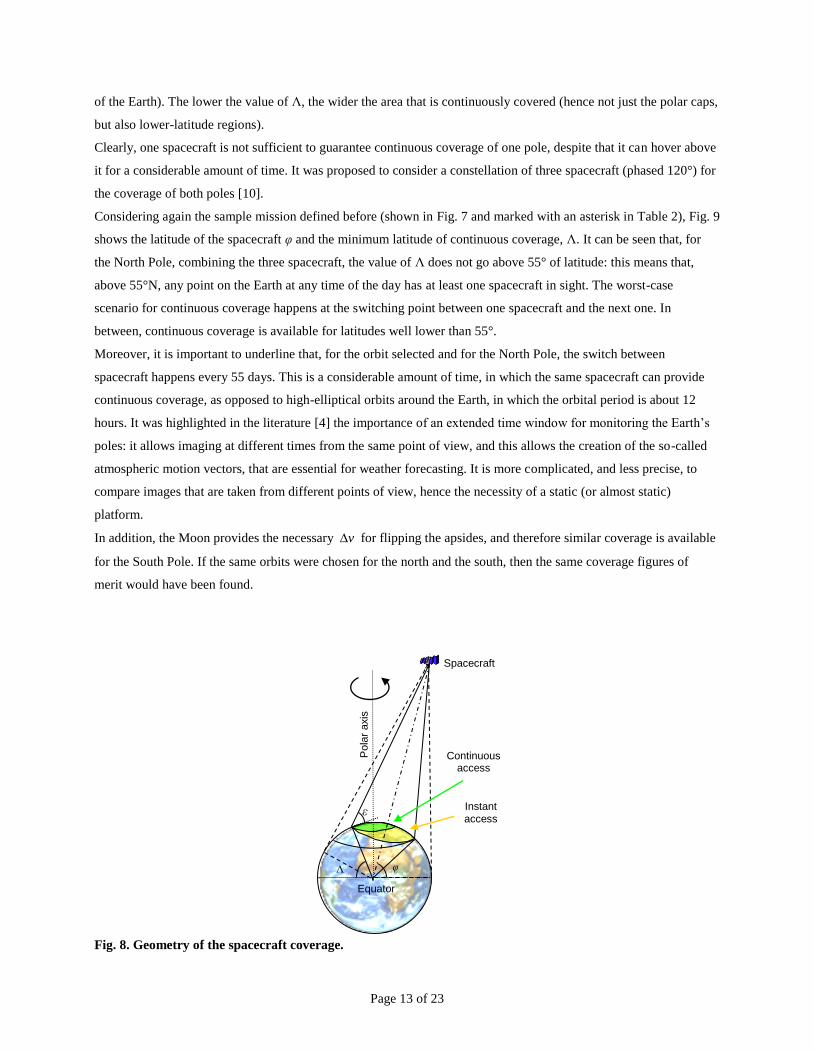
Page 13 of 23
of the Earth). The lower the value of Λ, the wider the area that is continuously covered (hence not just the polar caps,
but also lower-latitude regions).
Clearly, one spacecraft is not sufficient to guarantee continuous coverage of one pole, despite that it can hover above
it for a considerable amount of time. It was proposed to consider a constellation of three spacecraft (phased 120°) for
the coverage of both poles [10].
Considering again the sample mission defined before (shown in Fig. 7 and marked with an asterisk in Table 2), Fig. 9
shows the latitude of the spacecraft φ and the minimum latitude of continuous coverage, Λ. It can be seen that, for
the North Pole, combining the three spacecraft, the value of Λ does not go above 55° of latitude: this means that,
above 55°N, any point on the Earth at any time of the day has at least one spacecraft in sight. The worst-case
scenario for continuous coverage happens at the switching point between one spacecraft and the next one. In
between, continuous coverage is available for latitudes well lower than 55°.
Moreover, it is important to underline that, for the orbit selected and for the North Pole, the switch between
spacecraft happens every 55 days. This is a considerable amount of time, in which the same spacecraft can provide
continuous coverage, as opposed to high-elliptical orbits around the Earth, in which the orbital period is about 12
hours. It was highlighted in the literature [4] the importance of an extended time window for monitoring the Earth’s
poles: it allows imaging at different times from the same point of view, and this allows the creation of the so-called
atmospheric motion vectors, that are essential for weather forecasting. It is more complicated, and less precise, to
compare images that are taken from different points of view, hence the necessity of a static (or almost static)
platform.
In addition, the Moon provides the necessary v for flipping the apsides, and therefore similar coverage is available
for the South Pole. If the same orbits were chosen for the north and the south, then the same coverage figures of
merit would have been found.
Fig. 8. Geometry of the spacecraft coverage.
ε
Pola
r axis
Equator
Spacecraft
Continuous access
φ Λ
Instant access

Page 14 of 23
Fig. 9. Coverage figures for three spacecraft on trajectory represented in Fig. 7. (a) Latitude φ; (b) Angle Λ.
Both functions of time during the mission.
4. TRANSFER TO POLE-SITTER ORBIT
Breakwell et al. [17] presented a low-thrust transfer to a pole-sitter (in that work, named “pole-squatter”), which
basically consisted in a transfer to a highly inclined, highly eccentric Earth orbit. The same idea is used in this work,
where a preliminary approximation of the transfer to the pole-sitter position can be done by considering a highly
eccentric orbit, the apocentre of which coincides with the pole-sitter position. However, we will also consider a
breaking manoeuvre at the apocentre. This is due to the fact that this manoeuvre can have a non-negligible effect on
the overall v of the transfer. Consequently, the inclination of this orbit over the Earth’s equator shall be 90°.
In previous studies, this inclination was achieved either through a set of impulsive manoeuvres performed by the
launcher main stage and/or upper stage [18], or (partly) by the low-thrust propulsion system of the spacecraft [17,
18]. However, it is well known that launcher performances are higher when the target orbit is equatorial (assuming
the availability of an equatorial launch site). Therefore, it is worth investigating whether a gravity assist at the Moon
can provide the necessary inclination change, in a way that the total cost of the transfer is less, and therefore more
mass can be injected into the pole-sitter orbit, for the same mass injected into a LEO parking orbit by the launcher.
4.1. Transfer design
We consider a transfer strategy that relies on a single gravity assist of the Moon. Referring to Fig. 10, we assume a
launcher with the capability of injecting a spacecraft and an upper stage into a circular equatorial LEO around the
Earth. The upper stage then provides an impulsive manoeuvre LEOv that transfers the spacecraft into a coplanar
orbit (named incoming orbit) that encounters the Moon. Parameters of this orbit will be denoted with a superscript (-)
because they refer to the orbit before the swing-by manoeuvre. The manoeuvre is:
2
1LEO
LEO LEOLEO
vr rr e
where 200 kmLEOr is set arbitrarily and the eccentricity of the incoming orbit e is to be determined. Note that
the minimum eccentricity to reach the Moon is:

Page 15 of 23
0.9664M LEO
min
M LEO
r re
r r
when the Moon is at the apocentre of the incoming orbit.
At the Moon, the swing-by is resolved using the method in Section 2.1. Figure 11 shows contour lines of constant
outgoing inclination, function of the incoming orbit eccentricity and outgoing orbit apocentre. The graph is limited in
the upper-left region by the feasibility condition of the swing-by (Eq. (8)).
Fig. 10. Illustration of the transfer to the pole-sitter.
Fig. 11. Contours of constant inclination of outgoing orbit (in deg), function of incoming eccentricity and
outgoing apocentre radius.
For the transfer under consideration, the inclination of the outgoing orbit is known: 90 67eqi i , such that the
apocentre is on the polar axis of the Earth. In addition, since we are interested in a North-Pole transfer, the argument
Earth polar axis
Line of nodes
Moon’s orbit
Moon swing-by
Pole-sitter position
Earth’s equatorial
plane
eqi
90 eqi
Incoming orbit
Outgoing orbit

Page 16 of 23
of pericentre is 270°, and 0 . The spacecraft orbit after the swing-by, or outgoing orbit, is therefore determined
in terms of ,a e (function of e ). This corresponds to the bold contour line in Fig. 11.
The apocentre of the outgoing orbit, ar , is chosen to match the pole-sitter position. However, it is necessary to
consider a final braking manoeuvre av at the apocentre
ar :
2
a
a
vr a
Due to the geometry of the orbits considered, and in particular the eccentricity being less than unity, the magnitude
of this manoeuvre can be sensible. Conversely, in other types of transfers not involving the lunar swing-by [17], the
eccentricity reaches values of approximately 1, and therefore this manoeuvre is negligible.
Note that, following this manoeuvre, a constant thrust is necessary to maintain the position, as discussed in previous
work [19]. However, this is not part of the transfer, and therefore it will not be discussed here.
The total v for the transfer from LEO is therefore:
LEO av v v (9)
Fig. 12 shows contour lines for the total v , parameterised as in the previous Fig. 11. The black transversal contour
line represents solutions in which 67i .
Fig. 13 shows the total v , as well as the two contributions as in Eq. (9), for the specific case under consideration of
67i . This figure can be imagined as a section of Fig. 11 along the contour line. Note that the manoeuvre at LEO
increases very slowly with the apocentre of the target orbit, instead the magnitude of the manoeuvre at the apoapsis
decreases rapidly. This makes it more economical to reach a steady pole-sitter position that is farther from the Earth,
within the considered range of apocentre distances.
Fig. 12. Total Δv (as from Eq. (9)) function of function of incoming eccentricity and outgoing apocentre radius.

Page 17 of 23
Fig. 13. Total Δv for reaching a stationary pole-sitter position, starting from a 200 km altitude circular
equatorial orbit at the Earth.
We consider two pole-sitter mission profiles, corresponding to two different altitudes of the spacecraft. The first one,
injects the satellite to 0.01 AU, that is 61.496 10 km , the second to 62.5 10 km . These two values are taken from
the description of the poles-sitter mission [19], and the first is the distance of a constant-altitude reference mission,
while the second is the average distance of a minimum-propellant hybrid or SEP pole-sitter mission.
By fixing the apogee ar , the incoming eccentricity e can also be found, and the transfer is fully determined. Plots
of the orbits used in the transfer are in Fig. 14 for the two different distances. Note that although the full orbit is
plotted, the spacecraft would only follow part of it during the transfer. Table 3 summarises the results for the two
transfers.
Note that we assumed that the LEO is equatorial, and so is the incoming orbit. However, no launcher option of those
considered here are equatorial, but their inclination is up to about 8° over the equator. It can be shown that small
inclination changes do not change the results considerably. An inclination change in the incoming orbit corresponds
to a rotation of the incoming velocity vector v around the radial direction. Since the transversal and out-of-plane
components of the vector are small compared to the radial one, it results that a change in inclination does not affect
the lunar swing-by considerably, and consequently the total v of the transfer.

Page 18 of 23
a) b)
Fig. 14. The two orbits used in the transfer, patched by the lunar swing-by: incoming (blue) and outgoing
(red) orbits. The dashed black line shows the polar axis of the Earth. (a) 61.496 10 kmar ;
(b) 62.5 10 kmar .
Table 3. Details of transfers from LEO to two different distances of the pole-sitter.
Distance
ar , km
Swing-by pericentre
,p sbr , km Total v ,
km/s 61.496 10 km 4040 km 3.4441 km/s
62.5 10 km 4020 km 3.3467 km/s
4.2. Launcher performance
Given the trajectory and total velocity change required to transfer from LEO to the pole-sitter, in this section we
provide an estimation of the mass that can be injected into the pole-sitter, considering two launcher options: Ariane 5
ECA and Soyuz CSG (launching from Kourou, French Guyana). The same launchers were considered in previous
work, although the launch strategy was based on a sequence of impulses and/or low-thrust arcs in order to achieve
the pole-sitter position, instead of a lunar swing-by. This will allow to compare the mass injected into pole-sitter
orbit with that work, as a reference.
For both launchers, the manuals do not provide information for injection in the exact orbit computed in the previous
section, therefore we will estimate the required data assuming impulsive manoeuvres of the upper stage, that join a
circular LEO around the Earth to the target orbit.
In particular, the manual provides the total injected mass m into a given orbit ,a e . We now assume that the
injection into this orbit is performed from a circular LEO orbit, and therefore the impulsive velocity change can be
computed as:
2
LEO LEO
vr r a

Page 19 of 23
This velocity change is provided by the upper stage of the launcher platform. The total mass that can be injected into
LEO by the launcher (which includes propellant, upper stage, adapter and payload):
0 sp
v
g I
LEO usm m m e
where usm is the mass of the upper stage and its adapter, and
spI its specific impulse, as provided in Table 4.
Since the total v for the transfer to the pole-sitter is known, and assuming again that the upper stage is providing
the entire velocity change, then we can compute the injected mass into the pole-sitter position:
0 sp
v
g I
ps LEO usm m e m
Table 4. Upper stage characteristics.
Launcher Sp. impulse spI , s Mass
usm , kg
Soyuz 330 1100
Ariane 5 446 4700
4.2.1. Soyuz CSG
For computing the deliverable mass by the Soyuz, we refer to the manual [20] where the performance (kg) is shown
as a function of the altitude of the perigee of the target orbit. The perigee is at 250 km, and the inclination to 6°.
Since the inclination is low, and as noted before does not affect considerably the v , inclination changes are
neglected here. The plot, taken from the manual, is reproduced in Fig. 15. It can be seen that the graph does not
include altitude of apocentre above 80,000 km. Therefore, we take the GTO reference, where we have:
42.4753 10 km
0.7322
a
e
Applying the previous formulas it is found that Soyuz can inject 2101 kg at 0.01 AU and 2199 kg at 62.5 10 km .
Fig. 15. Performance of Soyuz (kg of payload) for elliptic orbits (function of apogee altitude) with low
inclination. [Figure from Soyuz User’s Manual [20]]
4.2.2. Ariane 5
The Ariane 5 manual does not provide a plot similar to that in Fig. 15 for Soyuz. Instead, some reference target orbits
are listed as typical mission profiles [21]. The most similar profile is the “injection towards the Moon”, for which

Page 20 of 23
7000 kg can be inserted into an orbit with apogee and perigee altitude of 385,600 km and 300 km respectively. This
corresponds to:
51.9933 10 km
0.9665
a
e
The orbit is also inclined 12°, but again this does not affect the arrival velocity at the Moon considerably. In fact, an
equatorial launch could possibly improve the performance of the launcher.
Using these values, it results that 6135 kg and 6379 kg can be injected in the near and far pole-sitter positions,
respectively.
4.2.3. Summary
Table 5 shows a summary of the results in terms of mass that can be injected into two different pole-sitter positions.
As a reference, it was found in previous work [18] that, by using the same launchers in combination with solar
electric propulsion, the mass that can be injected into pole-sitter is about 1450 kg with Soyuz and 4450 kg with
Ariane 5, with very small variations for different altitude of the injection point.
It shall be underlined that, although these results provide an indication of the mass that can be injected into the pole-
sitter orbit, they cannot be directly compared to what is found in Heiligers et al. [18], because in that work, in the last
part of the transfer the effect of the gravitational attraction of the Sun was taken into account. On the other hand, if
SEP were employed for these types of transfer, it could be that the v for braking at the apogee would be distributed
in a low-thrust arc that starts just after the lunar swing-by. The gravity losses of a distributed thrust arc would
presumably increase the necessary v , but the higher specific impulse of the solar electric propulsion (of the order
of 3000 s, one order of magnitude bigger than what offered by the upper stages) could indeed compensate, possibly
allowing overall propellant saving.
In addition, the lunar swing-by increases considerably the complexity of the transfer, in terms of spacecraft
operations, mainly due to the accuracy that is necessary for targeting the Moon, and due to the intrinsic risk of the
swing-by manoeuvre (missing the correct hyperbola would almost certainly bring the spacecraft on a non-
recoverable path).
All these issues shall be taken in a trade-off with the additional spacecraft mass that the lunar swing-by makes
potentially available.
Table 5. Mass injected into pole-sitter position, mps, kg.
Distance, ar Ariane 5 Soyuz
61.496 10 km 6135 2101 62.5 10 km 6379 2199
5. CONCLUSION
This work has shown the capabilities offered by the lunar swing-by manoeuvre for generating trajectories for polar
Earth observation, resonant with the Moon. It was shown that the Moon can be used to flip the line of apsides of an
eccentric, highly-inclined orbit, enabling the possibility to switch between north and south coverage at no cost. With

Page 21 of 23
small changes in inclination, it is also possible to modify the resonances with the Moon, therefore changing the time
spent on each pole.
The swing-by of the Moon was also used to generate transfers to the pole-sitter orbit, and it was shown that, at the
cost of additional complexity due to the swing-by, more mass could be injected into pole-sitter position.
Third body effects were not considered in this work, however some of the proposed orbits reach significant distances
from the Earth, and therefore is it expected that the perturbation of the Sun would become important. Additional,
future studies are necessary to quantify the corrections necessary to keep the spacecraft on-track, both in the case of
elliptic orbits for Earth observation, and transfers to pole-sitter.
ACKNOWLEDGEMENTS
This work was conceived as part of European Research Council project 227571 VISIONSPACE, at the University of
Strathclyde.
REFERENCES
[1] P.C. Anderson, M. Macdonald, Extension of the Molniya orbit using low-thrust propulsion, 21st AAS/AIAA
Space Flight Mechanics Meeting, AIAA, New Orleans, USA, 2011.
[2] J.R. Wertz, W.J. Larson, Space mission analysis and design, third edition, Space technology library, Microcosm
press/Kluwer Academic Publishers, El Segundo, California, USA, 1999.
[3] M. Ceriotti, B.L. Diedrich, C.R. McInnes, Novel mission concepts for polar coverage: an overview of recent
developments and possible future applications, Acta Astronaut, 80 (2012) 89-104. DOI:
10.1016/j.actaastro.2012.04.043.
[4] M.A. Lazzara, A. Coletti, B.L. Diedrich, The possibilities of polar meteorology, environmental remote sensing,
communications and space weather applications from Artificial Lagrange Orbit, Adv Space Res, 48 (2011) 1880-
1889. DOI: 10.1016/j.asr.2011.04.026.
[5] C.R. McInnes, P. Mulligan, Final report: telecommunications and Earth observations applications for polar
stationary solar sails, National Oceanographic and Atmospheric Administration (NOAA)/University of Glasgow,
Department of Aerospace Engineering, 2003.
[6] J.M. Driver, Analysis of an arctic polesitter, J Spacecraft Rockets, 17 (1980) 263-269. DOI: 10.2514/3.57736.
[7] M. Ceriotti, J. Heiligers, C.R. McInnes, Novel pole-sitter mission concepts for continuous polar remote sensing,
SPIE Remote Sensing, Edinburgh, United Kingdom, 2012. DOI: 10.1117/12.974604.
[8] T.J. Waters, C.R. McInnes, Periodic orbits above the ecliptic in the solar-sail restricted three-body problem, J
Guid Control Dynam, 30 (2007) 687-693. DOI: 10.2514/1.26232.
[9] R.L. Forward, Statite: a spacecraft that does not orbit, J Spacecraft Rockets, 28 (1991) 606-611. DOI:
10.2514/3.26287.
[10] M. Ceriotti, C.R. McInnes, Natural and sail-displaced doubly-symmetric Lagrange point orbits for polar
coverage, Celest Mech Dyn Astr, 114 (2012) 151-180. DOI: 10.1007/s10569-012-9422-2.
[11] C. Uphoff, M.A. Crouch, Lunar cycler orbits with alternating semi-monthly transfer windows, Advances in the
Astronautical Sciences, 75 (1991) 163-170.

Page 22 of 23
[12] P. Pergola, Low-thrust transfer to backflip orbits, Adv Space Res, 46 (2010) 1280-1291. DOI:
10.1016/j.asr.2010.06.018.
[13] D.J. Dichmann, E.J. Doedel, R.C. Paffenroth, The computation of periodic solutions of the 3-body problem
using the numerical continuation software AUTO, International Conference on Libration Point Orbits and
Applications, Aiguablava, Spain, 2002.
[14] M.H. Kaplan, Modern spacecraft dynamics and control, John Wiley and Sons, Inc., New York, 1976.
[15] C. Uphoff, The art and science of Lunar gravity assist, AAS/GSFC International Symposium on orbital
Mechanics and Mission Design, NASA-GSFC, USA, 1989.
[16] J. Heiligers, M. Ceriotti, C.R. McInnes, J.D. Biggs, Design of optimal transfers between North and South pole-
sitter orbits, 22nd AAS/AIAA Space Flight Mechanics Meeting, Univelt, inc., Charleston, South Carolina, USA,
2012.
[17] J.V. Breakwell, O.M. Golan, Low thrust power-limited transfer for a pole squatter, AIAA/AAS Astrodynamics
Conference, AIAA, Minneapolis, MN, USA, 1988, pp. 717-722.
[18] J. Heiligers, M. Ceriotti, C.R. McInnes, J.D. Biggs, Design of optimal Earth pole-sitter transfers using low-
thrust propulsion, Acta Astronaut, 79 (2012) 253–268. DOI: 10.1016/j.actaastro.2012.04.025.
[19] M. Ceriotti, C.R. McInnes, Generation of optimal trajectories for Earth hybrid pole-sitters, J Guid Control
Dynam, 34 (2011) 847-859. DOI: 10.2514/1.50935.
[20] Arianespace, Soyuz User's Manual - Issue 2 Revision 0, Arianespace, 2012.
[21] Arianespace, Ariane 5 User's Manual - Issue 5 Revision 1, Arianespace, 2011.

Page 23 of 23
Vitae
MATTEO CERIOTTI
Dr. Matteo Ceriotti received his M.Sc. summa cum laude from Politecnico di Milano (Italy) in 2006 with a thesis on
planning and scheduling for planetary exploration. In 2010, he received his Ph.D. on “Global Optimisation of
Multiple Gravity Assist Trajectories” from the Department of Aerospace Engineering of the University of Glasgow
(United Kingdom). During 2009-2012, Matteo was a research fellow at the Advanced Space Concepts Laboratory,
University of Strathclyde, Glasgow, leading the research theme “Orbital Dynamics of Large Gossamer Spacecraft”.
In 2012, he returned to the University of Glasgow as a lecturer in Space Systems Engineering, within the School of
Engineering. His main research interests are space mission analysis and trajectory design, orbital dynamics,
trajectory optimisation, particularly focusing on high area-to-mass ratio structures.
COLIN MCINNES
Colin McInnes is Director of the Advanced Space Concepts Laboratory at the University of Strathclyde. His work
spans highly non-Keplerian orbits, orbital dynamics and mission applications for solar sails, spacecraft control using
artificial potential field methods and is reported in over 150 journal papers. Recent work is exploring new
approaches to spacecraft orbital dynamics at extremes of spacecraft length-scale to underpin future space-derived
products and services. McInnes has been the recipient of awards including the Royal Aeronautical Society Pardoe
Space Award (2000), the Ackroyd Stuart Propulsion Prize (2003) and a Leonov medal by the International
Association of Space Explorers (2007).