Centre for

Financial Risk _____________________________________________________________________________________________________

An Analytical Real Option Framework for Catastrophic Losses

Mitigation Investment under Climate Change

Chi Truong and Stefan Trück

Working Paper 11-03

The Centre for Financial Risk brings together researchers in the Faculty of Business & Economics on

uncertainty in capital markets. It has two strands. One strand investigates the nature and

management of financial risks faced by institutions, including banks and insurance companies, using

techniques from statistics and actuarial science. It is directed by Associate Professor Ken Siu. The

other strand investigates the nature and management of financial risks faced by households and by

the economy as a whole, using techniques from economics and econometrics. It is directed by

Associate Professor Stefan Trück. The co-directors promote research into financial risk, and the

exchange of ideas and techniques between academics and practitioners.

1

An Analytical Real Option Framework for

Catastrophic Losses Mitigation Investment

under Climate Change

Chi Truong

Department of Economics, Macquarie University, Sydney

Tel. (02) 98508481

Fax: +612 9850 8586

Email: chi.truong@mq.edu.au

Stefan Trück

Department of Applied Finance and Actuarial Studies,

Macquarie University, Sydney

Tel. (02) 98508483

Fax: +612 9850 8586

Email: stefan.trueck@mq.edu.au

2

Abstract

It is of significant concern that climate change will exaggerate the frequency and severity of

extreme events such as floods, storms, droughts and bushfires. As the value of properties under

risk increases due to economic and population growth and the probability of catastrophic events

increases under climate change, there is a need for local governments to evaluate adaptation

measures that reduce potential losses from these catastrophes. Previous studies have mostly

examined only static adaptation strategies, i.e. adapt now or never adapt. For studies that examine

optimal adaptation timing, numerical dynamic programming computation is required, making it

costly to evaluate adaptation strategies and difficult to get insights into factors that affect the value

of adaptation projects. In this paper, a framework that links the Loss Distribution Approach often

used in insurance modelling with real option theory is provided. The closed functional form for the

option to invest enables easy computation of the optimal investment rule. Empirical results for a

bushfire management project show that ignoring the flexibility of the adaptation decision as in

previous studies may result in significant losses or nonoptimal timing of investments.

Keywords: Real option, Catastrophic Risk, Climate Change, Adaptation.

3

1. Introduction

It is a major concern that global warming will make the climate system more

energetic and increase the frequency and the severity of catastrophic events. The

concern has received increasingly more attention when the occurrence of disasters

became more frequent over the last two decades (van Aalst 2006). Given the long

life of greenhouse gases and the long time horizon required for the global climate

system to cool down once being heated, current mitigation efforts may only

reduce catastrophic risks in the far future. The global temperature is going to

increase before it stabilizes, even if substantial emission reduction is committed

(IPCC 2007). The risks related to catastrophic events are expected to increase

regardless of mitigation efforts, making climate change adaptation an essential

task.

This paper is concerned with the problem of mitigating the losses from

catastrophes such as bushfires, floods, drought or hurricanes under climate change

scenarios. An important characteristic of the problem is the recurrence of

catastrophes and catastrophic losses. For a given region, after a catastrophe has

occurred, damaged properties may be repaired and when another catastrophe

occurs, another damage to the same property could be caused. Furthermore, the

frequency of catastrophic losses follows an upward trend due to climate change

impacts. The severity of catastrophic losses is also expected to increase over time

due to population and wealth growth in the considered region. An appropriate

evaluation of investment projects that mitigate catastrophic losses over many time

periods needs to incorporate these features.

The problem of evaluating catastrophic losses under climate change is of

significant interest and has been investigated by a number of studies. West et al.

(2001) examine the increased storm damage due to sea level rise in coastal

regions taking into account the option to exit from the risk prone area. Waters et

al (2003) evaluate retrofit options for a storm drainage system in Ontario to adapt

to more extreme rainfalls under climate change. Brouwer and van Ek (2004)

4

evaluate the benefits and costs of a floodplain restoration strategy (widening and

deepening floodplain) that increases the resilience of water systems and reduces

the risks and damages associated with flooding in the Netherlands under climate

change. Suarez et al. (2005) evaluate the productivity loss in the Boston Metro

area due to lack of transportation in flood events caused by climate change.

Kirshen et al. (2008a) evaluate adaptation strategies to reduce the loss from

increased storm surge flooding due to climate change in metropolitan Boston.

Kirshen et al. (2008b) examine strategies to adapt infrastructure systems in urban

areas, recognising that these systems are physically close to each other and

catastrophes that cause failures in one system often have spill-over effects in other

systems. Michael (2007) evaluates the costs of inundation and flooding subject to

sea level rise in a coastal region in Maryland. Zhu et al. (2007) explore the

optimal investment strategy for drainage capacity expansion to protect a

floodplain in California under climate change. Finally, Symes et al. (2009)

examine land retreat strategies in South East Queensland to avoid losses from

storm surge.

In all studies, except for West et al. (2001), simulation techniques are used to

compute the expected loss in a region over a future period of time. Usually, a

climate model is used to generate simulated time series of future climate variables

for the studied region, which are then used as inputs to a vulnerability model

developed by insurance companies to generate losses. While such an approach

makes use of the knowledge about the current development in the region, this

knowledge becomes less relevant when a farther future is considered. The

disadvantage of the approach is that with the use of a complex climate simulation

model, it is difficult to get insights into factors that have critical impacts on

adaptation decisions. Sensitivity analysis can only be carried out with significant

costs due to the intensive computational requirements of the approach. Given the

limit of current scientific knowledge about climate change, great uncertainty

exists regarding the results of climate models. Therefore, sensitivity analysis with

respect to climate change impacts seems indispensible for the users of climate

change adaptation studies.

5

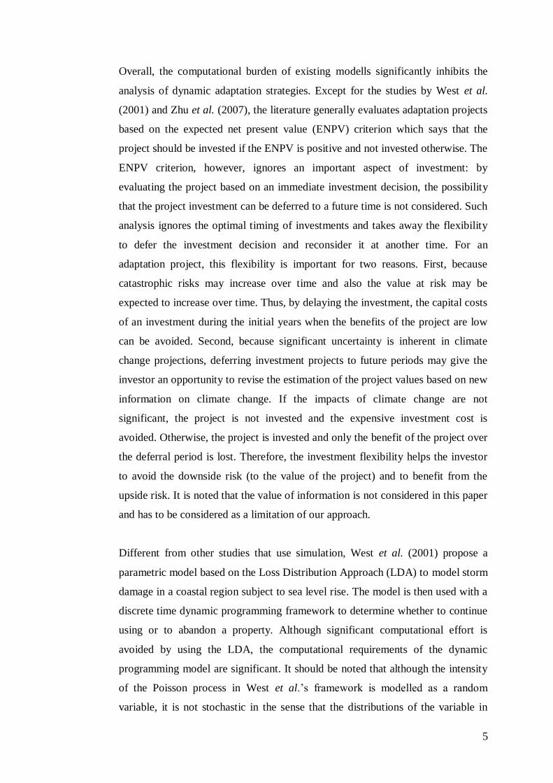
Overall, the computational burden of existing modells significantly inhibits the

analysis of dynamic adaptation strategies. Except for the studies by West et al.

(2001) and Zhu et al. (2007), the literature generally evaluates adaptation projects

based on the expected net present value (ENPV) criterion which says that the

project should be invested if the ENPV is positive and not invested otherwise. The

ENPV criterion, however, ignores an important aspect of investment: by

evaluating the project based on an immediate investment decision, the possibility

that the project investment can be deferred to a future time is not considered. Such

analysis ignores the optimal timing of investments and takes away the flexibility

to defer the investment decision and reconsider it at another time. For an

adaptation project, this flexibility is important for two reasons. First, because

catastrophic risks may increase over time and also the value at risk may be

expected to increase over time. Thus, by delaying the investment, the capital costs

of an investment during the initial years when the benefits of the project are low

can be avoided. Second, because significant uncertainty is inherent in climate

change projections, deferring investment projects to future periods may give the

investor an opportunity to revise the estimation of the project values based on new

information on climate change. If the impacts of climate change are not

significant, the project is not invested and the expensive investment cost is

avoided. Otherwise, the project is invested and only the benefit of the project over

the deferral period is lost. Therefore, the investment flexibility helps the investor

to avoid the downside risk (to the value of the project) and to benefit from the

upside risk. It is noted that the value of information is not considered in this paper

and has to be considered as a limitation of our approach.

Different from other studies that use simulation, West et al. (2001) propose a

parametric model based on the Loss Distribution Approach (LDA) to model storm

damage in a coastal region subject to sea level rise. The model is then used with a

discrete time dynamic programming framework to determine whether to continue

using or to abandon a property. Although significant computational effort is

avoided by using the LDA, the computational requirements of the dynamic

programming model are significant. It should be noted that although the intensity

of the Poisson process in West et al.’s framework is modelled as a random

variable, it is not stochastic in the sense that the distributions of the variable in

6

future periods depends on the realization of the variable in the past. In other

words, West et al.’s framework can be considered as a deterministic framework.

In what follows, we will propose an approach that is similar to West et al.’s

framework to help decision makers at the local level to evaluate projects that

mitigate catastrophic risks under climate change. We formulate the problem in

continuous time and use real option theory to determine the value of the option to

invest and the optimal investment rules. The advantage of our framework is that it

provides a closed functional form, making the calculation of optimal investment

rules easy. In the remainder of the paper, the modeling framework is outlined and

analysed in Section 2. In Section 3, the model is applied to the case of bushfire

risk management in a local region. Conclusions and suggestions for future work

are provided in Section 4.

2. Modeling framework

In this section, a theoretical framework for the analysis of climate change

adaptation options with respect to the risk from catastrophic events is presented.

In a first step, the LDA is extended to quantify potential losses from extreme

events like storms, droughts or bushfires that might be further increased in

frequency and severity due to climate change impacts. Then, in the second step,

the expected value of an adaptation project based on the LDA is used in a real

option framework to determine the optimal investment strategy.

2.1 The Loss Distribution Approach

The LDA is quite popular in the financial industry for modelling insurance claims

and losses arising from operational or catastrophic risks in the banking industry

(see e.g. Klugman et al.(1998)). The approach models the total loss over a period

(0, ]t using a compound Poisson process:

7

( )

1

N t

t n

n

S X , (1)

where tN denotes a homogenous Poisson process with intensity 0 , and

nX is

the loss caused by the nth

catastrophic event. In this standard model, it is assumed

that nX is independently and identically distributed according to a distribution

( )F X and nX is independent from

tN .

The standard model (1) can be extended to examine the current problem as

follows. To allow for increasingly frequent catastrophes, tN

is assumed to follow

a non-homogeneous Poisson process with intensity ( ) 0t . To allow also for

growth of the value of the properties at risk, the catastrophic loss nX is modeled

as the product of the catastrophic loss under zero growth 0X and a growth

component:

0n

nX X e . (2)

In Equation (2), is the growth rate of the value at risk, n is the random time

when the nth event occurs, which is determined by the Poisson process, as later

shown in Lemma 1. The random variable 0X

is the catastrophic loss when the

value of the properties at risk does not grow over time or equivalently, it is the

catastrophic loss that would have been caused if a catastrophic event occurred at

time zero. It is assumed that 0X

is identically, independently distributed

according to a distribution ( )H X and 0X

is independent from

tN and therefore

n.

For the non-homogeneous Poisson process, over a small time interval ( , ]t t t ,

the probability of one loss event occurring is ( )t t and over a time interval

(0, ]t , the probability of having n events is:

8

( )( )Pr{ ( ) }

!

n M tM t eN t n

n, where

0( ) ( )

t

M t u du . (3)

We assume that under climate change, the probability that a catastrophic event

occurs during a small time interval grows at a rate :

( ) (0) tt e . (4)

A property of the Poisson process (3) is that the expected number of events

occuring over any period (0, ]t is equal to parameter ( )M t :

{ ( )} ( )E N t M t .

Using the expression of ( )t in Equation (4), we get:

0( ) ( )

t

M t u du

(0)( 1) /te . (5)

Thus, the expected number of events that occur over any time period 1 2( , ]t t can

be denoted by:

2 1 2 1

2 1

{ ( ) ( )} { ( )} { ( )}

( ) ( )

E N t N t E N t E N t

M t M t

2 1 (0)( ) /t te e (6)

2.2 Investment model

In this section, a framework is presented to evaluate an adaptation project that

reduces the probability of properties in a catastrophe prone region being damaged

when a catastrophic event occurs. As in many previous studies (Suarez et al.

2005; Kirshen et al. 2008a; Brouwer and van Ek 2004; Michael 2007; West et al.

9

2001; Zhu et al. 2007), the decision maker is assumed to be risk neutral. This

assumption is reasonable for investment projects funded by governments since

catastrophic risks in different regions are independent and the government can

pool these risks such that only the expected values are relevant (Kousky et al.

2006).

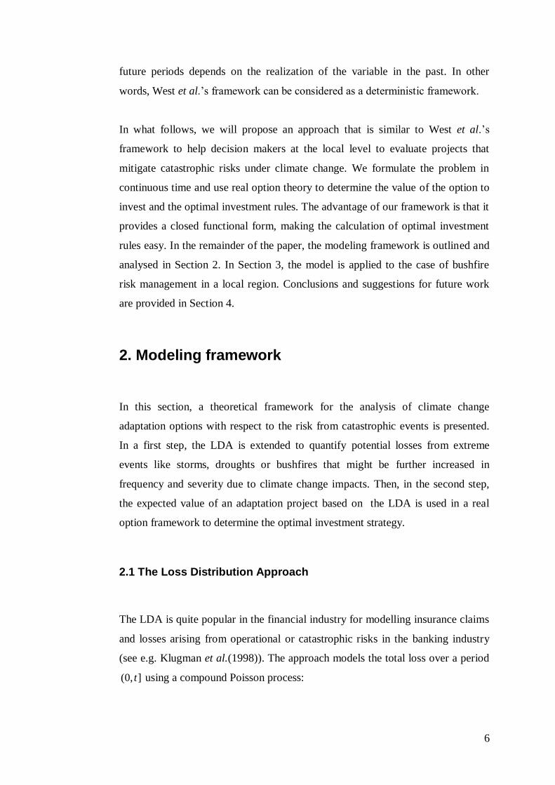
It is assumed that the project reduces the probability of the property at risk being

damaged in a catastrophic event by a proportion k. With the project in place, the

number of damaging events in period t follows a Poisson process with intensity

(1 ) ( )k t . Assume, as in other real options studies, that the investment decision

can be deferred forever, but once the project is invested, a new project will be

invested whenever the old one is fully depreciated (Dixit and Pindyck 1994;

Gollier and Treich 2003; Pindyck 2002; Baranzini et al. 2003; Fisher 2000). Then,

once the project is invested at time T, the catastrophic intensity rate is reduced by

a proportion k for the period ( , )T . To calculate the optimal investment rule, it is

necessary to calculate firstly the value of the project if invested at any time T and

then the value of the option to invest.

2.2.1 Value of the project invested at T

To calculate the value of the project, it is necessary to calculate the total expected

discounted value of losses over the period [ , )T that will be denoted by ˆ( , )S T

in the following. Note that ˆ( , )S T is the sum of the expected discounted value of

all losses , nT

J . Let ( , )ng T be the density function of the random time n when

the nth

catastrophe occurs, with the count of catastrophes starts from time T. Then

ˆ( , )S T can be calculated as:

,1

ˆ( , )nT

n

S T J

10

1

( )

0

1

( )

0

1

{ }

( ) { }

( ) ( , )

n

n

n

n

r

n

r

n

r

n nT

n

E e X

E X E e

E X e g T d

( )

0

1

( ) ( , )nr

n nT

n

E X e g T d . (7)

The density function for the random time n is given in Lemma 1 below.

Lemma 1

Let { }nbe the increasing sequence of all jump times of the non-homogeneous

Poisson process { ( )}N t over time period ( , )t s . The random variable n has the

density:

1

( )( )

( , ) ( )( 1)!

s

t

ns

u dut

n

u du

g t s s en

.

Proof: See Appendix.

Using Lemma 1, the sum 1

( , )n

n

g T in Equation (7) can be simplified:

1

( )

1 1

( )

( , ) ( )( 1)!

T

n

u duT

n

n n

u du

g T s en

1

( )

1

( )

( )( 1)!

T

n

u du T

n

u du

s en

. (8)

Since

1

1

( )

( 1)!

n

T

n

u du

n is the McLaurin series expansion of

( )T

u du

e

(Tchuindjo 2007 p.25), Equation (8) can be rewritten as:

11

( ) ( )

1

( , ) ( ) ( )T Tu du u du

n

n

g T s e e s . (9)

Substituting (9) into (7) leads to:

( )

0ˆ( , ) ( ) ( )r v

TS T E X e v dv (10)

Using the functional form of ( )v given in Equation (4), Equation (10) can be

rewritten as:

( )

0ˆ( , ) ( ) (0)r v v

TS T E X e e dv

( )

0(0) ( ) r v

TE X e dv

( )

0(0) ( ) /( )r TE X e r . (11)

Thus, we have now derived an expression for the total expected discounted value

of losses over the period [ , )T that can be used to calculate the value of an

adaptation project and to find the optimal timing of an investment into such a

project.

2.2.2 The value of the option to invest

With the value of the project at time T being ˆ( ) ( , )V T kS T , the value of the

investment opportunity if executed at time T is:

ˆ( ) ( , ) rTF T kS T e I

( )

0 (0) ( ) /( )r T rTk E X e r e I , (12)

12

where I is the investment cost. The value of the investment opportunity is highest

when the time to invest is optimally chosen. The first order condition for

optimality is:

( ) / 0F T T or:

( )

0(0) ( ) Tk E X e dt rIdt (13)

Equation (13) states that at the optimal time to invest, the marginal benefit of

deferring the investment by a small time period dt must be equal to the marginal

cost of doing so. In Equation (13), the right hand side is the benefit of deferring

the project investment by one period, which is the interest expense on the

investment cost of the project that would have incurred if the project was invested

instantly. The left hand side is the marginal cost of investment deferral, which is

the expected loss that would be avoided should the project be in place. The

marginal cost of deferral grows at a rate equal to the sum of the growth rate of the

catastrophic risk and the growth rate of the value at risk. Because the investment

decision depends only on the sum ( ) of these two parameters, the distinction

between whether the total catastrophic loss in the region is due to increasing

catastrophic risk or due to increasing value at risk is not important. The theory of

optimal investment timing is relevant as long as the total catastrophic loss grows,

regardless of the causes.

From Equation (13), the optimal time to invest is:

*

0

1log

( ) (0) ( )

rIT

k E X. (14)

The condition that makes it optimal to invest immediately can be found by setting

* 0T :

0(0) ( )k E X rI , (15)

which gives:

*(0) /( )V rI r I . (16)

13

That is, it is only optimal to invest immediately if the value of the project at time

zero is greater or equal to *(0)V . As shown in Equation (16), the project should

be invested only when the value of the project exceeds a critical level that is

higher than the investment cost. Investing when the value of the project is just

equal to the investment cost as stipulated by the ENPV criterion is not optimal.

The value of the opportunity to invest at time zero given the current value of the

project (0)V that is lower than *(0)V can be calculated by substituting (14) into

(12):

/( )( (0)) [( ) /( )] ( ) (0) /

rF V I r r V rI (17)

In summary, the value of the opportunity to invest ( )F V is given by:

/( ) *

*

[( ) /( )] ( ) / for ( )

for

rI r r V rI V V

F VV I V V

(18)

3 Empirical results

The model is applied to the case of bushfire management in the Ku-ring-gai

Council area, located on the North Shore of Sydney in New South Wales,

Australia. The region is an urban area that has residential properties being in close

proximity to bushland. The area ranks third with respect to bushfire vulnerability

among the 61 local government areas in the Greater Sydney Region and the risk

of bushfires is predicted to be further amplified by climate change. Therefore, the

increasing frequency and intensity of bushfires is one of the five main concerns of

the local community regarding climate change impacts (Chen 2005).

As a possible adaptation strategy, the risk of house damage could be reduced by

building new fire trails allowing for controlled hazard reduction burning,

breaking wild fire transition and potentially allowing more time for fire brigades

14

to respond to bushfires. To investigate the reduction of the risk for residential

properties, expert opinions could be used to calibrate the parameters of the loss

distributions before and after implementing this adaptation measure. In the

following, the method to estimate parameters is outlined and the results on

optimal investment rules are presented.

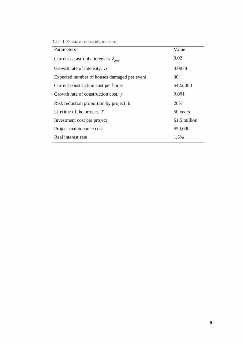
3.1 Parameter Estimation

Parameters of the problem are assumed to take values specified in Table 1. The

process of intensity is estimated as follows. Under the current climate, it is

estimated by the expert that a catastrophe occurs every 50 years, or equivalently,

0.02 catastrophes for one year. With (1) 0.02M , Equation (5) becomes:

(0)( 1) / 0.02e . (19)

Furthermore, for our study we assume that the intensity of catastrophes is going to

double by the year 2100. Using Equation (4), we obtain:

90 89(0)( ) / 0.04e e (20)

Dividing (20) by (19) side by side, we get

90 89( ) /( 1) 2e e e ,

which yields 0.0078 . Substituting into Equation (19) gives (0) 0.02 .

In Table 1, the expected number of houses being damaged in a bushfire event is

also based on expert estimations. The estimated construction cost is calculated by

subtracting the average land value per property estimated by the NSW Valuer

General (DOL 2009) for the Ku-ring-gai region from the average property sales

price for the same region that was used by Hatzvi and Otto (2008). The real

growth rate of construction cost and the real discount rate are estimated by

15

subtracting the inflation rate from the corresponding nominal rate. The real cost of

house construction is estimated from the nominal growth rate of construction cost

estimated using the Price Index of Materials Used in House Building for NSW

over the period 1967-2009 (ABS 2010) subtracted by the inflation rate. The

inflation rate is estimated using the Consumer Price Index over the period 1970-

2009 (RBA 2010). The estimated real growth rate of the construction cost is found

to be 0.1%. The discount rate is assumed to be the social discount rate since the

considered project is invested by the public sector. It is assumed to be 1.5% (see

e.g. Gollier (2008) for the discussion on social discount rate under climate

change). The investment cost is estimated for a project that lasts 50 years.

PLACE TABLE 1 HERE

The estimated costs for a finite lifetime project provided by the expert can be used

to calculate the investment cost of an infinite lifetime project as follows. Let TI be

the estimated investment cost for a project that lasts T years and A be the annuity

of the investment cost, i.e:

11

...1 (1 ) 1

T

TT

A AA A I

r r,

where 1

1 r is the discount factor. Therefore, A can be calculated as

1

1

1T T

A I

such that the investment cost over the infinite time horizon is:

(1 ) /I A r r . (21)

Thus, for building bushfire trails with an investment cost of $1.5 million per

project and yearly project maintenance cost of $50,000, the investment cost

16

equivalent to the flow of cost over the infinite time horizon given by the expert is

$6.2 million.

3.2 Baseline Analysis

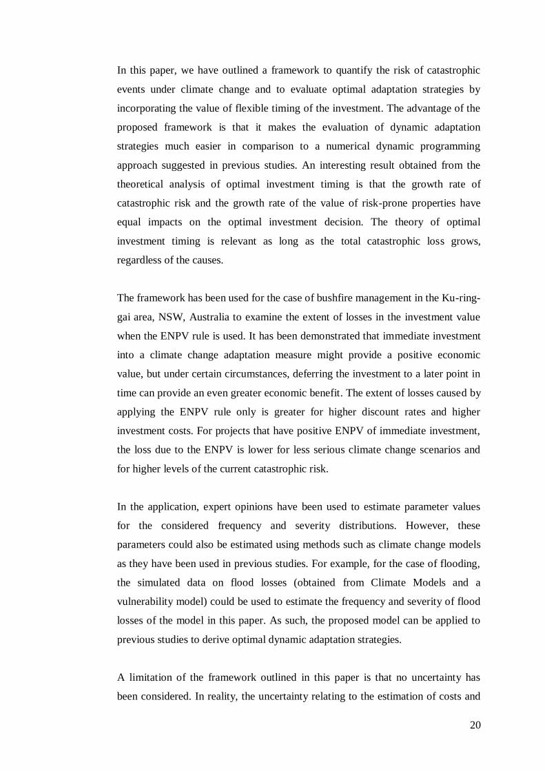
For the assumed values of parameters, the expected net present values of the

project for various investment times are depicted in Figure 1. Immediate

investment provides a value of $1.96 million, but deferring the project to a later

time provides an even higher value. The optimal time to invest as indicated by

Equation (14) is year 69 and investing according to this optimal rule will provide

a value of $3.12 million. If the ENPV rule was used to guide the investment

decision, a value of more than $1 million would be lost.

PLACE FIGURE 1 HERE

3.3 Sensitivity analysis

To examine the robustness of the empirical results, we carry out sensitivity

analysis on four of the major factors having impacts on value of the investment:

the discount rate, the investment cost, the growth rate of catastrophic risk and the

estimation of current catastrophic risk.

Discount rates

The debate on a choice between a social discount rate and a market discount rate

is yet to be settled in the literature (Kuik et al. 2006). In the case of using a market

discount rate, the discount rate will be significantly higher than for the base case

scenario considered in our example. Under a higher discount rate, the capital cost

avoided by deferring the investment increases. With the marginal benefit of

deferring the investment increases, the waiting time to invest increases. The value

of the project for each investment time, however, decreases, which results in a

reduction of the investment option value.

17

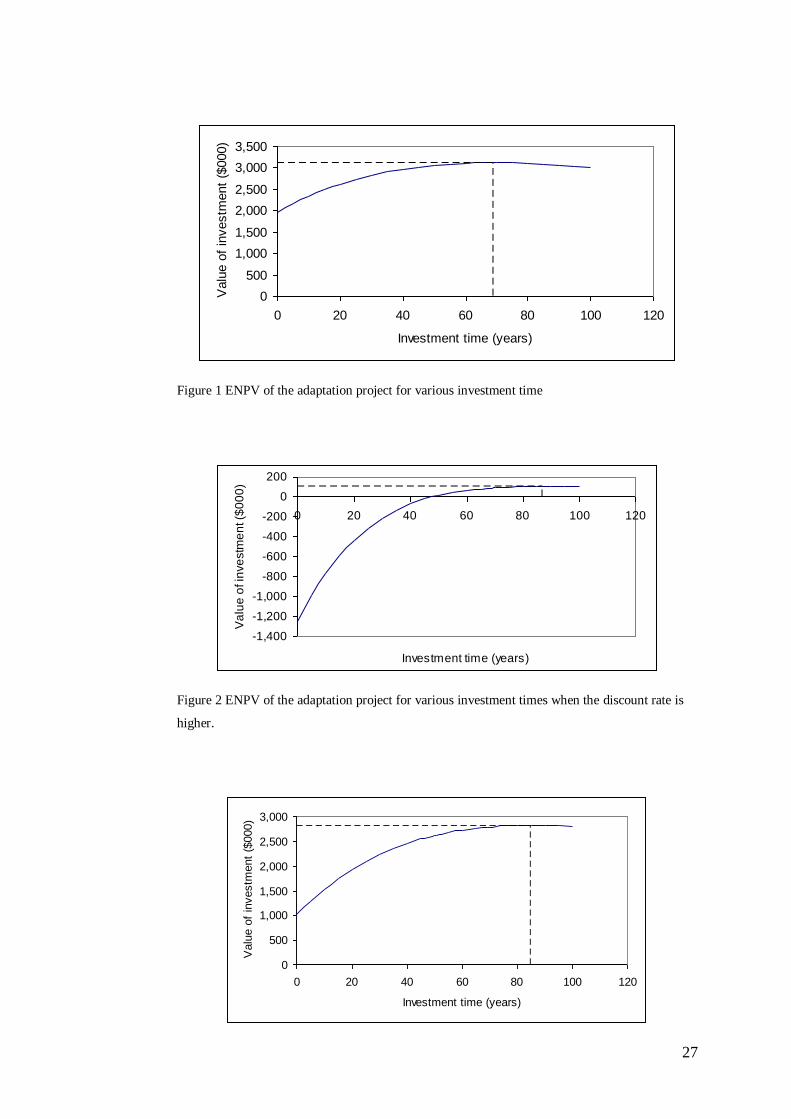
The impacts of an increase of the discount rate to 3% on the ENPV of the project

are shown in Figure 2. An increase in the discount rate has driven the ENPV of an

immediate investment into the project to a negative level, and according to a

simple ENPV rule, the opportunity to invest is worthless. The value of the option

to invest has been reduced, but remains positive. The ENPV rule, therefore, can

mistakenly turn down valuable projects.

The greater impacts of the discount rate increase on the ENPV of an immediate

investment into the project compared to the impacts on the investment opportunity

value can be explained as follows. In calculating the ENPV of the project, a

higher discount rate reduces the value of the project while it leaves the investment

cost unchanged. In contrast, when optimal investment timing is considered, an

increase in the discount rate also reduces the investment cost if the optimal

investment decision is to invest in a future time. As indicated in Equation (14),

increases in the discount rate will increase the waiting time, which reduces the

present value of the investment cost even further. The flexibility to defer the

investment operates as a cushion to reduce the impacts of increases in the discount

rate. As a result, the value of the investment option is reduced by a lesser extent

(from $3.12 million to $0.11 million) compared with the value of the project

under the ENPV rule (from $1.9 million to -$1.25 million).

Overall, higher discount rates increase the difference between the value of the

project obtained from immediate investment and the value obtained when

optimally timing the investment. Therefore, for those levels of discount rates

where the ENPV of the project remains positive, a higher discount rate implies an

even greater loss caused by the ENPV rule in comparison to optimally timing the

investment.

PLACE FIGURE 2 HERE

Investment costs

The impacts of an increase in the investment cost by one third are illustrated in

Figure 3. Increases in the investment cost have similar impacts as those of

increases in the discount rate. As a result of the increase in the investment cost,

18

both the ENPV of the project and the option value decrease, but the loss due to the

usage of the ENPV rule has increased to $1.8 million. Due to discounting, an

increase in the investment cost reduces the value of immediate investment more

than the value of the optimal investment at a future time. The implication is that

dynamic investment strategies or optimal timing of the investment are more

important for projects that have higher investment costs.

PLACE FIGURE 3 HERE

Seriousness of climate change

The future of climate is deeply uncertain due to the uncertainty about future CO2

emissions, and also the values of parameters used by scientists in forecasting

climate change. As indicated in many climate change studies, the impacts of

climate change may become serious much earlier than 2100. To explore this

possibility, we examine the case when climate change results in a doubling of the

catastrophe intensity by 2060, corresponding to an increase in the value of

parameter from 0.0078 in the baseline scenario to 0.0132. The impacts of the

more serious climate change scenario on the ENPVs of investment are presented

in Figure 4.

PLACE FIGURE 4 HERE

As can be seen from Figure 4, under a more serious climate change scenario, the

value of the adaptation project grows faster and the loss caused by the ENPV rule

becomes smaller. This seems to be counter-intuitive because a positive growth in

the value of the adaptation project is what makes investment deferral to be

optimal in the first place. The relationship between the loss caused by the ENPV

rule and the growth rate x of the adaptation project value is in fact non-

linear (Figure 5). For the growth rate that is close to zero, the value of the project

is small and the ENPV of the project is negative. The ENPV rule is to abandon the

project and the loss is equal to the option value of the investment opportunity. As

the growth rate increases, the option value increases and the loss increases. When

the growth rate is sufficiently large so that the ENPV of the project is positive, the

loss due to the ENPV rule is equal to the option value minus the ENPV of

19

immediate investment. Increases in the growth rate in the region where the ENPV

of the project is positive will increase both the option value and the ENPV of the

project with the impacts on the ENPV of the project being larger. As a result, the

loss caused by using the ENPV rule instead of optimal investment time decreases

in this region. The loss is largest when the growth rate is at the level where the

ENPV of the project is zero. For the current problem, this level of growth rate is

0.0068.

PLACE FIGURE 5 HERE

Estimate of current catastrophic intensity

The rule for optimal investment is based on the estimation of the current value of

the project. If the current value of the project, (0)V , is higher than the threshold

*(0)V in Equation (16), the project should be invested. The current value of the

project, however, depends on the estimation of the current catastrophic intensity,

which may be uncertain. The sensitivity of the option value and the ENPV of the

project with respect to the estimate of the current catastrophic intensity (0) is

depicted in Figure 6.

It can be seen that the option value and the ENPV of the project are both convex

in (0) , which means that these values are more sensitive to higher values of

(0) . Also, the relationship between the loss caused by the ENPV rule and (0)

is similar to the relationship between the loss and the growth rate of the project

value. As can be seen from Figure 6, the loss is increasing in (0) when the

ENPV of the project is non-positive and decreasing in (0) when the ENPV is

positive.

PLACE FIGURE 6 HERE

4. Conclusion

20

In this paper, we have outlined a framework to quantify the risk of catastrophic

events under climate change and to evaluate optimal adaptation strategies by

incorporating the value of flexible timing of the investment. The advantage of the

proposed framework is that it makes the evaluation of dynamic adaptation

strategies much easier in comparison to a numerical dynamic programming

approach suggested in previous studies. An interesting result obtained from the

theoretical analysis of optimal investment timing is that the growth rate of

catastrophic risk and the growth rate of the value of risk-prone properties have

equal impacts on the optimal investment decision. The theory of optimal

investment timing is relevant as long as the total catastrophic loss grows,

regardless of the causes.

The framework has been used for the case of bushfire management in the Ku-ring-

gai area, NSW, Australia to examine the extent of losses in the investment value

when the ENPV rule is used. It has been demonstrated that immediate investment

into a climate change adaptation measure might provide a positive economic

value, but under certain circumstances, deferring the investment to a later point in

time can provide an even greater economic benefit. The extent of losses caused by

applying the ENPV rule only is greater for higher discount rates and higher

investment costs. For projects that have positive ENPV of immediate investment,

the loss due to the ENPV is lower for less serious climate change scenarios and

for higher levels of the current catastrophic risk.

In the application, expert opinions have been used to estimate parameter values

for the considered frequency and severity distributions. However, these

parameters could also be estimated using methods such as climate change models

as they have been used in previous studies. For example, for the case of flooding,

the simulated data on flood losses (obtained from Climate Models and a

vulnerability model) could be used to estimate the frequency and severity of flood

losses of the model in this paper. As such, the proposed model can be applied to

previous studies to derive optimal dynamic adaptation strategies.

A limitation of the framework outlined in this paper is that no uncertainty has

been considered. In reality, the uncertainty relating to the estimation of costs and

21

benefits of adaptation projects is vast. Therefore, deferring the investment will

enable the investor to gain more accurate climate change impact assessments. The

value of information will enhance the value of investment flexibility and it might

become even more important to incorporate the value of investment flexibility in

the cost benefit analysis. The extension of the framework to allow for uncertainty

about the growth of value at risk and the impacts of climate change on

catastrophic risks is left for future research.

22

Appendix:

Lemma 1

Let { }nbe the increasing sequence of all jump times of the non-homogeneous

Poisson process { ( )}N t over time period ( , )t s . The random variable n has the

density:

1

( )( )

( , ) ( )( 1)!

s

t

ns

u dut

n

u du

g t s s en

. (22)

Proof:

The proof for the case of homogeneous Poisson processes has been provided by

Shreve (2004 pp. 463-465). The method will be extended for the current problem.

By the definition of the Poisson process, the probability of having n events over

the period (t, s] is:

( )1Pr[ ( ) ( ) ] ( )

!

s

t

ns u du

tN s N t n u du e

n. (23)

Using Equation (23), for n = 0:

( )

1Pr[ ] Pr[ ( ) ( ) 0]

s

tu du

s N s N t e

and the cumulative probability function of 1

is:

( )

1 1( ) 1 Pr[ ] 1

s

tu du

G s s e .

The density function of 1

is then:

( )

1 ( ) ( )

s

tu du

g s s e .

Suppose that Equation (22) holds for some value of n, we need to prove that it

holds for n + 1. We have:

Pr[ ( ) ( ) ] Pr[ ( ) ( ) ] [ ( ) ( ) ]

= Pr[ ( ) ( ) 1] [ ( ) ( ) ]

N s N t n N s N t n N s N t n

N s N t n N s N t n

1Pr[ ] Pr[ ]n ns s

1 1[1 ( )] [1 ( )] ( ) ( )n n n nG s G s G s G s ,

which gives:

1( ) ( ) Pr[ ( ) ( ) ]n nG s G s N s N t n

23

( )1 ( ) ( )

!

s

t

ns u du

nt

G s u du en

(24)

Differentiate Expression (24) with respect to time s:

1( ) ( )

1

1 1( ) ( ) ( ) ( ) ( ) ( )

( 1)! !

s s

t t

n ns su du u du

n nt t

g s g s s u du e s u du en n

Substitute the expression for ( )ng s into the above equation gives:

( )

1

1( ) ( ) ( )

!

s

t

ns u du

nt

g s s u du en

.

24

Acknowledgements

The methodology proposed in this paper was developed in the context of project “Optimal

adaptation and mitigation strategies to climate change for local government”. We would like to

thank the Faculty of Business and Economics at Macquarie University and Macquarie University’s

New Staff Grant funding body for the financial support towards the project.

25

References

ABS, Australian Bureau of Statistics (2010) 6427.0 Producer Price Indexes, Australia. Canberra

Baranzini A, Chesney M, Morisset J (2003) The impact of possible climate catastrophes on global

warming policy. Energ Policy 31 (8):691-701.

Brouwer R, van Ek R (2004) Integrated ecological, economic and social impact assessment of

alternative flood control policies in the Netherlands. Ecol Econ 50 (1-2):1-21.

Chen K Counting bushfire-prone addresses in the Greater Sydney region. In: Proceedings of the

Symposium on Planning for Natural Hazards: how can we mitigate the impacts?, University of

Wollongong, 2-5 February 2005.

Dixit AK, Pindyck RS (1994) Investment under uncertainty. Princeton University Press, Princeton,

New Jersey

DOL, Department of Land (2009) Land values issued for Ku-ring-gai.

Fisher AC (2000) Investment under uncertainty and option value in environmental economics.

Resour Energy Econ 22 (3):197-204.

Gollier C (2008) Discounting with fat-tailed economic growth. J Risk Uncertainty 37 (2-3):171-

186.

Gollier C, Treich N (2003) Decision-making under scientific uncertainty: The economics of the

precautionary principle. J Risk Uncertainty 27 (1):77-103.

Hatzvi E, Otto G (2008) Prices, Rents and Rational Speculative Bubbles in the Sydney Housing

Market. Econ Rec 84 (267):405-420.

IPCC (2007) Climate Change 2007 : the physical science basis: Contribution of Working group I

to the Fourth Assessment Report of the Intergovernmental Panel on Climate Change. Cambridge

University Press, Cambridge ; New York

Kirshen P, Knee K, Ruth M (2008a) Climate change and coastal flooding in Metro Boston:

impacts and adaptation strategies. Climatic Change 90 (4):453-473.

Kirshen P, Ruth M, Anderson W (2008b) Interdependencies of urban climate change impacts and

adaptation strategies: a case study of Metropolitan Boston USA. Climatic Change 86 (1-2):105-

122.

Klugman SA, Panjer HH, Willmot GE (1998) Loss models : from data to decisions. Wiley series

in probability and statistics. Applied probability and statistics. Wiley, New York

Kousky C, Luttmer EFP, Zeckhauser RJ (2006) Private investment and government protection. J

Risk Uncertainty 33 (1-2):73-100.

Kuik OJ, Bucher B, Catenacci M, Karakaya E, Tol RSJ (2006) Methodological aspects of recent

climate change damage cost studies. Fridtjof Nansen Institute, Oslo and Research Unit for

Sustainability and Global Change, Hamburg University,

Michael JA (2007) Episodic flooding and the cost of sea-level rise. Ecol Econ 63 (1):149-159.

Pindyck RS (2002) Optimal timing problems in environmental economics. Journal of Economic

Dynamics & Control 26 (9-10):1677-1697.

G2 CONSUMER PRICE INDEX (2010) http://www.rba.gov.au/statistics/tables/xls/g02hist.xls.

26

Shreve SE (2004) Stochastic calculus for finance II. Continuous time models. Springer finance.

Textbook. Springer, New York

Suarez P, Anderson W, Mahal V, Lakshmanan TR (2005) Impacts of flooding and climate change

on urban transportation: A systemwide performance assessment of the Boston Metro Area.

Transportation Research Part D-Transport and Environment 10 (3):231-244.

Symes D, Akbar D, Gillen M, Smith P (2009) Land-use Mitigation Strategies for Storm Surge

Risk in South East Queensland. Aust Geogr 40 (1):121-136.

Tchuindjo L (2007) Pricing of Multi-defaultable Bonds with a Two-Correlated-Factor Hull-White

Model. Applied Mathematical Finance 14 (1):19-39.

van Aalst MK (2006) The impacts of climate change on the risk of natural disasters. Disasters 30

(1):5-18.

Waters D, Watt E, Marsalek J, Anderson B (2003) Adaptation of a Storm Drainage System to

Accommodate Increased Rainfall Resulting from Climate Change. Journal of Environmental

Planning and Management 46 (5):755-770.

West JJ, Small MJ, Dowlatabadi H (2001) Storms, investor decisions, and the economic impacts

of sea level rise. Climatic Change 48 (2-3):317-342.

Zhu TJ, Lund JR, Jenkins MW, Marques GF, Ritzema RS (2007) Climate change, urbanization,

and optimal long-term floodplain protection. Water Resour Res 43 (6).

27

0

500

1,000

1,500

2,000

2,500

3,000

3,500

0 20 40 60 80 100 120

Investment time (years)

Valu

e o

f in

vestm

ent

($000)

Figure 1 ENPV of the adaptation project for various investment time

-1,400

-1,200

-1,000

-800

-600

-400

-200

0

200

0 20 40 60 80 100 120

Investment time (years)

Va

lue

of in

ve

stm

en

t ($

00

0)

Figure 2 ENPV of the adaptation project for various investment times when the discount rate is

higher.

0

500

1,000

1,500

2,000

2,500

3,000

0 20 40 60 80 100 120

Investment time (years)

Valu

e o

f in

vestm

ent

($000)

28

Figure 3 ENPV of the the adaptation project for various investment times when investment cost

is higher.

50,000

51,000

52,000

53,000

54,000

55,000

56,000

57,000

58,000

59,000

60,000

0 20 40 60 80 100 120

Investment time (years)

Valu

e o

f in

vestm

ent

($000)

Figure 4 ENPV of the the adaptation project for various investment times when the catastrophic

risk grows faster.

0

200

400

600

800

1000

1200

1400

1600

0 0.005 0.01 0.015

Alpha

Lo

ss d

ue

to

EN

PV

ru

le

($0

00

)

Figure 5 Losses due to the usage of ENPV rule instead of optimal investment time for various

catastrophic growth rates

29

Value of Investment Opportunity

0

2,000

4,000

6,000

8,000

10,000

12,000

14,000

0 0.01 0.02 0.03 0.04 0.05

Th

ou

san

ds (

$)

Lamda

Value of Investment

Opportunity

Value obtained

from NPV criterion

Figure 6 Value of the investment opportunity under optimal timing versus the value of the

investment obtained using a simple ENPV rule

30

Table 1. Estimated values of parameters

Parameters Value

Current catastrophe intensity2010

0.02

Growth rate of intensity, 0.0078

Expected number of houses damaged per event 30

Current construction cost per house $422,000

Growth rate of construction cost, 0.001

Risk reduction proportion by project, k 20%

Lifetime of the project, T 50 years

Investment cost per project $1.5 million

Project maintenance cost $50,000

Real interest rate 1.5%