centre for financial risk - macquarie university
TRANSCRIPT
Centre for
Financial Risk _____________________________________________________________________________________________________
Profit Efficiency and Productivity of Vietnamese Banks:
A New Index Approach
Daehoon Nahm and Ha Thu Vu
Working Paper 11-06

The Centre for Financial Risk brings together researchers in the Faculty of Business & Economics on
uncertainty in capital markets. It has two strands. One strand investigates the nature and
management of financial risks faced by institutions, including banks and insurance companies, using
techniques from statistics and actuarial science. It is directed by Associate Professor Ken Siu. The
other strand investigates the nature and management of financial risks faced by households and by
the economy as a whole, using techniques from economics and econometrics. It is directed by
Associate Professor Stefan Trück. The co-directors promote research into financial risk, and the
exchange of ideas and techniques between academics and practitioners.
1
Profit Efficiency and Productivity of Vietnamese Banks: A New Index Approach
Daehoon Nahm and Ha Thu Vu
Department of Economics
Macquarie University, NSW 2109, Australia
Abstract
In this paper, we measure and analyse profit efficiency and productivity of the Vietnamese banking
sector. To measure profit efficiency and its components of technical efficiency and allocative
efficiency, we develop a new index approach based on the directional distance function. We also
employ directional distances to derive a generalized Malmquist productivity index and decompose it
into pure technical efficiency change, scale efficiency change, and technological change. Our
findings indicate that the average bank operates quite far below the frontier of the best-practice bank,
mainly due to allocative inefficiency rather than technical inefficiency, and the Vietnamese banking
industry experiences modest productivity growth. The thrust of this growth is technological progress,
and to some degree technical efficiency change, whereas scale efficiency change contributes
adversely to productivity growth. The paper also investigates the effects of the capital-adequacy and
deposit-taking regulations on profit efficiency, and finds no significant influences.
Keywords: Efficiency, Productivity, Directional Distance, Banking industry
JEL Codes: C43, G21
__________________________
Corresponding author: Daehoon Nahm, Tel) +612 9850 9615, Fax) +612 9850 6069
Email: [email protected]
Department of Economics, Macquarie University, NSW 2109, Australia
2
1. Introduction
Banking sectors around the world have changed substantially over recent decades through a
series of developments, including deregulation, mergers and acquisitions, financial liberalization and
other reforms and restructuring programs. A similar evolution can be observed in the Vietnamese
banking system, commencing with its transformation from a mono-tier to a two-tier banking system,
followed by banking restructuring programs for domestic banks, financial deregulation and, most
recently, integration into the global financial system. It is reasonable to expect profit gains from this
evolution. In fact, it is reported that over 2000–2006 the profit of the Vietnamese banking industry
increased by nearly 30% on average. However, this increase in profit does not necessarily mean an
improvement in profitability and profit efficiency. It is of interest, therefore, to investigate how the
profit efficiency of the banking industry in Vietnam developed during this period.
Compared to cost and revenue efficiency, profit efficiency is a better representative for the
concept of economic efficiency. That is because the profit function has some features that are
superior to the cost and revenue function (Berger et al., 1993). For instance, as it incorporates both
revenue and cost effects, the profit function allows the measurement of inefficiencies from both the
input and output sides. It also allows researchers to locate rather exactly the sources of inefficiency
as well as the interactive effects on inefficiency. However, the measurement of profit efficiency is
more complex than that of cost efficiency as it requires more information (e.g., output prices as well
as input prices). Furthermore, for the case of zero or negative profit, a computational adjustment is
also needed to transform non-positive profit into a form that can be used in the measurement.
Recent studies that employ the data envelopment analysis (DEA) method to measure profit
efficiency include those of Maudos and Pastor (2003), Kirkwood and Nahm (2006), and Ariff and
Can (2008), among others. These papers utilized either input- or output-oriented DEA to measure
technical and allocative efficiency, and then the product of these two efficiencies is profit efficiency.
These studies appear not to have experienced a zero or negative profit problem, so the conventional
DEA approach seems to work well. Application of the stochastic frontier analysis (SFA) method to a

3
data set that has negative and/or zero profits requires an adjustment. The most common adjustment is
to add a large enough constant to every bank‘s profit in the sample period, to avoid taking the natural
log of zero or negative profit (see, e.g., Berger and Mester, 1999; Maudos et al., 2002; Vander
Vennet, 2002; Kasman and Yildirim, 2006; Pasiouras et al., 2007; Mamatzakis et al., 2008;
Krasnikov et al., 2009). Alternatively, DeYoung and Hasan (1998) set profit efficiency equal to zero
for banks with negative profit. However, these ad hoc adjustments could lead to measurement errors.
To overcome specific adjustments, Färe et al. (2004) utilized the Nerlovian profit inefficiency
indicator which is proposed in the context of the directional distance function to measure technical
inefficiency, allocative inefficiency, and profit inefficiency. Although the Nerlovian profit
inefficiency measure has a strong theoretical underpinning, it is at odds with the traditional index
approach that measures efficiency as a proportion of full efficiency.
The present paper develops a new method utilising the Euclidean distances in the input-output
space. In particular, it firstly shows that the Euclidean distances are proportional to profit differences,
and then constructs index number formulas measuring technical efficiency, allocative efficiency, and
profit efficiency. The newly proposed measure of efficiency has a number of advantages. First, it can
deal with the problem of non-positive profit without any need for ad hoc adjustment. Second, it
provides unit-invariant measures, so that efficiency scores are independent of units of measurement.
Third, it provides a measure of profit efficiency which is comparable with the traditional radial
efficiency measures. Lastly, it provides a compatible efficiency measure that is readily interpretable
as to how much a bank can improve its performance, hence making it possible to readily rank banks
on performance. The paper also introduces an alternative perspective to compute the Malmquist
Productivity Index (MPI) and its three components (namely pure technical efficiency change, scale
efficiency change, and technological change), based on the directional distance function rather than
the output and input distance functions. The use of the directional distance function makes this study
distinct from previous studies which employed either input/output distance functions to calculate
4
MPI or a directional distance function to compute a Luenberger Productivity indicator (see, for
example, Briec and Kerstens, 2009; Koutsomanoli-Filippaki et al., 2009).
The new approaches are then utilized to access the efficiency and productivity of banks in
Vietnam during 2000-2006. The present paper further investigates the impact of the regulatory
environment on profit performance. The specific regulations of concern are a minimum capital-
adequacy constraint and a deposit-taking constraint. The former constraint affects banks‘ behavior in
taking risks to increase profit gain. The latter constraint directly affects banks‘ decisions regarding
mobilizing funds and then in lending, since banks with limited resources cannot offer infinite outputs.
This paper contributes to the literature in terms of both methodological choices and country-
specific case studies. In particular, by introducing a new approach to measure profit efficiency, the
study diversifies the methodological choices for applied researchers to measuring profit efficiency. In
investigating the magnitude and components of profit efficiency of a sample of 56 banks operating in
Vietnam during 2000–2006, this is the first and most inclusive study of the profit performance of the
banking industry in Vietnam.
The rest of the paper is organized as follows. Section 2 provides an overview on the banking
industry in Vietnam. Section 3 presents the proposed new method. Section 4 summaries the selection
of variables and inclusion of regulations. Section 5 analyzes the empirical results, and the last section
concludes the discussion
5
2. Brief overview of the Banking industry in Vietnam
In 1986, Vietnam initiated a comprehensive economic reform package known as Renovation (Doi
Moi), in an attempt to improve the country‘s economic environment. This package consisted of a
wide range of reforms such as tax reform, price reform, agricultural reform, state-owned enterprise
reform, and banking reform to transform the economy from the one that was based on central
planning, to the one in which market relations would be central. The most notable component of the
reform program in terms of the banking sector was its transformation from a ‗mono‘ system, in
which the State Bank of Vietnam (SBV) acted as both the central bank and a commercial bank, to a
two-tier system. The SBV handed over all commercial banking functions to commercial banks and
began to shift its role more to that of a true central bank. Meanwhile, the system of commercial
banks came to comprise state-owned commercial banks (SOCBs), joint-stock commercial banks
(JSCBs), and foreign banks (FBs).
SOCBs are involved in all aspects of banking with national branch networks and a focus on
serving large state-owned enterprises, many of which, however, are inefficient and unlikely to repay
their loans. JSCBs concentrate on providing universal banking services in their particular regions,
although some maintain networks of branches that allow them to operate on a multi-regional or
national basis. These banks mainly serve small state-owned enterprises, newly established small and
medium enterprises, and individuals. The domestic asset mix of JSCBs is broadly similar to that of
SOCBs, but at a much lower order of magnitude. FBs‘ business is mainly geared to wholesale
activities with a limited customer base and transaction points.
Starting in 1999 and 2001, reform programs for JSCBs and SOCBs respectively were adopted to
recapitalize banks, replace and reorganize the work of their management boards, improve staff skills,
to increase transparency to assess the true size of non-performing loans (NPLs) and reduce NPLs,
raise profitability, and phase out policy and noncommercial ‗directed lending‘ from SOCBs (IMF,
2002). As a result of the reform programs, the industry made much progress via the merger of poor
6
and weak banks among the JSCBs, the phasing away of government-directed lending from the
SOCBs, and the decline in NPLs (the last largely attributed to loans growth, as well as some write-
offs) (IMF, 2003).
However, the progress of banking reform overall has remained spotty, with a continuing big gap
in NPLs calculated both using the Vietnamese Accounting System and (perhaps more importantly
given the country‘s greater integration with the global economy) that of the international accounting
standards. Also, the speed of SOCB recapitalization has been very slow, while the profitability of
Vietnamese banks remains marginal. Therefore, to speed up these banking reforms, the Vietnamese
Government announced the ‗Banking Sector Reform Roadmap‘ at the end of 2005. This Roadmap
focused especially on accelerating the restructuring of commercial banks and to gradually ‗equitize‘
SOCBs, increase capital capacity and the competitiveness of JSCBs, and apply international
prudential standards (especially the so-called Basel framework). This roadmap is expected to be
completed by 2010.
The 2000–2006 period also saw the enlargement of bank branch networks, the removal of many
restrictions on foreign banks, and the integration of Vietnam into the global economy. The signing of
the Bilateral Trade Agreement with the US in 2000, and Vietnam becoming a member of the World
Trade Organization in late 2006, marked the global integration of Vietnam. Furthermore, this period
witnessed substantial changes in banking technology, including the application of banking software
to computerize transactions, the expansion of automatic teller machine (ATM) networks, the issuing
of debit and credit cards, and the development of internet and electronic banking services.
Given the significant changes in the Vietnamese banking sector over the period, it is crucial to
investigate the level of efficiency over this period. However, it is surprising to find that there exists
only two studies on the efficiency of the Vietnamese banking sector. Hung (2007) uses an input-
oriented DEA model to analyse the cost efficiency of 13 banks over three-year period between 2001
and 2003. He finds that the main source of cost inefficiency is allocative inefficiency rather than
technical inefficiency. This study, however, contains several limitations. First, it covers only 13

7
domestic banks (of which 3 were SOCBs and 10 JSCBs) that accounted for less than 50% of the total
number of domestic banks. Second, it does not include foreign-owned banks that have been
physically present in Vietnam‘s banking market since early 1990 and have been considered as
important as domestic banks in the evolution of the banking industry in Vietnam. Finally, it covers
only the period 2001–2003, which is quite short for any conclusions to be realized.
Also investigating cost efficiency, Vu and Turnell (2010) provide a more comprehensive picture
of bank performance in Vietnam as it covers a longer time frame, 2000–2006, and a larger sample of
banks (56 banks, including SOCBs, JSCBs, and FBs), and it employs a more advanced approach
(Bayesian estimation to imposing monotonicity and convexity of the cost function). They find that
banks on average operated relatively close to the frontier of the best cost performer in the
Vietnamese banking industry, indicating that the input mix selected by banks to produce a given
level of outputs were quite close to the optimal mix at which banks can minimize their costs.
Nevertheless, the analysis of cost efficiency has provided only a partial view of bank performance
because it considered only the cost or input side of banks‘ balance sheets and income statements.
Technically, banks can choose a mix of inputs and outputs to maximize their profits, given input and
output prices. Thus, an analysis of the profit performance would provide a more appropriate
assessment of bank performance. This paper assesses profit efficiency—an important frontier
measure of bank performance—that allows for banks‘ behavior to change the level and the mix of
outputs as well as inputs to maximize profit.
In terms of productivity analysis of banks in Vietnam, Hung (2007) is the only study. His
findings showed that total factor productivity increased by 5.7% in 2003 compared to 2001. This
improvement was primarily due to increases in technical efficiency and, to some extent,
technological advancement. With limitations mentioned above (a small sample and a short period),
plus the fact that scale efficiency change is not taken into account, the present study worthwhile, as it
employs a much larger sample and a longer period, in addition to the fact that it employs a
methodology that appears to be superior.

8
3. Methodology: a new Index Approach
Traditionally, a radial measure of efficiency uses either input or output distance functions. In
particular, the input distance function looks for the largest radial contraction of an input vector used
to produce a given output vector, whereas the output distance function looks for the largest radial
expansion of an output vector produced from a given input vector. Neither the input nor the output
distance function is adequate to measure profit efficiency. In contrast to these common distance
functions, the directional distance function measures ―the amount that one can translate an input
and/or output vector radially from itself to the technology frontier in a pre-assigned direction‖
(Chambers et al., 1998). Hence, it allows for simultaneous expansion of outputs and contraction of
inputs. Based on the directional distance function, Chambers et al. (1998) proposed a measure of
profit inefficiency, called the Nerlovian profit inefficiency indicator, in difference form rather than in
ratio form. In particular, the Nerlovian profit inefficiency indicator measures the difference between
the maximum and actual profit, normalized by the value of a directional vector. This approach can
handle the case of non-positive profit by expressing profit inefficiency in terms of a difference
between the maximum profit and actual profit, rather than in ratio form. Thus, this approach is not
comparable with traditional radial efficiency measures. The approach proposed in this chapter can
overcome this shortcoming and at the same time still handle the case of non-positive profit.
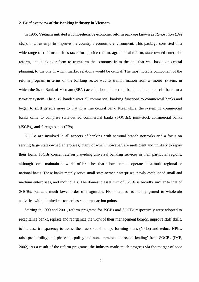
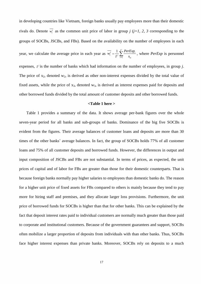
3.1. Graphical illustration
Consider a simple example of a bank (say k‘) producing one output, y, using one input, x. In
Figure 1, the bank‘s input-output levels are depicted by vector z, and its current operation is
technically inefficient as point A is off the frontier that defines the feasible technology set (the
shaded are is the feasible set of input-output combinations under the available technology). To be
technically efficient, the bank needs to simultaneously reduce input and increase output along the
directional vector given by g = (-gx gy)‘, by the movement from the current point, A, to point B
where vector AD (that is parallel to g) passes through the frontier. Thus, a natural measure of
technical inefficiency would be a ratio of the distance between A and B, |AB|, to the total distance
9
from O to A and then B, namely |OA|+|AB|. When point B‘ is located along the extension of z such
that |AB|=|AB‘|, the technical inefficiency score can be defined as |AB‘|/|OB‘|, and hence the
technical efficiency score as |OA|/|OB‘|.
<Figure 1 here>
The parallel lines passing through points A, B, C and D on vector AD are the price lines the
bank is facing, whose slope equals the input price, denoted wk‘
, divided by the output price, denoted
pk‘
. When the bank is allowed to change the input-output mix in any direction, the maximum profit
can then be achieved at a point where the price line is tangent to the feasible set, namely at point Q*.
Let C be the point where the price line that is tangent to the frontier crosses vector AD, and let π, πT,
and π* denote the actual profit at point A, the profit at the technically efficient point B and the
optimal profit achievable under the given price vector (wk‘
pk‘
)‘ at point Q* respectively. Then, the
ratio between the differences in the profits given by (πT−π)/(π
*−π), equals |AB|/|AC| since the heights
of the parallel price lines along the vertical axis represent profit levels normalised by the same
constant which is output price, pk‘
. It implies that |AB| is proportional to the additional profit the
bank can achieve to become technically efficient, and |AC| is proportional by the same proportion to
the additional profit the bank can achieve when it is allowed to change the input-output mix and
attain the maximum profit under the given prices. Furthermore, as |AC| equals |AB|+|BC|, |BC| is
proportional by the same proportion to (π*−π
T), which is the additional profit the bank can achieve
over the profit it makes at the technically efficient point when it changes input-output bundle and
becomes allocatively efficient on top of being technically efficient. So, analogous to the definition of
technical inefficiency, allocative inefficiency can be defined as |BC|/(|OA|+|AB|+|BC|), which is
equal to |B‘C‘|/|OC‘| where C‘ is located along the extension of z such that |AC|=|AC‘|. The
allocative efficiency index is then defined by |OB‘|/|OC‘|, and the profit efficiency index by
|OA|/|OC‘|, which is the product of technical efficiency and allocative efficiency. Note that profits
may be negative, but π* will be always at least as great as π
T which is in turn at least as great as π,
10
hence negative profits will not cause a trouble in the definitions of indices. When π equals π*,
technical efficiency, allocative efficiency and profit efficiency will be all one.
3.2. A new index approach
Consider a banking industry where banks produce M outputs using N inputs, that is, input vector
x NR and output vector y MR . Let z = (x‘ y‘)‘ MNR be the actual input output vector, g =
( gx‘ gy‘)‘ MNR be the directional vector, and p = ( w‘ p‘)‘ NR MR be the vector of
negative input prices and positive output prices.
We define the feasible set T ⊆ NR × MR under the available technology as
T = {(x,y): x can produce y} (1)
Then, the directional (technology) distance function is defined by (Luenberger, 1992; Chambers et
al., 1998):
* = D
(z;g,T) = max {β: (z + βg) T} (2)
where * is the solution to the conditional maximisation problem. Since z T, β
* is non-negative.
1 If
* equals zero, it implies that it is technically impossible to simultaneously contract inputs and
expand outputs from the current levels and hence the bank is technically efficient. When * is greater
than zero, on the other hand, it is implied that there is room for an increase in the profit by producing
more outputs using less inputs. The maximum simultaneous reductions in the inputs and increases in
the outputs that the bank can make along the directional vector are by *g, whose equivalence in
Figure 1 is AB. Thus the maximum profit achievable at the technically efficient point is given by
T = p∙(z +
*g) = p∙z +
*p∙g = +
* (3)
where is the actual profit and = p∙g = w‘gx + p‘gy which is strictly positive given that g is not a
null vector. Rearranging equation (3) for * yields
* = (
T )/ . (4)
1 See Lemma 2.1 of Chambers et al. (1998, p354).

11
Similarly, the maximum profit the bank can achieve when changes in input-output bundle are
allowed is calculated as
* = p∙(z + 1g) = p∙z + 1p∙g = + 1 (5)
where 1 is non-negative scalar value that makes the first equation in (5) hold. The new input-output
vector, (z + 1g), may not be feasible under T, but a 1 should exist to make the equation
algebraically true. Rearranging (5) for 1 gives
1 = (π* − π)/δ. (6)
In Figure 1, |AB| which represents technical inefficiency equals β* times the length of the
directional vector, i.e. β*|g|. This implies that |AC| equals λ1 times the length of the directional vector,
i.e. λ1|g|, and |BC| which represents allocative inefficiency equals λ1|g|− β*|g|. Comparing equations
(3) and (5) reveals that λ1 ≥ β* because π* ≥ π
T and δ > 0. Thus, λ1|g|− β
*|g| ≥ 0.
We are now ready to define our technical efficiency (TE), allocative efficiency (AE), and profit
efficiency (PE) scores as:
TE = 1 *|g|/(|z|+
*|g|) = |z|/(|z|+
*|g|), (7)
AE = 1 – (λ1|g|− β*|g|)/(|z|+λ1|g|) = (|z|+
*|g|)/(|z|+λ1|g|), and (8)
PE = |z|/(|z|+λ1|g|). (9)
Note that PE=TE×AE. The lengths of the vectors, |z| and |g|, are measured as Euclidean distances,
zz and gg , respectively.
As alluded at the beginning of this section when we used notations wk‘
and pk‘
for the input and
output prices faced by bank k‘, individual banks face different input and output prices. The
difference between output price and input price represents banking margin, and hence it may well
reflect bank‘s business skills as well as its reputation and credit rating. Thus, we next look at banks‘
such skills, namely, their efficiency in securing the most favourable input-output price ratios. In
Figure 1, the maximum profit a bank can achieve when price negotiation skills are allowed for is
denoted by πm
and the most favourable output price by pm
. The most favourable price line is tangent
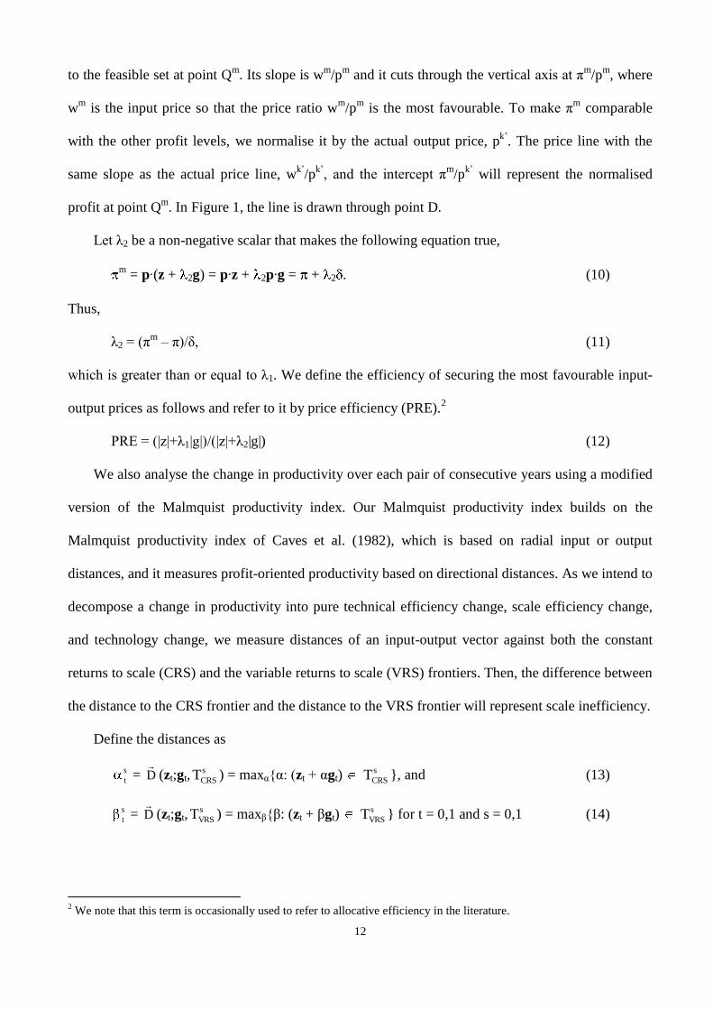
12
to the feasible set at point Qm
. Its slope is wm
/pm
and it cuts through the vertical axis at πm
/pm
, where
wm
is the input price so that the price ratio wm
/pm
is the most favourable. To make πm
comparable
with the other profit levels, we normalise it by the actual output price, pk‘
. The price line with the
same slope as the actual price line, wk‘
/pk‘
, and the intercept πm
/pk‘
will represent the normalised
profit at point Qm
. In Figure 1, the line is drawn through point D.
Let λ2 be a non-negative scalar that makes the following equation true,
m
= p∙(z + 2g) = p∙z + 2p∙g = + 2 . (10)
Thus,
λ2 = (πm
– π)/δ, (11)
which is greater than or equal to λ1. We define the efficiency of securing the most favourable input-
output prices as follows and refer to it by price efficiency (PRE).2
PRE = (|z|+λ1|g|)/(|z|+λ2|g|) (12)
We also analyse the change in productivity over each pair of consecutive years using a modified
version of the Malmquist productivity index. Our Malmquist productivity index builds on the
Malmquist productivity index of Caves et al. (1982), which is based on radial input or output
distances, and it measures profit-oriented productivity based on directional distances. As we intend to
decompose a change in productivity into pure technical efficiency change, scale efficiency change,
and technology change, we measure distances of an input-output vector against both the constant
returns to scale (CRS) and the variable returns to scale (VRS) frontiers. Then, the difference between
the distance to the CRS frontier and the distance to the VRS frontier will represent scale inefficiency.
Define the distances as
s
t = D
(zt;gt,s
CRST ) = maxα{α: (zt + αgt) s
CRST }, and (13)
s
t = D
(zt;gt,s
VRST ) = maxβ{β: (zt + βgt) s
VRST } for t = 0,1 and s = 0,1 (14)
2 We note that this term is occasionally used to refer to allocative efficiency in the literature.
13
where t and s are either base period (0) or comparison period (1), zt = (xt‘ yt‘)‘ is the input-output
vector in period t, gt is the directional vector in period t, s
CRST is the CRS feasible technology set in
period s, and s
VRST is the VRS feasible technology set in period s. Then, the Malmquist productivity
index between two periods is defined as the geometric mean of two productivity indices – one based
on period 0‘s and the other based on period 1‘s technology:
M0,1
=
2/1
0
1
1
1
0
0
1
0
)z(M
)z(M
)z(M
)z(M (15)
where Ms(zt) = |zt|/[|zt|+
s
t |gt|] , for t=0,1 and s=0,1. Note that each Ms(zt) can be decomposed into
1/[1+ s
t ] and [1+ s
t ]/[1+ s
t ], where s
t = s
t |gt|/|zt| and s
t = s
t |gt|/|zt|, representing technical
efficiency and scale efficiency of zt respectively. When these are substituted into (15), the profit-
oriented Malmquist productivity index can be rewritten as follows.
M0,1
=
2/1
1
0
1
0
1
1
1
1
0
0
0
0
0
1
0
1
)1/()1(
)1/()1(
)1/()1(
)1/()1(
)1/(1
)1/(10
0
1
1
2/1
1
0
0
0
1
1
0
1
)1/(1
)1/(1
)1/(1
)1/(1(16)
The terms in the three sets of brackets on the right-hand side of the equation are scale efficiency
change (SEFFCH), pure technical efficiency change (TEFFCH), and technological change
(TECHCH), respectively. The SEFFCH in the first set of brackets is the geometric mean of two scale
efficiency ratios, one based on period 0‘s and the other based on period 1‘s technology. The
TEFFCH in the second set of brackets measures how much closer (or farther) the input-output vector
has moved to the corresponding period‘s VRS technology frontier. The TECHCH in the last set of
brackets is the geometric mean of two measures of the shift in the frontier, one along the input-output
vector in period 0 and the other along the input-output vector in period 1. This definition of
productivity index is in a ratio form and thus is in line with the earlier definitions of efficiency
measures. It contrasts with the Luenberger productivity indicator defined in terms of differences by
Chambers et al. (1996).
14
Following Färe et al. (2004), the Data Envelopment Analysis (DEA) method is used to construct
frontiers defining technology sets and to measure distances to the frontiers. For the DEA models of
the present paper, we assume that the underlying technology is characterised by VRS. Further, to
account for the potential tradeoff between risk and profit, equity capital is included as a fixed input.
Other considerations include two important regulatory constraints faced by the banks operating in
Vietnam that the equity capital of a domestic bank should be at least a certain proportion of its total
risk-weighted asset (capital-adequacy constraint) and that the total amount of deposits by Vietnamese
nationals with a foreign bank cannot exceed a set multiple of its equity capital (deposit constraint).
We will estimate the models with and without the capital-adequacy and deposit constraints to analyse
the effects of those constraints.
Specifically, the maximal short-run unregulated profit that is attainable by a decision making
unit (DMU), k‘, facing input and output prices, wk‘
and pk‘
respectively, is estimated by solving the
following linear programming (LP) problem:
π* = maxy,x,v {p
k‘∙y – w
k‘∙x:
K
1k
k
mk yv ≥ ym m = 1, . . ., M
K
1k
k
nk xv ≤ xn n = 1, . . ., N
K
1k
k
kev ≤ ek‘
K
1k
kv = 1
x ≥ 0N, y ≥ 0M, and vk ≥ 0 for k = 1, . ., K} (17)
where K is the total number of DMUs, vk are the intensity variables, ym is the mth
element of the
output vector y, xn is the nth
element of variable input vector x, and e is equity capital.
The maximal short-run regulated profit for the same DMU is computed by adding the following two
additional constraints:
(i) capital-adequacy constraint: R
1r
'k
rr
'k A/e ≥ μe if k‘ is not a foreign bank; and
(ii) deposit constraint: x3VN
/ek‘
≤ μd if k‘ is a foreign bank, (18)

15
where Ar and ωr are risk-assigned assets and their risk weights respectively, x3VN
is the total deposit
with bank k‘ by Vietnamese nationals, and μe and μd are constants set by the regulator.
The directional distance to the VRS frontier of the input-output vector of DMU k‘ is measured
by
* = max { :
K
1k
k
mk yv ≥ ym
'k
m gy m = 1, . . ., M
K
1k
k
nk xv ≤ xn
'k
n gx n = 1, . . ., N
K
1k
k
kev ≤ ek‘
K
1k
kv = 1,
β ≥ 0 and vk ≥ 0 for k = 1, . ., K} (19)
where gxn and gym are the nth
and the mth
elements of gx and gy respectively. Distances to the CRS
frontier can be measured when the VRS constraint, K
1k
kv = 1, is excluded.
The Malmquist productivity index defined by (16) requires computation of the distance of an
input-output vector in one period against the frontier in the other period, like the computation of
D
(zt;gt,sT ) where t ≠ s. In such cases, some efficient DMU‘s input-output vector becomes infeasible
under the other period‘s technology. The LP problems in those cases are modified as follows.
* = max {− :
K
1k
k
mk yv ≥ ym
'k
m gy m = 1, . . ., M
K
1k
k
nk xv ≤ xn
'k
n gx n = 1, . . ., N
K
1k
k
kev ≤ ek‘
K
1k
kv = 1,
β ≥ 0 and vk ≥ 0 for k = 1, . ., K} (20)
To measure distances against a CRS frontier, the VRS constraint, K
1k
kv = 1, is excluded. Note that
the solution to the above LP problem for an infeasible DMU in the original LP problem, (19), is
16
negative, and hence the technical efficiency measure |z|/(|z|+β|g|) is greater than one, implying that
the DMU is ―super efficient‖ under the reference technology.3
4. Data
We adopt the intermediation approach and define the outputs as customer loans (y1), other
earning assets (y2), and the actual value of off-balance-sheet items (y3), and the inputs as full-time
equivalent number of employees (x1), fixed assets (x2), customer deposits, and other borrowed funds
(x3), plus equity capital (e) as a fixed input. All input and output values are deflated with the
consumer price index (CPI).4
The price of y1, denoted p1, is derived as the amount of interest income from customer loans
divided by the amount of customer loans. The price of y2, denoted p2, is derived similarly as the
amount of other interest and investment income divided by the amount of other earning assets.
Necessary information to derive the price for off-balance-sheet items (y3), denoted p3, is not
available for all banks. Hence, we compute p3 as non-interest income divided by the value of off-
balance-sheet items for the banks where separate series are available. Then, the average of those p3
values in each year is used as the price of y3 for all banks in that year assuming that p3 is identical for
all banks in each year. Similarly, as the number of full-time equivalent employees was not available
for all individual banks in Vietnam, we assume that the unit price of labor (w1) is the same for all
banks in the same ownership category, but varies from year to year. This assumption is based on the
fact that banks in the same ownership category normally offer quite similar salary level. Furthermore,
3 It is noted that even the modified LP problem may not have a solution in some extreme cases. The modified problem
will not have a solution when the reverse extension of the directional vector, such as vector AD in Picture 1, passes
through the hyperplane formed by the input axes at a point outside the feasible set. For example, when the actual input-
output vector is used as the directional vector there will be no solution to the modified LP problem if the minimal level of
any input among all the DMUs in the technology set is greater than two times the level of the same input used by the
DMU in question. The data set used in the following section does not have such cases and all distances can be found by
either the original problem or the modified problem. See Ray (2007) for more discussions.
4 It should be noted that the correlation coefficient between CPI and GDP deflator in Vietnam during the studied period
was almost equal to one. Thus, the use of either variable to deflate the nominal values of data should result in no
significant differences in the results
17
in developing countries like Vietnam, foreign banks usually pay employees more than their domestic
rivals do. Denote 1
jw as the common unit price of labor in group j (j=1, 2, 3 corresponding to the
groups of SOCBs, JSCBs, and FBs). Based on the availability on the number of employees in each
year, we calculate the average price in each year as 1
1 1
1jI
j i
ji i
PerExpw
xI, where PerExp is personnel
expenses, jI is the number of banks which had information on the number of employees, in group j.
The price of x2, denoted w2, is derived as other non-interest expenses divided by the total value of
fixed assets, while the price of x3, denoted w3, is derived as interest expenses paid for deposits and
other borrowed funds divided by the total amount of customer deposits and other borrowed funds.
<Table 1 here >
Table 1 provides a summary of the data. It shows average per-bank figures over the whole
seven-year period for all banks and sub-groups of banks. Dominance of the big five SOCBs is
evident from the figures. Their average balances of customer loans and deposits are more than 30
times of the other banks‘ average balances. In fact, the group of SOCBs holds 77% of all customer
loans and 75% of all customer deposits and borrowed funds. However, the differences in output and
input composition of JSCBs and FBs are not substantial. In terms of prices, as expected, the unit
prices of capital and of labor for FBs are greater than those for their domestic counterparts. That is
because foreign banks normally pay higher salaries to employees than domestic banks do. The reason
for a higher unit price of fixed assets for FBs compared to others is mainly because they tend to pay
more for hiring staff and premises, and they allocate larger loss provisions. Furthermore, the unit
price of borrowed funds for SOCBs is higher than that for other banks. This can be explained by the
fact that deposit interest rates paid to individual customers are normally much greater than those paid
to corporate and institutional customers. Because of the government guarantees and support, SOCBs
often mobilize a larger proportion of deposits from individuals with than other banks. Thus, SOCBs
face higher interest expenses than private banks. Moreover, SOCBs rely on deposits to a much
18
greater extent than the other bank types, hence the impact of such higher cost sources of funds is all
the greater.
It is generally accepted that banking is one of the most regulated industries in any country.
Among regulations, prudential regulations are particularly crucial in transitional economies. Lessons
from the Asian financial crisis demonstrated that inadequate prudential restrictions could lead finally
to monetary and financial crises (Mishkin, 1999). Some prudential regulations can have positive
effects on the level of efficiency because they induce banks‘ management to care more about risk-
taking and allocating resources more efficiently. For example, capital-adequacy requirements reduce
banks‘ overexposure to risky assets, and bank managers therefore need to adjust their output
portfolios, leading to better allocative efficiency. This paper is therefore concerned about the effect
of the minimum capital-asset requirement on the profit performance of banks in Vietnam.
Additionally, one of the biggest restrictions on foreign bank branches operating in Vietnam is the
limitation imposed on deposit taking. Hence, the paper is interested in how this limitation affects the
profit performance of foreign bank branches.
The capital-adequacy regulation is applied to all banks except foreign banks, whereas the deposit
regulation is applied only to foreign banks. The capital-adequacy regulation currently adopted by the
Vietnamese regulator is the minimum ratio of equity capital to risk weighted assets. A bank is
regarded as adequately capitalised if the ratio is at least 8%, which is equivalent to μe in (18). Total
risk-weighted assets in (18) is computed as
Risk-weighted assets = ω1y1 + ω2y2 + ω3y3c + ω4x2 + ω5OA (21)
where ωi are risk weights, c is the conversion ratio for off-balance-sheet items, and OA is other
assets which is explained below. Risk weights for the variables defined in the present paper are
estimated as a weighted average of the risk weights for the sub-assets included in each variable. The
risk weight for Customer Loans (y1) is 55% reflecting various degrees of risk associated with loans
with different types of securities, ranging from 0% for loans secured by deposits with the bank itself
to 100% for loans secured by a third-party property. Other Earning Assets (y2) carries a risk weight
19
of 25% representing balances with other financial institutions and securities. Off-balance-sheet Items
(y3) is converted to a value equivalent to balance-sheet items by multiplying by the conversion ratio
of 0.5 before the risk weight 50% is applied. Fixed Assets (x2) carries a risk weight of 100%. There
are other assets (OA) that are not included in any of the output variables or Fixed Assets, while they
should be included in the measure of risk-weighted assets for capital-adequacy. Those assets include
balance with the central bank, cash and equivalent, and non-performing loans. OA carries a risk
weight of 60%.
Note that the capital-adequacy constraint is imposed in the profit-maximisation problem, (17), as
ω1y1 + ω2y2 + ω3y3c + ω4x2 ≤ (ek‘
/μe) – ω5OAk‘
(22)
while it is imposed for the directional distance function, (19), as
β(ω1gy1 + ω2gy2 + ω3gy3c − ω4gx2) ≤
(ek‘
/μe) – (ω1y1k‘
+ ω2y2k‘
+ ω3y3k‘
c + ω4x2k‘
+ ω5OAk‘
). (23)
Also note that when the bank in question, k‘, violates the capital-adequacy regulation the LP problem
for the directional distance usually does not have a feasible set, but the LP problem for maximum
profit may have one. The former is the case because the right-hand side of (23) becomes negative
while the term in parentheses on the left-hand side is usually positive. On the other hand, the
violation does not automatically make the profit-maximisation problem infeasible because an
optimum input-output vector can still be found such that the constraint (22) is satisfied.
Up to December 2001, the maximum amount of deposits any foreign bank can take from
Vietnamese nationals (natural or legal persons) had been 25% of equity capital. However, the
bilateral trade agreements with U.S. and European countries have led to a gradual relaxation of this
limit to 700% from legal persons plus 650% from natural persons for U.S. banks and 400% from
legal persons plus 350% from natural persons for European banks by the end of 2006. Other foreign
banks‘ limit has also been relaxed to 50% from October 2003. For each year, the limits applied to
different groups of foreign banks are computed as a weighted average of limits for legal and natural

20
persons with the weights reflecting the number of days different limits have been valid for. Table 2
shows the limits applied to the deposit constraint for the three groups of foreign banks in each year.
<Table 2 here>
The deposit constraint is imposed as
x3 ≤ 'k,VN'k'k
d r/e (24)
where 'k
d is the deposit limit applied to bank k‘, 'k,VNr is deposit by Vietnamese nationals with bank
k‘ divided by total deposits with the bank, x3VN,k‘
/x3k‘
, which is assumed to be fixed during the
optimisation process. Note that the above constraint is not applicable to the estimation of distance
because contracting x3 by βgx3 would make the left-hand side term of the inequality in (24) even
smaller than x3. So, the deposit constraint is imposed only in the profit maximisation problem.
Finally, the directional vector, g = (−gx‘ gy‘)‘, is defined as the actual input-output vector, (−x‘
y‘)‘. Although there are other alternatives, such as a unit vector or average of inputs and outputs over
banks, this approach has an important advantage over others. That is, only it enables valid
interpretation of allocative efficiency measures. When the directional vector is defined as the actual
input-output vector, the TE, AE, PE, and PRE scores defined in the previous section are simplified as
1/(1+β*), (1+β
*)/(1+λ1), 1/(1+λ1), and (1+λ1)/(1+λ2) respectively. The components of the Malmquist
productivity index, (16), are also similarly simplified.
5. Empirical findings
5.1. Estimates of efficiency
Directional distance and maximum profit under a given price vector have been computed for
each of the 56 banks in each year by solving the LP problems defined by (17) and (19) respectively,
with and without the capital-adequacy and the deposit constraints.5 In each year, the feasible
technology set is defined as the polyhedron enveloping the input-output vectors observed in the
5 The econometrics software program Shazam V10 (Whistler et al., 2004) has been used for the computation. A few
instances of ―computer cycling‖ were encountered during the computation, but they could be easily overcome by
changing the units of measurement. See Gass and Vinjamuri (2004) for more details on computer cycling in LP
problems.
21
current and the years preceding it. Feasible technology sets based on this approach, which is not new
in the literature,6 would more closely resemble the reality where a once-used technology is generally
available in the following years unless there exist restrictions preventing it.
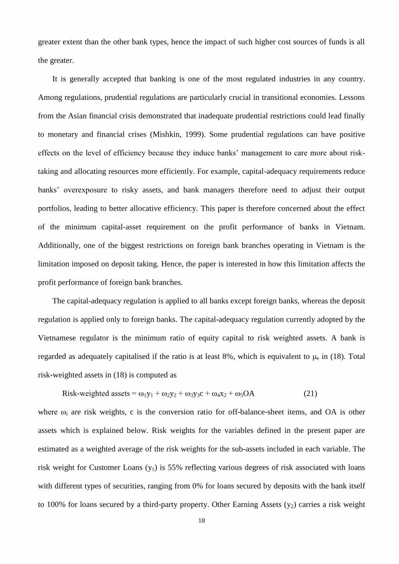
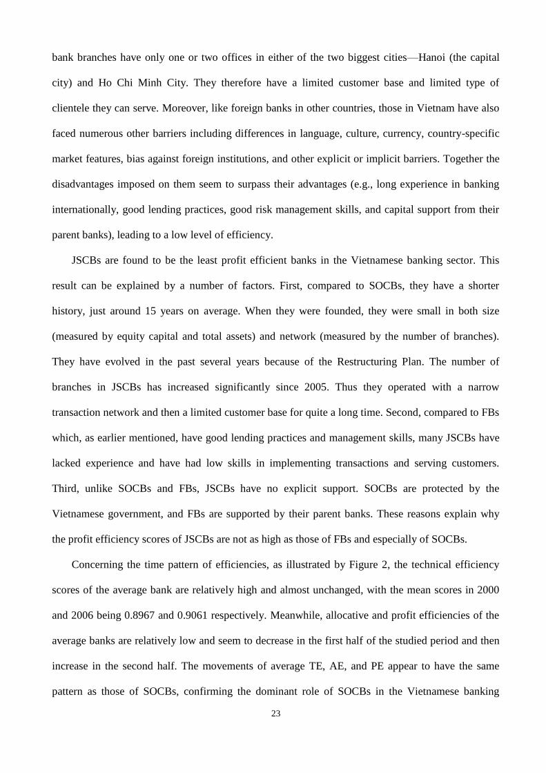
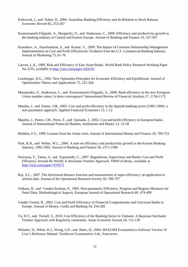
The graphs in Figure 2 show geometric average technical efficiency (TE), allocative efficiency
(AE), profit efficiency (PE), and price efficiency (PRE) scores for all and subgroups of banks in each
year, with the capital-adequacy constraint and the deposit constraint imposed on domestic banks and
foreign banks respectively. There are 19 cases out of the 273 (39 domestic banks times 7 years) LP
problems for directional distance where the bank in question violates the capital-adequacy regulation
with the ratio of equity capital to risk-weighted assets falling below 8%. Of the 19 violations, 13
have been committed by SOBs, implying that the penalty fines imposed by the regulator have not
been heavy enough to deter big banks from violating the regulation. Directional distances for those
19 cases have been set to zero, implying that the banks involved are technically efficient.7 Further, in
4 cases out of those 19 cases, actual profit is higher than the maximum profit attainable under given
prices. The banks in those cases are assumed to be allocatively efficient.
<Figure 2 here>
Average TE scores lie within a relatively narrow range of 0.84 and 1.0, while the AE scores
range between 0.33 and 0.88, implying that the main source of the difference in profit efficiency is
the difference in allocative efficiency. The low level of allocative efficiency in general might arise
because banks produce too much of one type of loan and too little of another. This likely happens to
domestic banks because they normally make a poor assessment of credit risk and do not utilize the
benefit of diversification. Meanwhile, foreign banks, even though they possess better skills of risk
assessment and management, focus too much on wholesale banking and ignore the retail banking
market, and thus do not diversify their loan portfolios. Furthermore, domestic banks appear to
employ too much labor relative to capital, leading to increased non-wage expenses such as capital
6 See, for example, Park and Weber (2006), and Tulkens and Vanden Eeckaut (1995).
7 In fact, the directional distances for those cases are zero except only for four cases when the capital-adequacy constraint
is excluded. Even for those four cases, the maximum value is only 0.06.

22
equipment and working space. These factors cause the actual relative prices of banks to differ from
the shadow relative prices at which banks can maximize profits.
The big five state-owned banks not only enjoy a lion‘s share of both credit and lending markets
(Table 1), but they make their huge profits most efficiently, both technically and allocatively. This
may be due to various factors. First, SOCBs are owned by the state, and are thus the first banking
choice for state-owned enterprises, especially large and pivotal enterprises (e.g., gas and petroleum,
electricity, export and import, and coal enterprises). SOCBs are also protected and guaranteed by the
government, so that they have a good reputation (for safety at least) with domestic depositors. These
advantages bring SOCBs a large market share in terms of deposits and lending, then market power in
the setting of prices, especially prices of banking outputs. Second, SOCBs are larger banks in terms
of total assets. It is found in the literature that larger banks are more efficient than smaller banks
(Laeven, 1999; Berger et al., 2009). Third, SOCBs have a relatively long history and broader market
base via their nationwide branching networks, factors which in turn bring them various benefits. For
instance, increased savings from the wide network increase the amount of funds available for lending
and investment. In addition, the presence of a wide range of branches makes it easier for individuals
and small businesses to access credit and other financial services (Gottschang, 2001). However, even
though they are the most profit efficient in the Vietnamese banking sector, SOCBs still operate
below the profit frontier of the best practice banks. The reason for the deficiency is the lack of a
strong profit orientation in the SOCBs at two levels. At the national level, the SBV remains heavily
involved in the day-to-day management of SOCBs. The SBV Governor is responsible for the
appointment of Advisory Boards, top management positions and the Chairperson at SOCBs. At the
local level, the branches of SOCBs come under the close management of the SBV‘s branches in all
provinces.
The main reason for low profit efficiency scores for foreign banks is that they have been
restricted by a number of regulations. One of the most restrictive is that they have not been permitted
to open transaction points or offices outside their current branch offices. Consequently, most foreign
23
bank branches have only one or two offices in either of the two biggest cities—Hanoi (the capital
city) and Ho Chi Minh City. They therefore have a limited customer base and limited type of
clientele they can serve. Moreover, like foreign banks in other countries, those in Vietnam have also
faced numerous other barriers including differences in language, culture, currency, country-specific
market features, bias against foreign institutions, and other explicit or implicit barriers. Together the
disadvantages imposed on them seem to surpass their advantages (e.g., long experience in banking
internationally, good lending practices, good risk management skills, and capital support from their
parent banks), leading to a low level of efficiency.
JSCBs are found to be the least profit efficient banks in the Vietnamese banking sector. This
result can be explained by a number of factors. First, compared to SOCBs, they have a shorter
history, just around 15 years on average. When they were founded, they were small in both size
(measured by equity capital and total assets) and network (measured by the number of branches).
They have evolved in the past several years because of the Restructuring Plan. The number of
branches in JSCBs has increased significantly since 2005. Thus they operated with a narrow
transaction network and then a limited customer base for quite a long time. Second, compared to FBs
which, as earlier mentioned, have good lending practices and management skills, many JSCBs have
lacked experience and have had low skills in implementing transactions and serving customers.
Third, unlike SOCBs and FBs, JSCBs have no explicit support. SOCBs are protected by the
Vietnamese government, and FBs are supported by their parent banks. These reasons explain why
the profit efficiency scores of JSCBs are not as high as those of FBs and especially of SOCBs.
Concerning the time pattern of efficiencies, as illustrated by Figure 2, the technical efficiency
scores of the average bank are relatively high and almost unchanged, with the mean scores in 2000
and 2006 being 0.8967 and 0.9061 respectively. Meanwhile, allocative and profit efficiencies of the
average banks are relatively low and seem to decrease in the first half of the studied period and then
increase in the second half. The movements of average TE, AE, and PE appear to have the same
pattern as those of SOCBs, confirming the dominant role of SOCBs in the Vietnamese banking

24
sector. Moreover, allocative and profit efficiencies (for all banks as well as each category of banks)
appear to follow the same pattern, suggesting that allocative efficiency dominates technical
efficiency in shaping profit efficiency.
With regard to the type of ownership, the profit efficiency of JSCBs decreases continuously over
the period analysed, from the peak of 0.4612 in 2000 to the trough of 0.3509 in 2006. This finding
indicates that JSCBs move further and further away from the optimal bundle of inputs and outputs at
which profit can be maximized, and that the restructuring plan, which started in 1999, did not have a
positive effect on the performance of these banks in optimizing their input-output mix. This is
understandable in the sense that the restructuring program focused on organizational issues rather
than operational issues. It might take banks a few more years to adjust, adopt, get used to, and
operate smoothly under the new structure. The reduction in profit efficiency for JSCBs could be
attributed to their failure to manage their diverse activities (e.g., offering a wider range of products,
investing in technology, and enlarging branching network), hence spending more and earning less
(the increase in revenues being not as great as the increase in costs), leading to lower profitability.
In contrast, the profit efficiency of FBs evidenced a downward trend during the first half of the
sample period and then an upward trend in the second half (2003–2006). This evolution brought an
increase of 3% in profit efficiency for FBs across the 7-year period. The increase in profit efficiency
of FBs in the second half of the estimation period might be consistent with the view that when they
experience less regulatory control, engage in varied activities, and diversify products and services,
FBs manage to translate these factors into a higher level of profit efficiency.
For SOCBs, a major improvement in profit efficiency (of about 13%) occurs between 2000 and
2001, and the level then remains stable for 2002. In a similar pattern to the FBs, the profit efficiency
scores of SOCBs also reach their lowest in 2003 before tending upwards toward the end of the period.
Overall, SOCBs achieve an improvement in profit efficiency of nearly 20%. This significant
outcome could be considered a positive effect of the restructuring programs carried out on these
banks since 2001. The low level of profit efficiency in 2003 for SOCBs could be explained by the
25
fact that in this year, facing the rapid pace of credit growth (which likely led to a high ratio of non-
performing loans), SOCBs were more cautious in granting loans, thus reducing pressure on
mobilizing funds, and then marginal interest rates tended to decrease slightly, leading to lower
profitability. Examining the data set, the study observes that SOCBs faced the lowest marginal rate
(lending interest rate minus deposit interest rate) over the 7-year period in 2003, leading to a low rate
of profit growth, and then the lowest profit efficiency level.
As mentioned in Section 3, we also calculated price efficiency (PRE) scores to compare banks‘
abilities to secure the most profitable price ratios. In each year, each bank‘s profit-maximisation
problem, (17), has been solved with each of the actual 56 price vectors faced by all banks in that year.
Then, the maximum profit achievable among the 56 price vectors is regarded as πm
for the bank in
question in the corresponding year. Once λ2 is obtained, the price efficiency score is computed using
(12). Panel D of Figure 2 shows PRE scores. The full sample mean price efficiency is very low, just
around 0.17, implying that the observed input and output price level of the average bank in Vietnam
is substantially far behind the most favorable price level. Furthermore, the price efficiency level of
SOCBs is found to be much higher than that of JSCBs and FBs. This implies that private banks may
suffer higher costs in providing the same financial services as state-owned banks, or gain lower
revenues from providing the same quality and variety of services. This result suggests the existence
of a market power advantage for SOCBs in the setting of prices, even in the context of increased
competitive pressure. This could be reflected by differences in business between foreign banks and
domestic banks. Most of the foreign banks have focused on wholesale banking whereas domestic
banks have developed retail banking. Importantly, over the 7-year period, the price efficiency of all
groups increased by around 10%, suggesting that there has been an improvement in banks‘
credibility in the setting of prices.
The efficiency scores estimated without imposing the capital-adequacy and deposit constraints
are not separately tabulated to save space. Imposing the capital-adequacy constraint does not have
effect on the technical efficiency of domestic banks in most cases, and even for the few cases where

26
that has effect the largest difference is only 0.008. This implies that in most cases the directional
vector faces a facet of the technical frontier other than the one that is formed by the capital-adequacy
constraint. Imposing the capital-adequacy constraint causes some changes in the allocative efficiency
scores of domestic banks, with the mean absolute change being 0.025.8
The effects of the two constraints on allocative efficiency and profit efficiency are statistically
insignificant. The Kolmogorov-Smirnov (KS) statistic for the null hypothesis that the AE scores for
domestic banks with and without the capital-adequacy constraint are from the same distribution is
0.033 with a modified p-value of 0.998. Consequently, the effect of the constraint on profit efficiency
is also insignificant with the KS statistic 0.037 and its modified p-value 0.991. The KS statistics on
the deposit constraint are 0.126 and 0.118 for AE and PE respectively. Their modified p-values are
0.251 and 0.327, respectively, and hence relatively more significant than the statistics for the capital-
adequacy constraint. However, the null hypothesis still cannot be rejected at a usual level of
significance.
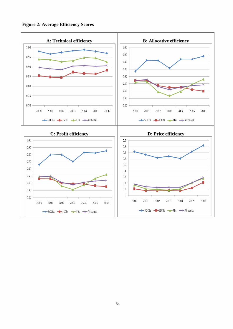
5.2. Estimates of productivity
The Malmquist productivity index defined by (16) has been computed for each bank in each year.
In computing the directional distances, both the capital-adequacy and deposit constraints are
excluded in constructing the frontiers. The reason is because such constraints would lead to biased
measures of scale efficiency for those cases where the directional vector cuts through the hyperplane
formed by the regulatory constraints. In such cases, scale inefficiency would be represented by the
distance to the constant-returns-to-scale (CRS) frontier from the frontier formed by the regulatory
constraint instead of the variable-returns-to-scale (VRS) frontier formed by the input-output
constraints. The productivity change (PROD) is decomposed into technical efficiency change
(TEFFCH), technological change (TECHCH), and scale efficiency change (SEFFCH). The over
mean estimates for these changes are reported in Table 3.
<Table 3 here>
8 Note that imposing an additional constraint cannot decrease TE but it may decrease AE.
27
Overall, the banking industry in Vietnam experiences modest productivity progress with an
average rate of 1.61% per annum. The main contributor to this growth is technological progress of
3% per year. Meanwhile, improvement in technical efficiency is tiny, just 0.16% on average, but
deterioration in scale efficiency is about 1.5% per year. Technological progress is large enough to
offset a decline in scale efficiency, leading to a moderate improvement in productivity.
At the bank category level, the results indicate that foreign banks have a higher rate of
productivity growth than the two groups of domestic banks. The driver for their achievement is an
improvement in technology, of about 4.3% per annum. Besides, they experience a mild contraction
in scale efficiency (−0.57%) and an insubstantial decrease in technical efficiency (−0.26%). The
plausible explanation for the high growth rate of productivity in foreign banks lies in their business
model. Unlike domestic banks, they focus on corporate and wholesale banking rather than retail
banking. Thus, they can adjust their production plans and operational scale better and more quickly
than others when facing changes in the banking environment. The other likely explanation is that
most foreign banks have more advanced technology platforms than SOCBs and especially JSCBs.
Clearly, they have been the leaders in the introduction of credit cards, debit cards, ATMs, factoring,
forfeiting, and other modern financial services. With these advantages, the penetration of foreign
banks into the Vietnamese market has promoted productivity gains of the whole banking system.
In contrast to FBs, JSCBs undergo a tiny rate of productivity growth, just 0.56% on average. This
growth is made up of gentle rates of technological progress and technical efficiency improvement
(0.99% and 0.5% respectively), which are just sufficient to trade off a decrease in scale efficiency of
0.93% each year. Similarly, SOCBs also experience poor productivity growth, 0.53% each year on
average. However, the driver to this growth is relatively different from that of JSCBs. SOCBs enjoy
impressive technological progress (10.1% each year on average), but also suffer from a large
contraction in scale efficiency (8.5% annually).
The main reason for the low rate of productivity growth in JSCBs is their primitive technology
applications. Even though it appears that technology has been upgraded recently in some large

28
JSCBs, the common technology application at JSCBs is the application of core-banking software
which is used to computerize information and payment transactions. SOCBs have a much more
substantial technology infrastructure than JSCBs because they are subsidized by the government to
develop ATM networks, non-physical banking (i.e. internet banking, phone banking, and SMS
banking), and international card products. However, SOCBs exhibit only modest productivity growth.
The possible explanation is that they operate far beyond the optimal scale size, leading to a large
decrease in scale efficiency from year to year.
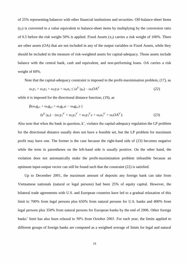
<Figure 3 here>
Figure 3 provides a picture of the evolution of productivity change and its components over
2000–2006 for the whole industry and for each bank category. The average bank in the sample seems
to enjoy productivity gains during 2000–2005 at different rates from one year to another (with the
highest rate of 4% in 2004), then experiences productivity loss in 2006. The loss in 2006 is primarily
caused by a decrease in scale efficiency, which is large enough to negate technological advancement
and technical efficiency growth.
At the category level, it seems that the TECHCH and SEFFCH of SOCBs develop in opposite
directions throughout 2000–2006, whereas the TEFFCH is quite stable and almost unchanged.
SOCBs achieve a very high rate of technological progress in 2001 compared to 2000 (nearly 20%),
then display much lower rates of technical improvement during 2002–2005 (at the average of around
6%) before regaining the high rate in 2006 (around 17%). Meanwhile, they suffer a large decrease in
scale efficiency between 2000 and 2001 (around −11%), then achieve lower rates of scale efficiency
loss before showing the largest rate of deterioration in scale efficiency in 2006 compared to 2005
(nearly −15%). These two factors almost offset each other, leading to moderate changes in
productivity of SOCBs from year to year and poor productivity growth on average over the 7 years
under study.
At JSCBs, it also appears that TECHCH and SEFFCH move in opposite directions to each other
almost every year (except for 2005), but their TEFFCH fluctuates more than that of SOCBs. As a

29
result, JSCBs undergo productivity expansion until 2004, and then show productivity contraction in
the last two years. The explanation for this productivity deterioration is that in 2004 JSCBs began to
enlarge their operations by opening more new branches. Correspondingly, their inputs, such as the
number of staff and fixed assets, increase dramatically. Meanwhile, no equivalent increase in outputs
occurs, at least in the short term. This causes a decrease in actual average productivity, and then a
lower rate of productivity growth.
In contrast, at FBs, TEFFCH, TECHCH, and SEFFCH seem to follow the same trend in most
years. Of these, TECHCH is the most volatile factor, followed equally by the other two factors. That
explains why the productivity change of these banks appears to fluctuate more than that of domestic
banks.
6. Conclusions
We have introduced a new approach to constructing technical efficiency, allocative efficiency,
and profit efficiency indices using directional distances. Unlike the available indicator approaches
that are based on differences, the new indices are based on ratios between distances, hence making
interpretations more sensible. We have also decomposed the Malmquist productivity index into scale
efficiency change, pure technical efficiency change, and technological change in a way that is fully
consistent with the new ratio-type efficiency indices. In doing so, we have explicitly shown how to
handle infeasible linear-programming problems when the directional distance of an input-out vector
is measured against the technology frontier in another period.
The new methods have been then applied to an analysis of the Vietnamese banking sector. The
findings show that the average bank operated quite far below the frontier of the best-practice bank.
The main source of this low profit efficiency was allocative inefficiency rather than technical
inefficiency, suggesting that banks were particularly poor at choosing input and output combinations
to maximize profits. Price efficiency was found to be significantly low, indicating that the actual
price vectors of banks in Vietnam were very different from the most favorable price vector. The
implication is that the majority of banks in Vietnam have more room to negotiate borrowing and
30
lending interest rates more favorably to maximize their profit. Moreover, the price efficiency scores
of SOCBs were much higher than those of JSCBs and FBs. This suggests that market power might
exist in pricing bank products in Vietnam, and that SOCBs have the power to set price ratios in such
a way that their profitability is maximized, whereas other banks cannot do so. We further found that
SOCBs were more profit efficient than FBs and domestic private banks. This result can be explained
by the fact that SOCBs benefit from being guaranteed and supported by the government, and having
nationwide branch networks as well as a huge customer base. The result can also be supported by the
preceding argument that market power might exist for state-owned banks in pricing bank outputs.
Furthermore, the effects of the two regulatory constraints are found to be insignificant both in size
and statistical sense
Regarding productivity analysis, the Vietnamese banking industry experienced modest
productivity growth, which is mainly due to technological progress, and to some degree technical
efficiency change, whereas scale efficiency change contributed adversely to productivity growth. The
most successful group, in terms of productivity improvement, appears to be the group of foreign
banks. Their technical efficiency and the growth rate of technology are better than any other groups
except SOCBs, resulting in the highest improvement in overall productivity, including SOCBs, over
the sample period.
Policy implications of the findings are that i) Policies that would result in the expansion of the
size of SOCBs would lead to significant decrease in their productivity due to deteriorating scale
efficiency; ii) To promote productivity growth, domestic banks need to manage their scale of
operation effectively and further upgrade their information technology platform, whereas foreign
banks need to enlarge their scale size through opening new offices and transaction points; and (iii)
The capital-adequacy constraint does not impose significant restriction on efficiency, and hence it
should be more strictly applied to enhance the stability of the financial system.

31
References
Ariff, M., and Can, L., 2008. Cost and profit efficiency of Chinese banks: A non-parametric analysis. China
Economic Review 19, 260-273
Berger, A.N., Hancock, D., and Humphrey, D.B., 1993. Bank efficiency derived from the profit function.
Journal of Banking and Finance 17, 317-347
Berger, A.N., Hasan, I., and Zhou, M., 2009. Bank ownership and efficiency in China: What will happen in
the world's largest nation. Journal of Banking and Finance 33, 113-130
Berger, A.N., and Mester, L.J., 1999. What Explains the Dramatic Changes in Cost and Profit Performance of
the U.S. Banking Industry? SSRN eLibrary, available at http://ssrn.com/abstract=155611
Briec, W., and Kerstens, K., 2009. The Luenberger productivity indicator: An economic specification leading
to infeasibilities. Economic Modelling 26, 597-600
Caves, D.W., Christensen, L.R., and Diewert, W.E., 1982. The Economic Theory of Index Numbers and the
Measurement of Input, Output, and Productivity. Econometrica 50, 1393-1414
Chambers, R.G., Chung, Y., and Färe, R., 1998. Profit, Directional Distance Functions, and Nerlovian
Efficiency. Journal of Optimization Theory and Applications 98, 351-364
Chambers, R.G., Färe, R., and Grosskopf, S., 1996. Productivity Growth in APEC Countries. Pacific
Economic Review 1, 181-190
DeYoung, R., and Hasan, I., 1998. The performance of de novo commercial banks: A profit efficiency
approach. Journal of Banking and Finance 22, 565-587
Färe, R., Grosskopf, S., and Weber, W.L., 2004. The effect of risk-based capital requirements on profit
efficiency in banking. Applied Economics 36, 1731-1743
Gass, S.I., and Vinjamuri, S., 2004. Cycling in Linear Programming Problems. Computers and Operations
Research 31, 303-311
Gottschang, T.R., 2001. The Asian Financial Crisis and Banking Reform in China and Vietnam. Department
of Economics Research Series Working Paper No.02-02, College of the Holy Cross
Hung, N.V., 2007. Measuring Efficiency of Vietnamese Commercial Banks: An Application of Data
Envelopment Analysis. In: Minh NK and Long GT (eds.) Technical Efficiency and Productivity Growth in
Vietnam. Publishing House of Social Labour, Hanoi, Vietnam.
IMF, 2002. Vietnam: 2001 Article IV Consultation. IMF Country Report No.02/4, International Monetary
Fund, Washington, D.C
IMF, 2003. Vietnam: Selected issues. IMF Country Report No.03/381, International Monetary Fund,
Washington, D.C
Kasman, A., and Yildirim, C., 2006. Cost and profit efficiencies in transition banking: the case of new EU
members. Applied Economics 38, 1079-1090
32
Kirkwood, J., and Nahm, D., 2006. Australian Banking Efficiency and Its Relation to Stock Returns.
Economic Record 82, 253-267
Koutsomanoli-Filippaki, A., Margaritis, D., and Staikouras, C., 2009. Efficiency and productivity growth in
the banking industry of Central and Eastern Europe. Journal of Banking and Finance 33, 557-567
Krasnikov, A., Jayachandran, S., and Kumar, V., 2009. The Impact of Customer Relationship Management
Implementation on Cost and Profit Efficiencies: Evidence from the U.S. Commercial Banking Industry.
Journal of Marketing 73, 61-76
Laeven, L.A., 1999. Risk and Efficiency in East Asian Banks. World Bank Policy Research Working Paper
No.2255, available at http://ssrn.com/paper=629192
Luenberger, D.G., 1992. New Optimality Principles for Economic Efficiency and Equilibrium. Journal of
Optimization Theory and Applications 75, 221-264
Mamatzakis, E., Staikouras, C., and Koutsomanoli-Filippaki, A., 2008. Bank efficiency in the new European
Union member states: Is there convergence? International Review of Financial Analysis 17, 1156-1172
Maudos, J., and Pastor, J.M., 2003. Cost and profit efficiency in the Spanish banking sector (1985-1996): a
non-parametric approach. Applied Financial Economics 13, 1-12
Maudos, J., Pastor, J.M., Perez, F., and Quesada, J., 2002. Cost and profit efficiency in European banks.
Journal of International Financial Markets, Institutions and Money 12, 33-58
Mishkin, F.S., 1999. Lessons from the Asian crisis. Journal of International Money and Finance 18, 709-723
Park, K.H., and Weber, W.L., 2006. A note on efficiency and productivity growth in the Korean Banking
Industry, 1992-2002. Journal of Banking and Finance 30, 2371-2386
Pasiouras, F., Tanna, S., and Zopounidis, C., 2007. Regulations, Supervision and Banks' Cost and Profit
Efficiency Around the World: A Stochastic Frontier Approach. SSRN eLibrary, available at
http://ssrn.com/paper=970373
Ray, S.C., 2007. The directional distance function and measurement of super-efficiency: an application to
airlines data. Journal of the Operational Research Society 59, 788-797
Tulkens, H., and Vanden Eeckaut, P., 1995. Non-parametric Efficiency, Progress and Regress Measures for
Panel Data: Methodological Aspects. European Journal of Operational Research 80, 474-499
Vander Vennet, R., 2002. Cost and Profit Efficiency of Financial Conglomerates and Universal Banks in
Europe. Journal of Money, Credit and Banking 34, 254-282
Vu, H.T., and Turnell, S., 2010. Cost Efficiency of the Banking Sector in Vietnam: A Bayesian Stochastic
Frontier Approach with Regularity constraints. Asian Economic Journal 24, 115-139
Whistler, D., White, K.J., Wong, S.D., and Bates, D., 2004. SHAZAM Econometrics Software Version 10
User‘s Reference Manual. Northwest Econometrics Ltd., Vancouver.

33
Figure 1: Directional Distance
34
Figure 2: Average Efficiency Scores
A: Technical efficiency
B: Allocative efficiency
C: Profit efficiency
D: Price efficiency
35
Figure 3: Decomposition of Productivity Change
All banks SOCBs
JSCBs FBs

36
Table 1: Data Summary – Average per Bank over Whole Sample Period
SOCBs JSCBs FBs ALL banks
Mean Std Mean Std Mean Std Mean Std
1y 46,700 35,300 1,337.2 1,914.1 1,313.6 1,129.5 5,382.2 16,700
2y 16,200 16,000 726.9 1,548.6 1,020.9 1,072.3 2,217.4 6,561.9
3y 5,087.2 4,615.9 341.4 636.3 346.6 294.3 767.1 1,983.9
1x &
10,841 9,248 362 500 137 86 1,213 4,086
2x 980.8 738.4 47.3 71.7 18.1 12.5 119.7 351.1
3x 67,800 42,500 2,204.3 3,552.9 2,158.5 1,908.2 8,044.3 22,700
1p #
0.1065 0.0455 0.1053 0.0279 0.0673 0.0274 0.0912 0.0349
2p #
0.1159 0.0857 0.0709 0.0828 0.0528 0.0619 0.0681 0.0777
3p #
0.0873 0.0186 0.0873 0.0184 0.0873 0.0184 0.0873 0.0184
1w ^
32.87 10.47 29.07 10.12 106.28 15.29 58.36 39.16
2w #
0.5947 0.2796 0.6586 0.8415 2.5789 4.2218 1.3730 2.8135
3w #
0.0766 0.0320 0.0616 0.0214 0.0348 0.0161 0.0529 0.0254
z 3,695.0 2,190.7 215.4 281.1 308.2 95.8 560.9 1,196.0
C 6,331.3 6,711.7 172.0 293.7 122.7 100.4 703.5 2,660.9
1,285.8 1,441.7 48.9 76.6 35.0 30.8 154.1 556.9 Source: Author‘s calculation based on dataset collected from the SBV.
All variables are measured in billion dong (VND) (Average VND/US$ exchange rate during the sample period was
around 15,000 VNDs per US$.), except those indicated; # measured in VND/VND;
^ measured in million VND per
employee; and & measured in the number of staff.
Table 2: Limits of Deposits Taken by Foreign Banks from Vietnamese Nationals (μd)
(% of equity capital)
2000 2001 2002 2003 2004 2005 2006
US Banks 25.00 29.375 105.83 217.50 514.58 770.41 1114.58
European Banks 25.00 25.00 25.00 31.25 387.50 708.33 750.00
Other Foreign
Banks
25.00 25.00 25.00 31.25 50.00 50.00 50.00
Table 3: Overall mean productivity change
TEFFCH SEFFCH TECHCH PROD
All banks 1.0016 0.9850 1.0300 1.0161
SOCBs 0.9982 0.9148 1.1010 1.0053
JSCBs 1.0050 0.9907 1.0099 1.0056
FBs 0.9974 0.9943 1.0427 1.0341