Centre forEconomicand FinancialResearchatNew Economic School

Life Cycle of theCentrally PlannedEconomy: Why Soviet GrowthRates Peaked in the 1950s

Vladimir Popov

Working Paper �o 152

CEFIR / �ES Working Paper series

�ovember 2010

Vladimir Popov (New Economic School, Moscow) Life Cycle of the Centrally Planned Economy: Why Soviet Growth Rates Peaked in the 1950s1

ABSTRACT

The highest rates of growth of labor productivity in the Soviet Union were observed not

in the 1930s (3% annually), but in the 1950s (6%). The TFP growth rates by decades

increased from 0.6% annually in the 1930s to 2.8% in the 1950s and then fell

monotonously becoming negative in the 1980s. The decade of 1950s was thus the

“golden period” of Soviet economic growth. The patterns of Soviet growth of the 1950s

in terms of growth accounting were very similar to the Japanese growth of the 1950s-70s

and to Korean and Taiwanese growth in the 1960-80s – fast increases in labor

productivity counterweighted the decline in capital productivity, so that the TFP

increased markedly. However, high Soviet economic growth lasted only for a decade,

whereas in East Asia it continued for three to four decades, propelling Japan, South

Korea and Taiwan into the ranks of developed countries.

This paper offers an explanation for the inverted U-shaped trajectory of labor

productivity and TFP in centrally planned economies (CPEs). It is argued that CPEs

under-invested into the replacement of the retiring elements of the fixed capital stock and

over-invested into the expansion of production capacities. The task of renovating physical

capital contradicted the short-run goal of fulfilling plan targets, and therefore Soviet

planners preferred to invest in new capacities instead of upgrading the old ones. Hence,

after the massive investment of the 1930s in the USSR, the highest productivity was

achieved after the period equal to the average service life of fixed capital stock (about 20

years) – before there emerged a need for the massive investment into replacing

retirement. Afterwards, the capital stock started to age rapidly reducing sharply capital

productivity and lowering labor productivity and TFP growth rates.

1 This paper was initially presented at the AEA conference in Boston in January 2006.

1

1. Introduction

In the second half of the 20th century the Soviet Union experienced the most dramatic

shift in economic growth patterns. High post-war growth rates of the 1950s gave way to

the slowdown of growth in the 1960s-1980s and later – to the unprecedented depression

of the 1990s associated with the transition from centrally planned economy (CPE) to a

market one. Productivity growth rates (output per worker, Western data) fell from an

exceptionally high 6% a year in the 1950s to 3% in the 1960s, 2% in the 1970s and 1% in

the 1980s. In 1989 transformational recession started and continued for almost a decade:

output was constantly falling until 1999 with the exception of one single year – 1997,

when GDP increased by barely noticeable 0.8%. If viewed as an inevitable and logical

result of the Soviet growth model, this transformational recession worsens substantially

the general record of Soviet economic growth.

The nature of Soviet economic decline from the 1950s to 1980s does not fit completely

into the standard growth theory. If this decline was caused by the over-accumulation of

capital (investment share doubled in 1950-85 from 15% to over 30%), how could it be

that Asian countries were able to maintain high growth rates with even higher share of

investment in GDP and higher growth of capital/labor ratios?2 Why in the 1980s, as the

conventional saying held it, the Soviet Union maintained the Japanese share of

investment in GDP with very “un-Japanese” results? If, on the contrary, the Soviet

growth decline was caused by the specific inefficiencies of the centrally planned

economy, why CPE has been so efficient in the 1950s, ensuring high growth rates of

output, labor productivity and total factor productivity? In the 1950s the Soviet defense

spending was already very high and rising (from an estimated 9% in 1950 to 10-13% by

the end of the decade), whereas Soviet investment spending, although increased

markedly, was still below 25% by 1960. Medium-high share of investment spending and

very high share of defense expenditure is not exactly the kind of combination that could

account for high productivity growth rates even in market economies.

2 In China and some Southeast Asian countries high growth still coexists with high investment/GDP ratios. Chinese growth rates stayed at close to 10% a year for nearly three decades (1978-2005); the share of investment in GDP during this period increased from 30% in 1970-75 to nearly 50% in 2005 (Wang, Yan and Yudong Yao, 2001; China Statistical Yearbook) .

2

2. Growth accounting for the USSR

For decades Soviet experience with economic growth was a textbook proof of the

“disease of over-investment” resulting in the declining factor productivity. It was even

referred to as the best application of the Solow model ever seen. Most estimates of

Soviet economic growth found low and declining TFP (in the 1970s–1980s TFP was

even negative) suggesting that growth was due mostly to large capital and labor inputs

and in this sense was extremely costly.

More recently, parallels have been made between East Asian and Soviet growth.

Krugman (1994), referring to the calculations by Young (1994), has argued that there is

no puzzle to Asian growth; that it was due mostly to the accelerated accumulation of

factor inputs – capital and labor, whereas TFP growth was quite weak (lower than in

Western countries). The logical outcome was the prediction that East Asian growth is

going to end in the same way the Soviet growth did –over-accumulation of capital

resources, if continued, sooner or later would undermine capital productivity. It may have

happened already in Japan in the 1970s - 1990s (where growth rates declined despite the

high share of investment in GDP) and may be happening in Korea, Taiwan and ASEAN

countries after the currency crises of 1997. The only other alternative for high growth

countries would be to reduce the rates of capital accumulation (growth of investment),

which should lead to the same result – slowdown in the growth of output. Radelet and

Sachs (1997), however, challenged this view, arguing that East Asian growth is likely to

resume in two to three years after the 1997 currency crises.

A different approach (based on endogenous growth models and treating investment in

human capital as a separate source of growth) would be that in theory rapid growth can

continue endlessly, if investments in physical and human capital are high. According to

this approach, all cases of “high growth failures” – from USSR to Japan - are explained

by special circumstances and do not refute the theoretical possibility of maintaining high

growth rates “forever”. The logical “special” explanation for the Soviet economic decline

3

would be of course the nature of the CPE itself that precluded it from using investment as

efficiently as in market economies.

To what extent the Soviet economic slowdown was caused by the specific CPE factors

and to what extent it reflected the more general process of TPF decline due to the over-

accumulation of capital? Gomulka (1977), Bergson (1983), Ofer (1987) and others using

Cobb-Douglas production function attributed the slowdown in growth rates to the very

nature of the extensive growth model, where the contribution of technical progress to

growth was small and falling in line with the accumulation of capital. Weitzman (1970),

Desai (1976), however, pointed out that another explanation is also consistent with the

stylized facts, namely constant rates of technical progress, but low capital/labor

substitution (CES – constant elasticity substitution – production function) leading to

declining marginal product of capital. The debate about the most appropriate form of the

production function is summarized in Offer (1987), Easterly and Fisher (1995),

Schroeder (1995), Guriev and Ickes (2000).

Easterly and Fisher (1995) argue that Soviet 1950-87 growth performance can be

accounted for by a declining marginal capital productivity with a constant rate of growth

of TFP. They show that the increase in capital/output ratio in the USSR was no higher

than in fast growing market economies, such as Japan, Taiwan, Korea (table 1). The

reason for poorer Soviet performance is seen in low elasticity of substitution between

capital and labor that caused a greater decline in returns to capital than in market

economies. In this case, however, the question of interest would be why exactly the

elasticity of substitution was low and whether this low level is related to the nature of the

planning system. The recent endogenous growth models suggest that physical, human

and organizational capital can substitute for labor virtually without limits.

Besides, there is still no exhaustive explanation for the “golden period” of Soviet growth

of the 1950s, when output per worker was growing at about 6% a year both – in industry

and in the economy overall, while capital per worker was increasing by 3.9% and 7.4%

respectively. An explanation of Soviet economic growth based on low elasticity of

4

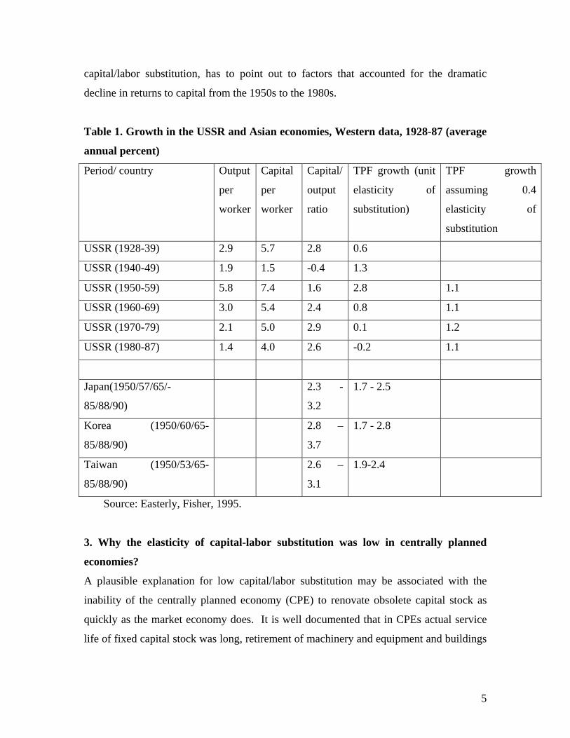
capital/labor substitution, has to point out to factors that accounted for the dramatic

decline in returns to capital from the 1950s to the 1980s.

Table 1. Growth in the USSR and Asian economies, Western data, 1928-87 (average

annual percent)

Period/ country Output

per

worker

Capital

per

worker

Capital/

output

ratio

TPF growth (unit

elasticity of

substitution)

TPF growth

assuming 0.4

elasticity of

substitution

USSR (1928-39) 2.9 5.7 2.8 0.6

USSR (1940-49) 1.9 1.5 -0.4 1.3

USSR (1950-59) 5.8 7.4 1.6 2.8 1.1

USSR (1960-69) 3.0 5.4 2.4 0.8 1.1

USSR (1970-79) 2.1 5.0 2.9 0.1 1.2

USSR (1980-87) 1.4 4.0 2.6 -0.2 1.1

Japan(1950/57/65/-

85/88/90)

2.3 -

3.2

1.7 - 2.5

Korea (1950/60/65-

85/88/90)

2.8 –

3.7

1.7 - 2.8

Taiwan (1950/53/65-

85/88/90)

2.6 –

3.1

1.9-2.4

Source: Easterly, Fisher, 1995.

3. Why the elasticity of capital-labor substitution was low in centrally planned

economies?

A plausible explanation for low capital/labor substitution may be associated with the

inability of the centrally planned economy (CPE) to renovate obsolete capital stock as

quickly as the market economy does. It is well documented that in CPEs actual service

life of fixed capital stock was long, retirement of machinery and equipment and buildings

5

and structures was slow and the average age of equipment was high and growing

(Shmelev and Popov, 1989).

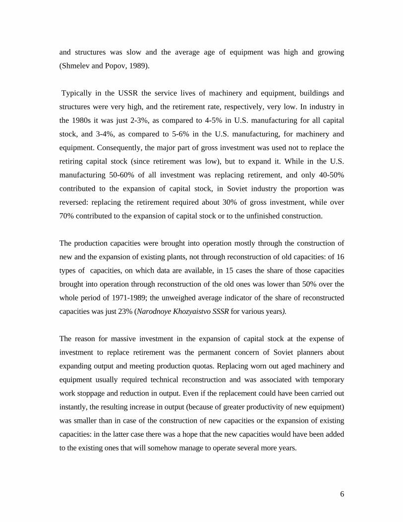
Typically in the USSR the service lives of machinery and equipment, buildings and

structures were very high, and the retirement rate, respectively, very low. In industry in

the 1980s it was just 2-3%, as compared to 4-5% in U.S. manufacturing for all capital

stock, and 3-4%, as compared to 5-6% in the U.S. manufacturing, for machinery and

equipment. Consequently, the major part of gross investment was used not to replace the

retiring capital stock (since retirement was low), but to expand it. While in the U.S.

manufacturing 50-60% of all investment was replacing retirement, and only 40-50%

contributed to the expansion of capital stock, in Soviet industry the proportion was

reversed: replacing the retirement required about 30% of gross investment, while over

70% contributed to the expansion of capital stock or to the unfinished construction.

The production capacities were brought into operation mostly through the construction of

new and the expansion of existing plants, not through reconstruction of old capacities: of 16

types of capacities, on which data are available, in 15 cases the share of those capacities

brought into operation through reconstruction of the old ones was lower than 50% over the

whole period of 1971-1989; the unweighed average indicator of the share of reconstructed

capacities was just 23% (Narodnoye Khozyaistvo SSSR for various years).

The reason for massive investment in the expansion of capital stock at the expense of

investment to replace retirement was the permanent concern of Soviet planners about

expanding output and meeting production quotas. Replacing worn out aged machinery and

equipment usually required technical reconstruction and was associated with temporary

work stoppage and reduction in output. Even if the replacement could have been carried out

instantly, the resulting increase in output (because of greater productivity of new equipment)

was smaller than in case of the construction of new capacities or the expansion of existing

capacities: in the latter case there was a hope that the new capacities would have been added

to the existing ones that will somehow manage to operate several more years.

6

Aged and worn out equipment and structures were thus normally repaired endlessly, until

they were falling apart physically; capital repair expenditure amounted to over 1/3 of annual

investment. The capital stock meanwhile was getting older and was wearing out, the average

age of equipment and structures increased constantly.

The official statistics suggest that the share of investment into the reconstruction of

enterprises (as opposed to the expansion of existing and construction of new enterprises)

increased from 33% in 1980 to 39% in 1985 to 50% in 1989 (Narkhoz, 1989, p.280), but

this is not very consistent with the other official data. For instance, the retirement ratio in

Soviet industry was not only very low (below 2% and about 3% respectively for the

retirement of physically obsolete and retirement of all assets), but mostly falling or stable in

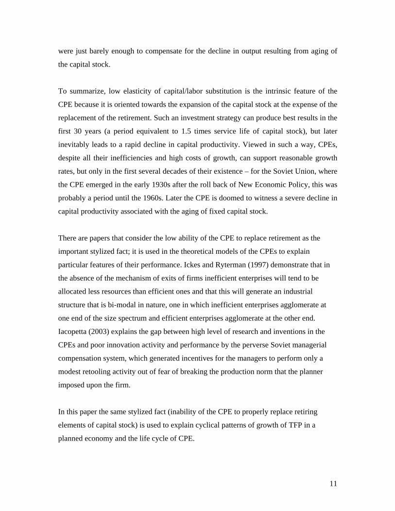
1967-85 (see fig. 1). Only in 1965-67 (right after the economic reform of 1965) and in 1986-

87 (acceleration and restructuring policy) there was a noticeable increase in the retirement

rate.

Fig. 1. Gross investment and retirement in Soviet industry, as a % of fixed capital stock

0

2

4

6

8

10

12

1964

1965

1966

1967

1968

1969

1970

1971

1972

1973

1974

1975

1976

1977

1978

1979

1980

1981

1982

1983

1984

1985

1986

1987

1988

1989

G/KR/K - all R/K - physically obsolete

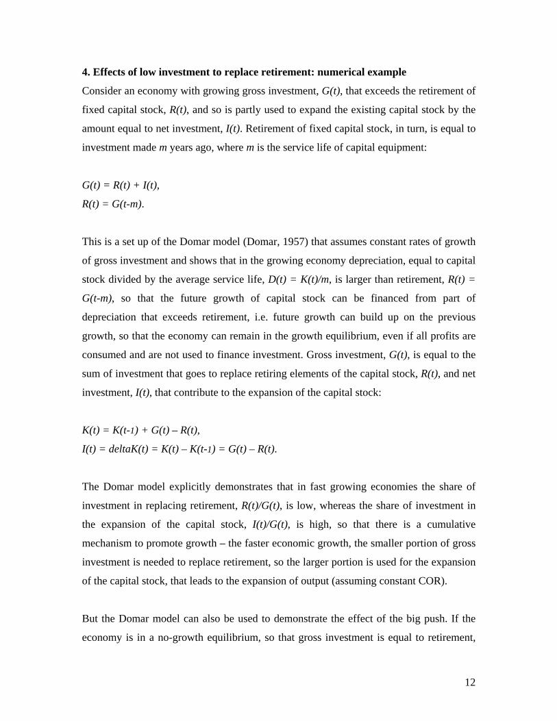
The share of investment to replace retirement in total gross investment also stayed at an

extremely low level of below 20% for the most part of the 1960s-1980s; only in 1965-67

and in 1985-87 there were short-lived increases in this ratio – up to 30% (fig.2).

7

Fig. 2. Share of investment to replace retirement in total gross investment in Soviet industry, %

10

12

14

16

18

20

22

24

26

28

30

1964

1965

1966

1967

1968

1969

1970

1971

1972

1973

1974

1975

1976

1977

1978

1979

1980

1981

1982

1983

1984

1985

1986

1987

1988

1989

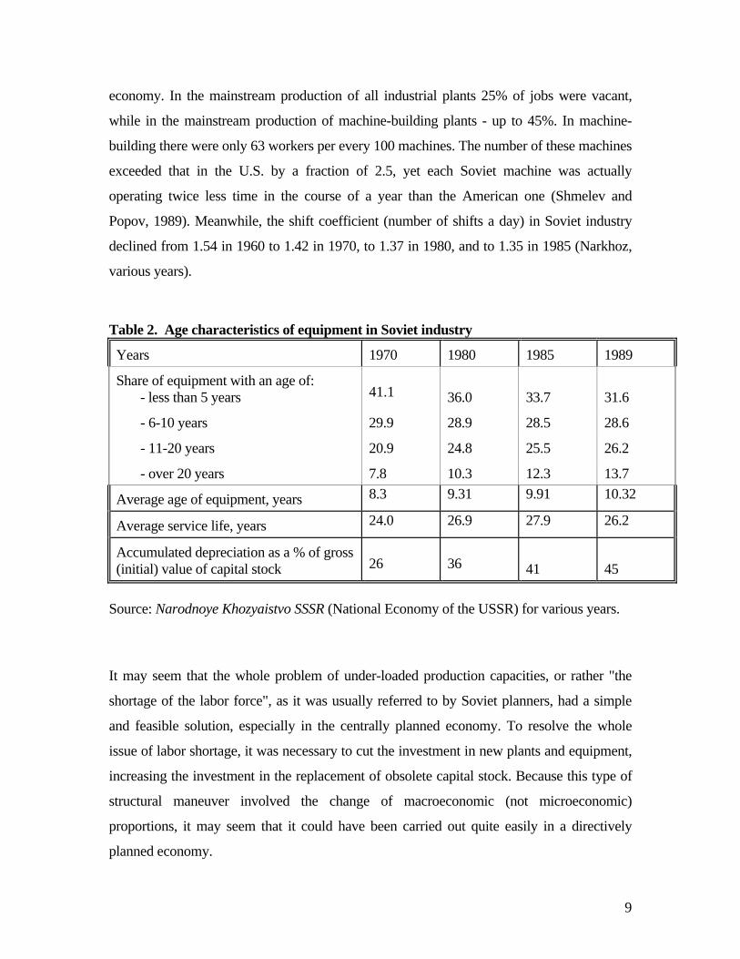
Besides, accumulated depreciation as a percentage of gross value of fixed capital stock

(gross value minus net value, divided by gross value) grew from 26% in 1970 to 45% in

1989, and in some industries, such as steel, chemicals and petrochemicals, exceeded 50% by

the end of 1980s. The average age of industrial equipment increased from 8.3 to 10.3 years

in the 1970s-1980s, and actual average service life was 24-28 years (as compared to a 13

years period, established by norms for depreciation accounting). The share of equipment

over 11 year old increased from 29% in 1970 to 35% in 1980 and to 40% in 1989, while the

share of the equipment used for 20 years and over - from 8 to 14% (table 2).

The planners’ reluctance to modernize existing plants and heavy emphasis on new

construction - a policy that was supposed to increase output as much as possible, in the

long run led to the declining capital productivity. Capacity utilization rate in Soviet

industry was falling rapidly, although official statistics registered only a marginal decrease

(Shmelev and Popov, 1989; Faltsman, 1985; Valtukh, Lavrovsky, 1986). Growing

“shortages” of labor force during the 1970s-1980s may be regarded as a sign of an

increasing share of unloaded production capacities. On the whole, as was estimated by a

Gosplan specialist, the excess capacities, not equipped with labor force, constituted in late

1980s about 1/4 of all capital stock in industry and 1/5 of capital stock in the entire

8

economy. In the mainstream production of all industrial plants 25% of jobs were vacant,

while in the mainstream production of machine-building plants - up to 45%. In machine-

building there were only 63 workers per every 100 machines. The number of these machines

exceeded that in the U.S. by a fraction of 2.5, yet each Soviet machine was actually

operating twice less time in the course of a year than the American one (Shmelev and

Popov, 1989). Meanwhile, the shift coefficient (number of shifts a day) in Soviet industry

declined from 1.54 in 1960 to 1.42 in 1970, to 1.37 in 1980, and to 1.35 in 1985 (Narkhoz,

various years).

Table 2. Age characteristics of equipment in Soviet industry

Years 1970 1980 1985 1989

Share of equipment with an age of: - less than 5 years

41.1

36.0

33.7

31.6

- 6-10 years 29.9 28.9 28.5 28.6

- 11-20 years 20.9 24.8 25.5 26.2

- over 20 years 7.8 10.3 12.3 13.7

Average age of equipment, years 8.3 9.31 9.91 10.32

Average service life, years 24.0 26.9 27.9 26.2

Accumulated depreciation as a % of gross (initial) value of capital stock

26

36

41

45

Source: Narodnoye Khozyaistvo SSSR (National Economy of the USSR) for various years.

It may seem that the whole problem of under-loaded production capacities, or rather "the

shortage of the labor force", as it was usually referred to by Soviet planners, had a simple

and feasible solution, especially in the centrally planned economy. To resolve the whole

issue of labor shortage, it was necessary to cut the investment in new plants and equipment,

increasing the investment in the replacement of obsolete capital stock. Because this type of

structural maneuver involved the change of macroeconomic (not microeconomic)

proportions, it may seem that it could have been carried out quite easily in a directively

planned economy.

9

However, as was already mentioned, excess investment in new construction resulted not

from mismanagement, but from the very idea of directive planning carried out through

setting the production quotas and oriented towards constant increases in output. Shortages

were inevitable in such a system and resulted from disproportions created through central

planning almost by definition, while capital investment were regarded as a major mean of

eliminating the bottlenecks resulting from shortages. So capital investment was diverted to

create new production capacities that would have allowed expanding production of scarce

goods. The whole planning procedure looked like an endless chain of the urgent decisions

forced by emergency shortages of different goods that manifested themselves quicker than

the planners were able to liquidate them.

This was a sort of a vicious circle, a permanent race, in which decisions to make capital

investment were predetermined by existing and newly emerging shortages. It turned out,

therefore, that any attempts to cut the investment in new plant and equipment led to

increased distortions and bottlenecks, resulting, among other things, in the lower capacity

utilization rate, while the increased investment in the construction of new production

facilities contributed to the widening of the gap between job vacancies and the limited

supply of the labor force, also causing the decline in the capacity utilization. Under central

planning, unfortunately, there was no third option.

As a result, the CPE with the inherent and unavoidable low capital/labor elasticity trap

was doomed to survive through a life cycle linked to the service life of fixed capital

stock. Assuming the service life of capital stock is about 20 years, in the first 20 years of

the existence of the CPE the construction of new modern production capacities led to

rapid increases of labor productivity even though the capital/output ratio rose. In the next

10 years production capacities put into operation 20 years earlier started to retire

physically, which contributed to the slow down of the growth rates, but was compensated

by the continuing expansion of fixed capital stock. After 30 years of the existence of the

CPE, it entered the stage of the decline: over half of the capital stock was worn out and

falling apart (but not completely replaced), while the newly created production capacities

10

were just barely enough to compensate for the decline in output resulting from aging of

the capital stock.

To summarize, low elasticity of capital/labor substitution is the intrinsic feature of the

CPE because it is oriented towards the expansion of the capital stock at the expense of the

replacement of the retirement. Such an investment strategy can produce best results in the

first 30 years (a period equivalent to 1.5 times service life of capital stock), but later

inevitably leads to a rapid decline in capital productivity. Viewed in such a way, CPEs,

despite all their inefficiencies and high costs of growth, can support reasonable growth

rates, but only in the first several decades of their existence – for the Soviet Union, where

the CPE emerged in the early 1930s after the roll back of New Economic Policy, this was

probably a period until the 1960s. Later the CPE is doomed to witness a severe decline in

capital productivity associated with the aging of fixed capital stock.

There are papers that consider the low ability of the CPE to replace retirement as the

important stylized fact; it is used in the theoretical models of the CPEs to explain

particular features of their performance. Ickes and Ryterman (1997) demonstrate that in

the absence of the mechanism of exits of firms inefficient enterprises will tend to be

allocated less resources than efficient ones and that this will generate an industrial

structure that is bi-modal in nature, one in which inefficient enterprises agglomerate at

one end of the size spectrum and efficient enterprises agglomerate at the other end.

Iacopetta (2003) explains the gap between high level of research and inventions in the

CPEs and poor innovation activity and performance by the perverse Soviet managerial

compensation system, which generated incentives for the managers to perform only a

modest retooling activity out of fear of breaking the production norm that the planner

imposed upon the firm.

In this paper the same stylized fact (inability of the CPE to properly replace retiring

elements of capital stock) is used to explain cyclical patterns of growth of TFP in a

planned economy and the life cycle of CPE.

11

4. Effects of low investment to replace retirement: numerical example

Consider an economy with growing gross investment, G(t), that exceeds the retirement of

fixed capital stock, R(t), and so is partly used to expand the existing capital stock by the

amount equal to net investment, I(t). Retirement of fixed capital stock, in turn, is equal to

investment made m years ago, where m is the service life of capital equipment:

G(t) = R(t) + I(t),

R(t) = G(t-m).

This is a set up of the Domar model (Domar, 1957) that assumes constant rates of growth

of gross investment and shows that in the growing economy depreciation, equal to capital

stock divided by the average service life, D(t) = K(t)/m, is larger than retirement, R(t) =

G(t-m), so that the future growth of capital stock can be financed from part of

depreciation that exceeds retirement, i.e. future growth can build up on the previous

growth, so that the economy can remain in the growth equilibrium, even if all profits are

consumed and are not used to finance investment. Gross investment, G(t), is equal to the

sum of investment that goes to replace retiring elements of the capital stock, R(t), and net

investment, I(t), that contribute to the expansion of the capital stock:

K(t) = K(t-1) + G(t) – R(t),

I(t) = deltaK(t) = K(t) – K(t-1) = G(t) – R(t).

The Domar model explicitly demonstrates that in fast growing economies the share of

investment in replacing retirement, R(t)/G(t), is low, whereas the share of investment in

the expansion of the capital stock, I(t)/G(t), is high, so that there is a cumulative

mechanism to promote growth – the faster economic growth, the smaller portion of gross

investment is needed to replace retirement, so the larger portion is used for the expansion

of the capital stock, that leads to the expansion of output (assuming constant COR).

But the Domar model can also be used to demonstrate the effect of the big push. If the

economy is in a no-growth equilibrium, so that gross investment is equal to retirement,

12

G(t) = R(t) = G(t-m), but at a certain point experiences a “big push”, so that investment

start exceed annual retirement of fixed capital stock, then growth can be maintained

indefinitely even if all profits are consumed and are not used to finance investment. In

this paper the basic setup of the Domar model is used to demonstrate another effect: the

impact of the “big push” on the growth rates of the economy is not sustainable, if the

ability of the system to invest into the replacement of the retirement of the fixed capital

stock is constrained.

Unlike investment into the expansion of the capital stock (construction of new production

capacities), investment in the replacement of the retirement does not create new jobs. Let

us make a distinction between the actual retirement of capital equipment due to the end of

its service life, G(t-m), and annual investment into the replacement of retirement, R(t).

The reasonable assumption for the market economy would be that investment in the

replacement of retirement (reconstruction of existing production capacities) is higher than

the actual retirement of capital equipment (wear and tear of the capital stock), R(t)>G(t-

m), because machinery and equipment, buildings and structures become not only

physically obsolete, but also technologically obsolete: it may pay off to replace a piece of

machinery before its actual physical retirement by a more technically advanced one.

Suppose, therefore, that investment into the replacement of the retirement is equal to

actual retirement, G(t-m), plus an additional 10% of gross investment, G(t):

R(t) = G(t-m) + 0.1G(t) (1)

Capital stock this year is equal to the capital stock in the previous year, plus net

investment, equal to the difference between gross investment and investment into the

replacement of retirement:

K(t) = K(t-1) + I(t) = K(t-1) + G(t) – R(t) (2)

Gross investment is a constant share of income, Y(t):

13

G(t) = aY(t) (3)

(later it is assumed that a is equal to 5% before the “big push” and 10% afterwards).

Finally, the most important equation is the one that describes the increase in income. The

assumption here is that this increase is proportional to the increase in the fixed capital

stock, deltaK = I(t) = G(t)–R(t), but also depends on the share of investment into the

replacement of retirement in total gross investment, R(t)/G(t):

deltaY = b[G(t) – R(t)]*R(t)/G(t) (4)

The rationale for such a relationship is twofold. First, if the growth of the labor force is

limited, then productivity of the investment into the expansion of capital stock (creation

of new production capacities, i.e. new jobs, requiring new employees) is constrained by

the labor force shortage: the increase in output in newly created production capacities

would be accompanied by the decline in output in the old plants, from where workers will

have to leave in order to take new jobs at the newly created plants. On the contrary, if all

gross investment are used to replace retirement (to reconstruct the existing production

capacities without creating new jobs), so that R(t)=G(t), then R(t)/G(t) is equal to 1

(maximum) and the productivity of new investment is the highest.

Second, if the speed of structural change is high enough as compared to the rate of

retirement of capital stock due to physical wear and tear, so that it requires the re-

allocation of capital and labor from old industries/regions/plants to new ones and this re-

allocation is associated with adjustment costs (re-training of employees, shut down of

physically non-obsolete capacities), the productivity of new investment in the expansion

of production capacities may be lower as compared to investment into the reconstruction

of the old capacities. A certain pace of structural change is necessary in any economy for

the technical progress to proceed. But this pace may be so high that it requires the shut

down of physically non-obsolete enterprises, if the country is catching up rapidly with the

technological leader and/or changes it’s specialization in the international trade. Imagine,

14

for example, that a country switches from export of agricultural output to export of

industrial goods and has to reallocate labor and capital from agriculture to industry. Even

if private returns from investment in industry are greater than from investment into

agriculture, social returns (taking into account adjustment costs) can be lower. Hence, the

productivity of investment into the expansion of fixed capital stock is assumed to be

proportional to the share of investment into the replacement of retirement in total gross

investment, R(t)/G(t).

The last equation is the one that links output in the current year to output in the preceding

year:

Y(t) = Y(t-1) + deltaY(t-1) (5)

Assume now that in the initial year capital stock is equal to 20, output is equal to 20,

gross investment is equal to 1 (the share of gross investment in income is thus 5%),

retirement is also equal to 1, and service life of the capital stock is 20. So the system is

not growing, and maintains stable no-growth equilibrium (growth rates of output are

defined as delta(t)/Y(t) ). After the first 20 years the “big push” occurs – investment in the

year 21 increase to 2, so that the share of investment in income rises to 10%. The

trajectory of the growth rates, assuming b, the productivity of new investment, is equal to

10, is shown at fig. 3 below (the trajectory in the middle) – growth rates increase to 31%

a year right away, then gradually decline in the course of the next 20 years to 13% and

then after some fluctuations stabilize at a level of 16%3.

Growth rates could be better than that, if we change the rule for the investment into the

replacement of retirement, given by equation (1). To get the maximum possible growth

rates, it is necessary to find the optimal investment into the replacement of the retirement

3 For the illustration purposes the year of the “big push” is set as 1930. The assumption that the system was in the no growth equilibrium in 1910-30 is not that far from reality: even though Russian/Soviet output fell from 100% in the 1913 to about 30% in the 1920 and then recovered to about 130% by 1930, fixed capital stock in this period most probably did not change much – investment were generally enough only to replace retirement, not to expand the capital stock.

15

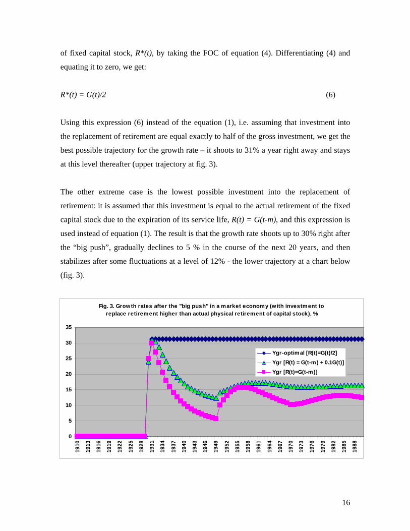
of fixed capital stock, R*(t), by taking the FOC of equation (4). Differentiating (4) and

equating it to zero, we get:

R*(t) = G(t)/2 (6)

Using this expression (6) instead of the equation (1), i.e. assuming that investment into

the replacement of retirement are equal exactly to half of the gross investment, we get the

best possible trajectory for the growth rate – it shoots to 31% a year right away and stays

at this level thereafter (upper trajectory at fig. 3).

The other extreme case is the lowest possible investment into the replacement of

retirement: it is assumed that this investment is equal to the actual retirement of the fixed

capital stock due to the expiration of its service life, R(t) = G(t-m), and this expression is

used instead of equation (1). The result is that the growth rate shoots up to 30% right after

the “big push”, gradually declines to 5 % in the course of the next 20 years, and then

stabilizes after some fluctuations at a level of 12% - the lower trajectory at a chart below

(fig. 3).

Fig. 3. Growth rates after the "big push" in a market economy (w ith investment to replace retirement higher than actual physical retirement of capital stock), %

0

5

10

15

20

25

30

35

1910

1913

1916

1919

1922

1925

1928

1931

1934

1937

1940

1943

1946

1949

1952

1955

1958

1961

1964

1967

1970

1973

1976

1979

1982

1985

1988

Ygr-optimal [R(t)=G(t)/2]Ygr [R(t) = G(t-m) + 0.1G(t)]Ygr [R(t)=G(t-m)]

16

The point of these simulations is to show that in all cases the growth rates after the “big

push” stabilize at a positive level. This is not the case, however, if the assumptions are

slightly modified, so as to allow for the investment into the replacement of retirement of

the fixed capital stock, R(t), to be below the actual physical retirement, G(t-m). Equation

(2) will then have to be modified, so that the increase in the capital stock is equal to gross

investment minus actual retirement, G(t-m), and not the investment into the replacement

of retirement, R(t):

K(t) = K(t-1) + G(t) – G(t-m) (2’)

Equation (4) will have to be modified as well, so that the increase in the fixed capital

stock is defined accordingly:

deltaY = b[G(t) – G(t-m)]*R(t)/G(t) (4’)

Finally, for describing investment into the replacement of retirement, let us use the

simplest rule – a constant fraction of gross investment, c, small enough to make

investment to replace retirement lower than the actual physical retirement of fixed capital

stock:

R(t) = cG(t) (1’)

This equation (1’) replaces the equation (1). As a result, the new trajectories of growth

rates, shown at the chart below (fig. 4), are very different from the ones that were

obtained previously under the assumption that investment into the replacement of the

retirement is higher than actual retirement.

If c is equal to 0.1, i.e. investment into the replacement of the retirement of fixed capital

stock are only 10% of total gross capital investment, then growth rates after the “big

push” increase immediately to 5%, then gradually grow to 9% in the course of next 20

years, but afterwards fall and converge after some fluctuations to a level of 8% (the upper

17

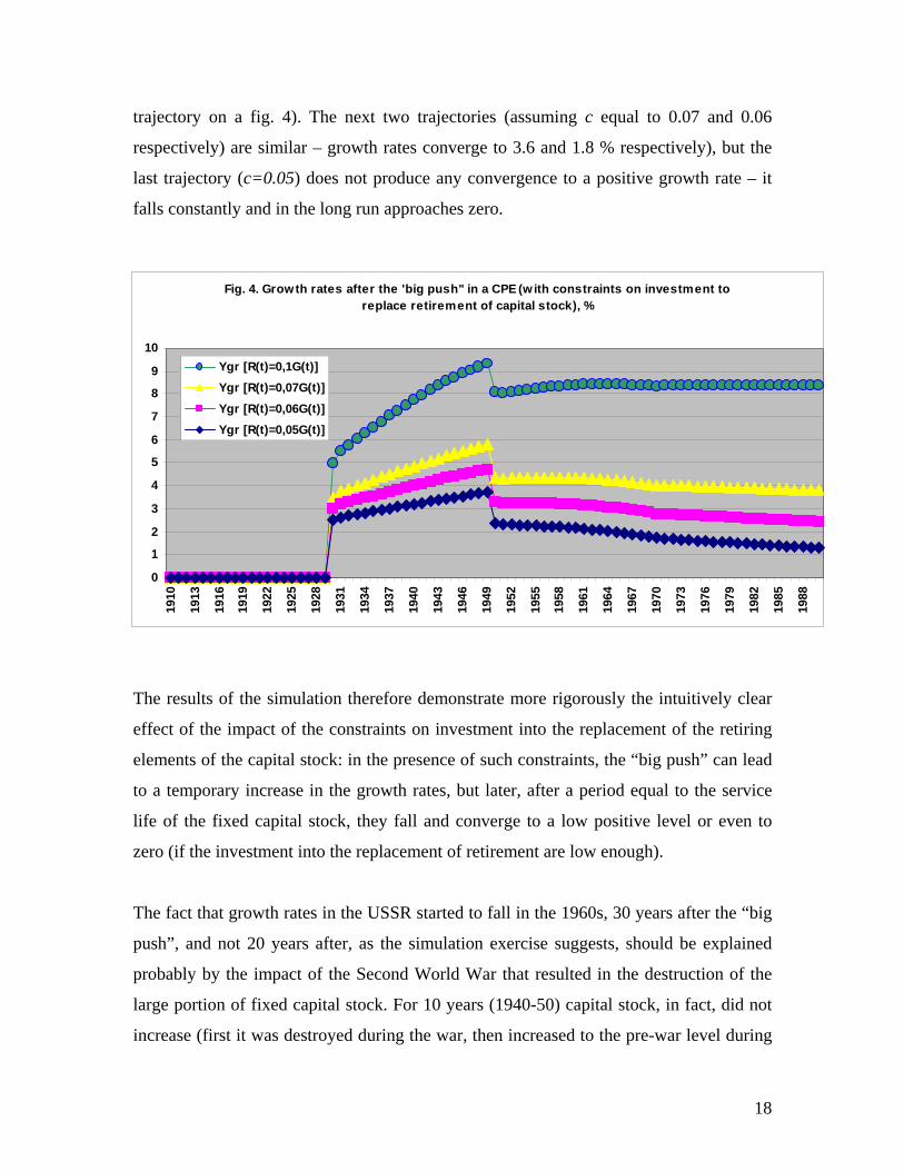
trajectory on a fig. 4). The next two trajectories (assuming c equal to 0.07 and 0.06

respectively) are similar – growth rates converge to 3.6 and 1.8 % respectively), but the

last trajectory (c=0.05) does not produce any convergence to a positive growth rate – it

falls constantly and in the long run approaches zero.

Fig. 4. Growth rates after the 'big push" in a CPE (w ith constraints on investment to replace retirement of capital stock), %

0

1

2

3

4

5

6

7

8

9

10

1910

1913

1916

1919

1922

1925

1928

1931

1934

1937

1940

1943

1946

1949

1952

1955

1958

1961

1964

1967

1970

1973

1976

1979

1982

1985

1988

Ygr [R(t)=0,1G(t)]Ygr [R(t)=0,07G(t)]Ygr [R(t)=0,06G(t)]Ygr [R(t)=0,05G(t)]

The results of the simulation therefore demonstrate more rigorously the intuitively clear

effect of the impact of the constraints on investment into the replacement of the retiring

elements of the capital stock: in the presence of such constraints, the “big push” can lead

to a temporary increase in the growth rates, but later, after a period equal to the service

life of the fixed capital stock, they fall and converge to a low positive level or even to

zero (if the investment into the replacement of retirement are low enough).

The fact that growth rates in the USSR started to fall in the 1960s, 30 years after the “big

push”, and not 20 years after, as the simulation exercise suggests, should be explained

probably by the impact of the Second World War that resulted in the destruction of the

large portion of fixed capital stock. For 10 years (1940-50) capital stock, in fact, did not

increase (first it was destroyed during the war, then increased to the pre-war level during

18

reconstruction), so 10 years should be added to the life cycle of 20 years. Besides, the

average service life of capital stock is a very statistically uncertain indicator. In the 1970s

– 1980s for machinery and equipment the service life was about 25 years (implying a

retirement ratio of 4%) – see table 2, but for the earlier period the statistics is absent. If

the service life in the 1930s-1950s was about 30 years, the peak of the growth rates in the

1950s could be explained even without the impact of the war.

5. Conclusions

The highest rates of growth of labor productivity in the Soviet Union were observed not

in the 1930s (3% annually), but in the 1950s (6%). The TFP growth rates by decades

increased from 0.6% annually in the 1930s to 2.8% in the 1950s and then fell

monotonously becoming negative in the 1980s. The decade of 1950s was thus the

“golden period” of Soviet economic growth. The patterns of Soviet growth of the 1950s

in terms of growth accounting were very similar to the Japanese growth of the 1950s-70s

and Korean and Taiwanese growth in the 1960-80s – fast increases in labor productivity

counterweighted the decline in capital productivity, so that the TFP increased markedly.

However, high Soviet economic growth lasted only for a decade, whereas in East Asia it

continued for three to four decades, propelling Japan, South Korea and Taiwan into the

ranks of developed countries.

This paper offers an explanation for the inverted U-shaped trajectory of labor

productivity and TFP in centrally planned economies (CPEs). It is argued that CPEs

under-invested into the replacement of the retiring elements of the fixed capital stock and

over-invested into the expansion of production capacities. The task of renovating physical

capital contradicted the short-run goal of fulfilling planned targets, and, therefore, Soviet

planners preferred to invest in new capacities instead of upgrading the old ones. Hence,

after the massive investment of the 1930s in the USSR, the highest productivity was

achieved after the period equal to the service life of capital stock (about 20 years) –

before there emerged a need for the massive investment into replacing retirement.

Afterwards, the capital stock started to age rapidly reducing sharply capital productivity

and lowering labor productivity and TFP growth rates.

19

The simulation exercise allows to demonstrate clearly that under very reasonable

assumptions (that the productivity of new investment is proportional to the share of

investment into the reconstruction of existing production capacities in total investment,

and that investment into the reconstruction of these capacities is lower than the actual

retirement due to physical wear and tear) growth rates first increase and than fall to very

low level or even zero after the “big push” – the initial increase in the share of investment

in GDP.

Among many reasons of the decline of the growth rates in the USSR in the 1960s-1980s,

the discussed inability of the centrally planned economy to ensure adequate flow of

investment into the replacement of retirement of fixed capital stock appears to be most

crucial. What is more important, even if these retirement constraints were not the only

reason of the decline in growth rates, they are sufficient to explain the inevitable gradual

decline after 30 years of relatively successful development. To put it differently, the

centrally planned economy is doomed to experience a growth slowdown after three

decades of high growth following the “big push”. In this respect, Chinese relatively short

experience with the CPE (1949-79) looks superior to the Soviet excessively long

experience (1929-91). This is another reason to believe that the transition to the market

economy in the Soviet Union would have been more successful, if it had started in the

1960s.

20

REFERENCES

Bergson, A. 1983. Technological progress. – In: A. Bergson and H. Levine “The Soviet

Economy Towards the Year 2000”, London, UK, George Allen and Unwin, 1983.

Commission of the European Communities. 1990. Stabilization, Liberalization and

Devolution: Assessment of the Economic Situation and Reform Process in the Soviet

Union. December 19, 1990.

Desai, P. 1976. The Production Function and Technical Change in Postwar Soviet

Industry. – American Economic Review, Vol. 60, No. 3, pp. 372-381.

Domar, E. Essays in the Theory of Economic Growth. N.Y., 1957.

Easterly, W., Fisher, S. 1995. The Soviet Economic Decline. – The World Bank

Economic Review, Vol. 9, No.3, pp. 341-71.

Faltsman V. 1985. Proizvodstvenniye Moschnosty. (Production Facilities) – Voprosy

Economiki, 1985, No. 3, p. 47;

Gomulka, S.1977. Slowdown in Soviet Industrial Growth, 1947-1985 Reconsidered. –

European Economic Review, Vol. 10, No.1 (October), pp. 37-49.

Guriev, S., Ickes, B. 2000. Microeconomic Aspects of Economic Growth in Eastern

Europe and the Former Soviet Union, 1950-2000. GDN Growth Project.

Iacopetta, M. (2003). Dissemination of Technology in Market and Planned Economies

School of Economics, Georgia Institute of Technology, Mimeo. June, 2003

Ickes, B. and R. Ryterman (1997). Entry Without Exit: Economic Selection Under

Socialism. Department of Economics. The Pennsylvania State University. Mimeo. 1997.

IMF, WB, OECD, EBRD. 1991. A Study of the Soviet Economy. February 1991. Vol.

1,2,3.

Krugman, P. 1994. The Myth of Asia’s Miracle. – Foreign Affairs, November/December

1994, pp. 62-78.

Narkhoz (Narodnoye Khosyaistvo SSSR), various years, Goskomstat.

Ofer, G. 1987. Soviet economic Growth: 1928-85. – Journal of Economic Literature,

Vol. 25, No. 4 (December), pp. 1767-1833.

Radelet, S., Sachs, J. 1997. Asia’s Reemergence. – Foreign Affairs, November/December

1997, pp. 44-59.

21

Schroeder, G. 1995.Reflections on economic Sovetology. – Post-Soviet Affairs, Vol. 11,

No.3, pp. 197-234.

Shmelev, N., and Popov, V. 1989. The Turning Point: Revitalizing the Soviet Economy.

New York, Doubleday, 1989.

Wang, Yan and Yao Yudong (2001). Sources of China s Economic Growth, 1952-99.

The World Bank, World Bank Institute, Economic Policy and Poverty Reduction

Division July 2001.

Weitzman, M. 1970. Soviet Postwar Economic Growth and Capital-Labor Substitution. –

American Economic Review, Vol. 60, No.5 (December), pp. 676-92.

Young A. 1994. Lessons from the East Asian NICs: A Contrarian View. – European

Economic Review, Vol. 38, No.4, pp. 964-73.

Valtukh, K., Lavrovskyi B. "Proizvodstvennyi Apparat Strany: Ispol'zovaniye i

Rekonstruktsiya" (Production Facilities of a Country: Utilization and Reconstruction). -

EKO, 1986, N2, pp. 17-32.

22

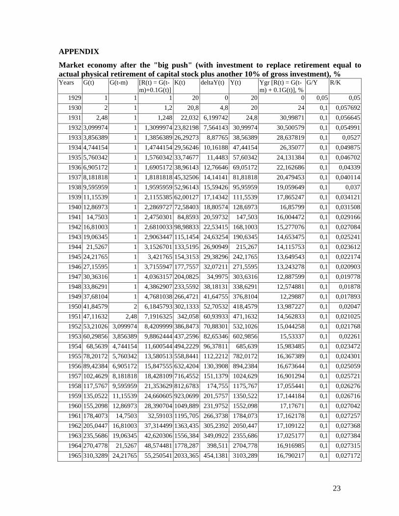
APPENDIX

Market economy after the "big push" (with investment to replace retirement equal to actual physical retirement of capital stock plus another 10% of gross investment), % Years G(t) G(t-m) [R(t) = G(t-

m)+0.1G(t)]K(t) deltaY(t) Y(t) Ygr [R(t) = G(t-

m) + 0.1G(t)], % G/Y R/K

1929 1 1 1 20 0 20 0 0,05 0,051930 2 1 1,2 20,8 4,8 20 24 0,1 0,0576921931 2,48 1 1,248 22,032 6,199742 24,8 30,99871 0,1 0,0566451932 3,099974 1 1,3099974 23,82198 7,564143 30,99974 30,500579 0,1 0,0549911933 3,856389 1 1,3856389 26,29273 8,87765 38,56389 28,637819 0,1 0,05271934 4,744154 1 1,4744154 29,56246 10,16188 47,44154 26,35077 0,1 0,0498751935 5,760342 1 1,5760342 33,74677 11,4483 57,60342 24,131384 0,1 0,0467021936 6,905172 1 1,6905172 38,96143 12,76646 69,05172 22,162686 0,1 0,043391937 8,181818 1 1,8181818 45,32506 14,14141 81,81818 20,479453 0,1 0,0401141938 9,595959 1 1,9595959 52,96143 15,59426 95,95959 19,059649 0,1 0,0371939 11,15539 1 2,1155385 62,00127 17,14342 111,5539 17,865247 0,1 0,0341211940 12,86973 1 2,2869727 72,58403 18,80574 128,6973 16,85799 0,1 0,0315081941 14,7503 1 2,4750301 84,8593 20,59732 147,503 16,004472 0,1 0,0291661942 16,81003 1 2,6810033 98,98833 22,53415 168,1003 15,277076 0,1 0,0270841943 19,06345 1 2,9063447 115,1454 24,63254 190,6345 14,653475 0,1 0,0252411944 21,5267 1 3,1526701 133,5195 26,90949 215,267 14,115753 0,1 0,0236121945 24,21765 1 3,421765 154,3153 29,38296 242,1765 13,649543 0,1 0,0221741946 27,15595 1 3,7155947 177,7557 32,07211 271,5595 13,243278 0,1 0,0209031947 30,36316 1 4,0363157 204,0825 34,9975 303,6316 12,887599 0,1 0,0197781948 33,86291 1 4,3862907 233,5592 38,18131 338,6291 12,574881 0,1 0,018781949 37,68104 1 4,7681038 266,4721 41,64755 376,8104 12,29887 0,1 0,0178931950 41,84579 2 6,1845793 302,1333 52,70532 418,4579 13,987227 0,1 0,020471951 47,11632 2,48 7,1916325 342,058 60,93933 471,1632 14,562833 0,1 0,0210251952 53,21026 3,099974 8,4209999 386,8473 70,88301 532,1026 15,044258 0,1 0,0217681953 60,29856 3,856389 9,8862444 437,2596 82,65346 602,9856 15,53337 0,1 0,022611954 68,5639 4,744154 11,600544 494,2229 96,37811 685,639 15,983485 0,1 0,0234721955 78,20172 5,760342 13,580513 558,8441 112,2212 782,0172 16,367389 0,1 0,0243011956 89,42384 6,905172 15,847555 632,4204 130,3908 894,2384 16,673644 0,1 0,0250591957 102,4629 8,181818 18,428109 716,4552 151,1379 1024,629 16,901294 0,1 0,0257211958 117,5767 9,595959 21,353629 812,6783 174,755 1175,767 17,055441 0,1 0,0262761959 135,0522 11,15539 24,660605 923,0699 201,5757 1350,522 17,144184 0,1 0,0267161960 155,2098 12,86973 28,390704 1049,889 231,9752 1552,098 17,17671 0,1 0,0270421961 178,4073 14,7503 32,59103 1195,705 266,3738 1784,073 17,162178 0,1 0,0272571962 205,0447 16,81003 37,314499 1363,435 305,2392 2050,447 17,109122 0,1 0,0273681963 235,5686 19,06345 42,620306 1556,384 349,0922 2355,686 17,025177 0,1 0,0273841964 270,4778 21,5267 48,574481 1778,287 398,511 2704,778 16,916985 0,1 0,0273151965 310,3289 24,21765 55,250541 2033,365 454,1381 3103,289 16,790217 0,1 0,027172

23

1966 355,7427 27,15595 62,730218 2326,378 516,6863 3557,427 16,649634 0,1 0,0269651967 407,4113 30,36316 71,104292 2662,685 586,9467 4074,113 16,499191 0,1 0,0267041968 466,106 33,86291 80,473508 3048,317 665,797 4661,06 16,342133 0,1 0,0263991969 532,6857 37,68104 90,94961 3490,054 754,2107 5326,857 16,181098 0,1 0,026061970 608,1068 41,84579 102,65647 3995,504 853,267 6081,068 16,018207 0,1 0,0256931971 693,4335 47,11632 116,45967 4572,478 969,0069 6934,335 15,934814 0,1 0,025471972 790,3342 53,21026 132,24368 5230,568 1101,158 7903,342 15,879797 0,1 0,0252831973 900,45 60,29856 150,34356 5980,675 1252,415 9004,5 15,846646 0,1 0,0251381974 1025,691 68,5639 171,13305 6835,233 1425,801 10256,91 15,834316 0,1 0,0250371975 1168,272 78,20172 195,02887 7808,476 1624,712 11682,72 15,840158 0,1 0,0249771976 1330,743 89,42384 222,49811 8916,72 1852,968 13307,43 15,860762 0,1 0,0249531977 1516,039 102,4629 254,06686 10178,69 2114,888 15160,39 15,892541 0,1 0,0249611978 1727,528 117,5767 290,32953 11615,89 2415,366 17275,28 15,932076 0,1 0,0249941979 1969,065 135,0522 331,95869 13253 2759,948 19690,65 15,976281 0,1 0,0250481980 2245,06 155,2098 379,71573 15118,34 3154,929 22450,6 16,022475 0,1 0,0251161981 2560,553 178,4073 434,46255 17244,43 3607,45 25605,53 16,068392 0,1 0,0251941982 2921,298 205,0447 497,17442 19668,56 4125,605 29212,98 16,112167 0,1 0,0252781983 3333,858 235,5686 568,9544 22433,46 4718,57 33338,58 16,152307 0,1 0,0253621984 3805,715 270,4778 651,04931 25588,12 5396,733 38057,15 16,187652 0,1 0,0254431985 4345,388 310,3289 744,86774 29188,65 6171,857 43453,88 16,217339 0,1 0,0255191986 4962,574 355,7427 852,00013 33299,22 7057,244 49625,74 16,240767 0,1 0,0255861987 5668,298 407,4113 974,24119 37993,28 8067,931 56682,98 16,257552 0,1 0,0256421988 6475,092 466,106 1113,6152 43354,75 9220,907 64750,92 16,267504 0,1 0,0256861989 7397,182 532,6857 1272,4039 49479,53 10535,35 73971,82 16,270584 0,1 0,0257161990 8450,717 608,1068 1453,1785 56477,07 12032,91 84507,17 16,266885 0,1 0,02573

24

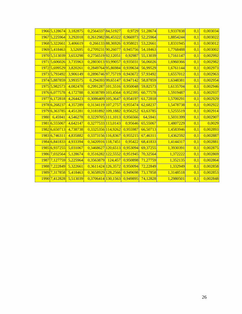
CPE economy after the "big push" (with investment to replace retirement equal to

5% of gross investment), % Years G(t) G(t-m) R(t)=

0.05G(t) K(t) deltaY(t) Y(t) Ygr [R(t)=

0,05G(t)], % G/Y R/K

1929 1 1 1 20 0 20 0 0,05 0,051930 2 1 0,1 21 0,5 20 2,5 0,1 0,0047621931 2,05 1 0,1025 22,05 0,525 20,5 2,625 0,1 0,0046491932 2,1025 1 0,105125 23,1525 0,55125 21,025 2,6890244 0,1 0,0045411933 2,157625 1 0,1078813 24,31013 0,578813 21,57625 2,7529727 0,1 0,0044381934 2,215506 1 0,1107753 25,52563 0,607753 22,15506 2,816769 0,1 0,004341935 2,276282 1 0,1138141 26,80191 0,638141 22,76282 2,8803384 0,1 0,0042461936 2,340096 1 0,1170048 28,14201 0,670048 23,40096 2,9436069 0,1 0,0041581937 2,4071 1 0,120355 29,54911 0,70355 24,071 3,006502 0,1 0,0040731938 2,477455 1 0,1238728 31,02656 0,738728 24,77455 3,0689526 0,1 0,0039921939 2,551328 1 0,1275664 32,57789 0,775664 25,51328 3,1308902 0,1 0,0039161940 2,628895 1 0,1314447 34,20679 0,814447 26,28895 3,1922483 0,1 0,0038431941 2,710339 1 0,135517 35,91713 0,85517 27,10339 3,2529629 0,1 0,0037731942 2,795856 1 0,1397928 37,71298 0,897928 27,95856 3,3129732 0,1 0,0037071943 2,885649 1 0,1442825 39,59863 0,942825 28,85649 3,3722211 0,1 0,0036441944 2,979932 1 0,1489966 41,57856 0,989966 29,79932 3,430652 0,1 0,0035831945 3,078928 1 0,1539464 43,65749 1,039464 30,78928 3,4882146 0,1 0,0035261946 3,182875 1 0,1591437 45,84037 1,091437 31,82875 3,5448612 0,1 0,0034721947 3,292018 1 0,1646009 48,13238 1,146009 32,92018 3,6005476 0,1 0,003421948 3,406619 1 0,170331 50,539 1,20331 34,06619 3,6552337 0,1 0,003371949 3,52695 1 0,1763475 53,06595 1,263475 35,2695 3,7088827 0,1 0,0033231950 3,653298 2 0,1826649 54,71925 0,826649 36,53298 2,3438064 0,1 0,0033381951 3,735963 2,05 0,1867981 56,40521 0,842981 37,35963 2,3074531 0,1 0,0033121952 3,820261 2,1025 0,191013 58,12298 0,85888 38,20261 2,2989533 0,1 0,0032861953 3,906149 2,157625 0,1953074 59,8715 0,874262 39,06149 2,2884875 0,1 0,0032621954 3,993575 2,215506 0,1996787 61,64957 0,889034 39,93575 2,2759869 0,1 0,0032391955 4,082478 2,276282 0,2041239 63,45576 0,903098 40,82478 2,2613784 0,1 0,0032171956 4,172788 2,340096 0,2086394 65,28846 0,916346 41,72788 2,2445833 0,1 0,0031961957 4,264423 2,4071 0,2132211 67,14578 0,928661 42,64423 2,2255172 0,1 0,0031751958 4,357289 2,477455 0,2178644 69,02561 0,939917 43,57289 2,204089 0,1 0,0031561959 4,451281 2,551328 0,222564 70,92557 0,949976 44,51281 2,1802002 0,1 0,0031381960 4,546278 2,628895 0,2273139 72,84295 0,958692 45,46278 2,1537438 0,1 0,0031211961 4,642147 2,710339 0,2321074 74,77476 0,965904 46,42147 2,1246039 0,1 0,0031041962 4,738738 2,795856 0,2369369 76,71764 0,971441 47,38738 2,0926538 0,1 0,0030881963 4,835882 2,885649 0,2417941 78,66787 0,975116 48,35882 2,0577555 0,1 0,0030741964 4,933394 2,979932 0,2466697 80,62133 0,976731 49,33394 2,0197577 0,1 0,003061965 5,031067 3,078928 0,2515533 82,57347 0,976069 50,31067 1,9784946 0,1 0,003046

25

1966 5,128674 3,182875 0,2564337 84,51927 0,9729 51,28674 1,9337838 0,1 0,0030341967 5,225964 3,292018 0,2612982 86,45322 0,966973 52,25964 1,8854244 0,1 0,0030221968 5,322661 3,406619 0,266133 88,36926 0,958021 53,22661 1,8331945 0,1 0,0030121969 5,418463 3,52695 0,2709231 90,26077 0,945756 54,18463 1,7768488 0,1 0,0030021970 5,513039 3,653298 0,2756519 92,12051 0,92987 55,13039 1,7161147 0,1 0,0029921971 5,606026 3,735963 0,2803013 93,99057 0,935031 56,06026 1,6960366 0,1 0,0029821972 5,699529 3,820261 0,2849764 95,86984 0,939634 56,99529 1,6761144 0,1 0,0029731973 5,793492 3,906149 0,2896746 97,75719 0,943672 57,93492 1,6557012 0,1 0,0029631974 5,887859 3,993575 0,294393 99,65147 0,947142 58,87859 1,6348381 0,1 0,0029541975 5,982573 4,082478 0,2991287 101,5516 0,950048 59,82573 1,6135704 0,1 0,0029461976 6,077578 4,172788 0,3038789 103,4564 0,952395 60,77578 1,5919487 0,1 0,0029371977 6,172818 4,264423 0,3086409 105,3647 0,954197 61,72818 1,5700291 0,1 0,0029291978 6,268237 4,357289 0,3134119 107,2757 0,955474 62,68237 1,5478738 0,1 0,0029221979 6,363785 4,451281 0,3181892 109,1882 0,956252 63,63785 1,5255519 0,1 0,0029141980 6,45941 4,546278 0,3229705 111,1013 0,956566 64,5941 1,5031399 0,1 0,0029071981 6,555067 4,642147 0,3277533 113,0143 0,95646 65,55067 1,4807229 0,1 0,00291982 6,650713 4,738738 0,3325356 114,9262 0,955987 66,50713 1,4583946 0,1 0,0028931983 6,746311 4,835882 0,3373156 116,8367 0,955215 67,46311 1,4362592 0,1 0,0028871984 6,841833 4,933394 0,3420916 118,7451 0,95422 68,41833 1,4144317 0,1 0,0028811985 6,937255 5,031067 0,3468627 120,6513 0,953094 69,37255 1,3930391 0,1 0,0028751986 7,032564 5,128674 0,3516282 122,5552 0,951945 70,32564 1,372222 0,1 0,0028691987 7,127759 5,225964 0,3563879 124,457 0,950898 71,27759 1,352135 0,1 0,0028641988 7,222849 5,322661 0,3611424 126,3572 0,950094 72,22849 1,332949 0,1 0,0028581989 7,317858 5,418463 0,3658929 128,2566 0,949698 73,17858 1,3148518 0,1 0,0028531990 7,412828 5,513039 0,3706414 130,1563 0,949895 74,12828 1,2980501 0,1 0,002848

26