causal inference without balance checking: coarsened exact ...causal inference without balance...

doi:10.1093/pan/mpr013

Causal Inference without Balance Checking:Coarsened Exact Matching

Stefano M. Iacus

Department of Economics, Business and Statistics, University of Milan, Via Conservatorio 7,

I-20124 Milan, Italy

e-mail: [email protected]

Gary King

Institute for Quantitative Social Science, Harvard University, 1737 Cambridge Street, Cambridge,

MA 02138

e-mail: [email protected] (corresponding author)

Giuseppe Porro

Department of Economics and Statistics, University of Trieste, P.le Europa 1, I-34127 Trieste, Italy

e-mail: [email protected].

We discuss a method for improving causal inferences called ‘‘Coarsened Exact Matching’’ (CEM), and the new

‘‘Monotonic Imbalance Bounding’’ (MIB) class of matching methods from which CEM is derived. We summarize

what is known about CEM and MIB, derive and illustrate several new desirable statistical properties of CEM, and

then propose a variety of useful extensions. We show that CEM possesses a wide range of statistical properties

not available in most other matching methods but is at the same time exceptionally easy to comprehend and

use. We focus on the connection between theoretical properties and practical applications. We also make

available easy-to-use open source software for R, Stata, and SPSS that implement all our suggestions.

1 Introduction

Observational data are often inexpensive to collect, at least compared to randomized experiments, and soare typically in plentiful supply. However, key aspects of the data generation process—especially thetreatment assignment mechanism—are unknown or ambiguous and in any event are not controlled bythe investigator. This generates the central dilemma of the field, which we might summarize as follows:information, information everywhere, nor a datum to trust (with apologies to Samuel Taylor Coleridge).

Matching is a nonparametric method of controlling for the confounding influence of pretreatment con-trol variables in observational data. The key goal of matching is to prune observations from the data so thatthe remaining data have better balance between the treated and control groups, meaning that the empiricaldistributions of the covariates (X) in the groups are more similar. Exactly balanced data mean that con-trolling further for X is unnecessary (since it is unrelated to the treatment variable), and so a simple dif-ference in means on the matched data can estimate the causal effect; approximately balanced data requirecontrolling for X with a model (such as the same model that would have been used without matching), butthe only inferences necessary are those relatively close to the data, leading to less model dependence andreduced statistical bias than without matching (Ho et al. 2007).

Authors’ note: Open source R, Stata, and SPSS software to implement the methods described herein (called CEM) is available athttp://gking.harvard.edu/cem; the CEM algorithm is also available via a standard interface offered in the R package MatchIt. Thanksto Erich Battistin, Nathaniel Beck, Matt Blackwell, Andy Eggers, Adam Glynn, Justin Grimmer, Jens Hainmueller, Ben Hansen,Kosuke Imai, Guido Imbens, Fabrizia Mealli, Walter Mebane, Clayton Nall, Enrico Rettore, Jamie Robins, Don Rubin, Jas Sekhon,Jeff Smith, Kevin Quinn, and Chris Winship for helpful comments. All information necessary to replicate the results in this paperappear in Iacus, King, and Porro (2011b).

� The Author 2011. Published by Oxford University Press on behalf of the Society for Political Methodology.All rights reserved. For Permissions, please email: [email protected]

Political Analysis Advance Access published August 23, 2011 by guest on A

ugust 24, 2011pan.oxfordjournals.org

Dow

nloaded from

http://pan.oxfordjournals.org/

The central dilemma means that model dependence and statistical bias are usually much bigger problemsthan large variances.1 Unfortunately, most matching methods seem designed for the opposite problem.They guarantee the matched sample size ex ante (thus fixing most aspects of the variance) and producesome level of reduction in imbalance between the treated and control groups (hence reducing bias andmodel dependence) only as a consequence and only sometimes. That is, the less important criterion isguaranteed by the procedure, and any success at achieving the most important criterion is uncertain andmust be checked ex post. Because the methods are not designed to achieve the goal set out for them,numerous applications of matching methods fail the check and so need to be repeatedly tweaked and rerun.

This disconnect gives rise to the most difficult problem in real empirical applications of matching: inmany observational data sets, finding a matching solution that improves balance between the treated andcontrol groups is easy for most covariates, but the result often leaves balance worse for some other var-iables at the same time. Thus, analysts are left with the nagging worry that all their ‘‘improvements’’ inapplying matching may actually have increased bias and model dependence.

Continually checking balance, rematching, and checking again until balance is improved on all var-iables is the best current practice with most existing matching algorithms. The process needs to be repeatedmultiple times because any change in the matching algorithm may alter balance in unpredictable ways onany or all variables. Perhaps the difficulty in following best practices in this field explains why manyapplied articles do not measure or report levels of imbalance at all and appear to run some chosen matchingalgorithm only once. Moreover, even when balance is checked and reported, at best a table comparingmeans in the treatment and control groups is included. Imbalance due to differences in variances, ranges,covariances, and higher order interactions are typically ignored. This of course is a real mistake since anyone application of most existing matching algorithms is not guaranteed (without balance checking) to doany good at all. Of course, it is hard to blame applied researchers who might reasonably expect thata method touted for its ability to reduce imbalance might actually do so when used once.

The problem stems from the fact that widely used current methods, such as propensity score and Maha-lanobis matching, are members of the class of matching methods known as ‘‘equal percent bias reducing’’(EPBR), which does not guarantee any level of imbalance reduction in any given data set; its propertiesonly hold on average across samples and even then only by assuming a set of normally unverifiable as-sumptions about the data generation process. In any application, a single use of these techniques canincrease imbalance and model dependence by any amount.

To avoid these and other problems with EPBR methods, Iacus, King, and Porro (2011) introduce a newgeneralized class of matching methods known as ‘‘Monotonic Imbalance Bounding’’ (MIB). We discussa particular member of the MIB class of matching methods that Iacus, King, and Porro (2011) call ‘‘Coars-ened Exact Matching’’ (CEM). CEM works in sample and requires no assumptions about the data gen-eration process (beyond the usual ignorability assumptions). More importantly, CEM and other MIBmethods invert the process and thus guarantee that the imbalance between the matched treated and controlgroups will not be larger than the ex ante user choice. This level is chosen by the user on the basis ofspecific, intuitive substantive information, which they demonstrably have. (If you understand the trade-offs in drawing a histogram, you will understand how to use this method.) With MIB methods, improve-ments in the bound on balance for one covariate can be studied and improved in isolation as it will have noeffect on the maximum imbalance of each of the other covariates.

CEM-based causal estimates possess a large variety of other powerful statistical properties as well.Some of these are proven in Iacus, King, and Porro (2011) and others are demonstrated here for the firsttime. In a large variety of real and simulated data sets, including data that meet the assumptions made byEPBR methods, Iacus, King, and Porro (2009, 2011) and King et al. (2011) show that CEM dominatescommonly used existing (EPBR and other) matching methods in its ability to reduce imbalance, modeldependence, estimation error, bias, variance, mean square error, and other criteria. We summarize theproperties of CEM here and then introduce a variety of extensions that make the method more widelyapplicable in practice.

1As Rubin (2006) writes, ‘‘First, since it is generally not wise to obtain a very precise estimate of a drastically wrong quantity, theinvestigator should be more concerned about having an estimate with small bias than one with small variance. Second, since in manyobservational studies the sample sizes are sufficiently large that sampling variances of estimators will be small, the sensitivity ofestimators to biases is the dominant source of uncertainty.’’

2 Stefano M. Iacus et al.

by guest on August 24, 2011

pan.oxfordjournals.orgD

ownloaded from


CEM can thus be thought of as an easy first line of defense in protecting users from the threats to validity inmaking causal inferences. The method can also used with other existing methods so that the combined methodinherits the properties shown here apply to CEM. In what follows, we introduce our notation and setup (Sec-tion 2), describe CEM (Section 3), discuss the properties of CEM (Section 4), and extend CEM in varioususeful ways (Section 5). We then offer an empirical illustration to show how it works in practice (Section 6)and conclude with a discussion of what can go wrong when using this approach (Section 7). All data and codenecessary to replicate the results in this paper appear in Iacus, King, and Porro (2011b).

2 Preliminaries

This section describes our setup. It includes our notation, definitions of our target quantities of interest,some simplifying assumptions, a brief summary of existing matching methods and postestimation match-ing, what to do when some treated units cannot be matched, a general characterization of error in esti-mating the target quantities, and how to measure imbalance.

2.1 Notation

Consider a sample of n < N units drawn from a population of size N. Let Ti denote an indicator variable forunit i that takes on value 1 if unit i is a member of the ‘‘treated’’ group and 0 if i is a member of the‘‘control’’ group. The observed outcome variable is Yi 5 TiYi(1) 1 (12 Ti)Yi(0), where Yi(0) is the potentialoutcome for observation i if the unit does not receive treatment and Yi(1) is the potential outcome if the(same) unit receives treatment. For each observed unit, Yi(0) is unobserved if i receives treatment and Yi(1)is unobserved if i does not receive treatment.

To compensate for the observational data problem where the treated and control groups are not nec-essarily identical before treatment (and, lacking random assignment, not the same on average), matchingestimators attempt to control for pretreatment covariates. For this purpose, we denote X5 (X1, X2, . . . Xk)as a k-dimensional data set, where each Xj is a column vector of observed values of pretreatment variablej for the n sample observations (possibly drawn from a population, of size N). That is, X5 [Xij, i5 1, . . ., n,j 5 1, . . ., k]. Let T 5 {i: Ti 5 1} be the set of indexes for the treated units and nT 5 #T be a count of theelements of this set; similarly C 5 {i: Ti 5 0}, nC 5 #C for the control units, with nT 1 nC 5 n. Let Xi 5

(Xi1, . . ., Xik) be the vector of covariates for observation i. We denote by mT and mC the number of treatedand control units matched by some method. Let MT 4 T and MC4 C be the sets of indexes of the matchedunits in the two groups.

2.2 Quantities of Interest

As usual, the treatment effect for unit i, TEi 5 Yi(1) 2 Yi(0), is unobserved. Many relevant causal quantitiesof interest are averages of TEi over different subsets of units and so must be estimated. The most commoninclude the sample (SATT) and population (PATT) average treatment effect on the treated:

SATT51

nT

Xi2T

TEi; PATT51

NT

Xi2T �

TEi;

where T * is the set of indexes of treated units in the whole population and NT 5 #T * (see Imbens 2004;Morgan and Winship 2007).

Although SATT is a quantity of interest in and of itself, without regard to a population beyond thesample data, if the sample is randomly drawn from the relevant population, E(SATT) 5 PATT (wherethe expected value operator averages over repeated samples).

2.3 Simplifying Assumptions

First, similar to the ‘‘no omitted variable bias’’ assumption in the social sciences, we make the standardignorability assumption: conditional onX, the treatment variable is independent of the potential outcomes:Tiv{Yi(0), Yi(1)}jX.

Second, matching-based estimators tend to focus on SATT (or PATT) so that if they choose to retain alltreated units, and prune only control units, the target quantity of interest remains the same. Thus, for each

3Causal Inference without Balance Checking



ownloaded from


observation, Yi(1) is always observed, whereas Yi(0) is always estimated (by choosing values from thecontrol units via some matching algorithm or applying some model). Section 2.6 discusses what todo when the analyst chooses to prune treated units when no reasonable match exists among the poolof available controls.

2.4 Existing Matching Methods

This section outlines the most commonly used matching methods. To begin, one-to-one exact matchingestimates the unobserved Yi(0), corresponding to each observed treated unit i (with outcome value Yi andcovariate values Xi), with the outcome value of a control unit (denoted Y‘ with covariate values X‘),chosen such that X‘ 5Xi. We denote the resulting estimate of Yi(0) as Yið0Þ. To increase efficiency,the alternative exact matching algorithm uses all control units that match each treated unit (i.e., all Xi

such that X‘ 5Xi).Unfortunately, inmost real applications withcovariates sufficiently rich tomake ignorabilityassumptions

plausible, insufficient units can be exactly matched. Thus, analysts must choose one of the existing approx-imate matching methods, the best practice for which involves two separate steps. The first step drops treatedand control units outside the common empirical support of both groups since including them would requireunreasonable extrapolation far from the data. The second step then matches the treated unit to some controlobservation X that, if not exactly X, is close by some metric. The second step of most existing approximatematching procedures can be distinguished by the choice of metric. For example, nearest neighbor Mahala-nobis matching chooses the closest control unit to each treated unit (among those within the common em-pirical support) using the Mahalanobis distance metric. For another example, nearest neighbor propensityscore matching first summarizes the vector of covariate values for an observation by the scalar propensityscore,which is theprobabilityof treatmentgiventhevectorofcovariates, estimated insomeway, typicallyviaa simple logit model.Then, the closest control toeach treated unit isusedasa match, with the distancedefinedby the absolute difference between the two scalar propensity score values. Other options include optimal,subclassification,geneticalgorithm,andotherprocedures.Since thesecondstep inexistingalgorithmsdonotguarantee an improvement in balance except under specialized conditions, the degree of imbalance must bemeasured, the matching algorithm must be respecified, and imbalance must be checked again, etc., untila satisfactory solution is reached. (For example, the correct specification of the propensity score is not in-dicated by measures of fit, only by whether matching on it achieved balance.)

An additional problem for existing approximate matching methods is that most of the technologies usedfor matching in the second step are unhelpful for completing the first step. For example, the propensityscore can be used to find the area of extrapolation only after we know that the correct propensity scoremodel has been used. However, the only way to verify that the correct propensity score model has beenspecified is to check whether matching on it produces balance between the treated and control groups onthe relevant covariates. But balance cannot be reliably checked until the region of extrapolation has beenremoved. To avoid this type of infinite regress, researchers could use entirely different technologies for thefirst step, such as kernel density estimation (Heckman, Ichimura, and Todd 1997) or dropping control unitsoutside the hyperrectangle (Iacus and Porro 2009) or convex hull (King and Zeng 2006) of the treatedunits. In practice, most published applications skip the first step entirely and instead match all treated units,which is not advisable. The method we introduce below avoids these problems by satisfying both stepssimultaneously in the same algorithm.

2.5 Postmatching Estimation

Matching methods are data preprocessing algorithms, not statistical estimators. Thus, after preprocessing,some type of estimator must be applied to the data to make causal inferences. For example, if one-to-oneexact matching is used, then a simple difference in means between Y in the treated and control groupsprovides a fully nonparametric estimator of the causal effect. When the treated and control groups do notmatch exactly, the estimator will necessarily incorporate some modeling assumptions designed to span theremaining differences, and so results will be model dependent to some degree (King and Zeng 2007).Preprocessing via matching can greatly reduce the degree of modeling necessary and thus also the degreeof model dependence (Ho et al. 2007).




ownloaded from


Under a matching method that produces a one-to-one match (or, in general, any match that has a fixedpositive number of treated and control units across strata), any analysis method that might have beenappropriate without matching (such as some type of regression model or specially designed nonparametricmethods; Abadie and Imbens 2007) can alternatively be used on the matched data set with the benefit ofhaving a lower risk of model dependence (Ho et al. 2007).

When different numbers of control units are matched to each treated unit—or, in general, if differentnumbers of treated and control units appear in different strata, as in exact matching—the analysis modelmust weight or adjust for the different stratum sizes. In this situation, the simplest SATT estimator isa weighted difference in means between the treated and control groups or equivalently a weighted linearregression of Yon T. We can go further by trying to span the remaining imbalance via a weighted regressionof Y on T and X. In either regression, the coefficient on T is our SATT estimate. Alternatively, to avoid theimplicit constant treatment effect assumption of the regression approach, we can apply a statistical modelwithin each stratum without weights and average the results across stratum with appropriate weights; whenfew observations exist within each stratum, a Bayesian, empirical Bayes, or random effects model can beapplied in the same way. Finally, nonlinear (or linear) models may also be fit to all the data and used topredict, for each treated unit, the unobserved potential outcome under control Yi(0) given its observedcovariate values Xi, with the treated unit-level estimated causal effects averaged over all treated units.For an example of an implementation of these approaches, see Iacus, King, and Porro (2009).

2.6 When Matches for All Treated Units Do Not Exist

When one or more treated units have no reasonable matches among the set of available controls, standardapproaches will lead to unacceptably high levels of model dependence. In this situation, three options areavailable with any matching method. First, we can decide that the data include insufficient information toestimate the target causal effect and give up, producing no inference at all. Second, we can create controlsby extrapolating from some given model, although leaving us with high levels of model dependence. Orfinally, we can change the estimand to the local SATT, that is the treatment effect averaged over only thesubset of treated units for which good matches exist among available controls. This third approach is oftenused in applications, such as when applying propensity score or Mahalanobis matching with calipers.

The recognized best practice in the literature currently is to eliminate the extrapolation region as a sep-arate prior step and then to match. This procedure deletes treated units without good matches and so isa version of the third option of changing the estimand. This choice is reasonable so long as one is trans-parent about the choice and the consequences in terms of the new set of treated units over which the causaleffect is defined (as, e.g., Crump et al. 2009). The same change in the quantity of interest is common inother methods for observational data, such as local average treatment effects and regression discontinuitydesigns (Imbens and Angrist 1994). The practice is even similar to most randomized experiments, whichdo not select subjects randomly, and so have an estimand that is also defined over a somewhat arbitrary setof units (such as patients who happen to show up at a hospital and agree to be enrolled in a study or thosewho fit conditions researchers believe will demonstrate larger causal effects).

However, most published applications of standard matching methods do not eliminate the extrapolationregion and instead match at all costs regardless of whether reasonable matches exist among the controlunits. In these studies, analysts are effectively taking the second option and producing highly model de-pendent inferences, but without necessarily even knowing it.

We also offer here a more general way to think about this problem, following Iacus, King, and Porro(2011). Thus, we first partition the nT treated units into the mT < nT units, which can be matched well fromthe set of controls, and the nT 2 mT units, which involve extreme counterfactuals (i.e., extrapolations) farfrom the treated units. (Unlike the matching method we introduce below, most standard methods requirea separate prior step to accomplish this, such as the convex hull or hyperrectangle; see Section 2.4.) Then,we match the data in the first subset with acceptable controls to produce a ‘‘local SATT,’’ say smT

. Then, forthe rest of the treated units, we extrapolate via some model estimated on the matched units to obtain virtualcontrol units for the unmatched treated units and produce an (necessarily model dependent) estimatesnT2mT

. Finally, we calculate the overall SATT estimate snT as the weighted mean of the two estimates:




ownloaded from


snT 5smT

� mT1snT2mT� ðnT2mTÞ

nT: ð1Þ

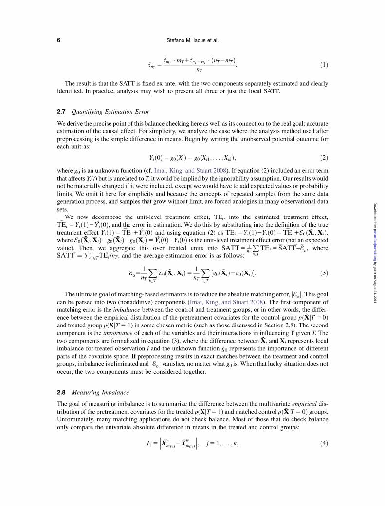
The result is that the SATT is fixed ex ante, with the two components separately estimated and clearlyidentified. In practice, analysts may wish to present all three or just the local SATT.

2.7 Quantifying Estimation Error

We derive the precise point of this balance checking here as well as its connection to the real goal: accurateestimation of the causal effect. For simplicity, we analyze the case where the analysis method used afterpreprocessing is the simple difference in means. Begin by writing the unobserved potential outcome foreach unit as:

Yið0Þ5 g0ðXiÞ5 g0ðXi1; . . . ;XikÞ; ð2Þ

where g0 is an unknown function (cf. Imai, King, and Stuart 2008). If equation (2) included an error termthat affects Yi(t) but is unrelated to T, it would be implied by the ignorability assumption. Our results wouldnot be materially changed if it were included, except we would have to add expected values or probabilitylimits. We omit it here for simplicity and because the concepts of repeated samples from the same datageneration process, and samples that grow without limit, are forced analogies in many observational datasets.

We now decompose the unit-level treatment effect, TEi, into the estimated treatment effect,TEi^

5 Yið1Þ2Yið0Þ, and the error in estimation. We do this by substituting into the definition of the truetreatment effect Yið1Þ5TE^i1Yið0Þ and using equation (2) as TEi 5 Yið1Þ2Yið0Þ5TEi

^1E0ðXi;XiÞ,

where E0ðXi;XiÞ[g0ðXiÞ2g0ðXiÞ5 Yið0Þ2Yið0Þ is the unit-level treatment effect error (not an expectedvalue). Then, we aggregate this over treated units into SATT5 1

nT

Pi2T

TEi 5 SATT^+e�o, whereSATT^¼

P12TTEi^/nT , and the average estimation error is as follows:

e�o[1

nT

Xi2T

E0ðXi;XiÞ51

nT

Xi2T

½g0ðXiÞ2g0ðXiÞ�: ð3Þ

The ultimate goal of matching-based estimators is to reduce the absolute matching error, je�oj. This goalcan be parsed into two (nonadditive) components (Imai, King, and Stuart 2008). The first component ofmatching error is the imbalance between the control and treatment groups, or in other words, the differ-ence between the empirical distribution of the pretreatment covariates for the control group pðXjT5 0Þand treated group p(XjT 5 1) in some chosen metric (such as those discussed in Section 2.8). The secondcomponent is the importance of each of the variables and their interactions in influencing Y given T. Thetwo components are formalized in equation (3), where the difference between Xi and Xi represents localimbalance for treated observation i and the unknown function g0 represents the importance of differentparts of the covariate space. If preprocessing results in exact matches between the treatment and controlgroups, imbalance is eliminated and

��e�o�� vanishes, no matter what g0 is. When that lucky situation does notoccur, the two components must be considered together.

2.8 Measuring Imbalance

The goal of measuring imbalance is to summarize the difference between the multivariate empirical dis-tribution of the pretreatment covariates for the treated p(XjT 5 1) and matched control pðXjT5 0Þ groups.Unfortunately, many matching applications do not check balance. Most of those that do check balanceonly compare the univariate absolute difference in means in the treated and control groups:

I1 5�� Xw

mT ; j2 �X

wmC; j

��; j5 1; . . . ; k; ð4Þ




ownloaded from


where �XwmT ; j

and �XwmC; j

denote weighted means of variable Xj for the groups of mT treated units and mC

control units matched, with weights appropriate to each matching method.Sometimes researchers argue that only matching the mean is necessary because most analysis models

used after or in place of matching (such as regression) only adjust for the mean. However, the purpose ofmatching is to reduce model dependence, and so it does not make sense to assume that the analysis modelis correct, as implied by this argument; for model independent inferences, matching as much of the entireempirical distribution as possible is the goal.

A few have measured imbalance in univariate moments, univariate density plots, propensity score sum-mary statistics, or the average of the univariate differences between the empirical quantile distributions(Rubin 2001; Austin and Mamdani 2006; Imai, King, and Stuart 2008). Except for the occasional dis-cussion about using the differences in covariances, most researchers ignore all aspects of multivariatebalance not represented in these simple variable-by-variable summaries. Unfortunately, improving oncurrent practice by applying existing methods of comparing multivariate histograms—such as Pearson’sv2, Fisher’s G2, or models for contingency tables—would typically work poorly because of the numerouszero cell values.

An alternative approach introduced in Iacus, King, and Porro (2011) is to measure the multivariatedifferences between p(XjT 5 1) and pðXjT5 0Þ via an L1 distance, fixing the bin size to that for themedian L1 for all possible binnings on the raw data. (If prior information indicates that some variablesare more important than others in predicting the outcome, one might choose to use more bins for thatvariable. Either way, the bin sizes must be defined ex ante and not necessarily related to any matchingmethod, including our proposal.2)

Let H(X1) be the set of distinct values generated by binning on variable X1—the set of intervals intowhich the support of variable X1 has been cut. Then, the multidimensional histogram is constructed fromthe set of cells generated by the Cartesian product H(X1)�. . .�H(Xk) 5 H(X). Let f and g be the relativeempirical frequency distributions for the treated and control groups. Let f‘1...‘k be the relative frequency forobservations belonging to the cell with coordinates ‘1; . . . ; ‘k of the multivariate cross-tabulation of thetreated units and g‘1...‘k for the control units.

Definition 1 (Iacus, King, and Porro 2011).

The multivariate imbalance measure is

L1ðf ; gÞ51

2

X‘1...‘k2HðXÞ

��f‘1...‘k2g‘1...‘k��: ð5Þ

Thus, the typically huge number of empty cells do not affect L1(f, g), and the summation in equation (5)never has more than n nonzero terms. The relative frequencies also control for potentially different samplesizes between the groups. Denote by f m and gm the empirical frequencies for matched treated and controlgroups corresponding to the unmatched f and g frequencies and use the same discretization for both thetreated and the control units. Then, a good matching method will have L1(f m, gm) <L1( f, g). The values ofL1 are easily interpetable: if the two distributions of data are completely separated (up to the fine coars-ening of the histogram), then L1 5 1; if the two distributions overlap exactly, then L1 5 0. In all othercases, L1 2 (0, 1). The values of L1 provide useful relative information; if, for example, L1 5 0.6, thenonly 40% of the density of the two histograms overlap. This measure is relative because its meaning isconditional on the data set and chosen covariates.

2Although this initial choice poses all the usual issues and potential problems when choosing bins in drawing histograms, we use itonly as a fixed reference to evaluate pre- and postmatching imbalance. Moreover, in practice, we use Iacus, King, and Porro’s (2011)suggestion of a fixed bin width, computed by the median of all possible bin widths computed from the raw data.




ownloaded from


3 Coarsened Exact Matching

The basic idea of CEM is to coarsen each variable by recoding so that substantively indistinguishablevalues are grouped and assigned the same numerical value (groups may be the same size or differentsizes depending on the substance of the problem). Then, the ‘‘exact matching’’ algorithm is appliedto the coarsened data to determine the matches and to prune unmatched units. Finally, the coarsened dataare discarded and the original (uncoarsened) values of the matched data are retained.

Put differently, after coarsening, the CEM algorithm creates a set of strata, say s 2 S, each with samecoarsened values of X. Units in strata that contain at least one treated and one control unit are retained;units in the remaining strata are removed from this sample. We denote by T s the treated units in stratum sand by ms

T 5#T s the number of treated units in the stratum, similarly for the control units, that is, Csandms

C 5#Cs. The number of matched units are, respectively, for treated and controls, mT 5 [s2S msT and

mC 5 [s2S msC. To each matched unit i in stratum s, CEM assigns the following weights:

wi 5

(1; i 2 Ts

mC

mT

msT

msC; i 2 Cs : ð6Þ

Unmatched units receive weight wi 5 0.CEM therefore assigns to matching the task of eliminating all imbalances (i.e., differences between the

treated and control groups) beyond some chosen level defined by the coarsening. Imbalances eliminatedby CEM include all multivariate nonlinearities, interactions, moments, quantiles, comoments, and otherdistributional differences beyond the chosen level of coarsening. The remaining differences are thus allwithin small coarsened strata and so are highly amenable to being spanned by a statistical model withoutrisk of much model dependence.

Like exact matching, CEM produces variable-sized strata. If this is not convenient and enough data areavailable, users can produce a one-to-one match by randomly selecting the desired number of treated andcontrol units from those within each stratum or apply an existing method within strata (see Section 5.2).

3.1 Coarsening Choices

Coarsening is almost intrinsic to the act of measurement. Even before the analyst obtains the data, thequantities being measured are typically coarsened to some degree. Just as a photograph taken with morepowerful lenses produces more detail, so it is with better measurement devices of all kinds. Data analyststake what they can get but recognize that whatever they get has likely been coarsened to some degree first.Variables like gender or the presence of war coarsen away enormous heterogeneity within the givencategories.

But coarsening frequently does not stop once the analyst has the data. Data analysts recognize that manymeasures include some degree of noise and, in their ongoing efforts to find a signal amidst the noise, oftenvoluntarily coarsen the data themselves. For example, political scientists often recode the 7-point partisanidentification scale as Democrat, independent, and Republican; Likert issue questions into agree, neutral, anddisagree; and multiparty vote returns into winners and losers. Many social scientists use a broad three orfour category measure for religion, even when information is available for numerous specific denomina-tions. Occupation is almost always coarsened into three or four categories. Economists and financial an-alysts commonly use highly coarsened versions of the U.S. Security and Exchange Commission industrycodes for firms even though the same data source offers far more finely grained coding. Epidemiologistsroutinely dichotomize all their covariates on the theory that grouping bias is much less of a problem thangetting the functional form right. Coarsening is also common for Polity II democratization scores, theInternational Classification of Disease codes, and numerous other variables.

Since the original values are still used at the analysis stage to estimate the causal effect, coarsening forCEM involves less onerous assumptions than that made by researchers who regularly make the coarseningpermanent. Of course, although coarsening in CEM is safer than at the analysis stage, the two proceduresare similar in spirit since the coarsened information in both is thought to be relatively unimportant—smallenough with CEM to trust to statistical modeling and in data analysis to ignore altogether.




ownloaded from


Because coarsening is so closely related to the substance of the problem being analyzed and worksvariable-by-variable, data analysts understand how to decide how much each variable can be coarsenedwithout losing crucial information. The CEM procedure requires a coarsening operator and the values theoperator produces, which we now introduce more formally.

3.2 Values of the Coarsened Variables

We recommend that coarsened values be chosen in a customized way based on substantive knowledge ofthe measurement scale of each variable. The number of adjustable parameters in CEM is thus at least k, butthe trade-off is normally worth it since these parameters will typically be well known to users (but seeSection 5.2). We also offer here reasonable operational defaults for continuous, nominal, and orderedvariables, respectively, and some examples.

For continuous variables, denote the range of Xj as Rj 5 maxi51,. . ., n Xij 2 mini51,. . .,n Xij. Then, choos-ing a default coarsening is equivalent to choosing the value ej for each variable, such that 0 < ej < Rj, whereej 5 Rj corresponds to all the observations grouped in a single interval, and ej 5 0 corresponds to nocoarsening. We denote by hj the number of nonempty intervals generated, that is, the number of distinctvalues after coarsening variable Xj. (If the problem requires different length size for each interval, as willoften be the case in practice when choosing customized coarsenings, as we recommend, we denote by ej

the maximal length for our proofs.)If annual income is measured to the penny, then it is difficult to see objections to setting the ej interval

length to be $1.00. In most applications, however, the interval could be a good deal larger without any realloss of relevant information. For one, it could reasonably be set to the average uncertainty a respondentwould likely have about his or her income or the daily variability in actual income. For the wealthy, thismay be a large figure. Similarly, smaller intervals may be useful for lower incomes and possibly with$0 a logically distinct group. For data with people of many different incomes, the user may wish tolet ej vary with the value of the variable, presumably with larger values for larger incomes.

The second category of variables are nominal, which we do not coarsen unless the user makes specificchoices for how the coarsening would take place. For one example, consider a survey question aboutreligion that asks about the specific denomination, including say six Protestant denominations, three Jew-ish, one Catholic, and two Muslim. For this example, a reasonable choice for many applied problemswould be to coarsen to these broader categories. Of course, for some problems, where the differencesamong the denominations with the broad categories were of substantive importance, this would notbe advisable. Similar examples would include the U.S. Security and Exchange Commission code for firms,which is published in a hierarchy designed for use by coarsening occupation codes, etc.

Our final variable type is ordered factors. Since most ordered variables are intended to be approxi-mately interval valued, our default procedure is to treat them as such. In any case, for ordinal or nonordinalvariables, one can group different levels together. For example, most 7-point Likert scales have a prom-inent neutral category and so can often be reasonably coarsened into hj 5 3 groups as follows: {completelydisagree, strongly disagree, disagree}, {neutral}, {agree, strongly agree, completely agree}.

4 Properties of CEM

We list here several attractive properties of CEM, in addition to its simplicity and ease of use. No othermatching method satisfies more than a subset of these.

4.1 An MIB Method

As proven in Iacus, King, and Porro (2011), CEM is a member of the MIB class of matching methods. Thisresult means, first, that when a researcher chooses a coarsening for a variable, the maximum degree towhich that variable can be out of balance between the treated and control groups is also determined (themore coarsening, the more imbalance is allowed). The degree of imbalance may be less than the max-imum, but we know for certain it cannot be more than this chosen level.




ownloaded from


Second, the coarsening choice for any one variable can have no effect on the imbalance bound for anyof the other variables. The result is that the arduous process in other methods of balance checking,tweaking, and repeatedly rerunning the matching procedure is eliminated with CEM, as is the uncer-tainty about whether the matching procedure will reduce imbalance or instead reduce imbalance on onevariable and make it worse on others. You get what you want rather than getting what you get. Of coursefixing imbalance ex ante in this way means that we learn the number of observations matched as a con-sequence of the procedure, rather than determining it as an input, but bias is more crucial than variancein observational data analyses and choosing both requires different types of procedures (see King et al.,2011). In addition, matching can sometimes even reduce variance by removing heterogeneity and modeldependent inferences.

4.2 Meeting the Congruence Principle

A crucial problem with many matching methods is that they operate on a metric different from the originaldata and thus violate the congruence principle. This principle requires congruence between the data spaceand analysis space. Methods violating this principle lead to less robust inferences with suboptimal andhighly counterintuitive properties (Mielke and Berry 2007).

The violation of the congruence principle in propensity score and Mahalanobis distance matchingmethods is easy to see because both project the covariates from the natural k-dimensional space inthe metric of the original data to a (different) space defined by the propensity score or Mahalanobis dis-tance metrics.

In contrast, CEM meets the congruence principle by operating in the space where X was created and itsvariables were measured, and regardless of whether the data are continuous, discrete, or mixed. This is thespace most understood by data producers and analysts and so the technique should also be easier to un-derstand as well. Examples of other matching methods that meet the congruence principle include Iacusand Porro (2007, 2008).

4.3 Comparisons with Other Methods

Whereas CEM uses simple, fixed, nonoverlapping intervals of local indifference, defined ex ante based onthe metric of each variable one at a time, nearest neighbor caliper matching uses orthogonalization anda more complicated geometry of nT overlapping hyperparallelepipeds centered around each treated datapoint (Cochran and Rubin 1973). The result is not MIB and does not meet the congruence principle. If wemodify the caliper approach by applying it to each variable separately without orthogonalization, it isMIB. For truly continuous variables, it also meets the congruence principle. However, a large fractionof variables used in the social sciences are discrete or mixed in complicated ways, in which case calipers(used separately or with other methods) violate the congruence principle. For example, CEM can makea variable like ‘‘years of education’’ respect important milestones, like high school, college, and post-graduate degrees by appropriate coarsening into these categories. In contrast, caliper matching uses a dif-ferent grouping for each treated unit (e.g., ±5 years) that would inappropriately combine some units thatspan across these logical category boundaries, such as by matching a college dropout with a first-yeargraduate student. For another example, the difference in income between Bill Gates and Warren Buffettis enormous in any 1 year; with CEM, we could group them together, whereas a caliper for income wouldlikely leave them unmatched. Similar issues exist for lower levels of income (with different tax rate thresh-olds), age (at or near birth, puberty, legality, retirement, etc.), temperature (phase transitions), and nu-merous other variables.

CEM is related to a large number of subclassification (or ‘‘stratification’’) approaches, such as fullmatching, frequency matching, subclassification on the propensity score, and others. However, these otherapproaches are not MIB. By having the ability to set ej differently for each variable, CEM is also similar inspirit, although not methods, to various creative combinations of approaches, such as Rosenbaum, Ross,and Silber (2007).

Although CEM works by setting balance as desired and getting the number of matched units as a result,and most other methods work in reverse, obtaining similar results with different methods will often bepossible when the specialized conditions required by previous methods hold. Under these conditions,




ownloaded from


however, CEM is still considerably easier to use and understand and faster in computational and humantime. When these conditions do not at least approximately hold, CEM will usually be superior since bal-ance will be guaranteed on all higher order moments and interactions on all variables, something notaddressed by most existing methods.3

4.4 Automatic Restriction to Common Empirical Support

As described in Section 2.4, other approximate matching procedures require a separate step prior to match-ing, where the data are restricted to the region of common empirical support of the treated and control units.This eliminates the region where extrapolations beyond the limits of the data would be needed. In contrast,users of CEM require no separate step. All observations within a coarsened stratum for which we have botha treated and a control unit by definition do not involve extrapolating beyond the data and so these ob-servations will be included; otherwise, they will be removed. The process is easy, automatic, and no extrasteps are required. Since applied researchers seem to remove extrapolation regions as infrequently as theirscant efforts to check balance, CEM may enhance compliance with proper data analysis procedures; CEMcould instead be used as a simple way to restrict data to common support to improve other matchingmethods.

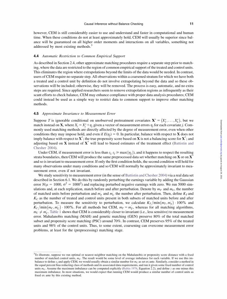
4.5 Approximate Invariance to Measurement Error

Suppose T is ignorable conditional on unobserved pretreatment covariates X� 5�X�1 ; . . . ;X

�k

�, but we

match instead on X, where Xj 5X�j 1gj given a vector of measurement errors gj for each covariate j. Com-

monly used matching methods are directly affected by the degree of measurement error, even when otherconditions they may impose hold, and even if E(gj) 5 0. In particular, balance with respect to X does notimply balance with respect to X*; the true propensity score based on X is not a balancing score for X*; andadjusting based on X instead of X* will lead to biased estimates of the treatment effect (Battistin andChesher 2004).

Under CEM, if measurement error is less than ej, ej > max(jgj,j), and it happens to respect the resultingstrata boundaries, then CEM will produce the same preprocessed data set whether matching on X or on X*

and so is invariant to measurement error. If only the first condition holds, the second condition will hold formany observations under many conditions and so CEM will normally be approximately invariant to mea-surement error, even if not invariant.

We study sensitivity to measurement error (in the sense of Battistin and Chesher 2004) via a real data setdescribed in Section 6.1. We do this by randomly perturbing the earnings variable by adding the Gaussianerror N(l 5 1000, r2 5 10002) and replacing perturbed negative earnings with zero. We run 5000 sim-ulations and, at each replication, match before and after perturbation. Denote by mT and mC, the numberof matched units before perturbation and m#

T and m#C the number after perturbation. Then, define KT and

KC as the number of treated and control units present in both subsets of matched units before and afterperturbation. To measure the sensitivity to perturbation, we calculate KT

�min

�mT ;m

#T

�� 100% and

KC

�min

�mC;m

#C

�� 100%. For all methods but CEM, mT 5m#

T , whereas for all matching algorithms,mC 6¼ m#

C. Table 1 shows that CEM is considerably closer to invariant (i.e., less sensitive) to measurementerror. Mahalanobis matching (MAH) and genetic matching (GEN) preserve 80% of the total matchedsubset and propensity score matching (PSC) around 70%. In contrast, CEM preserves 95% of the treatedunits and 98% of the control units. Thus, to some extent, coarsening can overcome measurement errorproblems, at least for the (preprocessing) matching stage.

3To illustrate, suppose we run optimal or nearest neighbor matching on the Mahalanobis or propensity score distance with a fixednumber of matched control units, mC. The result would be some level of average imbalance for each variable. If we use this im-balance to define ej and apply CEM, we would usually obtain a similar number for mC as set ex ante. Similarly, consider a method inthe equal percent bias reducting class of methods and its associated data requirements, and run it given some fixed number of controlunits mC. Assume the maximum imbalance can be computed explicitly (Rubin 1976, Equation 2.2), and define c as one minus thismaximum imbalance. In most situations, we would expect that running CEM would produce a similar number of control units asfixed ex ante by this existing method.




ownloaded from


4.6 Bounding Model Dependence

To make a causal inference, one must estimate the counterfactual potential outcome Yi(0) for each treatedunit (i.e, the value that Yi would take if Ti were 0 when it is in fact 1). To do this, we could use the value ofthe outcome variable for a different unit with a good match, say Yj, such that Xj � Yi. However, in the usualcase where insufficient exact matches exist, a better estimate might be obtained by a model, such as sometype of regression model: Y

�0�[m‘

�Xj

�, where Xj is the vector of covariates for the control units close to

treated i and m‘ð � Þ is one of many possible models. Model dependence is defined by how much m‘

�Xj

�varies as a function of the model m‘ for a given vector of covariates Xj (King and Zeng 2007). Unfor-tunately, in many situations, model dependence is remarkably large, so that apparently small and other-wise indefensible specification decisions in the regression can have large effects on causal estimates.

A key advantage of matching is that it should reduce model dependence. In other words, preprocessingdata via matching ought to lead to different modeling choices having considerably less influence on theestimate of the causal quantity of interest than it would without matching. This relationship has beenillustrated in real data by Ho et al. (2007), but it has never been proven mathematically for any previousmethod, EPBR or otherwise. In contrast, MIB methods have been shown to possess this property (Iacus,King, and Porro 2011), and since CEM is an MIB method, it too possesses this property.

In other words, by choosing the coarsening for each variable, a researcher also controls the bound on thedegree of model dependence possible. Less coarsening directly lowers the maximum possible level ofmodel dependence.

4.7 Bounding the Average Treatment Effect Estimation Error

Another attractive property of MIB matching methods, and one that distinguishes them from EPBR andother matching methods, is that their tuning parameters bound not only the model dependence used toestimate the causal effect but also the causal effect estimation error itself (from equation (3)). In particular,choosing CEM coarsening to be finer directly reduces the maximum possible estimation error.

To show this result for CEM, we first introduce a slight constraint on the possible range of functions g0(�)and then derive the theoretical bound. The following assumption restricts the sensitivity of g0(x1, . . ., xk)to changes in its arguments: along each direction (i.e., along each xj), g0 behaves like a Lipschitz function.We denote by N2j 5N1�N2� . . .�Nj21�Nj11� . . .�Nk, x2j 5 (x1,x2,. . .,xj21,xj11,. . .,xk), and g0(xjjx2j)5 g0(x1, x2, . . ., xk).

Assumption 1 (Lipschitz behavior).For each variable j (j 5 1, . . ., k), there exists a constant Lj, 0 < Lj <N, such that, for any values x#j 6¼ x$j

of xj,

maxx2j2N2j

��g0�x#j��x2j

�2g0

�x$j

��x2j

��<Ljdj�x#j; x$j

�;

where dj(�,�) is an appropriate distance for variable xj.This assumption is very mild and only bounds g0 from taking infinite values on finite sets. Given two

values x#j and x$j of the variable xj, the maximum excursion of g0, regardless of all possible values of theremaining variables xi (i 6¼ j), is bounded by the distance between x#j and x$j times some finite constant.This means that given finite variation in one variable, the function g0 does not explode. If this assumptiondoes not hold, g0 could have strange properties, such that even arbitrarily small and otherwise irrelevantimbalance in the covariates could produce arbitrarily large estimation error in the estimation of the treat-ment effect. This assumption easily fits essentially all functional forms used regularly in the socialsciences.

Table 1 Percentage of units present in matched sets both before and after perturbation, averaged over 5000simulations, and computational time (for all methods but CEM, KT 5 100%)

CEM (KT) CEM (KC) PSC (KC) MAH (KC) GEN (KC)

% Common units 95.3 97.7 70.2 80.9 80.0Seconds 0.07 0.07 0.08 0.15 126.64




ownloaded from


Without loss of generality, we measure distance for numerical covariates as dj(x, y) 5 jx 2 yj. Forcategorical variables, we adopt the following definitions for convenience, and without loss of generality.Let Xj be a categorical variable and H be the set of distinct values of Xj. Then, if H � U, where U is anabstract set of unordered categories, define the distance as d(x, y) 5 1{x 6¼ y}, where 1A 5 1 for elements inset A and 0 otherwise. If, alternatively, H � O, where O is the abstract set of ordered categories, thedistance is d(x, y) 5 jrank(x) 2 rank(y)j, where rank(x) is the rank/order of category x in H.

Then, the definitions in Section 2.7 imply directly that the estimation error, �E0 [ SATT2SATT^, isbounded from above and below by

��E0

��, that is, 2��E0

�� < SATT2��SATT^<

��E0

��and a consequence ofAssumption 1 is that jg0ðXiÞ2g0ðXiÞj<maxj5 1;...;kLjej. Therefore, for the CEM algorithm, which keepsmatched treated and control units for each covariate a maximum of ej apart, we conclude that��E0

��< maxj5 1;...;k

Ljej: ð7Þ

Thus, setting ej locally for each variable bounds the SATT estimation error, not merely the imbalancebetween treated and control groups. (We discuss how to estimate this in Section 5.5.2.).

4.8 The Number of Matched Units

If too many treated units are discarded, inferences with CEM may be inefficient. This can be remedied bywidening the degree of maximum imbalance. Of course, we might be concerned about the curse of di-mensionality, where the number of possible strata from the cross-tabulation of the possible values of X isordinarily huge. For example, suppose X is composed of 10,000 observations on 20 variables drawn fromindependent normal densities. Since 20-dimensional space is so large, no treated unit will likely be any-where near any control unit. In this situation, even very coarse bins under CEM will likely produce nomatches. For example, with only two bins for each variable, the 10,000 observations would need to besorted into more than a million strata. In data like these, no matching method could do any good.

Fortunately, most real data sets have much more highly correlated data than the independent draws inthe hypothetical example above, and so CEM, in practice, tends to produce reasonable numbers ofmatches. This has been our recurring experience in the numerous data sets we have analyzed withCEM. In addition, Iacus, King, and Porro (2011) show that if the number of control units is large enough,the number of cells with unmatched treated units goes to zero at a fixed and known rate. That is, in practice,if the data are useful for making causal inferences, CEM will normally produce a well-balanced data setwith a reasonable number of observations.

4.9 Computational Efficiency

An attractive feature of CEM is that it is extremely efficient computationally, especially compared to someother matching methods. Indeed, each observation i with vector of covariates Xi is stored as a recordcontaining only the coarsened values pasted one after the other in a single string. As a whole, for n ob-servations, we have only n strings stored. So, the number of covariates do not affect the dimension of thecoarsened data set (its length is always n) and finding observations in the same multidimensional cell hasthe same computational complexity of the tabulation of a distribution of n units (i.e., it is of order n). Thus,even if in principle one should search in the grid of an exponentially large number of cells, in practice, thesearch is only made on the nonempty cells, which are at most n. This is important because it means themethod works out-of-the-box on huge databases using SQL-type queries without the need for statisticalsoftware or modeling. In addition, the computational efficiency and simplicity of this CEM procedure aremuch easier to completely automate.

4.10 Empirical Properties

CEM has been compared to most commonly used methods in a large number of real data sets. Theseinclude analyses of Food and Drug Administration drug approval times (Carpenter 2002), job trainingprograms (Lalonde 1986), two large data sets evaluating disease management programs (King et al.




ownloaded from


2011), and the effects of having a daughter on a member of congress’ voting behavior (Washington 2008).We also extended our empirical experience by sampling from all social science causal analyses in progressin many fields by advertising help in making causal analyses in return for a look at researchers’ data,promising to preserve authors rights of first publication (Iacus, King, and Porro 2011). In almost all theseanalyses, CEM generated matched data sets with lower imbalance and a larger sample size than otherapproaches.

Finally, what may be the most commonly used method presently, propensity score matching, wasshown by King et al. (2011) to approximate random matching, thus increasing imbalance, in many circum-stances. CEM does not have this damaging property.

5 Extensions of CEM

CEM is so simple that it is easy to extend in a variety of productive ways. We offer seven extensions here.

5.1 Multicategory Treatments

Under CEM, we set e and then match the coarsened data, all without regard to the values of the treatmentvariable. This means that CEM works without modification for multicategory treatments: after the algo-rithm is applied, keep every stratum that contains all desired values of the treatment variable and discardthe rest. This is a simple approach that can be easily used with or in place of more complicated approaches,such as based on generalizations of the propensity score (Imbens 2000; Lu et al. 2001; Imai and van Dyk2004).

5.2 Combining CEM with Other Methods

CEM is one of the simplest methods with MIB properties (and the additional properties in Section 4) andso may have the widest applicability, but other improved methods could easily be developed for specificapplications by applying existing approaches within each CEM stratum. For example, instead of retainingall units matched within each stratum and moving to the analysis stage, we could fine-tune local (i.e.,sub-e) imbalance further by selecting or weighting units within each stratum via distance or other methods.Indeed, non-MIB methods can usually be made MIB if they operate within CEM strata, so long as thecoarsened strata take precedence in determining matches. Thus, full and optimal matching are not MIB,but if applied within CEM strata would be MIB and would inherit the properties given in Section 4.Genetic matching as defined in Diamond and Sekhon (2005) is not MIB, but by choosing a variable-by-variable caliper, it would be; if it were run within CEM strata, it would be MIB and would also meetthe congruence principle. Similarly, one could run the basic CEM algorithm and then use either a syntheticmatching approach (Abadie and Gardeazabal 2003), nonparametric adjustment (Abadie and Imbens2007), or weighted cross-validation (Galdo, Smith, and Black 2008) within each stratum and the MIBproperty would hold.

If the user does not know enough about X’s measurement to coarsen, then productive data analysis ofany kind may be infeasible. But in some applications, we can partition X into two sets, only the first ofwhich includes variables known to have an important effect on the outcome (such as in public health, age,sex, and a few diagnostic indicators). In this case, we may be willing to take good matches on any subset ofthe second set and to forgo the MIB property within this second set. To do this, we merely set e artificiallyhigh for this second set, but small as usual for the first set, and then apply a non-MIB method within CEMstrata. For example, because the relative importance of the variables is unknown, the propensity score orany other distance metric, if correctly specified, could be helpful. When the correct specification is un-likely, one can alternatively leave the remaining adjustment to the analysis stage, where analysts havemore experience assessing model fit.

5.3 Matching and Missing Data

When it comes to estimating causal effects in data with missing values, divergent messages areputting applied researchers in a difficult position. One message from methodologists writing on




ownloaded from


causal inference in observational data is that matching should be used to preprocess data prior tomodeling. Another message is that missing data should not be listwise deleted but should insteadbe treated via multiple imputation or another proper statistical approach (Rubin 1987; King et al.2001). Although most causal inference problems have some missing data, it is not obvious howto apply matching while properly dealing with missing data. Indeed, we know of no matching soft-ware that allows missing data for anything other than listwise deletion prior to matching, and nomissing data software that conducts or allows for matching. Thus, we now offer two options to usedboth in the same analysis enabled by CEM; all our software implementations of CEM allow for mul-tiply imputed data.

The simplest approach is to treat missing values as a discrete ‘‘observed’’ value and then to apply CEMwith other coarsening used for the nonmissing values. The default operation of our software uses thisapproach. In some situations, however, we might wish to customize this approach to the substance ofthe problem by coarsening the missing value with a specific observed value. For example, for surveyquestions on topics respondents may not be fully familiar with, the answers ‘‘no opinion’’ and ‘‘neutral’’may convey similar or in some cases identical information, and so grouping for the purpose of matchingmay be a reasonable approach. Since the original values of these variables would still be passed to theanalysis model, special procedures could still be utilized to distinguish between the effects of the twodistinct answers.

Although this first approach to missing data and matching will work for many applications, itwill be less useful when the occurrence of missing values are to some extent predictable from theobserved values of other variables in complicated ways we do not necessarily foresee and includein our customized coarsening operator. Indeed, this is precisely what the ‘‘missing at random’’assumption common in multiple imputation models is designed for. Thus, an alternative is to feedmultiply imputed data into a modified CEM algorithm. The modification works by first placingeach missing value in whichever coarsened stratum a plurality of the individual imputations falls.(Alternatively, at some expense in terms of complication, the imputations could stay in separatestrata and weights could be added.) Then, the rest of the algorithm works as usual. The key here isthat all the original uncoarsened variable values fed into CEM—in this case including the multipleuncoarsened imputed values for each missing value—are output from CEM as separately imputedmatched data sets. Then, as usual with multiple imputation, each imputed matched data set is analyzedseparately and the results combined. Thus, unlike with other matching procedures combined withimputation, multiple imputation followed by this modified CEM algorithm will produce proper un-certainty estimates.

5.4 Avoiding Consequences of Arbitrary Coarsenings

One seeming inconsistency with the basic CEM algorithm described in Section 3 is that it can be sensitiveto changes in X smaller than e near stratum boundaries even though it is insensitive to changes in X withinstrata. This point is irrelevant for CEM’s intended use, that is, when coarsening is chosen based on sub-stantive criteria (such as a college diploma marking a distinct point in an otherwise continuous educationvariable), but can be a concern if coarsening is set more arbitrarily or automatically. In this situation, allthe properties of CEM described in Section 4 still hold, but there may be an opportunity to increasethe matched sample size a bit more, given the same chosen balance level, even without relaxing anyassumptions.

In this situation, we run the basic CEM algorithm several times, each with a fixed value of e, andthus a fixed stratum size, but with values of the cutpoints shifted together by different amounts.(Our software implements this automatically.) We then use the single coarsening solution thatmaximizes the remaining sample size. The number of shifted coarsenings and the size of each maybe chosen by the user, but our default is to try only three since we find that the advantages of this procedureare small and additional improvements beyond this are not worth the computational time. Whicheverchoice the user makes, all the properties of the basic CEM method also apply to this slightly generalizedalgorithm.




ownloaded from


5.5 Automating User Choices

As described in Section 3, we recommend that users of CEM choose e based on their knowledge of thecovariate measurement process and other substantive criteria such as the likely importance of differentvariables. Although we have shown that making these decisions is relatively easy and intuitive in mostsituations, users may sometimes want an automated procedure to orient them or to make fast calculations.We offer several such approaches here.

5.5.1 Histogram bin size calculations

When automation is necessary because of the scale of the problem or to provide some orientation asa starting point, we note here that choosing e is very similar to the choice of the bin size in drawinghistograms. Some classic measures of bin size are based on the range of the data, an underlying normaldistribution, or the interquartile range. These are, respectively, known as Sturges,Dst 5 ðxn2x1Þ=ðlog2n11Þ, Scott, Dsc 5 3:5

ffiffiffiffi�s2n

pn21=3 (Scott 1992), and Freedman and Diaconis (1981)

Dfd 5 2�Q32Q1

�n21=3. More recently, Shimazaki and Shinomoto (2007) developed an approach based

on the Poisson sampling in time series analysis (in the attempt to recover spikes), which we find workswell. Our software offers these approaches as options.

5.5.2 Estimating the SATT error bound

Assumption 1 is a natural part of standard observational data analysis, but it gives no hint how big or smallthe Lj’s are. In practice, they can take any finite value, but their ranking implies a rough order on theimportance of each variable in affecting g0. That means that some insight about the size of ej inCEM and its effect on the treatment effect may come from information about Lj. Thus, we note thatLj, for variable j (j 5 1, . . ., k), may be estimated from the data as follows:

Lj 5 maxi1 6¼i22C

jYi1ð0Þ2Yi2ð0Þjdj�Xi1j;Xi2j

� : ð8Þ

These Lj are estimates from below of the true Lj’s, but they may still give insights about the relativeimportance of each variable on g0 for the given data. Under additional assumptions on g0, the estimators ofthe Lj may have better performance (e.g., g0 is linear or well approximated by a Taylor expansion). Equa-tion (7) is independent of the number of matched treated units mT when Lj are known, but, in general, the Lj

are not independent and can be estimated via equation (8). In such a case, the bound naturally depends onmT. Thus, although knowing that CEM bounds SATT error is an attractive property in and of itself, we cango further and estimate the value of this bound with E0 given as E0 5maxjLjej and use the terms Ljej asa hints during matching about which covariate may give rise to the largest estimation errors or bias inestimating SATT. Although equation (8) uses the outcome variable, it only does so for control units (as inHansen 2008), and so inducing selection bias is not a risk.

5.5.3 Inductive coarsening choices

Under CEM, setting balance by choosing e may yield too few observations in some applications. Ofcourse, this situation reveals a feature of the data, not a problem with the method, where the only realsolution is to collect more data. In some circumstances, however, this situation may cause users to rethinktheir choices for e and rerun CEM. Although we recommend that users make these choices based on thesubstance, we offer here an automated procedure that may help in understanding data problems, identifythe new types of data that would be most valuable to collect, or help them rethink their choices about e.

Thus, we now study systematic ways to relax a CEM solution (i.e., increase ej selectively) by usingh#5 ðh#1; . . . ; h#kÞ such that h# < h, that is, h#i 5 hi for all i but a subset of indexes j such that h#j<hj.When different relaxations or coarsenings, say h# and h$, lead to the same total numbers of matched units,mT(h#) 1 mC(h#) 5 mT(h$) 1 mC(h$), then an automated procedure needs a way to choose among thesesolutions that are for our purposes equivalent. We discriminate among these by minimizing the L1 dis-tance. Furthermore, although setting hj 5 1 is equivalent to dropping Xj from the match, we keep Xj with




ownloaded from


hj 5 1 to maintain comparability because the L1 distance depends on the number of covariates (as with anymeasure of dissimilarity in multidimensional histograms). In addition to keeping the number of covariatesthe same in this way, we also keep the bins of the multidimensional histogram used to calculate L1 thesame.

With these requirements, we adopt a heuristic algorithm, which we first describe conceptually,without regard to computer time, and then what we use in practice. Given the original user choiceof h, the algorithm relaxes each hj in increments of 2, that is, h#j 5 hj22, until h#j < 10 and then by 1or up to a user chosen minimally tolerable number of intervals, hmin

j . (We also shift each intermediatesolution as in Section 5.4.) We then repeat the procedure for pairs of variables, (hi, hj), triplets (hi, hj,hk), etc.4

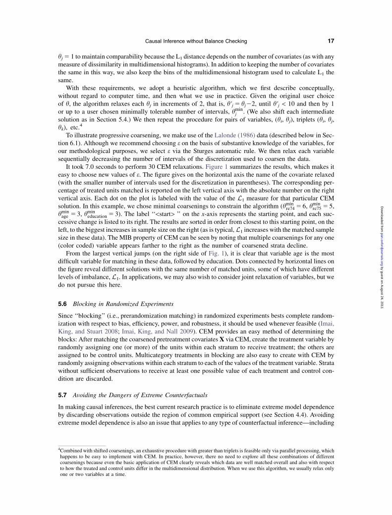
To illustrate progressive coarsening, we make use of the Lalonde (1986) data (described below in Sec-tion 6.1). Although we recommend choosing e on the basis of substantive knowledge of the variables, forour methodological purposes, we select e via the Sturges automatic rule. We then relax each variablesequentially decreasing the number of intervals of the discretization used to coarsen the data.

It took 7.0 seconds to perform 30 CEM relaxations. Figure 1 summarizes the results, which makes iteasy to choose new values of e. The figure gives on the horizontal axis the name of the covariate relaxed(with the smaller number of intervals used for the discretization in parentheses). The corresponding per-centage of treated units matched is reported on the left vertical axis with the absolute number on the rightvertical axis. Each dot on the plot is labeled with the value of the L1 measure for that particular CEMsolution. In this example, we chose minimal coarsenings to constrain the algorithm (hmin

re74 5 6, hminre75 5 5,

hminage 5 3, hmin

education 5 3). The label ‘‘<start> ’’ on the x-axis represents the starting point, and each suc-cessive change is listed to its right. The results are sorted in order from closest to this starting point, on theleft, to the biggest increases in sample size on the right (as is typical, L1 increases with the matched samplesize in these data). The MIB property of CEM can be seen by noting that multiple coarsenings for any one(color coded) variable appears farther to the right as the number of coarsened strata decline.

From the largest vertical jumps (on the right side of Fig. 1), it is clear that variable age is the mostdifficult variable for matching in these data, followed by education. Dots connected by horizontal lines onthe figure reveal different solutions with the same number of matched units, some of which have differentlevels of imbalance, L1. In applications, we may also wish to consider joint relaxation of variables, but wedo not pursue this here.

5.6 Blocking in Randomized Experiments

Since ‘‘blocking’’ (i.e., prerandomization matching) in randomized experiments bests complete random-ization with respect to bias, efficiency, power, and robustness, it should be used whenever feasible (Imai,King, and Stuart 2008; Imai, King, and Nall 2009). CEM provides an easy method of determining theblocks: After matching the coarsened pretreatment covariates X via CEM, create the treatment variable byrandomly assigning one (or more) of the units within each stratum to receive treatment; the others areassigned to be control units. Multicategory treatments in blocking are also easy to create with CEM byrandomly assigning observations within each stratum to each of the values of the treatment variable. Stratawithout sufficient observations to receive at least one possible value of each treatment and control con-dition are discarded.

5.7 Avoiding the Dangers of Extreme Counterfactuals

In making causal inferences, the best current research practice is to eliminate extreme model dependenceby discarding observations outside the region of common empirical support (see Section 4.4). Avoidingextreme model dependence is also an issue that applies to any type of counterfactual inference—including

4Combined with shifted coarsenings, an exhaustive procedure with greater than triplets is feasible only via parallel processing, whichhappens to be easy to implement with CEM. In practice, however, there no need to explore all these combinations of differentcoarsenings because even the basic application of CEM clearly reveals which data are well matched overall and also with respectto how the treated and control units differ in the multidimensional distribution. When we use this algorithm, we usually relax onlyone or two variables at a time.




ownloaded from


causal inferences, forecasts, and what if questions. Typically, scholars do this by eliminating data in theregion requiring extrapolation, outside the convex hull of the data (King and Zeng 2006). However, as iswidely recognized, the hull may contain voids with little data nearby where estimation would be modeldependent. Similarly, regions may exist just outside the hull, but near a lot of data just inside, for whicha small extrapolation may be safe.

CEM can help avoid these problems as follows. First, augment the covariate data set with a pseudo-observation that represents the values of X for the counterfactual inference of interest and then run CEMon the augmented data set. Observations that fall in the same stratum as the pseudoobservation can be usedto make a relatively model-free inference about this counterfactual point, and so the number of such ob-servations is a measure of the reliability of an inference about this counterfactual. This procedure rep-resents a small generalization (due to coarsening) of a point emphasized by Manski (1995), who would usee 5 0.

It may also be worth repeating this procedure after widening the definition of e to include the largestvalues you would be willing to extrapolate for your particular choice of dependent variable. For example,log mortality for most causes of death is known to vary relatively smoothly with age (Girosi and King2008), and so extrapolating age by 10 or 20 years would normally not be very model dependent, except forthe very young or very old. Thus, we might set eage in this way, even though it might normally be set muchsmaller for using the basic CEM algorithm where the goal would be to eliminate as much dependence onthese types of assumptions as possible. This additional procedure is of course more hazardous because itinvolves assumptions about a specific outcome variable and because of interactions. For example, even ifextrapolating age by 10 years is reasonable in one application, and extrapolating education by 4 years isalso reasonable, evaluating a counterfactual that involved simultaneously extrapolating 10 years of ageand 4 years of education beyond the data might well be unreasonable. Examples like these are much lesslikely to occur or matter if e is defined as we do for CEM.

6 CEM in Practice

We now offer an illustration of the operation of CEM based on simulations (Section 6.2) and real data(Section 6.3). We describe the data used in both sections first (Section 6.1).

6.1 Data

Data in this paper come from the National Supported Work Demonstration, a U.S. job training program(Lalonde 1986). The program provided training to the participants for 12–18 months and helped them infinding a job. The goal of the program was to increase participants’ earnings, and so 1978 earnings (re78) isthe key outcome variable. From this experiment, Lalonde (1986) created an experimental and an obser-vational data set for further analysis. A cleaned subset of both data sets created by Dehejia and Wahba(2002), which we also analyze, have been widely used in the matching literature as a benchmark forevaluating methods (e.g., Imbens 2003; Smith and Todd 2005). The experimental data set includes297 treated and 425 control units from the experiment, which, because of randomization, are easy tomatch. The observational data set combines the 297 treated units from the experiment with 2490 controlunits from an observational survey, the Panel Study of Income Dynamics. Lalonde et al. have shown thatone cannot recover SATT from the observational data set in part because the data are highly imbalancedand relatively few good matches exist within the control group. We use the experimental data set in Sec-tions 4.5 and 6.2 and the observational data set in Section 6.3.

Pretreatment variables in these data were measured for both participants and controls, and include age(age), years of education (education), marital status (married), lack of a high school diploma (nodegree),race (black and Hispanic), indicator variables for unemployment in 1974 (u74) and 1975 (u75), and realearnings in 1974 (re74) and 1975 (re75). Some of these are dichotomous (married, nodegree, black, His-panic, u74, and u75), some are categorical (age and education), and the earnings variables are continuousand highly skewed, with point masses at zero.




ownloaded from


6.2 Simulations

We now compare CEM to several other methods by using the data generation process chosen by Diamondand Sekhon (2005) to evaluate their algorithm. This involves using covariates chosen by Dehejia andWahba (1999), a subset of the Lalonde data, setting the (homogeneous) treatment effect to $1000,and generating Y via this highly nonlinear form:

Y5 1000 � T10:1 � expð0:7 � logðre7410:0110:7 � logðre7510:01ÞÞ1e

where e� N(0, 10). The value of the treatment variable is then assigned to each observation on the basis ofa true propensity score e, given by

ei 5 logit21n110:5 � l10:01 � age220:3 � education220:01 � logðre7410:01Þ210:01 � logðre7510:01Þ2

o;

where l is the linear predictor of the following misspecified logistic model used to estimate a propensityscore (as in Dehejia and Wahba 1999):

l5 111:428 � 1024 � age222:918 � 1023 � educ220:2275 � black20:8276 � hispanic10:2071 �married20:8232 � nodegree21:236 � 1029 � re742

15:865 � 10210 � re75220:04328 � u7420:3804 � u75

In each of 5000 replications from this process, we assign the treatment to observation i by samplingfrom the Bernoulli with parameter ei, that is, Ti � Bern (ei), so the number of prematch treated and controlunits in the sample varies over replications. We then compare SATT estimators based on the difference in

Table 2 Comparison of bias, standard deviation, root mean square error, computational speed (seconds), and the(1 measure of imbalance for the original data (RAW), Mahalanobis distance (MAH), propensity score matching (PSC),genetic matching (GEN), and CEM, with values averaged over 5000 Monte Carlo replications. Also given are the

number of treated and control units selected by each method

BIAS SD RMSE Treated Controls Seconds L1

RAW 2423.72 1566.49 1622.63 151 293 0.00 1.28MAH 784.80 737.93 1077.20 151 151 0.03 1.08PSC 260.45 1025.83 1058.28 151 151 0.02 1.23GEN 78.33 499.50 505.55 151 143 27.38 1.12CEM 0.78 111.39 111.38 86 151 0.03 0.76

Fig. 1 Relaxation of each covariate.




ownloaded from


means (RAW in Table 2), the nearest neighbor propensity score matching (PSC), the nearest neighborMahalanobis matching (MAH), genetic matching (GEN), and CEM using our automatically selecteddiscretization.

Following Diamond and Sekhon (2005), we report results in terms of the bias (BIAS), standard de-viation (SD), and root mean square error (RMSE) of the SATT estimate over the 5000 Monte Carlo rep-lications. We also report the average number of matched units, which is lower for CEM than for othermethods, given the automated coarsening we chose. In practice of course, coarsening should be chosenbased on the substance of the variables and so, in general, the number could be larger or smaller. Despitethis, CEM dominates the other methods on each of the three evaluative criteria. Table 2 also gives resultson computational speed and the L1 balance metric, which CEM also improves on.

Relative to the original data, Mahalanobis matching increases the absolute bias but reduces the var-iance, which nets out to reducing the RMSE by about a third. Propensity score matching reduces thevariance (but less than Mahalanobis) and also the bias, which nets to about the same RMSE. Geneticmatching reduces both bias and variance, resulting in about a two-thirds reduction in RMSE comparedto the raw data. In contrast, CEM eliminates 99.8% of the bias, and the vast majority of the variance, whichnets to a 93% reduction in RMSE as compared to the original data. CEM (programmed in R) is also about900 times faster than genetic matching (programmed mostly in C) and is feasible with many more co-variates and observations. Of course, each of these other methods have many potential uses, and the timingdifferences in particular do not matter much for smaller data sets, but at a minimum CEM would seem tobe very widely applicable.

We ran other Monte Carlo experiments with more difficult, complicated, and heterogeneous data gen-eration processes—and also allowed the different methods to estimate their own best estimand, keepingSATT constant, or letting it vary by also matching treated units—and reached similar conclusions. Kinget al. (2011) performed similar comparisons while also allowing PSM and MAH to work with calipers andshowed that CEM still dominates to some extent even more strongly than the results here. Even though thissection shows that CEM substantially outperforms other methods, it would be easy to outperform theseresults using other applications of CEM or the combined methods discussed in Section 5.2. The usual‘‘ping pong theorem’’ qualifications certainly apply.

6.3 Empirical Example

We now present a step-by-step illustration of estimating a causal effect in data from Lalonde (1986).

6.3.1 Matching

To begin a CEM analysis, we first choose a reasonable coarsening for each variable. The more coarseningwe allow, the more observations we will have, but larger the bound on model dependence and estimationerror. For education, we divide years of education in classes corresponding to different levels: grade school(0–6), middle school (7–8), high school (9–12), college (13–16), and graduate school (>16). For age, weuse standard labor force classes: (15–19), (20–24), (25–34), (35–44), (45–54), (55–64), and (>65) years.

The data includes two indicator variables to identify unemployment in 1974 and 1975 (u74 and u75); weinclude these or, since the unemployed have zero earnings, we instead equivalently add the interval [0, 1)

Table 3 Imbalance measured by difference in means between treated and control units on theoriginal data (RAW), after CEM, propensity score matching (PSM), PSM with re742 in the model (PSM*),

and CEM with five quantiles for re74 (CEM*)

Age Education re74 re75 u74 u75 Married Nodegree Black Hispanic

RAW 210.22 21.74 215,857.75 215,997.24 0.35 0.27 20.70 0.43 0.55 0.06PSM 23.55 20.34 23706.94 23243.38 0.21 0.15 20.31 0.16 0.10 0.01CEM 20.43 20.10 21158.83 21364.83 0.00 0.00 0.00 0.00 0.00 0.00

PSM* 23.96 20.31 23809.26 22959.22 0.20 0.13 20.31 0.15 0.11 0.02CEM* 20.44 20.13 21046.94 21140.66 0.00 0.00 0.00 0.00 20.00 0.00




ownloaded from


dollars to the coarsening of re74 and re75. We divide earnings into quantiles, calculated on the distribu-tions of positive earnings. The quantiles (25, 50, 75)% of re74 are (11,756, 18,925, 26,842). So finally, weobtain the following cutpoints for variable re74: [0–1), [1–11,756), [11,756–18,925), [18,925–26,842),and [26,842–137,149). For variable re75, we have [0–1), [1–11,069), [11,069–18,261), [18,261–26,855),and [26,855–156,653). The initial multidimensional imbalance is L1 5 0.977.

After running CEM with the above coarsening, we obtain mT 5 176 treated units matched with mC 5

218 control units, resulting in a multivariate imbalance of L1 5 0.806; this corresponds to a moderatelysized 17.47% imbalance reduction.

We now do a parallel analysis using the most common approach to propensity score matching. Thisinvolves using nearest neighbor matching on the estimated propensity score, where the score comes froma logistic regression using all pretreatment variables and all treated units matched. This produces a mul-tivariate imbalance of L1 5 0.953, which corresponds to a reduction of only 2.48% relative to the raw dataand considerably smaller than CEM’s result.

But what about the simpler univariate difference in means imbalance metric for which the propensityscore was designed? As can be seen in the first three rows of Table 3, or the triangles in Figure 2, propensityscore matching (PSM) reduces imbalance for each variable, but CEM reduces it more for every one.

In any matching method, the acceptable level of imbalance for a pretreatment variable depends on itsexpected effect on the outcome—with lower imbalance being more desirable for variables with largerexpected effects. Unfortunately, changing imbalance in predictable ways is often impossible with meth-ods, such as the propensity score, that use a scalar imbalance metric. The problem is complicated by thefact that the usual ways to assess model specification are irrelevant here; the only question is whetherimbalance is changed as predicted. For example, suppose we wish to reduce imbalance further forre74 and decide to try adding the term re742 to the propensity score logit model specification. The resultis that the in-sample fit (as measured by the AIC statistic) is improved, but row ‘‘PSM*’’ in Table 3, andthe ‘‘1’’ symbol in Figure 2, shows that imbalance on re74 has increased. Indeed, the direction of changein imbalance is unpredictable for the other variables as well, as can be seen, for example, in the reductionin imbalance for variable re75.

Consider how much easier tightening the imbalance is with CEM. We can, for example, change thecoarsening by splitting re74 into five quantiles instead of the previously used three. Row ‘‘CEM*’’ inTable 3, and the ‘‘�’’ symbol in Figure 2, shows that we vastly reduced the imbalance on this variableand others never exceed the maximum imbalance we specified ex ante. For example, although the im-balance slightly increases for age and education, this increase respects the MIB property: for ages, wetolerated a maximal imbalance of 5 years, so 0.01 increase of imbalance were deemed ex ante as irrelevant.Similarly for education.

One can improve propensity score matching by continuing to tweak and rerun the model, recheckimbalance, and rerun again, but because the imbalance results generally go in unpredictable directions,finding a specification that improves balance on all variables can often be challenging. In contrast, becauseit is a member of the MIB class of methods, CEM produce no surprises about imbalance, which makes dataanalysis far easier: reducing maximum imbalance on one variable never has any effect on the maximumimbalance specified for any of the other variables.

Fig. 2 Percentage of bias left after matching (relative to the RAW data at 100%), for CEM (n), CEM* (�), PSM*(1), and PSM (˚). This figure offers an alternative visualization of Table 3.




ownloaded from


6.3.2 Estimation

Finally, we illustrate ways of estimating the causal effect under CEM. We begin with the local SATT, usingthe CEM-matched units via linear regression using all variables in the data set. The result is an estimate ofsmT

521223:7 and leaves nT 2 mT 5 121 unmatched treated units. So one option is to extrapolate themodel estimated for the mT matched units to the remaining unmatched treated units to estimate SATT forall treated units. This approach yields snT 52$554:7, which is quite far from smT

.Another approach is to estimate the local SATT on the unmatched nT 2 mT 5 121 treated and control

nC 2 mC 5 2272 units only and then use formula 1 to obtain another estimate of the global SATT. Doingthis, we obtain snT2mT

521467:5 and thus another estimate of the global SATT:

snT 5176ð21223:7Þ1121ð21467:5Þ

297521323:1:

A somewhat more conservative approach in the extrapolation region of unmatched treated units is tofirst prune control units outside the hyperrectangle of the subsample of treated units. This approach leavesus with 121 treated units and 43 control units. In this case, we get snT2mT

# 52$7494:20 and

snT# 5121ð21223:7Þ1176ð27494:2Þ

297523778:4:

The differences in the estimates of the global SATT illustrate the unavoidable model dependence in theextrapolation region. For the local SATT, CEM enables one to produce a highly stable estimate that isrelatively invariant to the estimation method.

6.3.3 Defining the quantity of interest

In practice, most methods of matching select by treated and controls and so produce a definition of theestimand as part of the matching procedure. Since matching is a method of preprocessing, and so theestimand is defined prior to estimation, all the usual statistical properties, such as bias and efficiency,still apply. However, understanding what quantity (which ‘‘local SATT’’) is being estimated is crucial.Methodologists recognize this fact but rarely do anything about it. We offer here a simple way of definingthe estimand, via a parallel plot; see Figure 3. In a parallel plot, each observation in the original data set isrepresented by a single line that traces out its values on each of the continuous variables (horizontally)between its minimum and maximum values (vertically). We adapt this graphic for our purposes by col-oring matched units in blue and unmatched units in red. The estimand is the average treatment effect forthe people who were matched, which we can see from the figure are younger, have middling levels ofeducation, and receive lower earnings than the full group. This is the group for whom a relatively stable,not model dependent inference is available. Applications ought to use a parallel plot like this, or someother approach, to characterizing the quantity being estimated.

Fig. 3 Parallel plot of noncategorical variables for CEM matched units (blue) against unmatched units (red) in theLelonde versus Panel Study of Income Dynamics data.




ownloaded from


7 Concluding Remarks on What Can Go Wrong

We conclude here with a discussion of what can go wrong in applying CEM and how to avoid theseproblems.

Choosing the coarsening (setting e) appropriately is the primary issue to consider when running CEM.If an element of e is set too large, then information that might have been useful to produce better matchesmay be missed. This is an issue, but analysts have a second chance to avoid the consequences of thisproblem in the analysis after matching. Of course, the less precise the match, the more burden is puton getting the modeling assumptions correct in the analysis stage.

In contrast, if elements of e are set too small, then too many observations may be discarded withouta chance for compensation during the analysis stage. If they are set much too small, a solution may eitherbe unavailable or lead to a low-efficiency solution. One must also be careful allowing selection to occur onthe treated units and to recognize and clarify for readers the new estimand. As we use CEM in practice, wetend to choose higher standards for what constitutes a match and thus are sometimes left in real obser-vational data sets with fewer observations than we might have otherwise, with the result being less cova-riate imbalance, less model dependence, and less resulting statistical bias. In many cases, smaller CEMmatched data sets eliminate much heterogeneity, resulting also in causal estimates with smaller variances.With or without these lower variances, the additional bias reduction means that CEM-based estimates willnormally have lower mean square error as well. Of course, if e is set as high as you are comfortable with,and your matched data set is still too small, then no magical method will be able to fix this basic datainadequacy, and you will be left trying to model your way out of the problem or to collect more informativedata.

When used properly with informative data, CEM can reduce model dependence and bias and improveefficiency, across a wide range of potential applications. Even when it is possible to design a superiormatching method specially for a particular data set, the simplicity of CEM will ordinarily still be farbetter than the commonly used parametric-only approaches. In these situations, users may opt forCEM, but they should be aware of the potential gain from delving more deeply into the increasinglysophisticated methodological literature in this area.

Finally, all the issues with matching, in general, may also go wrong with CEM. For example, CEM willnot save you if an important covariate is not matched on, unless it is closely related to a variable that ismatched on.

References

Abadie, Alberto, and Javier Gardeazabal. 2003. The economic costs of conflict: A case study of the Basque Country. American

Economic Review 93:113–32.

Abadie, Alberto, and Guido W. Imbens. 2007. Bias-corrected matching estimators for average treatment effects. Unpublished man-

uscript. http://ksghome.harvard.edu/aabadie/research.html.

Austin, Peter C., and Muhammad M. Mamdani. 2006. A comparison of propensity score methods: A case-study estimating the

effectiveness of post-AMI statin use. Statistics in Medicine 25:2084–106.

Battistin, Erich, and Andrew Chesher. 2004. The impact of measurement error on evaluation methods based on strong ignorability .

Working paper, Institute for Fiscal Studies, London.

Carpenter, Daniel Paul. 2002. Groups, the media, agency waiting costs, and FDA drug approval. American Journal of Political

Science 46:490–505.

Cochran, William G., and Donald B. Rubin. 1973. Controlling bias in observational studies: A review. Sankhya: The Indian Journal of

Statistics, Series A 35, Part 4:417–66.

Crump, Richard K., V. Joseph Hotz, Guido W. Imbens, and Oscar Mitnik. 2009. Dealing with limited overlap in estimation of average

treatment effects. Biometrika 96:187.

Dehejia, Rajeev H., and Sadek Wahba. 1999. Causal effects in nonexperimental studies: Re-evaluating the evaluation of training

programs. Journal of the American Statistical Association 94:1053–62.

———. 2002. Propensity score matching methods for non-experimental causal studies. Review of Economics and Statistics

84:151–61.

Diamond, Alexis, and Jasjeet Sekhon. 2005. Genetic matching for estimating causal effects: A new method of achieving balance in

observational studies. Working paper, http://jsekhon.fas.harvard.edu/ (accessed 2005).

Freedman, David, and Persi Diaconis. 1981. On the histogram as a density estimator: L2 theory. Probability Theory and Related Fields

57:453–76.

Galdo, Jose, Jeffrey Smith, and Dan Black. 2008. Bandwidth selection and the estimation of treatment effects with unbalanced data.

Working paper, University of Michigan.




ownloaded from


Girosi, Federico, and Gary King. 2008. Demographic forecasting. Princeton, NJ: Princeton University Press. Unpublished manu-

script. http://gking.harvard.edu/files/smooth/ (accessed 2008).

Hansen, Ben. 2008. The prognostic analogy of the propensity score. Biometrika 95:481–88.

Heckman, James, H. Ichimura, and P. Todd. 1997. Matching as an econometric evaluation estimator: Evidence from evaluating a job

training program. Review of Economic Studies 64:605–54.

Ho, Daniel, Kosuke Imai, Gary King, and Elizabeth Stuart. 2007. Matching as nonparametric preprocessing for reducing model

dependence in parametric causal inference. Political Analysis 15:199–236. http://gking.harvard.edu/files/abs/matchp-abs.shtml

(accessed 2007).

Iacus, Stefano M., Gary King, and Giuseppe Porro. 2009. CEM: Coarsened Exact Matching Software. Journal of Statistical Software

30(9), http://gking.harvard.edu/cem.

———. 2011. Multivariate matching methods that are Monotonic Imbalance Bounding. Journal of the American Statistical Asso-

ciation. http://gking.harvard.edu/files/abs/cem-math-abs.shtml.

———. 2011b. Replication data for: Causal inference without balance checking: Coarsened Exact Matching. Murray Research

Archive [distributor] V1 [version]. http://hdl.handle.net/1902.1/15601.

Iacus, Stefano M., and Giuseppe Porro. 2007. Missing data imputation, matching and other applications of random recursive par-

titioning. Computational Statistics and Data Analysis 52:773–89.

———. 2008. Invariant and metric free proximities for data matching: An R package. Journal of Statistical Software 25(11):1–22.

———. 2009. Random recursive partitioning: A matching method for the estimation of the average treatment effect. Journal of

Applied Econometrics 24:163–85.

Imai, Kosuke, Gary King, and Clayton Nall. 2009. The essential role of pair matching in cluster-randomized experiments, with

application to the Mexican universal health insurance evaluation. Statistical Science 24(1):29–53. http://gking.harvard.edu/

files/abs/cluster-abs.shtml.

Imai, Kosuke, Gary King, and Elizabeth Stuart. 2008. Misunderstandings among experimentalists and observationalists about causal

inference. Journal of the Royal Statistical Society, Series A 171, 2:481–502. http://gking.harvard.edu/files/abs/matchse-abs.shtml

(accessed 2008).

Imai, Kosuke, and D. A. van Dyk. 2004. Causal inference with general treatment regimes: Generalizing the propensity score. Journal

of the American Statistical Association 99:854–66.

Imbens, Guido W. 2000. The role of the propensity score in estimating dose-response functions. Biometrika 87:706–10.

———. 2003. Sensitivity to exogeneity assumptions in program evaluation. American Economic Review 96:126–32.

———. 2004. Nonparametric estimation of average treatment effects under exogeneity: A review. Review of Economics and

Statistics 86:4–29.

Imbens, Guido W., and Joshua D. Angrist. 1994. Identification and estimation of local average treatment effects. Econometrica

62:467–75.

King, Gary, James Honaker, Anne Joseph, and Kenneth Scheve. 2001. Analyzing incomplete political science data: An alternative

algorithm for multiple imputation. American Political Science Review 95:49–69. http://gking.harvard.edu/files/abs/evil-abs.shtml

(accessed 2001).

King, Gary, Richard Nielsen, Carter Coberley, James Pope, and Aaron Wells. 2011. Comparative effectiveness of matching methods

for causal inference.

King, Gary, and Langche Zeng. 2006. The dangers of extreme counterfactuals. Political Analysis 14:131–59. http://gking.

harvard.edu/files/abs/counterft-abs.shtml.

———. 2007. When can history be our guide? The pitfalls of counterfactual inference. International Studies Quarterly 51:183–210.

http://gking.harvard.edu/files/abs/counterf-abs.shtml.

Lalonde, Robert. 1986. Evaluating the econometric evaluations of training programs. American Economic Review 76:604–20.

Lu, Bo, Elaine Zanuto, Robert Hornik, and Paul R. Rosenbaum. 2001. Matching with doses in an observational study of a media

campaign against drug abuse. Journal of the American Statistical Association 96:1245–53.

Manski, Charles F. 1995. Identification problems in the social sciences. Cambridge, MA: Harvard University Press.

Mielke, Paul W., and Kenneth J. Berry. 2007. Permutation methods: A distance function approach. New York: Springer.

Morgan, Stephen L., and Christopher Winship. 2007. Counterfactuals and causal inference: Methods and principles for social

research. Cambridge: Cambridge University Press.

Rosenbaum, Paul R., Richard N. Ross, and Jeffrey H. Silber. 2007. Minimum distance matched sampling with fine balance in an

observational study of treatment for ovarian cancer. Journal of the American Statistical Association 102:75–83.

Rubin, Donald B. 1976. Inference and missing data. Biometrika 63:581–92.

———. 1987. Multiple imputation for nonresponse in surveys. New York: John Wiley.

———. 2001. Using propensity scores to help design observational studies: Application to the tobacco litigation. Health Services &

Outcomes Research Methodology 2:169–88.

———. 2006. Matched sampling for causal effects. Cambridge, UK: Cambridge University Press.

Scott, David W. 1992. Multivariate density estimation. Theory, practice and visualization. New York: John Wiley & Sons, Inc.

Shimazaki, Hideaki, and Shigeru Shinomoto. 2007. A method for selecting the bin size of a time histogram. Neural Computation

19:1503–27.

Smith, Jeffrey A., and Petra E. Todd. 2005. Does matching overcome LaLonde’s critique of nonexperimental estimators? Journal of

Econometrics 125:305–53.

Washington, Ebonya L. 2008. Female socialization: How daughters affect their legislator fathers’ voting on woman’s issues.

American Economic Review 98:311–32.




ownloaded from


causal inference without balance checking: coarsened exact ...causal inference without balance...

Documents