cem: coarsened exact matching in stata - gary king · of cem is to temporarily coarsen each...
TRANSCRIPT

The Stata Journal (2009)9, Number 4, pp. 524–546
cem: Coarsened exact matching in Stata
Matthew BlackwellHarvard University
Cambridge, MA
Stefano IacusUniversita degli Studi di Milano
Milano, [email protected]
Gary KingHarvard University
Cambridge, MA
Giuseppe PorroUniversita degli Studi di Trieste
Trieste, [email protected]
Abstract. In this article, we introduce a Stata implementation of coarsened exactmatching, a new method for improving the estimation of causal effects by reduc-ing imbalance in covariates between treated and control groups. Coarsened exactmatching is faster, is easier to use and understand, requires fewer assumptions,is more easily automated, and possesses more attractive statistical properties formany applications than do existing matching methods. In coarsened exact match-ing, users temporarily coarsen their data, exact match on these coarsened data,and then run their analysis on the uncoarsened, matched data. Coarsened exactmatching bounds the degree of model dependence and causal effect estimation er-ror by ex ante user choice, is monotonic imbalance bounding (so that reducing themaximum imbalance on one variable has no effect on others), does not require aseparate procedure to restrict data to common support, meets the congruence prin-ciple, is approximately invariant to measurement error, balances all nonlinearitiesand interactions in sample (i.e., not merely in expectation), and works with mul-tiply imputed datasets. Other matching methods inherit many of the coarsenedexact matching method’s properties when applied to further match data prepro-cessed by coarsened exact matching. The cem command implements the coarsenedexact matching algorithm in Stata.
Keywords: st0176, cem, imbalance, matching, coarsened exact matching, causalinference, balance, multiple imputation
1 Introduction
The cem command is designed to improve the estimation of causal effects via a powerfulmethod of matching that is widely applicable in observational data, and easy to under-stand and use (if you understand how to draw a histogram, you will understand thismethod). The command implements the coarsened exact matching (CEM) algorithmdescribed in Iacus, King, and Porro (2008).
CEM is a monotonic imbalance-reducing matching method, which means that thebalance between the treated and the control groups is chosen by ex ante user choicerather than being discovered through the usual laborious process of checking after thefact, tweaking the method, and repeatedly reestimating. CEM also assures that adjust-
c© 2009 StataCorp LP st0176

M. Blackwell, S. Iacus, G. King, and G. Porro 525
ing the imbalance on one variable has no effect on the maximum imbalance of any other.CEM strictly bounds through ex ante user choice both the degree of model dependenceand the average treatment-effect estimation error, eliminates the need for a separateprocedure to restrict data to common empirical support, meets the congruence princi-ple, is robust to measurement error, works well with multiple-imputation methods formissing data, can be completely automated, and is extremely fast computationally, evenwith very large datasets. After preprocessing data with CEM, the analyst may then usea simple difference in means or whatever statistical model he or she would have appliedwithout matching.
CEM can also be used to improve other methods of matching by applying thosemethods to CEM-matched data (they formally inherit CEM’s properties if applied withinCEM strata). CEM also works well for determining blocks in randomized experimentsand evaluating extreme counterfactuals.
2 Background
2.1 Notation
Consider a sample of n units randomly drawn from a population of N units, wheren ≤ N . For unit i, denote Ti as an indicator variable with the value Ti = 1 if unit ireceives the treatment (and so is a member of the “treated” group) and the value Ti = 0if it does not (and is therefore a member of the “control” group). The outcome variableis denoted Y, where Yi(0) is the potential outcome for observation i if the unit doesnot receive treatment and Yi(1) is the potential outcome if the (same) unit does receivetreatment. For each observed unit, the observed outcome is Yi = TiYi(1)+(1−Ti)Yi(0),and so Yi(0) is unobserved if i receives treatment and Yi(1) is unobserved if i does notreceive treatment.
To compensate for the observational data problem where the treated and the controlgroups are not necessarily identical before treatment (and, lacking random assignment,not the same on average), matching estimators attempt to control for pretreatment co-variates. For this purpose, we denote X = (X1,X2, . . . , Xk) as a k-dimensional dataset,where each Xj is a column vector of observed values of pretreatment variable j for then sample observations (possibly drawn from a population of size N). That is, X = Xij ,i = 1, . . . , n and j = 1, . . . , k.
2.2 Quantities of interest
As usual, the treatment effect (TE) for unit i, TEi = Yi(1) − Yi(0), is unobserved. Allrelevant causal quantities of interest are functions of TEi, for different groups of units,and so must be estimated. We focus on the sample average treatment effect on thetreated (SATT):
SATT =1
nT
∑i∈T
TEi (1)

526 Coarsened exact matching
where nT =∑n
i=1 Ti and T = (1 ≤ i ≤ n : Ti = 1). Matching algorithms sometimes alsochange the quantity being estimated to one that can be estimated without much modeldependence by selecting control or treated units.
We assume that treatment assignment is ignorable conditional on X. This assump-tion is often stated as “no unmeasured confounders” or “no omitted variables”. For-mally, this means that the treatment assignment is independent of the potential out-comes:
P {T |X,Y (0), Y (1)} = P (T |X) (2)
2.3 Existing matching methods and practice
Matching is a nonparametric method of controlling for some of or all the confound-ing influence of pretreatment control variables in observational data. The key goal ofmatching is to prune observations from the data so that the remaining data have bet-ter balance between the treated and the control groups, meaning that the empiricaldistributions of the covariates (X) in the groups are more similar. Exactly balanceddata means that controlling further for X is unnecessary (because it is unrelated tothe treatment variable), and so a simple difference in means on the matched data canestimate the causal effect; approximately balanced data require controlling for X witha model (such as the same model that would have been used without matching), butthe only inferences necessary are those relatively close to the data, leading to less modeldependence and reduced statistical bias than without matching.
The most common matching methods involve finding, for each treated unit, at leastone control unit that is “similar” on the covariates. The distinction between methods ishow to define this similarity. For example, exact matching simply matches a treated unitto all the control units with the same covariate values. Unfortunately, because of therichness of covariates in many examples, this method often produces very few matches.A whole host of approximate matching methods specify a metric to find control unitsthat are close to the treated unit. This metric is often the Mahalanobis distance or thepropensity score (which is simply the probability of being treated, conditional on thecovariates). Many of these related methods are implemented in Stata (Becker and Ichino2002; Abadie et al. 2004; Leuven and Sianesi 2003; Abadie, Diamond, and Hainmuellerforthcoming-a, -b). A problem with this type of solution is that it requires the user toset the size of the matching solution ex ante, and then check for balance ex post. Thusanalysts must check for balance after the algorithm is finished, and then respecify amatching model and recheck balance, etc. This process repeats until the user obtainsan acceptable amount of balance.
Because matching is simply a data-preprocessing technique, analysts must still applystatistical estimators to the data after matching. When one-to-one exact matching isused, a simple difference in means between Y in the treated group and the control groupprovides an estimator of the causal effect. When the match is not exact, a parametricmodel must be used to control for the differences in the covariates across the treated andthe control groups. This may be a linear regression, a maximum likelihood estimator,

M. Blackwell, S. Iacus, G. King, and G. Porro 527
or some other estimator. Applying a matching method to the data before analysis canreduce the degree of model dependence (Ho et al. 2007).
One wrinkle in the analysis of matched data occurs when there are not equal numbersof treated and control units within strata. In this situation, estimators require weightingobservations according to the size of their strata (Iacus, King, and Porro 2008).
3 CEM
3.1 The algorithm
The central motivation for CEM is that while exact matching provides perfect balance, ittypically produces few matches because of curse-of-dimensionality issues. For instance,adding one continuous variable to a dataset effectively kills exact matching because twoobservations are unlikely to have identical values on a continuous measure. The ideaof CEM is to temporarily coarsen each variable into substantively meaningful groups,exact match on these coarsened data, and then retain only the original (uncoarsened)values of the matched data.
Because coarsening is a process at the heart of measurement, many analysts knowhow to coarsen a variable into groups that preserve information. For instance, educationmay be measured in years, but many would be comfortable grouping observations intocategories of high school, some college, college graduates, etc. This method works byexact matching on distilled information in the covariates as chosen by the user.
The algorithm works as follows:
1. Begin with the covariates X and make a copy, which we denote as X∗.
2. Coarsen X∗ according to user-defined cutpoints or CEM’s automatic binning al-gorithm.
3. Create one stratum per unique observation of X∗, and place each observation ina stratum.
4. Assign these strata to the original data, X, and drop any observation whosestratum does not contain at least one treated and one control unit.
Once completed, these strata are the foundations for calculating the treatment effect.The inherent tradeoff of matching is reflected in CEM, too: larger bins (more coarsening)used to make X∗ will result in fewer strata. Fewer strata will result in more diverseobservations within the same strata and, thus, higher imbalance.
It is important that CEM prunes both treated and control units. This process changesthe quantity of interest under study to the treatment effect in the post matching sub-sample. This change is reasonable so long as the decision is transparent (see, e.g.,Crump et al. [2009]).

528 Coarsened exact matching
3.2 The benefits
Iacus, King, and Porro (2008) derive many of the properties of the CEM algorithm andwe review some of them here. The key property of CEM is that it is in a class of match-ing methods called monotonic imbalance bounding. Monotonic imbalance boundingmethods bound the maximum imbalance in some feature of the empirical distributionsthrough an ex ante choice by the user. In CEM, this ex ante choice is the coarsening.As the coarsening on any variable becomes finer (the bins become more narrow), thebound on the maximum imbalance on the moments of that variable becomes tighter.This is also true for the bound on differences in the empirical quantiles. Furthermore,this choice also bounds the maximum imbalance on the full multivariate histogram oftreated and control units, which includes all interactions and nonlinearities. By choos-ing the coarsening ex ante, users can control the amount of imbalance in the matchingsolution. Iacus, King, and Porro (2008) also show that CEM bounds both the error inestimating the average treatment effect and the amount of model dependence.
Aside from bounding the imbalance between the treated and control groups, CEM
has a number of other beneficial properties. First, CEM meets the congruence principle,which states that the data space and analysis space should be the same. Methods thatfail to meet this principle often produce strange or counterintuitive results. Methodsthat meet the principle allow analysts to leverage their substantive knowledge of thedata to find better matches. Second, CEM automatically restricts the matched datato areas of common empirical support. This is necessary to remove the possibility ofdifficult-to-justify extrapolations of the causal effect that end up being heavily modeldependent (King and Zeng 2006). Finally, CEM is computationally very efficient, evenfor large datasets.
4 An extended example
We show here how to use cem1 through a simple running example: the national sup-ported work demonstration data, also known as the LaLonde dataset (LaLonde 1986).In this dataset, training was provided to selected individuals for 12–18 months, as washelp finding a job in the hopes of increasing the participant’s earnings. The treatmentvariable, treated, is 1 for participants (the treatment group) and 0 for nonparticipants(the control group). The key outcome variable is earnings in 1978 (re78). The statisticalgoal is to estimate a specific version of a causal effect: the SATT.
Because participation in the command was not assigned strictly at random, we mustcontrol for a set of pretreatment variables by the CEM algorithm. These pretreatment
1. cem is licensed under GNU General Public License (GLP2). For more information, seehttp://gking.harvard.edu/cem/. To install cem in Stata 10 or later, type
. net from http://gking.harvard.edu/cem/
. net install cem
In addition to the Stata version of cem, there is an R version in the cem package. The examplepresented here is also used in that package as a vignette and includes some obvious overlap in prose.
M. Blackwell, S. Iacus, G. King, and G. Porro 529
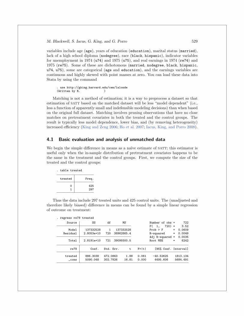
variables include age (age), years of education (education), marital status (married),lack of a high school diploma (nodegree), race (black, hispanic), indicator variablesfor unemployment in 1974 (u74) and 1975 (u75), and real earnings in 1974 (re74) and1975 (re75). Some of these are dichotomous (married, nodegree, black, hispanic,u74, u75), some are categorical (age and education), and the earnings variables arecontinuous and highly skewed with point masses at zero. You can load these data intoStata by using the command
. use http://gking.harvard.edu/cem/lalonde(Written by R. )
Matching is not a method of estimation; it is a way to preprocess a dataset so thatestimation of SATT based on the matched dataset will be less “model dependent” (i.e.,less a function of apparently small and indefensible modeling decisions) than when basedon the original full dataset. Matching involves pruning observations that have no closematches on pretreatment covariates in both the treated and the control groups. Theresult is typically less model dependence, lower bias, and (by removing heterogeneity)increased efficiency (King and Zeng 2006; Ho et al. 2007; Iacus, King, and Porro 2008).
4.1 Basic evaluation and analysis of unmatched data
We begin the simple difference in means as a naıve estimate of SATT; this estimator isuseful only when the in-sample distribution of pretreatment covariates happens to bethe same in the treatment and the control groups. First, we compute the size of thetreated and the control groups:
. table treated
treated Freq.
0 4251 297
Thus the data include 297 treated units and 425 control units. The (unadjusted andtherefore likely biased) difference in means can be found by a simple linear regressionof outcome on treatment:
. regress re78 treated
Source SS df MS Number of obs = 722F( 1, 720) = 3.52
Model 137332528 1 137332528 Prob > F = 0.0609Residual 2.8053e+10 720 38962865.4 R-squared = 0.0049
Adj R-squared = 0.0035Total 2.8191e+10 721 39099300.5 Root MSE = 6242
re78 Coef. Std. Err. t P>|t| [95% Conf. Interval]
treated 886.3038 472.0863 1.88 0.061 -40.52625 1813.134_cons 5090.048 302.7826 16.81 0.000 4495.606 5684.491

530 Coarsened exact matching
Thus our estimate of SATT is 886.3. Because the variable treated was not ran-domly assigned, the pretreatment covariates differ between the treated and the controlgroups. To see this, we focus on these pretreatment covariates: age, education, black,nodegree, and re74.
The overall imbalance is given by the L1 statistic, introduced in Iacus, King, andPorro (2008) as a comprehensive measure of global imbalance. It is based on the L1
difference between the multidimensional histogram of all pretreatment covariates in thetreated group and the same in the control group. First, we coarsen the covariates intobins. To use this measure, we require a list of bin sizes for the numerical variables. Ourfunctions compute these automatically, or they can be set by the user.2 Then we cross-tabulate the discretized variables as X1×· · ·×Xk for the treated and the control groupsseparately, and record the k-dimensional relative frequencies for the treated f�1···�k
andfor the control g�1···�k
units. Finally, our measure of imbalance is the absolute differenceover all the cell values:
L1(f, g) =12
∑�1···�k
| f�1···�k− g�1···�k
| (3)
Perfect global balance (up to coarsening) is indicated by L1 = 0, and larger valuesindicate larger imbalance between the groups, with a maximum of L1 = 1, which indi-cates complete separation. If we denote the relative frequencies of a matched datasetby fm and gm, then a good matching solution would produce a reduction in the L1
statistic; that is, we would hope to have L1(fm, gm) ≤ L1(f, g).
We compute the L1 statistic, as well as several unidimensional measures of imbal-ance, via our imbalance command. In our running example,
. imbalance age education black nodegree re74, treatment(treated)
Multivariate L1 distance: .50759358
Univariate imbalance:
L1 mean min 25% 50% 75% maxage .10119 .1792 0 1 0 -1 -6
education .10047 .19224 1 0 1 1 2black .00135 .00135 0 0 0 0 0
nodegree .08348 -.08348 0 -1 0 0 0re74 .0522 -101.49 0 0 69.731 584.92 -2139
2. Of course, as with drawing histograms, the choice of bins affects the final result. The crucial pointis to choose one and keep it the same throughout to allow for fair comparisons. The particularchoice is less crucial.

M. Blackwell, S. Iacus, G. King, and G. Porro 531
Only the overall L1 statistic measure includes imbalance with respect to the full jointdistribution, including all interactions, of the covariates; for our example, L1 = 0.5076.The L1 value is not valuable on its own, but rather as a point of comparison betweenmatching solutions. The value 0.5076 is a baseline reference for the unmatched data.Once we have a matching solution, we will compare its L1 value to 0.5076 and gauge theincrease in balance due to the matching solution from that difference. Thus L1 worksfor imbalance as R2 works for model fit: the absolute values mean less than comparisonsbetween matching solutions. The unidimensional measures in the table are all computedfor each variable separately.
The first column, labeled L1, reports the Lj1 measure, which is L1 computed for
the jth variable separately (which of course does not include interactions). The secondcolumn in the table of unidimensional measures, labeled mean, reports the differencein means. The remaining columns in the table report the difference in the empiricalquantiles of the distributions of the two groups for the 0th (min), 25th, 50th, 75th, and100th (max) percentiles for each variable.
This particular table shows that variable re74 is imbalanced in the raw data inmany ways and variable age is balanced in means but not in the quantiles of the twodistributions. This table also illustrates the point that balancing only the means betweenthe treated and the control groups does not necessarily guarantee balance in the rest ofthe distribution. Most important, of course, is the overall L1 measure, because even ifthe marginal distribution of every variable is perfectly balanced, the joint distributioncan still be highly imbalanced.
4.2 CEM algorithm
We now apply the CEM algorithm by calling the cem command. The CEM algorithmperforms exact matching on coarsened data to determine matches and then passes onthe uncoarsened data from observations that were matched to estimate the causal effect.Exact matching works by first sorting all the observations into strata, each of which hasidentical values for all the coarsened pretreatment covariates, and then discarding allobservations within any stratum that does not have at least one observation for eachunique value of the treatment variable.
To run this algorithm, we must choose a type of coarsening for each covariate. Weshow how this is done via a fully automated procedure in the next section. Then weshow how to use explicit prior knowledge to choose the coarsening, which is normallypreferable when feasible.
(Continued on next page)

532 Coarsened exact matching
In CEM, the treatment variable may be dichotomous or multichotomous. Alterna-tively, cem may be used for randomized block experiments without specifying a treat-ment variable; here the strata are simply returned without any pruning of observations.
Automated coarsening
In our running example, we have a dichotomous treatment variable. In the follow-ing code, we match on our chosen pretreatment variables, but not re78, which is theoutcome variable and so should never be included.
The output contains useful information about the match, including a (small) tableabout the number of observations in total, matched, and unmatched by treatment group,as well as the results of a call to the imbalance command for information about thequality of the matched data. Because cem bounds the imbalance ex ante, the mostimportant information is the number of observations matched. But the results alsogive the imbalance in the matched data by using the same measures as described insection 4.1 on the original data. Thus
. cem age education black nodegree re74, treatment(treated)
Matching Summary:-----------------Number of strata: 205Number of matched strata: 67
0 1All 425 297
Matched 324 228Unmatched 101 69
Multivariate L1 distance: .46113967
Univariate imbalance:
L1 mean min 25% 50% 75% maxage .13641 -.17634 0 0 0 0 -1
education .00687 .00687 1 0 0 0 0black 3.2e-16 -2.2e-16 0 0 0 0 0
nodegree 5.8e-16 4.4e-16 0 0 0 0 0re74 .06787 34.438 0 0 492.23 39.425 96.881
We can see from these results the number of observations matched and thus retained,as well as those that were pruned because they were not comparable. By comparingthe imbalance results with the original imbalance table given in the previous section,we can see that a good match can produce a substantial reduction in imbalance, notonly in the means, but also in the marginal and joint distributions of the data.
The cem command also generates weights (stored in cem weights) for use in theevaluation of imbalance measures and estimates of the causal effect.

M. Blackwell, S. Iacus, G. King, and G. Porro 533
Coarsening by explicit user choice
The power and simplicity of cem comes from choosing the coarsening yourself ratherthan using the automated algorithm as in the previous section. Choosing the coarseningenables you to set the maximum level of imbalance ex ante, which is a direct functionof the coarsening you choose. By controlling the coarsening, you also put an explicitbound on the degree of model dependence and the SATT estimation error.
Fortunately, the coarsening is a fundamentally substantive act, almost synonymouswith the measurement of the original variables. If you know something about the datayou are analyzing, you almost surely have enough information to choose the coarsening.(And if you do not know something about the data, you might ask why you are analyzingit in the first place!)
In general, we want to set the coarsening for each variable such that substantivelyindistinguishable values are grouped and assigned the same numerical value. Groupsmay be of different sizes if appropriate. Recall that any coarsening during cem is usedonly for matching; the original values of the variables are passed on to the analysis stagefor all matched observations.
For numerical variables, we can use the cutpoints syntax in cem. Thus, for exam-ple, in the U.S. educational system, the following discretization of years of educationcorresponds to different levels of school:
Grade school 0–6Middle school 7–8High school 9–12College 13–16Graduate school >16
Using these natural breaks in the data to create the coarsening is generally a goodapproach and certainly better than using fixed bin sizes (as in caliper matching) thatdisregard these meaningful breaks. In our data, no respondents fall in the last category,
(Continued on next page)
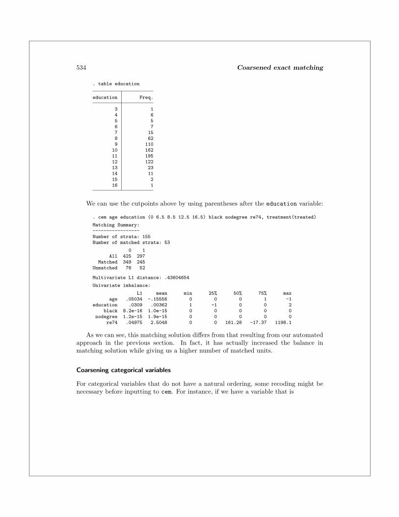
534 Coarsened exact matching
. table education
education Freq.
3 14 65 56 77 158 629 11010 16211 19512 12213 2314 1115 216 1
We can use the cutpoints above by using parentheses after the education variable:
. cem age education (0 6.5 8.5 12.5 16.5) black nodegree re74, treatment(treated)
Matching Summary:-----------------Number of strata: 155Number of matched strata: 53
0 1All 425 297
Matched 349 245Unmatched 76 52
Multivariate L1 distance: .43604654
Univariate imbalance:
L1 mean min 25% 50% 75% maxage .05034 -.15556 0 0 0 1 -1
education .0309 .00362 1 -1 0 0 2black 8.2e-16 1.0e-15 0 0 0 0 0
nodegree 1.2e-15 1.9e-15 0 0 0 0 0re74 .04975 2.5048 0 0 161.28 -17.37 1198.1
As we can see, this matching solution differs from that resulting from our automatedapproach in the previous section. In fact, it has actually increased the balance inmatching solution while giving us a higher number of matched units.
Coarsening categorical variables
For categorical variables that do not have a natural ordering, some recoding might benecessary before inputting to cem. For instance, if we have a variable that is

M. Blackwell, S. Iacus, G. King, and G. Porro 535
Strongly agree 1Agree 2Neutral 3Disagree 4Strongly disagree 5No opinion 6
then there is a category (“No opinion”) that does not fit on the ordinal scale of thevariable. In our example dataset, we have such a variable, q1:
. table q1
q1 Freq.
strongly agree 121agree 111
neutral 129disagree 121
strongly disagree 118no opinion 122
To coarsen this variable, first create a new coarsened variable with the recode com-mand:3
. recode q1 (1 2 = 1 "agree") (3 6 = 2 "neutral") (4 5 = 3 "disagree"),> generate(cem_q1)(601 differences between q1 and cem_q1)
. table cem_q1
RECODE ofq1 Freq.
agree 232neutral 251disagree 239
Here we have collapsed the opinions into the direction of opinion, also grouping “Noopinion” with “Neutral.” Once the coarsened variable is created, you can pass thisvariable to cem with the (#0) cutpoints argument after it to ensure that cem does notcoarsen further:
3. For variables that are strictly string (nonnumeric) variables, users will need to first use the encode
command to convert the strings to numeric and then use recode.

536 Coarsened exact matching
. cem age education black nodegree re74 cem_q1 (#0), treatment(treated)
Matching Summary:-----------------Number of strata: 315Number of matched strata: 81
0 1All 425 297
Matched 260 190Unmatched 165 107
Multivariate L1 distance: .5904067
Univariate imbalance:
L1 mean min 25% 50% 75% maxage .14574 -.1994 0 0 0 1 -1
education .00263 .00263 1 0 0 0 0black 3.6e-16 6.7e-16 0 0 0 0 0
nodegree 3.5e-16 6.7e-16 0 0 0 0 0re74 .09854 70.061 0 0 375.1 -383.76 96.881
cem_q1 3.1e-16 3.1e-15 0 0 0 0 0
When calculating treatment effects after running cem, be sure to use the original,uncoarsened variables for analysis. Coarsened variables should only be used to producematches. After this, they can be discarded.
4.3 Restricting the matching solution to a k-to-k match
By default, cem uses maximal information, resulting in strata that may include differentnumbers of treated and control units. To compensate for the differential strata sizes,cem also returns weights to be used in subsequent analyses. Although this is generallythe best option, a user with enough data may opt for a k-to-k solution to avoid theslight inconvenience of needing to use weights.
The k2k option accomplishes this by pruning observations from a cem solution withineach stratum until the solution contains the same number of treated and control unitswithin all strata. Pruning occurs within a stratum (for which observations are indistin-guishable to cem proper) by random matching inside cem strata.4
Here is an example of this approach. Running the earlier call with the k2k optionyields the following:
4. In the R version of this software, pruning within strata can be done using a distance metric.

M. Blackwell, S. Iacus, G. King, and G. Porro 537
. cem age education black nodegree re74, treatment(treated) k2k
Matching Summary:-----------------Number of strata: 205Number of matched strata: 67
0 1All 425 297
Matched 205 205Unmatched 220 92
Multivariate L1 distance: .37560976
Univariate imbalance:
L1 mean min 25% 50% 75% maxage .07805 -.10732 0 0 0 0 -1
education 0 0 1 0 0 0 0black 0 0 0 0 0 0 0
nodegree 0 0 0 0 0 0 0re74 .0439 -34.547 0 0 -120.7 -214.55 96.881
It is clear that the number of matched units has decreased after using the k2k option.
4.4 Estimating the causal effect from cem output
Using the output from cem, we can estimate the SATT by the regular Stata methods,by simply including the cem weights. For example,
. regress re78 treated [iweight=cem_weights]
Source SS df MS Number of obs = 552F( 1, 550) = 3.15
Model 128314324 1 128314324 Prob > F = 0.0766Residual 2.2420e+10 550 40764521.6 R-squared = 0.0057
Adj R-squared = 0.0039Total 2.2549e+10 551 40923414.2 Root MSE = 6384.7
re78 Coef. Std. Err. t P>|t| [95% Conf. Interval]
treated 979.1905 551.9132 1.77 0.077 -104.9252 2063.306_cons 4919.49 354.7061 13.87 0.000 4222.745 5616.234
For convenience, we compute this as a regression of the outcome variable on aconstant and the treatment variable, where the SATT estimate is the coefficient onthe treated variable, in our case, 979.19. Any Stata command that accepts weights(aweight or iweight) can be used.
If exact matching (i.e., without coarsening) was chosen, this procedure is appropriateas is. In other situations, with some coarsening, some imbalance remains in the matcheddata. The remaining imbalance is strictly bound by the level of coarsening, which can beseen by any remaining variation within the coarsened bins. Thus a reasonable approachin this common situation is to attempt to adjust for the remaining imbalance via astatistical model. (Modeling assumptions for models applied to the matched data aremuch less consequential than they would otherwise be because cem is known to strictly

538 Coarsened exact matching
bound the level of model dependence.) To apply a statistical model to control for theremaining imbalance, we simply add variables to the regression command. For example,
. regress re78 treated re74 re75 [iweight=cem_weights]
Source SS df MS Number of obs = 552F( 3, 548) = 5.42
Model 649651702 3 216550567 Prob > F = 0.0011Residual 2.1899e+10 548 39961951.7 R-squared = 0.0288
Adj R-squared = 0.0235Total 2.2549e+10 551 40923414.2 Root MSE = 6321.5
re78 Coef. Std. Err. t P>|t| [95% Conf. Interval]
treated 988.083 546.5395 1.81 0.071 -85.48584 2061.652re74 -.0174322 .1593346 -0.11 0.913 -.3304134 .2955491re75 .3190651 .1744905 1.83 0.068 -.023687 .6618172_cons 4287.523 393.0883 10.91 0.000 3515.378 5059.667
The user can also specify generalized linear model methods for binary, count, or othernoncontinuous outcome variables by using their commands in Stata (logit, poisson,etc.) combined with the iweight syntax.
4.5 Matching and missing data
Almost all previous methods of matching assume the absence of any missing values. Incontrast, cem offers two approaches to dealing with missing values (item nonresponse).In the first, where we treat missing values as one of the values of the variables, itis appropriate when “.” is a valid value that is not really missing (such as when “noopinion” really means no opinion). The other is a special procedure to allow for multiplyimputed data in cem.
Matching on missingness
If users leave missing values in the data, cem will coarsen the variables as normal butuse “.” as a separate category for each variable. Thus cem will match on missingness.

M. Blackwell, S. Iacus, G. King, and G. Porro 539
Matching multiply imputed data
Consider a dataset, some of which is missing, to be matched. One approach to analyzingdata with missing values is multiple imputation, which involves creating m (usuallyabout m = 5) datasets, each of which is the same as the original except that themissing values have been imputed in each. Uncertainty in the values of the missing cellsis represented by variation in the imputations across the different imputed datasets(King et al. 2001).
Suppose that we have used some imputation command5 to produce five imputeddatasets, saved as imp1.dta–imp5.dta.
As an example, we added missingness to the example dataset and imputed it usingHonaker, King, and Blackwell (2006).6 If we place all the imputed datasets in the samedirectory and open the first, we can run cem with the miname() and misets() op-tions to specify the root of the imputed datasets’ filename and the number of datasets,respectively. In our example, this would be
. use imp1.dta, clear(Written by R. )
. cem age education black nodegree re74, treatment(treated) miname(imp) misets(5)
Matching Summary:-----------------Number of strata: 235Number of matched strata: 76
0 1All 425 297
Matched 312 217Unmatched 113 80
Multivariate L1 distance: .38286064
Univariate imbalance:
L1 mean min 25% 50% 75% maxage .02132 -.07344 .19196 0 1 0 -1
education .01173 -.0121 1 0 0 0 0black .00207 .00041 0 0 0 0 0
nodegree .00461 -.00092 0 0 0 0 0re74 .04987 -4.1404 -398.68 0 375.1 -236.7 96.881
5. There are many imputation commands from which to choose. Stata 11 includes the mi com-mand to produce and analyze multiply imputed datasets under the missing at random assumption(StataCorp 2009). Although mi is convenient, it does not yet provide methods for imputing com-plex data, such as time-series data or complex survey data, often encountered in social science.We recommend other imputation procedures to handle such data. One such example is Amelia II(Honaker, King, and Blackwell 2006), which includes many features for performing imputations;see http://gking.harvard.edu/amelia. These features enable the user to include prior beliefs aboutindividual cells, allow time series to be smooth, appropriately model panel or time-series–cross-section data, and use a robust set of imputation diagnostics and logical bounds on imputed values.
6. If users are interested in working with this example, they can access these sample files athttp://gking.harvard.edu/cem/imp1.dta, etc. Once all five are downloaded, users can gen-erate the following output. The original data file with missingness added is available athttp://gking.harvard.edu/cem/lelonde.dta.

540 Coarsened exact matching
The output is identical to a normal run of cem and can be interpreted similarly.cem combines all the imputed data into one master dataset to which it assigns strata.To combine strata across imputation, cem chooses the strata most often assigned to anobservation. This strata assignment is given to each of the imputed datasets (that is,the cem weights variable is added to each of the datasets).
Now we estimate SATT via the usual multiple imputation combining formulas (av-eraging the point estimates and within and between variances, as usual; see King et al.[2001]), being sure to use cem weights. This is simple using the miest command byKen Scheve.7 For example,
. miest imp reg re78 treated [aweight=cem_weights](Written by R. )(Written by R. )(Written by R. )(Written by R. )(Written by R. )
Multiple Imputation Estimates
Model: regressDependent Variable: re78
Number of Observations: 529---------------------------------------------------------------
| Coef. Std. Err. t Df P>|t|---------------------------------------------------------------treated | 1269.2 557.2244 2.278 10902 0.023
_cons | 4814.5 355.8442 13.530 22308 0.000---------------------------------------------------------------
Note that we must use aweight instead of iweight (this is due to compatibilityissues). One can use miest to implement a number of parametric models with thematching weights.
Also the clarify package,8 which includes the estsimp command, is a useful pack-age for analyzing multiply imputed data:
. estsimp reg re78 treated [iweight=cem_weights],> mi(imp1.dta imp2.dta imp3.dta imp4.dta imp5.dta)
(output omitted )
Regress estimates (via multiple imputation) Nobs = 528
---------------------------------------------------------------re78 | Coef. Std. Err. t d.f. P>|t|
---------+-----------------------------------------------------treated | 1269.205 557.7437 2.276 10943 0.023
_cons | 4814.52 356.1777 13.517 22392 0.000---------------------------------------------------------------
Number of simulations : 1000Names of new variables : b1 b2 b3Datasets used for MI : imp1.dta imp2.dta imp3.dta imp4.dta imp5.dta
Here we were able to use iweight as in our earlier analyses.9
7. miest is available at http://gking.harvard.edu/amelia/amelia1/docs/mi.zip.8. The clarify package is available at http://gking.harvard.edu/stats.shtml#clarify.9. In addition to these commands, Stata 11 users can use the mi estimate command with the appro-
priate weights.
M. Blackwell, S. Iacus, G. King, and G. Porro 541
4.6 Blocking in randomized experiments
The cem command can produce strata for a block randomized design for a set of pre-treatment covariates. Because block randomized designs outperform complete random-ization on bias, efficiency, power, and robustness, they should be used whenever possible(Imai, King, and Nall 2009; Imai, King, and Stuart 2008). To create a set of strata for ablock randomized design, simply run cem without passing a treatment variable. This willassign observations to strata based on their coarsened values and create a cem stratavariable indicating this assignment. Once this is complete, simply randomly assigntreatment within these strata to complete the block randomized design.
4.7 Using cem to improve other matching methods
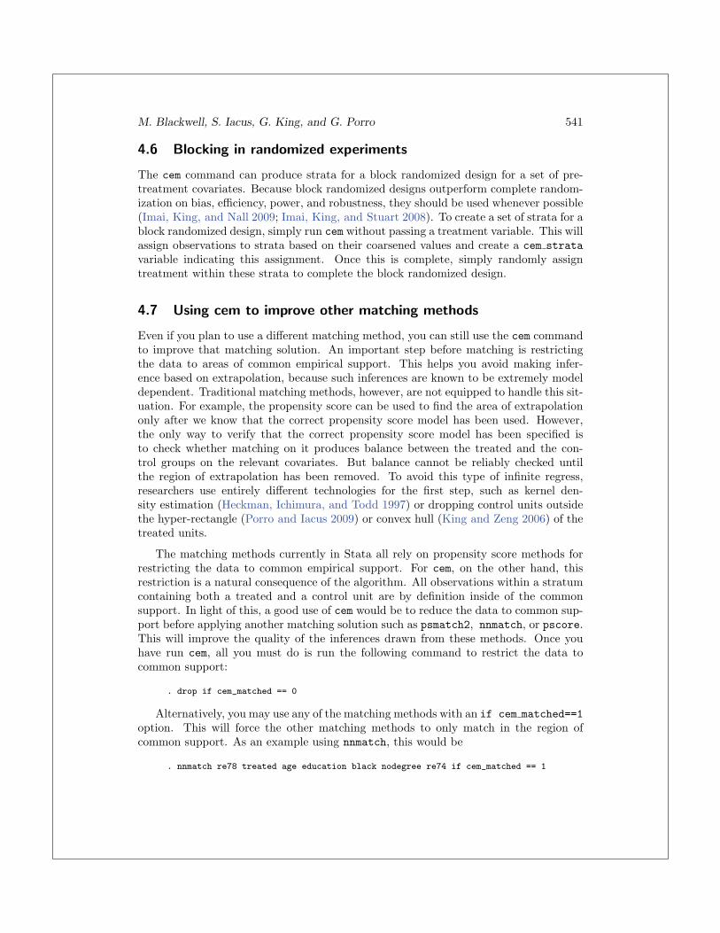
Even if you plan to use a different matching method, you can still use the cem commandto improve that matching solution. An important step before matching is restrictingthe data to areas of common empirical support. This helps you avoid making infer-ence based on extrapolation, because such inferences are known to be extremely modeldependent. Traditional matching methods, however, are not equipped to handle this sit-uation. For example, the propensity score can be used to find the area of extrapolationonly after we know that the correct propensity score model has been used. However,the only way to verify that the correct propensity score model has been specified isto check whether matching on it produces balance between the treated and the con-trol groups on the relevant covariates. But balance cannot be reliably checked untilthe region of extrapolation has been removed. To avoid this type of infinite regress,researchers use entirely different technologies for the first step, such as kernel den-sity estimation (Heckman, Ichimura, and Todd 1997) or dropping control units outsidethe hyper-rectangle (Porro and Iacus 2009) or convex hull (King and Zeng 2006) of thetreated units.
The matching methods currently in Stata all rely on propensity score methods forrestricting the data to common empirical support. For cem, on the other hand, thisrestriction is a natural consequence of the algorithm. All observations within a stratumcontaining both a treated and a control unit are by definition inside of the commonsupport. In light of this, a good use of cem would be to reduce the data to common sup-port before applying another matching solution such as psmatch2, nnmatch, or pscore.This will improve the quality of the inferences drawn from these methods. Once youhave run cem, all you must do is run the following command to restrict the data tocommon support:
. drop if cem_matched == 0
Alternatively, you may use any of the matching methods with an if cem matched==1option. This will force the other matching methods to only match in the region ofcommon support. As an example using nnmatch, this would be
. nnmatch re78 treated age education black nodegree re74 if cem_matched == 1

542 Coarsened exact matching
Of course, you may apply this idea to any matching method in Stata, not just the oneslisted here.
5 The cem command
5.1 Syntax
cem varname1[(cutpoints1)
] [varname2
[(cutpoints2)
] ]...[
, treatment(varname) showbreaks autocuts(string) k2k imbbreaks(string)
miname(string) misets(#)]
5.2 Description
cem implements the CEM method described in Iacus, King, and Porro (2008). The maininputs for cem are the variables to use (varname#) and the cutpoints that define thecoarsening (cutpoints#). The latter argument is set in parentheses after the name ofthe relevant variable. Users can either specify cutpoints for a variable or allow cem toautomatically coarsen the data based on an automatic coarsening algorithm, chosen bythe user. To specify a set of cutpoints for a variable, place a numlist in parenthesesafter the variable’s name. To specify an automatic coarsening, place a string indicatingthe binning algorithm to use in parentheses after the variable’s name. To create acertain number of equally spaced cutpoints including the extreme values, say, 10, place#10 in the parentheses (using #0 will force cem into not coarsening the variable at all).Omitting the parenthetical statement after the variable name tells cem to use the defaultbinning algorithm, itself set by autocuts().
Character variables are ignored by cem. These variables will need to be convertedinto numeric variables by using encode. Coarsening variables that are not ordinal mustbe done before running cem by using the recode command, as described above.
5.3 Options
treatment(varname) sets the treatment variable used for matching. If omitted, cemwill simply sort the observations into strata based on the coarsening and not returnany output related to matching.
showbreaks displays the cutpoints used for each variable.
autocuts(string) sets the default automatic coarsening algorithm. The default isautocuts(sturges). Any variable without a cutpoints# argument after its namewill use the autocuts() option.
k2k, by randomly dropping observations, produces a matching result that has the samenumber of treated and control units in each matched strata.

M. Blackwell, S. Iacus, G. King, and G. Porro 543
imbbreaks(string) sets the coarsening method for the imbalance checks printed af-ter cem runs. This should match whichever method is used for imbalance checkselsewhere. If either cem or imbalance has been run and there is a r(L1 breaks)available, this will be the default. Otherwise, the default is imbbreaks(scott).
miname(string) specifies the root of the filenames of the imputed dataset. They shouldbe in the working directory. For example, if you specified miname(imputed), thenthe filenames would be imputed1.dta, imputed2.dta, and so on.
misets(#) specifies the number of imputed datasets to be used for matching.
5.4 Output
The output cem returns depends on the inclusion of a treatment variable. If the treat-ment variable is provided, cem will match and return the following three variables inthe current dataset:
cem strata is the strata number assigned to each observation by cem.
cem matched is 1 for a matched observation and 0 for an unmatched observation.
cem weights is the weight of the stratum for each observation. Strata with unmatchedunits are given a weight of 0, and treated observations are given a weight of 1.
When using the multiple-imputation features, cem outputs the cem treat variable,which is the treatment vector used for matching. cem applies the same combinationrule to treatment as to strata.
If the options for multiple imputation are used, cem saves each of these variables ineach of the imputed datasets, allowing for easy use in commands like miest.
The following are stored as saved results in Stata’s memory:
Scalarsr(n strata) number of stratar(n groups) number of treatment levelsr(n mstrata) number of strata with matchesr(n matched) number of matched observationsr(L1) multivariate imbalance measure
Macrosr(varlist) covariate variables usedr(treatment) treatment variabler(cem call) call to cemr(L1 breaks) break method used for L1 distance
Matricesr(match table) table of treatment versus matchedr(groups) tabulation of treatment variabler(imbal) univariate imbalance measures
If the treatment variable is omitted (e.g., for blocking), then the only outputs arecem strata, r(n strata), r(varlist), and r(cem call).

544 Coarsened exact matching
6 The imbalance command
6.1 Syntax
imbalance varlist[if
] [in
] [, treatment(varname) breaks(string)
miname(string) misets(#) useweights]
6.2 Description
imbalance returns a number of measures of imbalance in covariates between treatmentand control groups. A multivariate L1 distance, univariate L1 distances, and differencein means and empirical quantiles difference are reported. The L1 measures are computedby coarsening the data according to breaks() and comparing across the multivariatehistogram. See Iacus, King, and Porro (2008) for more details on this measure.
6.3 Options
treatment(varname) sets the treatment variable used for the imbalance checks.
breaks(string) sets the default automatic coarsening algorithm. If cem or imbalancehas been run and there is a r(L1 breaks) available, this will be the default. Other-wise, the default is breaks(scott). It is not incredibly important which method isused here as long as it is consistent.
miname(string) specifies the root of the filenames of the imputed dataset. They shouldbe in the working directory. For example, if you specified miname(imputed), thenthe filenames would be imputed1.dta, imputed2.dta, and so on.
misets(#) sets the number of imputed datasets to be used for matching.
useweights makes imbalance use the weights from the output of cem. This is usefulfor checking balance after running cem.
6.4 Saved results
Scalarsr(L1) multivariate imbalance measure
Macrosr(L1 breaks) break method used for L1 distance
Matricesr(imbal) univariate imbalance measures

M. Blackwell, S. Iacus, G. King, and G. Porro 545
7 ReferencesAbadie, A., A. Diamond, and J. Hainmueller. Forthcoming-a. Synthetic control methods
for comparative case studies: Estimating the effect of California’s tobacco controlprogram. Journal of the American Statistical Association.
———. Forthcoming-b. Synth: An R package for synthetic control methods in com-parative case studies studies: Estimating the effect of California’s tobacco controlprogram. Journal of Statistical Software.
Abadie, A., D. Drukker, J. Leber Herr, and G. W. Imbens. 2004. Implementing matchingestimators for average treatment effects in Stata. Stata Journal 4: 290–311.
Becker, S. O., and A. Ichino. 2002. Estimation of average treatment effects based onpropensity scores. Stata Journal 2: 358–377.
Crump, R. K., V. J. Hotz, G. W. Imbens, and O. A. Mitnik. 2009. Dealing with limitedoverlap in estimation of average treatment effects. Biometrika 96: 187–199.
Heckman, J. J., H. Ichimura, and P. Todd. 1997. Matching as an econometric evaluationestimator: Evidence from evaluating a job training program. Review of EconomicStudies 64: 605–654.
Ho, D. E., K. Imai, G. King, and E. A. Stuart. 2007. Matching as nonparametricpreprocessing for reducing model dependence in parametric causal inference. PoliticalAnalysis 15: 199–236.
Honaker, J., G. King, and M. Blackwell. 2006. Amelia II: A program for missing data.http://gking.harvard.edu/amelia/docs/amelia.pdf.
Iacus, S. M., G. King, and G. Porro. 2008. Matching for causal inference without balancechecking. http://gking.harvard.edu/files/cem.pdf.
Imai, K., G. King, and C. Nall. 2009. The essential role of pair matching in cluster-randomized experiments, with application to the Mexican Universal Health InsuranceEvaluation. Statistical Science 24: 29–53.
Imai, K., G. King, and E. A. Stuart. 2008. Misunderstandings between experimentalistsand observationalists about causal inference. Journal of the Royal Statistical Society,Series A 171: 481–502.
King, G., J. Honaker, A. Joseph, and K. Scheve. 2001. Analyzing incomplete politicalscience data: An alternative algorithm for multiple imputation. American PoliticalScience Review 95: 49–69.
King, G., and L. Zeng. 2006. The dangers of extreme counterfactuals. Political Analysis14: 131–159.
LaLonde, R. J. 1986. Evaluating the econometric evaluations of training programs.American Economic Review 76: 604–620.

546 Coarsened exact matching
Leuven, E., and B. Sianesi. 2003. PSMATCH2: Stata module to perform full Mahalanobisand propensity score matching, common support graphing, and covariate imbalancetesting. Statistical Software Components S432001, Department of Economics, BostonCollege. http://ideas.repec.org/c/boc/bocode/s432001.html.
Porro, G., and S. M. Iacus. 2009. Random recursive partitioning: A matching methodfor the estimation of the average treatment effect. Journal of Applied Econometrics24: 163–185.
StataCorp. 2009. Stata 11 Multiple-Imputation Reference Manual. College Station, TX:Stata Press.
About the authors
Matthew Blackwell is a doctoral candidate in the Department of Government at HarvardUniversity and is an affiliate of the Institute for Quantitative Social Science.
Stefano M. Iacus is an associate professor in the Department of Economics, Business, andStatistics at the Universita degli Studi di Milano, Italy.
Gary King is the Albert J. Weatherhead III University Professor and Director of the Institutefor Quantitative Social Science at Harvard University.
Giuseppe Porro is an associate professor of Economic Policy in the Department of Economicsand Statistics at the Universita degli Studi di Trieste, Italy.