catastrophe pricing - international actuarial association sorts of issues that affect catastrophe...

Catastrophe Pricing

Prepared by John De Ravin

Presented to IACA Program part of the IACA, PBSS & IAAust Colloquium

31 October – 5 November 2004

This paper has been prepared for the IACA, PBSS & IAAust Colloquium 2004. The IACA, PBSS & IAAust wishes it to be understood that opinions put forward herein are not necessarily those of IACA, PBSS & IAAust and are not

responsible for those opinions.

© 2004 International Association of Consulting Actuaries

The Institute of Actuaries of Australia Level 7 Challis House 4 Martin Place

Sydney NSW Australia 2000 Telephone: +61 2 9233 3466 Facsimile: +61 2 9233 3446

Email: [email protected] Website: www.actuaries.asn.au

mailto:[email protected]

http://www.actuaries.asn.au/

Catastrophe Pricing

Catastrophe Pricing 1 Introduction..........................................................................................................3 2 Why are Catastrophe Premiums so Volatile? ...................................................4

2.1 ECONOMICS OF THE REINSURANCE INDUSTRY ................................................4 2.2 TECHNICAL PRICING – THE RISK PREMIUM.....................................................5

3 Profit Loadings.....................................................................................................7 3.1 RETURN ON EQUITY BY LINE OF BUSINESS .....................................................7 3.2 LOADING ON FLUCTUATIONS ..........................................................................8 3.3 APPLICATION TO CATASTROPHE PREMIUM RATING .........................................9

4 Pricing to Reflect Aggregate Exposures ..........................................................11 4.1 EXPOSURE BUDGETS.....................................................................................11 4.2 SIMPLIFIED EXAMPLE ...................................................................................12

5 Implications of Retaining a Major Catastrophe Risk ....................................14 5.1 THE RETENTION OPTION................................................................................14 5.2 TERMINOLOGY AND ASSUMPTIONS...............................................................14 5.3 CAPITAL REQUIRED ......................................................................................15 5.4 DATA ............................................................................................................16 5.5 METHODOLOGY ............................................................................................16 5.6 HYPOTHETICAL INSURER GROUP ..................................................................16 5.7 CAPITAL REQUIRED TO SUPPORT THE BUSINESS...........................................17 5.8 COSTS OF THE EARTHQUAKE RISK.................................................................18 5.9 COMMENTS ON RESULTS ...............................................................................20

6 Conclusion ..........................................................................................................21 References...................................................................................................................22

IACA/PBSS/IAAust Colloquium, Sydney 2004

Catastrophe Pricing

1 Introduction In the present hardening reinsurance market, it is natural for insurers, finding that their reinsurance expense has increased, to ask themselves a number of questions about their reinsurance programmes. Amongst there questions are:

1. Why are catastrophe premiums so volatile?

2. What loadings do reinsurers incorporate into their catastrophe rates, and why?

3. How do reinsurers vary their prices according to their existing exposures by geographical zone?

4. What would be the pricing consequences of retaining a significant catastrophe exposure in an otherwise balanced portfolio?

This paper is an attempt to provide an answer to these questions. The views expressed are however the opinions of the author and do not necessarily reflect the views of his employer.


Catastrophe Pricing

2 Why are Catastrophe Premiums so Volatile? In this section we note that the catastrophe premium rates charged in the Australian market are relatively volatile and we consider two explanations as to why this should be the case: one based on the macroeconomic facts of the reinsurance industry, and the other a more statistical explanation regarding uncertainty in the technical pricing.

2.1 Economics of the Reinsurance Industry

The author recollects reading an explanation of the factors underlying price volatility in an elementary actuarial textbook on investments that was written some forty years ago. The observation was made that if an industry is capital intensive, and if the marginal costs of providing the industry’s product are very low, then the price of the product will be volatile during economic cycles. The example that was given was shipping freight. When the demand for shipping services outstrips supply, then importers and exporters will be prepared to pay high prices in order to get their shipments delivered. However, when supply outstrips demand, the low marginal cost of shipping relative to the capital component of having a huge investment in idle ships means that shipowners will compete for business and will drive freight rates down to extremely low levels. Of these two factors, reinsurance is capital intensive, though the marginal costs of reinsurance are higher than those of the shipping industry. It is expensive and costly to have idle capital sitting by without earning a return, and shareholders will soon tire of that situation. Similarly for capital subscribed to the insurance industry. Shareholders will not accept subnormal returns relative to those that should be earned commensurate with the risk of writing insurance business. Insurance stocks are riskier than the market, due to their greater volatility, which is reflected in "beta” values in excess of unity. Typical insurance “betas” are of the order of 1.2 to 1.3. This means that insurance shares need to earn a rate of return in excess of the market rate of return in order to satisfy their shareholders that their capital is being put to good use. There are a number of reasons why capital globally withdrew from the industry over the last few years. These include:

• Major losses such as the September 11, 2001 World Trade Centre loss, the largest insurance loss known to mankind

• Emergence of asbestos claims as a major source of unreserved losses

• Significant falls in the asset markets that occurred over calendar year 2002

The volatility in reinsurance catastrophe rates does not need to be seen as reinsurers “rebuilding” their balance sheets, though there is little doubt that they would do this if they could. There is a stronger rationale for assuming that the emerging prices are a simple function of supply and demand. Hardening rates will of course make it attractive for new capital to enter the market, and in fact there have been a number of opportunistic start-ups, particularly in Bermuda.


Catastrophe Pricing

2.2 Technical Pricing – the Risk Premium

However, the above is not a complete explanation of the volatility of catastrophe rates. We noted above that there is a significant marginal cost to underwriting reinsurance business, much more so than in ship freight. That marginal cost (i.e. the cost of claims and the direct costs of handling policies and claims) has not however provided the sort of minimum pricing base that one would normally have expected of a rational industry. The reason for that, I believe, is the following. Catastrophe events are of their nature infrequent events. The events that would cause significant catastrophe claims are rare events. The sorts of issues that affect catastrophe pricing are what would be the total losses in respect of a “one in one hundred year” Sydney earthquake loss event, or a “one in two hundred year” Brisbane windstorm, or a “one in fifty year” NSW bushfire. The very rarity of the events combined with the problem of finding good estimates for historical “as-if” losses means that it is not possible to obtain very reliable estimates of severity of losses or the probability with which extreme events occur. One can of course attempt to model natural catastrophe events and indeed, there are a number of commercially available packages as well as proprietary models that do indeed attempt to model the impact of catastrophes on a particular insurer’s portfolio. In the USA, four major providers of catastrophe models are Risk Management Solutions (RMS), EQECAT (a joint venture between an engineering firm and Guy Carpenter), Applied Insurance Research (AIR) and Tillinghast, a firm of consulting actuaries. These providers cater to different catastrophe type events and produce different answers for the cost of any specified event. However, the rarer the event being modelled, the less likely it is that the modelled phenomenon will behave in the manner predicted. Modelling involves fitting statistical distributions to the past history of losses, but where data are necessarily scarce, the reliability of model results is most open to question. Both the form of the model and the technique of parameterising the model to obtain the best fit to observed experience may vary from one model builder to another. Indeed the various catastrophe models that have been developed to model a range of natural catastrophes do produce markedly differing results in terms of the annualised cost of claims from the modelled catastrophes, at least for some perils in some regions, as indeed would be expected unless there was some form of calibration of results of one model against another. So the situation is that there may be a wide range of varying estimates of the cost of natural catastrophe and no-one really knows the true long-term cost of any particular class of catastrophes; we can only make a variety of estimates and the widely varying estimates of the costs of some perils from different models should indicate to us the uncertainty inherent in any of the estimation models. In short, the reinsurance industry is by its capital intensive nature prone to cyclicality and moreover, the lack of any reliable and agreement as to the most basic costing of the cover means that the market clearing cost of reinsurance is determined by supply and demand considerations more than the technical rate; this occurs precisely because


Catastrophe Pricing

the technical rate is to some extent unclear. Instead of there being “the” technical rate there is a range of technical rates, varying according to who has prepared the model on which the risk premiums are to be based. When the supply of reinsurance capital is depleted relative to the demand for catastrophe reinsurance support, then buyers are likely to pay a price that lies at the high end of the range of calculated technical rates. Conversely, when the supply of capital is extensive relative to demand, it is likely that insurers will be able to place business with reinsurers willing to quote at the low end of the range of technical rates. If the range of technical rates is wide, then this cyclical process may lead to significant variations in the ruling market rates over time.


Catastrophe Pricing

3 Profit Loadings In the past few years there has been an increased focus on profit in both the Australian general insurance market and internationally. There has been a depletion in the volume of capital in both the local direct insurance market and international reinsurance markets highlighted locally by the failure of a large underwriter and internationally by a diminution of the capital resulting in downgrades to the claims paying rating of many reinsurance groups. In this Section of the paper, a possible method of loading the risk premium for profit is considered and its implications for catastrophe premium rates are illustrated.

3.1 Return on Equity by Line of Business

Commonly insurers are trying to achieve a return on equity (ROE) at some specified rate, although it is possible that insurers use other targets such as added value targets after the cost of capital (or target rate of return on capital) has been achieved. Because the “Return” in the ROE definition is considered in relation to a denominator of “Equity”, it is important to consider exactly what comprises the “Equity” and how it is to be allocated amongst the different classes of business. It is true that the regulator has defined the capital requirements associated with particular lines of business in terms of the ratio of capital to premiums and the ratio of capital to the outstanding claims provision. However, in principle, each company should perform their own allocation of capital to the various lines of business. Really there are two questions: 1 How much capital do we consider is necessary to operate our business at the

desired level of security?

2 How is this capital to be allocated between lines of business?

These questions are not trivial. The board of the insurer can be expected to have a view on the general level of capital that is required and this must be taken into account as the question of how much capital is needed is partially a matter of choice of the degree of security that the insurer wishes to provide to its clients that it will pay its obligations, and there is a trade-off between security and growth (the more secure the business the less scope there is for rapid growth of the portfolio). Even when the first decision (how much capital?) has been taken the second question is not mathematically trivial. Suppose that an insurer has decided, on the basis of statistical analyses of its portfolio and the board’s preferences in terms of the security to be offered to policyholders, that the total capital required to support its given portfolio is (say) $60 million. The insurer may write premiums that we will assume total $100 million. Does this mean that the company will allocate 60 cents of capital to every dollar of premiums that it writes? The answer to this question is that there are many reasons why capital should not be allocated pro rata to premiums.

1. The uncertainty of the business is partly generated by the outstanding claims liabilities as well as the premium liabilities.


Catastrophe Pricing

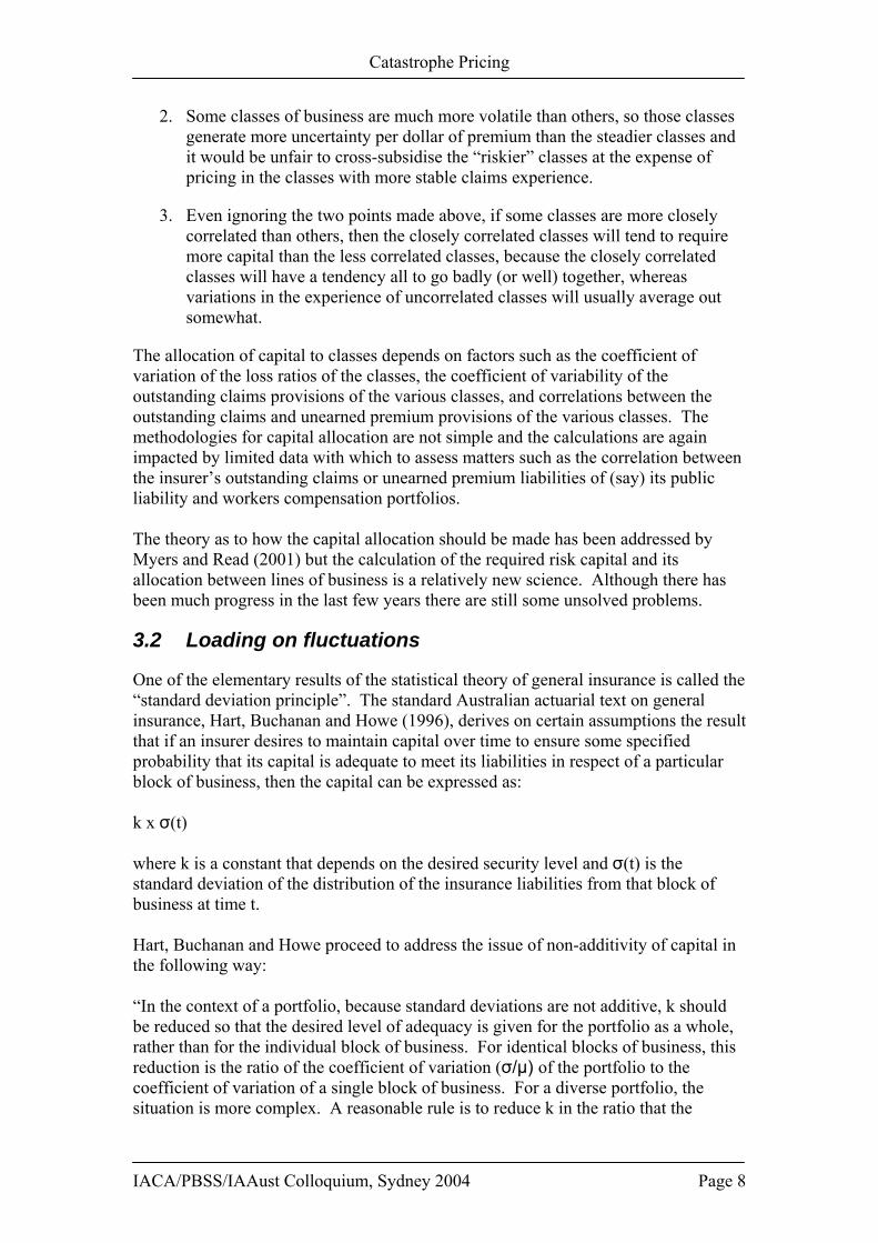
2. Some classes of business are much more volatile than others, so those classes generate more uncertainty per dollar of premium than the steadier classes and it would be unfair to cross-subsidise the “riskier” classes at the expense of pricing in the classes with more stable claims experience.

3. Even ignoring the two points made above, if some classes are more closely correlated than others, then the closely correlated classes will tend to require more capital than the less correlated classes, because the closely correlated classes will have a tendency all to go badly (or well) together, whereas variations in the experience of uncorrelated classes will usually average out somewhat.

The allocation of capital to classes depends on factors such as the coefficient of variation of the loss ratios of the classes, the coefficient of variability of the outstanding claims provisions of the various classes, and correlations between the outstanding claims and unearned premium provisions of the various classes. The methodologies for capital allocation are not simple and the calculations are again impacted by limited data with which to assess matters such as the correlation between the insurer’s outstanding claims or unearned premium liabilities of (say) its public liability and workers compensation portfolios. The theory as to how the capital allocation should be made has been addressed by Myers and Read (2001) but the calculation of the required risk capital and its allocation between lines of business is a relatively new science. Although there has been much progress in the last few years there are still some unsolved problems.

3.2 Loading on fluctuations

One of the elementary results of the statistical theory of general insurance is called the “standard deviation principle”. The standard Australian actuarial text on general insurance, Hart, Buchanan and Howe (1996), derives on certain assumptions the result that if an insurer desires to maintain capital over time to ensure some specified probability that its capital is adequate to meet its liabilities in respect of a particular block of business, then the capital can be expressed as: k x σ(t) where k is a constant that depends on the desired security level and σ(t) is the standard deviation of the distribution of the insurance liabilities from that block of business at time t. Hart, Buchanan and Howe proceed to address the issue of non-additivity of capital in the following way: “In the context of a portfolio, because standard deviations are not additive, k should be reduced so that the desired level of adequacy is given for the portfolio as a whole, rather than for the individual block of business. For identical blocks of business, this reduction is the ratio of the coefficient of variation (σ/µ) of the portfolio to the coefficient of variation of a single block of business. For a diverse portfolio, the situation is more complex. A reasonable rule is to reduce k in the ratio that the


Catastrophe Pricing

coefficient of variation of a block of business equal in size to the whole portfolio would bear to the coefficient of variation of the actual block of business at its date of issue. The extent of such a reduction depends on the relative sizes of the portfolio and of the block of business and on the relative importance of independent and systemic variation.” In this somewhat complex situation, Hart, Buchanan and Howe discuss a range of possible “pricing principles” or methods by which the insurer determines how the total loading to be collected from all insureds is to be allocated to individual contracts. Various options are available to insurers, and one that has some theoretical support is the “standard deviation principle” of pricing, according to which the insurer charges a profit loading in proportion to the standard deviation of the modelled loss distribution of individual contracts. The “standard deviation principle” is indeed sometimes adopted in practice as a method of determining loadings for catastrophe reinsurance.

3.3 Application to catastrophe premium rating

That result allows us to examine the way in which profit loadings must be applied to catastrophe layers. For the sake of a simple illustration, suppose that a catastrophe insurer decides that it wishes to maintain capital in respect of identical blocks of catastrophe business equal to a multiple of one half of one standard deviation of its liabilities. Suppose a notional catastrophe programme comprised 99 small excess layers, each of $1 million, in excess of the direct insurer’s $1million retention. (Of course, this is an unrealistic example of a programme, as in practice the retention will be more than $1million and there will not be so many small layers; this example is merely intended to be illustrative). Then the layers of the programme are: Layer 1: $1million in excess of $1 million Layer 2: $1 million in excess of $2 million Layer 3: $1 million in excess of $3 million …… Layer 99: $1 million in excess of $99 million. Now to each of these layers we can attribute a probability of the layer being burned by a catastrophe, say pi for layer i of the 99 layers. Then assuming that all losses to the programme occur in even multiples of $1 million (effectively ignoring partial losses to a layer) the risk premium for layer i, which will have been derived from the insurer’s and reinsurer’s catastrophe risk modelling processes, is simply 1,000,000 pi Note that the pi values may vary significantly from layer to layer; in particular, the lower layers are probably quite likely to be “hit” by a catastrophe but the higher layers will be much less likely to be affected, having probability say 0.01 (i.e. the insurer would be covered for a one in one hundred year event). For the sake of our illustration let us assume that p1 has a value of 0.8 but that p10 is 0.1, and p99 is 0.01.


Catastrophe Pricing

So the risk premium for the first layer is $800,000 but the risk premium for the 10th and 99th layers are $100,000 and $10,000 respectively. Assuming total loss to any affected layer, then the formula for the standard deviation has a very simple form: it is 1,000,000√(pi(1- pi)). Equivalently, if the rate on line ROLi of layer i is expressed as a percentage, this formula becomes: 10,000√(ROLi(100- ROLi)). Finally, assuming that the insurer requires a return of 10% of capital required in respect of these contracts, we can compute the required profit loadings. We can summarise the results in the following table: Table 1: Profit margins for different catastrophe layers Layer Probability layer

affected Risk

Premium Required

capital Required

profit Profit

margin 1 0.8 $800,000 $200,000 $20,000 4.0% 10 0.1 $100,000 $150,000 $15,000 15.0% 99 0.01 $10,000 $49,750 $4,975 49.8%

The main point to note about the above table is that it demonstrates that the profit margin required is a function that varies importantly with the probability of occurrence of the event. Larger amounts of capital are required per dollar of written premiums to support unlikely events with high sums insured relative to stabler classes with higher claim frequency but smaller sums insured, resulting in lower overall volatility.


Catastrophe Pricing

4 Pricing to Reflect Aggregate Exposures 4.1 Exposure Budgets

Catastrophe reinsurers accept the large though unlikely risks in return for a small part of the original premium. Whilst this means that the reinsurer is contributing to the direct insurer’s objectives of limiting their risk and ensuring that their portfolios meet statutory requirements, nevertheless, reinsurers must also manage their accumulation risks in the same way as their customers. Reinsurers will establish budgets in terms of the maximum exposures that they can accept in any particular geographical zone. In Australia, catastrophe exposures are generally analysed by ICA zone and there are 42 such zones into which exposures are categorised. In general, the choice of zones is intended to be such that a catastrophic loss would not normally impact on more than one ICA zone, but that assumption does not hold strictly true; particularly in recent experience, bushfires have tended to rage over more than one zone causing losses simultaneously in several zones. The large international reinsurers approach the task of capital management and risk management from a global perspective and so at a Head Office level; they prepare budgets of capital to be allocated to the various operating divisions by geographical zone, along with maximum exposures on a PML basis. Accordingly, the local reinsurance underwriters must limit their acceptance of risk in accordance with this budget. From a mathematical perspective, this means that there is an additional constraint on the reinsurance underwriter. Not only must they win business, and at a price that will provide a return for their shareholders, but also, they are unable to accept more business in certain geographical zones than they have been allocated. For a reinsurer with abundant capital available for the market in which an underwriter is operating, there may not be any problem with accepting whatever business the underwriter can write on terms considered acceptable. However, if capital is in shorter supply, the underwriter may face a real constraint in terms of acceptance of business. At an extreme, the underwriter may not be able to accept any further business with exposure to the particular ICA zone or zones where the reinsurer’s budget is already fully utilised. Even assuming that the budget for a particular zone is not yet fully utilised, so long as the accumulation is approaching the budgeted level, then the underwriter needs to take that fact into account when pricing any particular catastrophe portfolio that is offered. Clearly, the underwriter should tend to avoid accepting further portfolios that are relatively heavily exposed to the ICA zones where the underwriter is already more fully committed. From an actuarial perspective, one way in which the reinsurance catastrophe underwriter can do that is to vary the prices charged by ICA zone to make its quotations less attractive if the subject portfolio is relatively heavily weighted and conversely more attractive if the portfolio being quoted on is less heavily weighted in those other areas. Of course, in practice, the reinsurance underwriter also needs to consider the potential impact of significant unanticipated variations in the capacity or terms offered by the reinsurer on the insurer/reinsurer relationship.


Catastrophe Pricing

4.2 Simplified Example

To illustrate the concept of the previous section we will use a simple and totally hypothetical example following Reinhart and Mango (2001). Suppose that in the USA there are only four major cat events that could impact on reinsurers: San Francisco earthquake, Los Angeles earthquake, Florida Hurricane, and New Mexico earthquake. Suppose that the probability of each event is 1% and that the average losses, given that an event occurs, are as set out in the table below. Finally, suppose that the reinsurer requires a profit loading of 30% on the portfolio to support the capital required. Table 2: Risk premiums and profit loadings for various perils Event/Peril Probability Average Insured

Losses Risk

Premium Profit

Loading San Francisco Earthquake

1% $4 billion $40M $12M

Los Angeles Earthquake

1% $3 billion $30M $9M

Florida Hurricane


New Mexico Earthquake


Total 4% $10 billion $100M $30M If a reinsurer is already particularly heavily exposed to losses in San Francisco relative to losses in Florida and New Mexico then it is possible to design a pricing basis under which the reinsurer may be able to achieve the same average profit loading but at the same time include a relative bias towards accepting portfolios with relatively less San Francisco risk and relatively higher exposure to Florida and New Mexico. This involves developing a set of weights to apply to the profit loading so that the total profit that will be derived is intended to be the same though the quotations to insurers with portfolios in the area to which the reinsurers are already heavily exposed will be penalised and the benefits derived from that will be applied to quotations from those areas where the reinsurer has relatively less exposure. For example, in the simple example above, the factors 1.33, 1, 0.67 and 0.33 may be applied to the profit margin from exposures in San Francisco, Los Angeles, Florida and New Mexico respectively and the total profit loadings collected will be the same assuming that the reinsurer writes the same cross section of business, as shown in the following table.


Catastrophe Pricing

Table 3: Adjusted profit margins for various perils Event/Peril Risk

Premium Flat 30% profit loading

Multiplier New Profit Loading

New Profit

Margin%San Francisco Earthquake

$40M $12M 1.33 $16M 40%

Los Angeles Earthquake

$30M $9M 1.00 $9M 30%

Florida Hurricane

$20M $6M 0.67 $4M 20%

New Mexico Earthquake

$10M $3M 0.33 $1M 10%

Total $100M $30M $30M In reality what will be achieved is a re-balancing of the portfolio away from clients with heavy exposure towards San Francisco and towards clients with a heavy exposure in Florida and New Mexico.


Catastrophe Pricing

5 Implications of Retaining a Major Catastrophe Risk 5.1 The retention option

Of course, from the insurer’s point of view it is not compulsory to reinsure a catastrophe risk, although in these days of tighter risk management the net exposures of the insurer to catastrophe events will be examined closely by not only the reinsurance manager, but also senior management, the board and by the regulator. In this section of the paper, we examine a simple pricing model in the somewhat simplified context of an insurer with a portfolio that we will categorise simplistically as being comprised of two components:

1 A component that is not exposed to a catastrophe risk; and 2 A component that is exposed to a single large catastrophe risk.

In fact, the New Zealand insurance market can be considered to be some sort of approximation to this simplistic model. New Zealand general insurers underwrite portfolios of property and casualty business in the usual way, but New Zealand is in a seismically active zone and property risks in the Wellington area are subject to an earthquake risk with relatively low return periods. The government has established the Earthquake Commission (EQC), which offers insurance to members of the public for sums insured of up to $100,000 on buildings and up to $20,000 on contents. Insurers are exposed to the earthquake risk however via their commercial property portfolios (not covered by the EQC) and also, to the extent that they offer cover to individual householders in excess of the benefits provided by the EQC, to an accumulation loss in the event of a catastrophe. The focus of this section of the paper is the profit margin that should be included in the pricing of the special catastrophe risk, an event with low frequency but high cost when it does occur, to maintain the insurer’s required return on equity. A very simple spreadsheet has also been prepared which illustrates some of the conclusions of this paper in the context of the Wellington earthquake risk.

5.2 Terminology and Assumptions

We need to introduce some terminology and assumptions. Define: P = Premiums (net of any expense loadings) underwritten by the insurer excluding

the earthquake risk σ2 = Variance of claims occurring in a particular year according to the modelled

loss distribution C = Cost of claims occurring in a year (other than from the earthquake risk)


Catastrophe Pricing

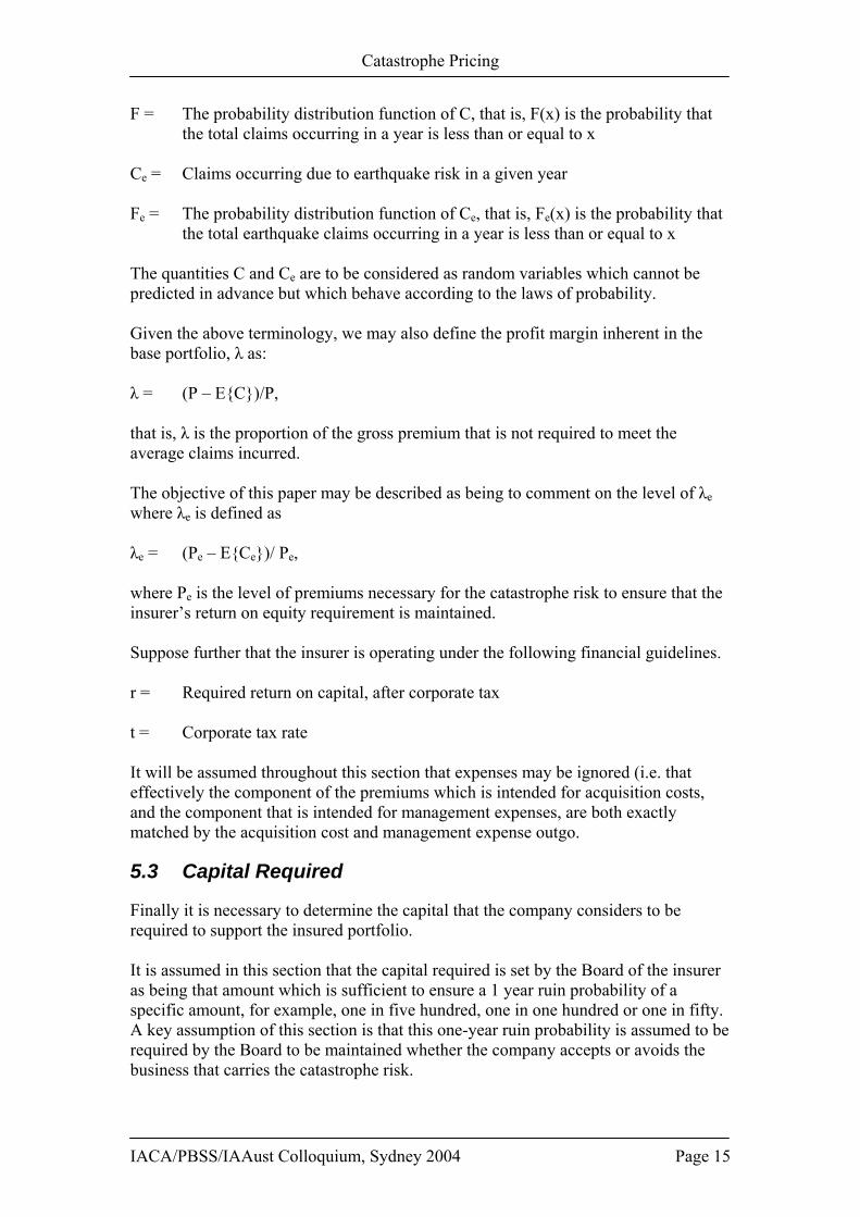
F = The probability distribution function of C, that is, F(x) is the probability that the total claims occurring in a year is less than or equal to x

Ce = Claims occurring due to earthquake risk in a given year Fe = The probability distribution function of Ce, that is, Fe(x) is the probability that

the total earthquake claims occurring in a year is less than or equal to x The quantities C and Ce are to be considered as random variables which cannot be predicted in advance but which behave according to the laws of probability. Given the above terminology, we may also define the profit margin inherent in the base portfolio, λ as: λ = (P – E{C})/P, that is, λ is the proportion of the gross premium that is not required to meet the average claims incurred. The objective of this paper may be described as being to comment on the level of λe where λe is defined as λe = (Pe – E{Ce})/ Pe, where Pe is the level of premiums necessary for the catastrophe risk to ensure that the insurer’s return on equity requirement is maintained. Suppose further that the insurer is operating under the following financial guidelines. r = Required return on capital, after corporate tax t = Corporate tax rate It will be assumed throughout this section that expenses may be ignored (i.e. that effectively the component of the premiums which is intended for acquisition costs, and the component that is intended for management expenses, are both exactly matched by the acquisition cost and management expense outgo.

5.3 Capital Required

Finally it is necessary to determine the capital that the company considers to be required to support the insured portfolio. It is assumed in this section that the capital required is set by the Board of the insurer as being that amount which is sufficient to ensure a 1 year ruin probability of a specific amount, for example, one in five hundred, one in one hundred or one in fifty. A key assumption of this section is that this one-year ruin probability is assumed to be required by the Board to be maintained whether the company accepts or avoids the business that carries the catastrophe risk.


Catastrophe Pricing

5.4 Data

Data on the distribution of the earthquake risk were obtained from the QUAKE model, a proprietary model of the Munich Reinsurance Company. The input data were based on the observed past seismic activity in each of the New Zealand “Cresta zones” and the likely impact on a sample of Wellington commercial property risks. Two separate distributions were derived, one for specifically a Wellington portfolio and the other for a New Zealand-wide commercial property portfolio.

5.5 Methodology

The method that has been used in this section is as follows.

1. A group of hypothetical insurers is established with different portfolio volatility (before earthquake risk) the distribution of the claims incurred in a year is obtained on the assumption that the claims are distributed lognormally.

2. The capital required to support the business for each hypothetical insurer is determined on the basis of a range of specified one-year ruin probabilities.

3. The distribution of the total claims if the insurer takes on additional earthquake risk is calculated.

4. From the distribution of the total claims, the additional capital requirement is obtained to maintain the same one-year ruin probability as before.

5. The premiums necessary to provide the required rate of return on capital are calculated and the implied profit margins are calculated and presented in tabular form.

5.6 Hypothetical Insurer Group

The portfolio volatility of an insurer will depend on factors such as:

• The size of the insurer • The mix of business • The geographical distribution of business

We may consider three insurers, with varying portfolio volatilities as measured by the coefficient of variation of the retained claims distribution. Consider four insurers as set out in the following table:


Catastrophe Pricing

Table 4: Coefficients of variation for sample insurers Insurer Portfolio Volatility Coefficient of Variation (y) A Low 10% B Medium 15% C High 20% D Very High 30% Suppose that each of the four insurers has expected claims E{C} of $100 million.

5.7 Capital Required to Support the Business

We assume that the claims incurred in a year are lognormally distributed with mean E{C}=$100 million and coefficients of variation as described above. Then the capital requirement for each of the above insurers may be determined from the relationship Pr{C-P>U} = ε where U is the initial free reserves over and above the minimum solvency requirement and ε is the low one-year ruin probability set by the Board. For the assumed lognormal distribution it can be shown that the logarithm of the claims incurred is distributed as the normal distribution with mean µ and variance σ2

where: µ = ln(E{C})- σ2 /2 and σ2 = ln(1+y2) where y is the coefficient of variation. The required capital defined in terms of the one-year ruin probabilities for each of companies A, B, C and D in the above table is then set out in the following table. Table 5: Capital Requirements – No Catastrophe Risk

-------------------------One year ruin probability---------------------------------------------------------------------0.00001 0.0002 0.0005 0.001 0.002 0.005 0.01 0.02 0.05

A 52.3 41.6 38.2 35.4 32.6 28.7 25.5 22.1 17.2B 86.9 67.7 61.6 56.8 51.9 45.2 39.9 34.3 26.4C 128.2 97.7 88.1 80.8 73.4 63.3 55.4 47.3 35.8D 235.0 170.8 151.6 137.3 123.0 104.0 89.6 75.0 55.2

Thus, for example, if the Board of Insurer A sets a requirement for its capital strength that the company should not become insolvent for reasons of the random fluctuation of the claims experience more than (say) once every one thousand years, then the capital required would be $35.4 million. However, insurer D with its more volatile portfolio would need capital of $75.0 million even if its Board were prepared to


Catastrophe Pricing

tolerate a 2% probability of ruin (i.e. a one in fifty chance of becoming insolvent due to the claims experience).

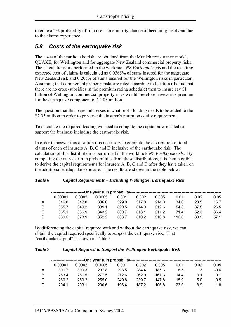
5.8 Costs of the earthquake risk

The costs of the earthquake risk are obtained from the Munich reinsurance model, QUAKE, for Wellington and for aggregate New Zealand commercial property risks. The calculations are performed in the workbook NZ Earthquake.xls and the resulting expected cost of claims is calculated as 0.0365% of sums insured for the aggregate New Zealand risk and 0.205% of sums insured for the Wellington risks in particular. Assuming that commercial property risks are rated according to location (that is, that there are no cross-subsidies in the premium rating schedule) then to insure say $1 billion of Wellington commercial property risks would therefore have a risk premium for the earthquake component of $2.05 million. The question that this paper addresses is what profit loading needs to be added to the $2.05 million in order to preserve the insurer’s return on equity requirement. To calculate the required loading we need to compute the capital now needed to support the business including the earthquake risk. In order to answer this question it is necessary to compute the distribution of total claims of each of insurers A, B, C and D inclusive of the earthquake risk. The calculation of this distribution is performed in the workbook NZ Earthquake.xls. By computing the one-year ruin probabilities from these distributions, it is then possible to derive the capital requirements for insurers A, B, C and D after they have taken on the additional earthquake exposure. The results are shown in the table below. Table 6 Capital Requirements – Including Wellington Earthquake Risk


A 346.0 342.0 336.0 329.0 317.0 214.0 34.0 23.5 16.7B 355.7 349.2 339.1 329.5 314.9 212.6 54.3 37.5 26.5C 365.1 356.9 343.2 330.7 313.1 211.2 71.4 52.3 36.4D 389.5 373.9 352.2 333.7 310.2 210.8 112.6 83.9 57.1

By differencing the capital required with and without the earthquake risk, we can obtain the capital required specifically to support the earthquake risk. That “earthquake capital” is shown in Table 3. Table 7 Capital Required to Support the Wellington Earthquake Risk


A 301.7 300.3 297.8 293.5 284.4 185.3 8.5 1.3 -0.6B 283.4 281.5 277.5 272.6 262.9 167.3 14.4 3.1 0.1C 260.2 259.2 255.0 249.8 239.7 147.8 15.9 5.0 0.5D 204.1 203.1 200.6 196.4 187.2 106.8 23.0 8.9 1.8


Catastrophe Pricing

We can make the following observations on the calculations of required capital above.

irstly, it is clear that a conservative insurer (one with a one-year ruin probability of

200

d n

ven an insurer that is prepared to take a mild risk must provide additional capital for

urn

oting that r was defined above as the required rate of return on capital, let us also

= pre-tax return on company reserves R

hen

λ = R(r-i(1-t))

other words, the profit margin in the premiums must make up the difference uired

r re-expressing this,

= R/P(r-i(1-t))

or insurers A, B, C and D, on the assumptions of a 1% one-year ruin probability, the

= 0.065

hen the values of λe are in the range 22.6% to 63.2%. Put another way, there needs

Fsay one in 200 or less) would not be likely to accept earthquake risk at all. Take Insurer B for example. If the Board of this insurer determines that it must keep capital to prevent the one-year ruin probability from falling below 0.005 (one in chance) then the capital requirement is $45.2 million to support its $100 million portfolio without earthquake exposure, but it needs capital of $212.6 million to support the portfolio if the $1 billion of Wellington commercial cover is include(with an expected cost of claims of $2 million). Additional capital of $167.3 milliois needed to support the very modest additional premiums. It is clear that Insurer B would not accept such an additional exposure under these circumstances. Ethe earthquake risk. For the 1% one-year ruin probability then the additional capital of somewhere between $8.3 million and $23.0 million which is required must be serviced and the difference between the insurer’s cost of capital and the rate of retearned on the technical reserves must be provided by pricing margins for the earthquake risk. Ndefine: i T P Inbetween the risk-free earnings rate on invested reserves and the rate of return reqby the shareholders in return for providing the capital to support the insurance risk. O λ Fratio R/P ranges from 4.0 to 11.2. If: i R = 0.125 T = 0.33 Tto be a loading of between 1/(1-0.226) and 1/(1-0.632) or from 29% to 170%.


Catastrophe Pricing

5.9 Comments on results

The loadings to be applied in the pricing of catastrophe risk depends on a range of factors including:

• The volatility of the base portfolio • The capital policy of the insurer, which is partly a function of the insurer’s

attitude to the chance of insolvency In one investigation of four hypothetical insurers it was necessary to load the cost of the earthquake cover by loadings from 29% to 170%.


Catastrophe Pricing

6 Conclusion In the introduction of this paper, four questions were posed. This section concludes the paper with a brief précis of my suggested answers. Question Suggested Answer 1 Why are catastrophe premiums so

volatile? Catastrophe premiums are volatile because the capital-intensive nature of the industry encourages an insurance cycle particularly when combined with significant uncertainty as to the true underlying cost of catastrophes due to the lack of sufficient credible statistical evidence.

2 What loadings do reinsurers incorporate into their catastrophe rates, and why?

Apart from the obvious loadings for expenses and brokerage, reinsurers must charge a gross premium that provides their shareholders with a required rate of return on capital. Typically profit loadings are related to the standard deviation of the expected claims. This implies significantly higher profit loadings for higher cat layers.

3 How do reinsurers vary their prices according to their existing exposures by geographical zone?

One method of approaching the problem of exposure budgets is to charge higher profit loadings on risks in geographical areas where the reinsurer is nearing its budgeted exposure and lower profit loadings on risks in geographical areas in which it is under-exposed. The total loadings collected must however be adequate to provide the required return on capital.

4 What would be the pricing consequences of retaining a significant catastrophe exposure in an otherwise balanced portfolio?

The precise implications depend on a range of factors such as the level of security that the board requires (which in turn determines the level of capital that the insurer will need to hold) and the loss distribution function for the catastrophe. However, if the probability of a loss from the catastrophe which is significant in relation to the insurer’s capital is greater than the insurer’s desired ruin probability, then the capital required to support the catastrophe risk becomes very large and the cost of that the insurer would have to quote to provide the catastrophe cover would become prohibitive.


Catastrophe Pricing

References Hart, D G, R A Buchanan and B A Howe (1996). The actuarial practice of general

insurance. Institute of Actuaries of Australia, Sydney. Myers, Stewart C and James A Read (2001). Capital allocation for insurance

Companies. Paper prepared for the Massachusetts Automobile Insurers Bureau, August 2001.

Reinhart, Juergen and Don Mango (2001). Catastrophe modelling. Presentation to

American Reinsurance Actuarial Seminar, Princeton, USA.


catastrophe pricing - international actuarial association sorts of issues that affect catastrophe...

Documents