Cash crop: evaluating large cash transfers to coffee

farming communities in Uganda

May 2019

Report authors: Michael Cooke and Piali Mukhopadhyay, GiveDirectly

Analysis: Dan Stein and colleagues, IDinsight

1

Executive Summary

What if instead of offering rural, smallholder farmers training or equipment, we simply gave them cash? No strings

attached capital to invest as they chose, perhaps to grow their agricultural output, or perhaps to prioritize other

needs like housing or an alternate income generation scheme in a lean season? This is the core question that, in

2016, motivated a partnership between Benckiser Stiftung Zukunft (BSZ) and GiveDirectly in Eastern Uganda.

We aligned on a dual objective of delivering unconditional grants to extremely poor communities where coffee

farming was common, while also advancing a research agenda to understand with more specificity, the impacts of

cash on coffee farmers themselves. Through this study, we transferred approximately $1,000 to 3,415 households

via mobile wallets, while conducting a randomized impact evaluation and standard program monitoring in parallel.

Excluding costs of the evaluation itself, cash transfers made up 80% of the total budget. 99.8% of recipients

reported receiving their transfers, and less than 1% of total transferred value was reported as lost to theft or

bribery.

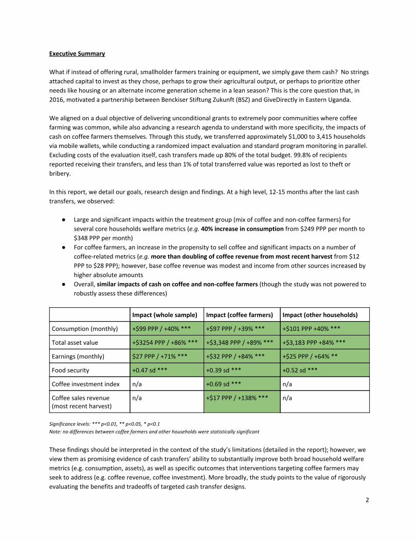
In this report, we detail our goals, research design and findings. At a high level, 12-15 months after the last cash

transfers, we observed:

● Large and significant impacts within the treatment group (mix of coffee and non-coffee farmers) for

several core households welfare metrics ( e.g. 40% increase in consumption from $249 PPP per month to

$348 PPP per month)

● For coffee farmers, an increase in the propensity to sell coffee and significant impacts on a number of

coffee-related metrics ( e.g. more than doubling of coffee revenue from most recent harvest from $12

PPP to $28 PPP); however, base coffee revenue was modest and income from other sources increased by

higher absolute amounts

● Overall, similar impacts of cash on coffee and non-coffee farmers (though the study was not powered to

robustly assess these differences)

Impact (whole sample) Impact (coffee farmers) Impact (other households)

Consumption (monthly) +$99 PPP / +40% *** +$97 PPP / +39% *** +$101 PPP +40% ***

Total asset value +$3254 PPP / +86% *** +$3,348 PPP / +89% *** +$3,183 PPP +84% ***

Earnings (monthly) $27 PPP / +71% *** +$32 PPP / +84% *** +$25 PPP / +64% **

Food security +0.47 sd *** +0.39 sd *** +0.52 sd ***

Coffee investment index n/a +0.69 sd *** n/a

Coffee sales revenue (most recent harvest)

n/a +$17 PPP / +138% *** n/a

Significance levels: *** p<0.01, ** p<0.05, * p<0.1

Note: no differences between coffee farmers and other households were statistically significant

These findings should be interpreted in the context of the study’s limitations (detailed in the report); however, we

view them as promising evidence of cash transfers’ ability to substantially improve both broad household welfare

metrics (e.g. consumption, assets), as well as specific outcomes that interventions targeting coffee farmers may

seek to address (e.g. coffee revenue, coffee investment). More broadly, the study points to the value of rigorously

evaluating the benefits and tradeoffs of targeted cash transfer designs.

2

I. Context and motivation

To date, decision-making in the aid industry has been dominated by the preferences and priorities of donors and

implementing organizations. Direct cash transfers flip the paradigm by putting resources directly in the hands of

recipients, and in doing so, empowering them to choose how best to address their own challenges. Beyond

conferring a high degree of agency to the “end user”, cash transfers have been shown to be a highly effective tool

for addressing many facets of poverty.

In 2016, the Overseas Development Institute conducted a large-scale review of the cash evidence, including 165

experimental or quasi-experimental studies from around the world. They found that cash transfers delivered a

wide range of positive outcomes, including economic development, improved health and nutrition, better school

attendance and psychological well-being. The study concluded that “the evidence on the impact of cash transfers

on poverty outcomes shows an overwhelmingly positive picture.” 1

Still, much remains to be learned about the results of varying cash transfer program designs, including the impact

and trade-offs associated with targeting various sub-populations. To develop a richer picture, studies are required

that recruit large samples of those sub-populations and measure a variety of outcomes. Against this backdrop, we 2

partnered with Benckiser Stiftung Zukunft (BSZ) on an initiative to both deliver a well-tested intervention to

extremely poor households, and deepen our knowledge of how cash transfers interact with a specific

subpopulation: smallholder coffee farmers.

Africa has an estimated 6.8 million smallholder coffee farmers, more than half of them living on less than 3 dollars

a day. Organizations seeking to help these communities have traditionally focused on delivering ‘in-kind’ support, 3

such as agricultural inputs or training programs. Many of these interventions have yet to be tested, despite being

implemented at scale. Cash can serve as an important benchmark to compare these interventions against.

GiveDirectly’s partnership with BSZ was structured around three main objectives:

● Offer direct benefits and choice to extremely poor households in a coffee-growing region of Uganda

through the delivery of lump-sum cash transfers.

● Study the impact of cash transfers on smallholder coffee farmers, and thereby provide a clear benchmark

for what coffee farmers can achieve if simply given cash.

● Understand the extent to which impacts for coffee farmers, if material, are driven by coffee-specific

investments.

To answer these and other questions, we designed and implemented a cash program for the target population,

and collaborated with the research consultancy, IDinsight, to assess its impact via a randomized evaluation.

1 Bastagli et al, ODI, “ Cash Transfers: what does the evidence say?”, 2016, https://www.odi.org/sites/odi.org.uk/files/resource-documents/10749.pdf 2 Blattman et al, “Cash as Capital”, 2017 https://ssir.org/articles/entry/cash_as_capital 3 Enveritas presentation at ASIC Portland, “A Comprehensive Estimate of Global Coffee Farmer Populations by Origin”, 2018 https://www.dropbox.com/sh/4bimju36sxkjptc/AAAFA68rFwbSAI4n3yCHjeKra/Sustainability%2C%20Climate%20Change%20%26%20Labels/Comprehensive%20Estimate%20of%20Global%20Coffee%20Farmer%20Populations%20By%20Origin-%20David%20Browning.pdf?dl=0 ; report forthcoming

3

II. Program design and execution

Location. Uganda is home to 1.7 million coffee farmers and is one of the world’s foremost coffee producers; it 4

exported more coffee than any other African country in 2017. Iganga District, in the Busoga region of Eastern 5

Uganda, is situated at the intersection of high poverty rates and substantial coffee production. The Uganda Bureau

of Statistics (UBOS) reported in 2009 that 46.2% of Iganga households (a total of 307,387 individuals) lived below

the UBOS-defined poverty line. The 2014 census reported that 6.7% of Iganga households were engaged in coffee 6

production. 7

Target population. GiveDirectly enrolled 3,415 households in 44 villages across 4 sub-counties in Iganga District.

Households were targeted based on poverty, using an index relying on households’ land and asset ownership.

About 30% of recipients reported prior to transfers that they had harvested coffee in one of the two previous

harvest seasons.

Transfers. All eligible households received a transfer of 3,400,000 UGX, the equivalent of approximately $1,000 in

nominal terms ($2,828 PPP). We sent transfers in three installments over the course of four months:

● Month 1: 400,000 UGX (~$118)

● Month 2: 1,500,000 UGX (~$441)

● Month 4: 1,500,000 UGX (~$441)

The total payment was sized to match our standard lump-sum model, which has been shown experimentally to

generate wide-ranging benefits for extremely poor populations comparable to those in this study. Transfers were 8

sent via MTN Mobile Money, the largest mobile cash provider in Uganda, and a vendor with whom we have

extensive experience delivering cash at scale.

The roles of partners. This initiative involved a collaboration between three organizations:

● BSZ funded the program and research in its entirety, including transfers for the control group after

completion of the endline in 2018.

● GiveDirectly was responsible for the overall program design and execution, including household

enrollment, transfer delivery, and standard operational monitoring. In addition, GiveDirectly field officers

collected a light baseline and a detailed endline survey, and our staff wrote this final evaluation report.

● IDinsight and GiveDirectly collaborated on the design and implementation of the research study. IDinsight

formulated the targeting criteria and survey tool, trained research enumerators, ran data quality checks,

and conducted all analysis. The analyses generated by IDinsight that are specified in the Pre-Analysis Plan

are reproduced in full in Annex C. All supplementary analyses are available by following this link.

4 Uganda Coffee Development Authority, FactSheet, https://ugandacoffee.go.ug/fact-sheet 5 International Coffee Organization, Trade Statistics Data , http://www.ico.org/historical/1990%20onwards/PDF/2a-exports.pdf 6 Uganda Bureau of Statistics, Iganga District Statistical Abstract, 2009, https://www.ubos.org/onlinefiles/uploads/ubos/2009_HLG_%20Abstract_printed/Iganga%20District%20statistical%20abstract%202009.pdf 7 Uganda Bureau of Statistics, National Population and Housing Census - Area Specific Profiles: Iganga, 2017, https://www.ubos.org/wp-content/uploads/publications/2014CensusProfiles/IGANGA.pdf 8 Haushofer, J., & Shapiro, J. (2016). The Short-Term Impact of Unconditional Cash Transfers to the Poor: Experimental Evidence from Kenya. The Quarterly Journal of Economics 131(4), 1973–2042

4

III. Methods

Study methods were pre-specified in the Pre-Analysis Plan published on the RIDIE research registry prior to any

analysis of endline data. They are summarized below and presented in detail in Annex A. 9

Study sample . The study took place in 44 villages across 4 sub-counties in Iganga District. The poorest 20% of

households in the study villages were automatically considered eligible to receive cash transfers and excluded from

the sample. The wealthiest 36% of households were deemed ineligible and also excluded.

3,788 households between the 20th and 64th percentiles were included in the study and randomized to treatment

(n=1,894) or control (n=1,894) groups, using matched pair randomization based on their ownership of coffee trees

and level of coffee production.

Study design. The majority of experimental research on cash finds impacts across a wide range of benefits, an

unsurprising result given the inherent flexibility of the intervention. Given constraints on survey length, we chose

to focus the limited budget for this study on (1) coffee outcomes and (2) a subset of household welfare outcomes

variables where significant impacts were found in an earlier study of GiveDirectly transfers. We did not consider 10

temptation goods as a separate outcome, due to overwhelming evidence that cash does not cause

disproportionate increases in vice spending. The outcome variables measured for all study households were 11

bucketed in two main categories:

● Household welfare, for which we collected data on:

○ Total household consumption

○ Total asset value

○ Agricultural and business earnings

○ Food security index

● Coffee-specific outcomes, for which we collected data on:

○ Coffee investment index

○ Revenue from coffee sales

Assuming 80% power and a significance level of 5%, the estimated minimum detectable effect size for outcomes

applying to the entire sample was 0.09, and 0.16 for outcomes applying only to coffee farmers.

Data collection. A light baseline survey containing questions relating to targeting criteria as well as recent

experience with coffee farming was conducted at the outset, and a detailed endline survey approximately 18

months later. The time period between the final payment to recipients and the endline was 12-15 months. We set

the timing of the endline to ensure we were collecting data at the point in the agricultural cycle where coffee had

been harvested by farmers.

GiveDirectly field officers collected data through enumerator-administered in-person surveys designed by

IDinsight. A number of steps were taken to maximize the quality of data collected, including (1) extensive piloting

9 http://ridie.3ieimpact.org/index.php?r=search/detailView&id=521 10 Haushofer, J., & Shapiro, J. (2016). The Short-Term Impact of Unconditional Cash Transfers to the Poor: Experimental Evidence from Kenya. The Quarterly Journal of Economics 131(4), 1973–2042 11 Evans, D. & Popova, A. (2014). Cash transfers and temptation goods : a review of global evidence. Policy Research working paper ; no. WPS 6886; Impact Evaluation series ; no. IE 127. Washington, DC: World Bank Group.

5

(2) rigorous training for GD enumerators from IDinsight staff, and (3) data checks regularly administered by

IDinsight for consistency and qualit y. We provide further detail on these processes in Annex F.

IV. Findings

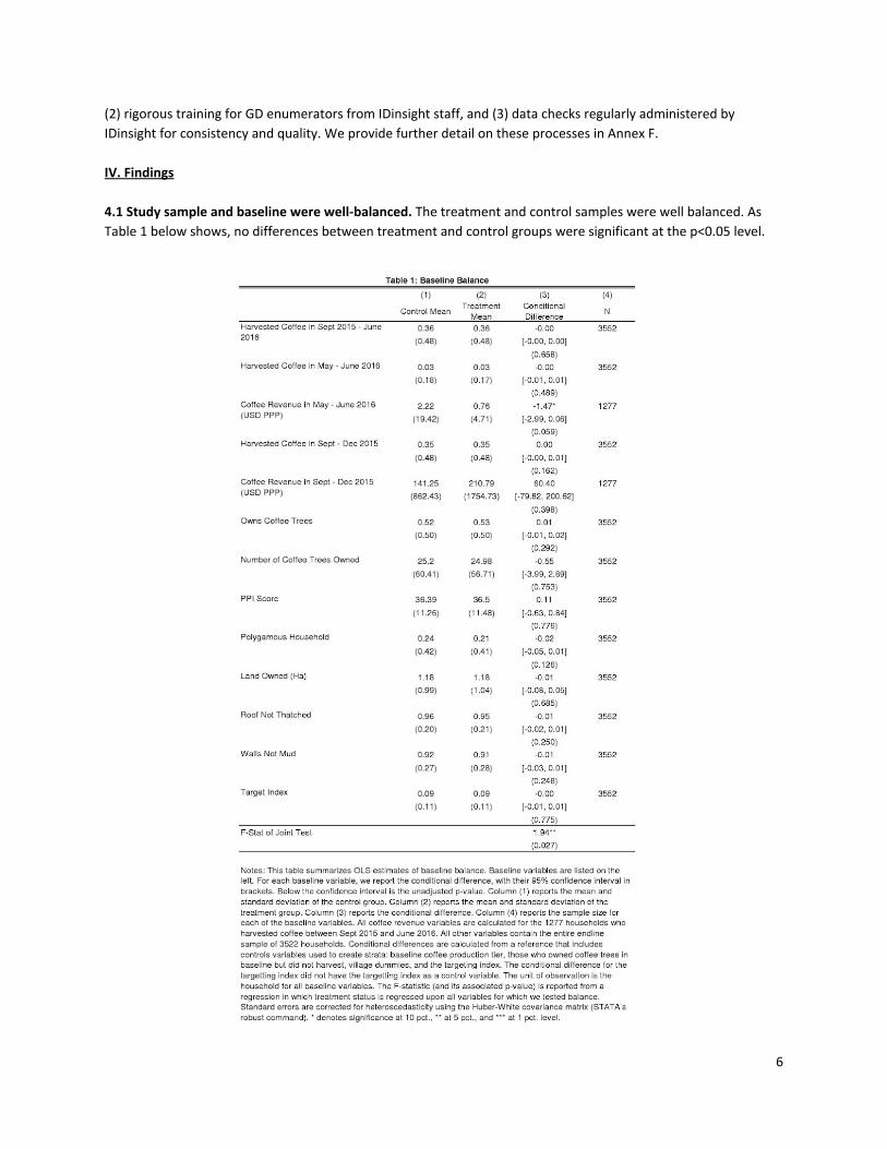
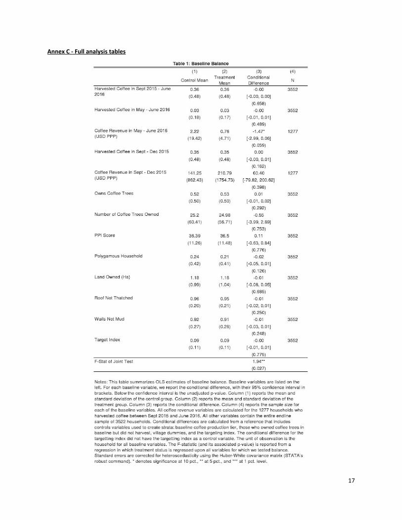
4.1 Study sample and baseline were well-balanced. The treatment and control samples were well balanced. As

Table 1 below shows, no differences between treatment and control groups were significant at the p<0.05 level.

6

4.2 The study sample was predominantly poor, and coffee farmers had multiple income sources. While we

excluded the poorest 20% of households from the study, those who participated were still very poor. Household

consumption for controls averaged $249 PPP per month, or $1.89 PPP per day per household member - just $0.67

per day in nominal terms. Monthly agricultural and business revenue for controls averaged $65 PPP per month,

excluding coffee income.

Coffee farmers represented 36% of the sample and were classified as households who grew and harvested coffee

in either of the prior two seasons before baseline. Revenue from coffee sales during the most recent harvest was

modest and averaged $12 PPP for coffee farmers in the control group, around $2 PPP per month assuming two

harvests per year. Further analyses found that only 45% of baseline coffee farmers in the control group reported

any coffee sales in the most recent harvest.

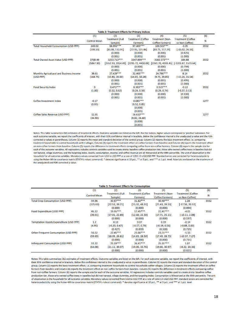
4.3 Household welfare metrics increased across the board. Cash transfers of ~1,000 USD ($2,829 PPP) had large

impacts on all measures of household welfare 18 months after baseline, and 12-15 months after final transfers

were received. Detailed results are presented in Table 2 and below, we synthesize key findings, including how

results compared to an earlier study on GiveDirectly’s lump-sum program in Rarieda, Kenya.

7

● Total consumption increased by 40% (from a base of $249 PPP per month), with expenditure on food

rising by 44% and consumption of crops grown by the household increasing by 33%. This finding is broadly

in line with the impact of $1,000 transfers in the Rarieda RCT, where consumption increased by 32% nine

months after baseline. 12

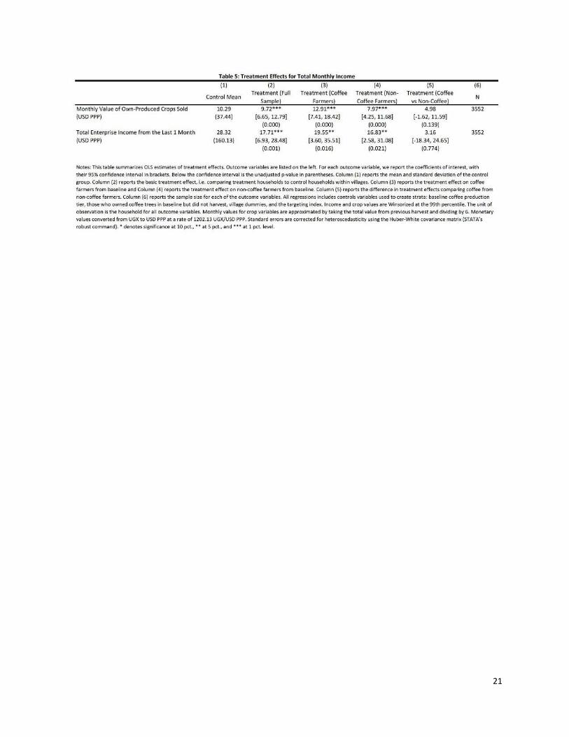
● Earnings rose considerably for the treatment group: up 71% overall, including an increase in enterprise

earnings of 63% and a growth in non-coffee crop sales of 94% (driven largely by increased sales of rice and

maize). In the Rarieda study, earnings increased by 29% for households that received $1,000 transfers.

Supplementary analyses showed that the increase in enterprise revenue was driven by households

starting new enterprises, as opposed to growing the revenue of existing enterprises.

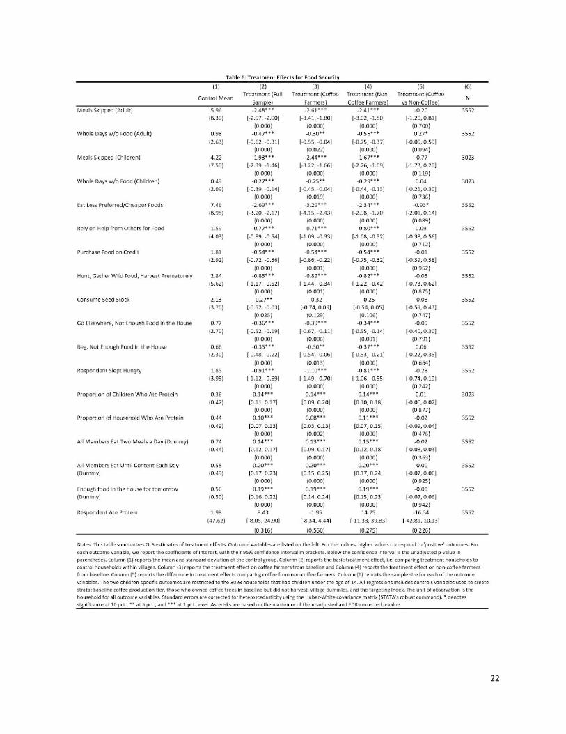
● Food security improved markedly. An index measure increased by 0.47 standard deviations, including a

46% decrease in child meals skipped, a 42% decrease in adult meals skipped and a 39% increase in the

proportion of children who ate protein. These findings are broadly in line with the changes in food

security in the Rarieda study, where $1,000 transfers increased scores on the same food security index by

0.39 standard deviations.

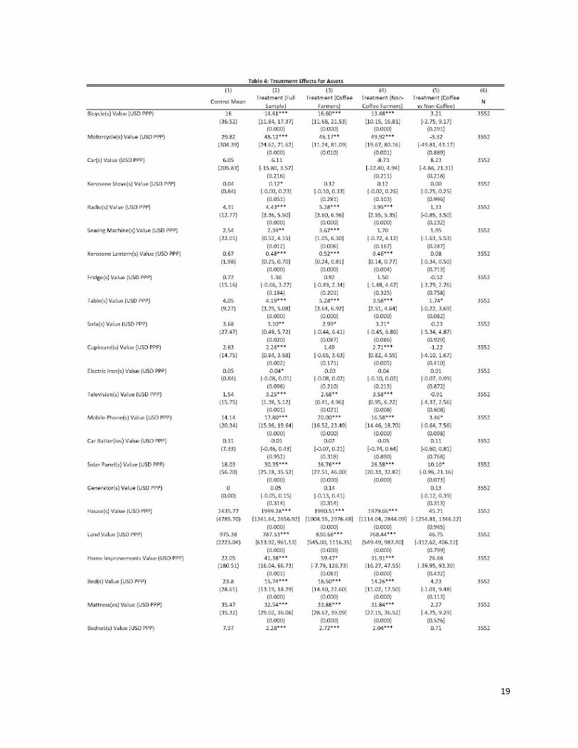
● The total value of assets increased by 86% ― livestock values tripled, the value of land owned increased

by 81% , and house values increased by 82%. The increase in livestock value was higher in relative 13 14

terms in this study (+200%) than for $1,000 transfers in the Rarieda study (+78%), though in absolute

terms the increase per $1,000 PPP transferred was broadly similar (+$74 vs +$85 for Rarieda). Smaller, but

statistically significant, increases were recorded for a range of asset types from mattresses to bed nets to

solar panels to bicycles, illustrating the broad range of goods that recipients purchased (see table 4 in

Annex C for full details).

In summary, cash transfers meaningfully increased household spending (including on food), increased earnings,

improved food security, and led households to increase their assets. With respect to the last category, we are

more plausibly able to explain and/or benchmark some dimensions of asset growth than others, which begs

further study.

4.4 Coffee investment and revenue increased, though total earnings gain was driven more by non-coffee

sources.

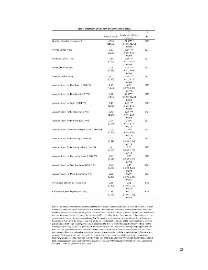
We observe a large (0.69 standard deviations) increase in the index measure of coffee investment by coffee

farmers. Unpacking the measures that compromise that index, households that received transfers increased their

adoption rate of recommended agricultural practices including pruning (+25%), stumping (+47%), mulching (+100%

from a low base) and weeding (+23%) coffee trees. Spending on new land, sacks, pesticide, fertilizer, and coffee

transportation all rose. However, with the exception of new land (+$56 PPP), these statistically significant changes

12 See table 69, column 2 of the Haushofer & Shapiro (2016) online appendix https://www.princeton.edu/~joha/publications/Haushofer_Shapiro_UCT_Online_Appendix.pdf 13 Additional land value analyses by IDinsight suggest two main drivers: (i) a 57% increase in the area of land owned (from 0.14 ha to 0.22ha), and (ii) a 29% increase in the perceived value of each hectare of land land. Farmers may have purchased higher-value land, or the treatment could have caused farmers to value their land more highly (possibly because it had become more productive). 14 The large increases in self-assessed house value ($2,040 PPP, 72% of the transfer) in particular are difficult to explain and puzzling. The difference between treatment and control spending on home improvements was $41 PPP (see table 4 in Annex C), which is only 2% of the reported change in house value. Asset value questions were framed as the amount that respondents would be willing to sell the asset for. It seems possible that treated households, for some reason, were less willing than controls to sell their houses in this hypothetical scenario..

8

were small in absolute magnitude: all were under $1 PPP per coffee farming household (see Annex C, table 7 for

full details). It therefore appears that coffee farming households chose to spend the majority of their cash transfers

on investments that were not coffee-specific.

As set out in section 4.2, coffee sales made up a relatively small proportion of total household revenue from

agriculture and enterprise for control coffee farmers. On average, control coffee farmers owned 47 coffee trees,

fewer than ~290 trees that the typical Uganda coffee farmer owns. Cash transfers more than doubled coffee 15

sales revenue from the most recent harvest ― an increase of 138% (+$17 PPP). Some of this increase appears to

have been driven by a 62% increase in the number of coffee trees owned (likely through purchasing land with

mature coffee trees) and achieving a slightly higher price for their coffee ($0.73 PPP per kg vs $0.66 PPP for

controls, significant at the 10% level). Supplementary analyses by IDinsight suggested that cash transfers increased

the propensity to sell coffee, through a combination of more households switching to become coffee farmers, and

fewer households ceasing to cultivate coffee less often (54% of coffee farmers who received transfers sold coffee

at endline, compared to 45% for control coffee farmers). Supplementary analyses also suggested that treatment

effects were largest, in both relative and absolute terms, for coffee farmers in the top third of baseline coffee

production.

One challenge we hypothesized cash transfers might address is the picking of unripe coffee cherries when

resources are tight. However, the data show that picking unripe cherries is not an issue for the study villages: 98%

of control and 99% of treatment coffee farmers reported picking cherries only when they were ripe. Rather, the

increase in coffee revenue appears to be driven by an increase in production volume ― cash transfers led to a 62%

increase in the number of coffee trees owned and an increased propensity to harvest coffee.

Cash transfers also generated earnings gains from non-coffee sources. Enterprise income per month was 63%

higher (+$20 PPP per month, +$235 on an annualized basis) for coffee farmers who received a cash transfer than

for controls. Sales of own-produced crops were 94% higher (+$13PPP per month, +$155 on an annualized basis).

These increases in earnings were much higher, in absolute terms, from non-coffee sources than from coffee

revenue (which increased by around $3 PPP per month, +$33 PPP on annualized basis). Supplementary analyses by

IDinsight calculated that the average proportion of income from coffee was 6.8% for households that harvested 16

coffee at baseline, and 13.7% for those who also harvested coffee at endline.

As noted in the methods section, the study was not well powered to detect differences between impacts on coffee

farmers and other households. That said, we found the impacts of cash transfers on household welfare to be

similarly positive for households who farm coffee and those who do not. Consumption increased by 39% in coffee

farming households (vs 40% for other households), and assets increased by 89% (vs 84%). Agricultural and business

income changes were directionally higher for coffee farmers (+84% vs +64%), but food security gains were

directionally slightly lower (+.39 sd vs +.51 sd).

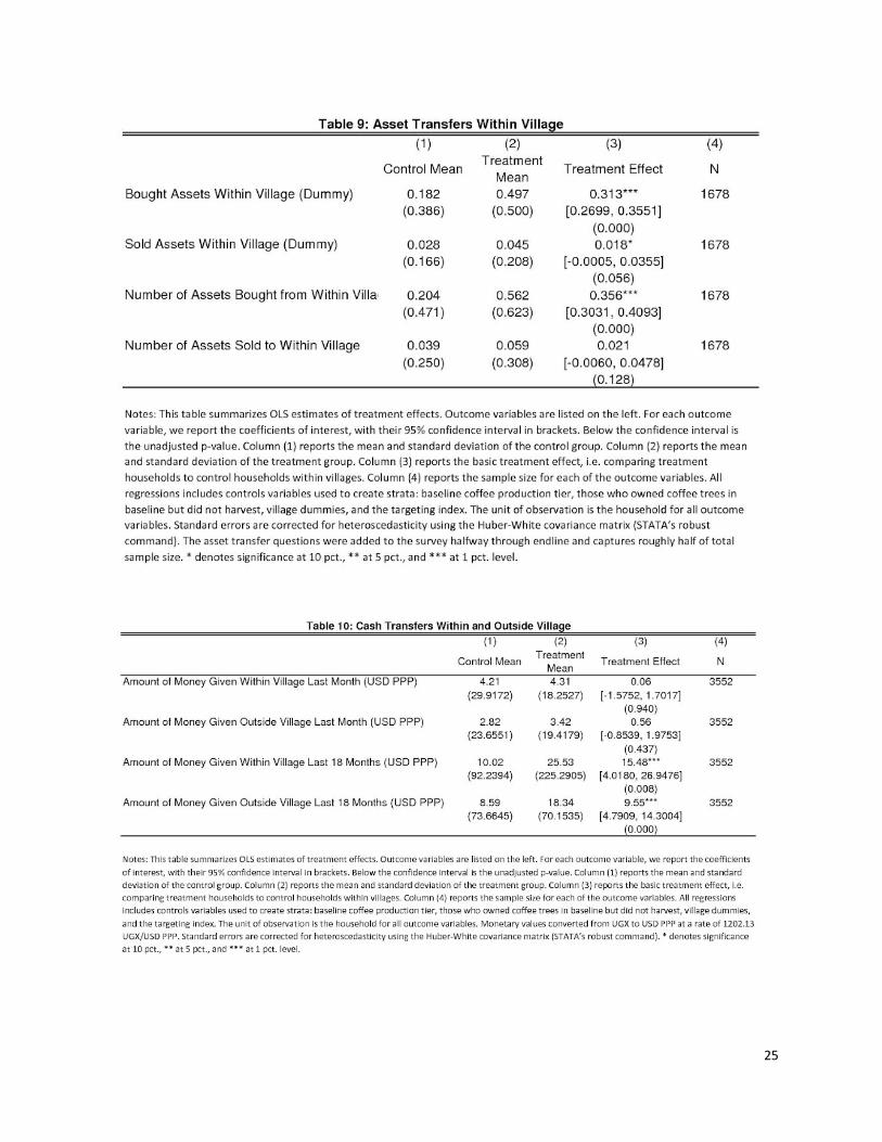
4.5 Recipients used transfers for their own households’ spending.

A small proportion (under 1%) of the total value of cash transfers was transferred onward by recipients to other

households. As table 10 shows (see Annex C), treatment households on average gave more money within the

15 Enveritas presentation at ASIC Portland, “A Comprehensive Estimate of Global Coffee Farmer Populations by Origin”, 2018 https://www.dropbox.com/sh/4bimju36sxkjptc/AAAFA68rFwbSAI4n3yCHjeKra/Sustainability%2C%20Climate%20Change%20%26%20Labels/Comprehensive%20Estimate%20of%20Global%20Coffee%20Farmer%20Populations%20By%20Origin-%20David%20Browning.pdf?dl=0 ; report forthcoming 16 This is the average of the ratios for individual farmers.

9

village than did controls in the last 18 months (+$15 PPP, about 0.5% of transfer value), as well as more money

outside the village (+$10 PPP, 0.3% of transfer value).

4.6 Study limitations

The study design has some limitations, which should be taken into account when interpreting results.

(i) Randomization approach

The large size of villages in the Iganga region of Uganda meant that the study could not achieve sufficient statistical

power with a village level randomization. In consultation with IDinsight, we decided to implement randomization

at the individual household level instead. While this approach delivered high statistical power, it also carried

limitations. Without a ‘pure’ control group (study villages where no household receives cash), it is not possible to

directly measure the extent to which differences between treatment and control households reflect

treatment-induced changes in welfare versus ‘spillover’ effects (where outcomes for control households are

better/worse than they would otherwise have been, for example due to changes in the price of goods or changes

in the amount of demand in the village economy). It’s worth noting that a large-scale RCT of GiveDirectly’s

program (called the General Equilibrium study ) will provide robust results on the extent to which $1,000 cash 17

transfers generate positive or negative spillover effects (to be published in mid-2019).

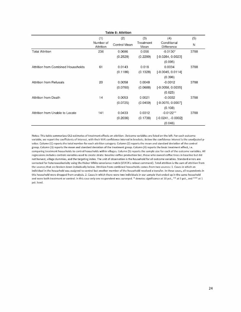
We did attempt to measure spillover impacts indirectly by asking both treatment and control households whether

they had, in the last two years, sold assets to others in the village, and/or had purchased assets from others in the

village (see Annex C, table 9 for detail). This was motivated by the findings of a recent study of the longer-term

effects of GiveDirectly’s Rarieda program, which found some indications of negative spillovers for within-village

control households. The authors of that study speculated that this effect may have been caused by control 18

households selling productive assets to households who received transfers. These findings were released part-way

through the endline survey, and as a result the additional questions were only collected for part of the sample.

Overall, the limited data collected in the present study does not explicitly support that hypothesis. Patterns of

asset sales were broadly similar across treatment and control households (see Annex C, Table 9), and there was no

category where controls reported selling more assets within the village than did treatment households. Treatment

households did, however, buy more assets within the village (largely mobile phones). Although our exploratory 19

analysis did not find convincing evidence of asset transfer spillovers, we are unable to definitively rule out the

hypothesis that the large estimated treatment effect on assets was in part generated by within-village asset

transfers from treatment to control. Other mechanisms through which spillover impacts could operate, such as

prices, were not measured in this study. Preliminary results from a the General Equilibrium study suggest no

impact on prices, no negative spillovers and slightly positive spillovers for consumption and psychological

wellbeing . 20

(ii) GiveDirectly’s role in the evaluation

17 General Equilibrium study AEA Trial Registry entry https://www.socialscienceregistry.org/trials/505 18 Haushofer, J., & Shapiro, J. (2018). The Long-Term Impact of Unconditional Cash Transfers: Experimental Evidence From Kenya 19 Further analysis of asset sales and purchases with villages can be found at Annex D 20 https://www.givewell.org/international/technical/programs/cash-transfers/spillovers

10

To minimize data collection costs, baseline and endline data were collected by GiveDirectly staff. Several steps

were taken to ensure that a high standard was met for data collection ( e.g. enumerators received extensive

in-person training from IDinsight, the quality of survey data was monitored daily by IDinsight, and independent

back-checks were run to triangulate data quality).

Nevertheless, it remains possible that self-reported measures could be more biased. For instance, grateful

recipients may have been inclined to report what they thought enumerator wanted to hear. In the opposite

direction, controls may have understated their welfare in the hopes of receiving a transfer in the future. While

recent work suggests that the extent to which these biases could drive survey responses is modest , our findings 21

should be interpreted with due caution.

V. Operational performance

5.1 Operational efficiency was robust, though lower than standard GD programming due to research design

The all-in efficiency of the program, including evaluation cost, was 74%. In other words for every $1 of the

Benckiser Stiftung Zukunft’s investment, $0.74 was transferred directly to a recipient. Excluding the cost of the

evaluation, which allows for a more accurate measure of the cost per dollar delivered, our operational efficiency

increases to 80% (see Annex B for more detail). The lower efficiency of this program relative to our standard

operations was in line with expectations, given the cost (including field staff and management time) of delivering a

more complex targeting and randomization design.

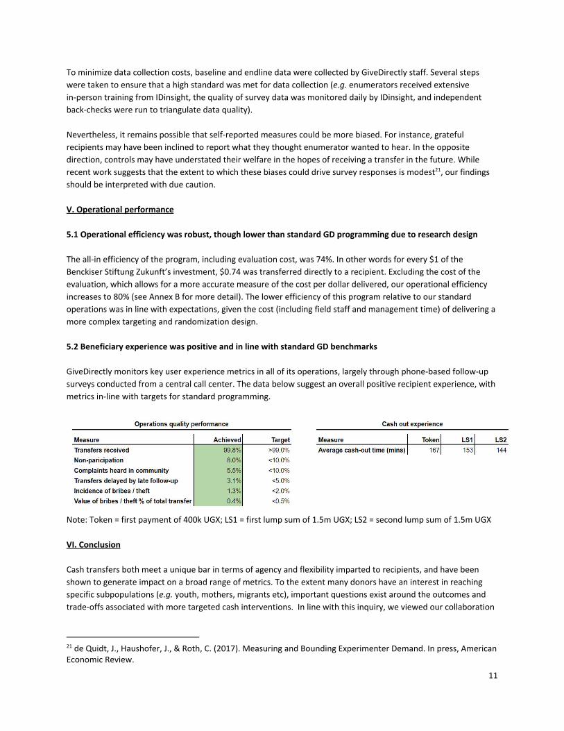
5.2 Beneficiary experience was positive and in line with standard GD benchmarks

GiveDirectly monitors key user experience metrics in all of its operations, largely through phone-based follow-up

surveys conducted from a central call center. The data below suggest an overall positive recipient experience, with

metrics in-line with targets for standard programming.

Note: Token = first payment of 400k UGX; LS1 = first lump sum of 1.5m UGX; LS2 = second lump sum of 1.5m UGX

VI. Conclusion

Cash transfers both meet a unique bar in terms of agency and flexibility imparted to recipients, and have been

shown to generate impact on a broad range of metrics. To the extent many donors have an interest in reaching

specific subpopulations ( e.g. youth, mothers, migrants etc), important questions exist around the outcomes and

trade-offs associated with more targeted cash interventions. In line with this inquiry, we viewed our collaboration

21 de Quidt, J., Haushofer, J., & Roth, C. (2017). Measuring and Bounding Experimenter Demand. In press, American Economic Review.

11

with BSZ as a both a vehicle for delivering value to extremely poor households, and for advancing the literature on

cash in the context of a specific but consequential community. In the course of this study, we learned that:

● Populations with high concentrations of coffee farmers, like other extremely poor communities given

cash, experienced broad and significant improvements in assets, consumption, and food security more

than a year after transfers were made.

● Moreover, despite the inherently diffuse nature of cash impacts, improvements materialized for narrow

outcomes typically targeted by customized, in-kind interventions ( e.g. adoption of positive agricultural

practices such as pruning, stumping, mulching and weeding of coffee trees, as well as increases in coffee

investments and revenue).

● Importantly, the considerable increase in earnings experienced by coffee farmers was more driven by

non-coffee sources, underscoring the value of giving recipients flexibility to allocate funds in the manner

they deem most productive.

The above findings represent an exciting starting point. That said, given design limitations of this study and the

narrow set of outcomes assessed, we recommend further investigation of a number of questions:

● What role does coffee farming play in the livelihoods portfolio of poor coffee farmers?

● How are smallholder farmers making trade-offs across different investment options when give a cash

infusion?

● Are there behavior nudges or other “plus” component that might cheaply amplify the impact of cash in

this population?

● What are the longer-term effects of cash transfers on coffee farmers?

We look forward to either pursuing these questions ourselves, or seeing others in the space advance our

understanding of this population and the potential for cash to be impactful within it.

12

Annex A - Study methods (detail)

Sampling: This study adhered to GiveDirectly’s standard approach to targeting and enrollment, with slight

adjustments.

Assignment method: Eligible households were assigned to the treatment and control groups using matched pair

randomization. Households were first grouped into coffee-growers and non-coffee producers (within the previous

year). Coffee growers were additionally grouped into “high production”, “medium production,” and “low

production,” based on their tercile for the amount of coffee sold during the most recent main coffee season.

Non-coffee producers were divided into two groups: those who owned coffee trees and those who didn’t. Within

each group, households were then sorted by the value of the targeting index, and matched with their nearest

neighbor. Within each pair, one household was randomly assigned to treatment, and one to control.

Randomization was conducted using STATA.

Power : Across the 3,788 households in the sample, 1,894 households were in the treatment arm and 1,894 in the

control arm. 1,351 households grew coffee the previous year (677 in the treatment arm and 674 control in the

control arm). Assuming 80% power and a significance level of 0.05, the minimum detectable effect size (MDES),

0.09 standard deviations for outcomes that apply to the entire sample. For outcomes that apply only to coffee

farmers, the MDES was 0.16. Based on the results of previous studies such as Haushofer and Shapiro (2016) , this 22

was well within the range of expected effects. To compare effects of coffee farmers to non-coffee farmers, the

MDES is .14. However, we expected differential effects between these two groups to be quite small, so we did not

expect to be powered for this analysis.

22 Haushofer, J., & Shapiro, J. (2016). The Short-Term Impact of Unconditional Cash Transfers to the Poor: Experimental Evidence from Kenya. The Quarterly Journal of Economics 131(4), 1973–2042

13

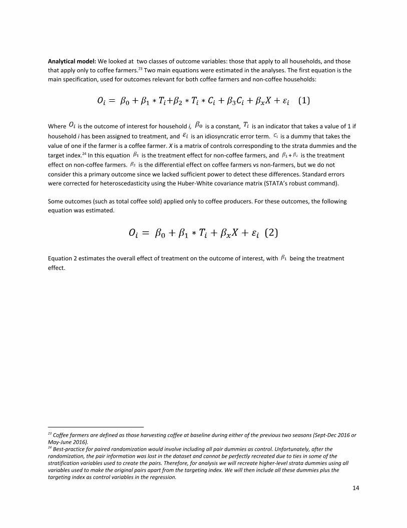
Analytical model: We looked at two classes of outcome variables: those that apply to all households, and those

that apply only to coffee farmers. Two main equations were estimated in the analyses. The first equation is the 23

main specification, used for outcomes relevant for both coffee farmers and non-coffee households:

Where is the outcome of interest for household i, is a constant, is an indicator that takes a value of 1 if

household i has been assigned to treatment, and is an idiosyncratic error term. is a dummy that takes the

value of one if the farmer is a coffee farmer. X is a matrix of controls corresponding to the strata dummies and the

target index. In this equation is the treatment effect for non-coffee farmers, and + is the treatment 24

effect on non-coffee farmers. is the differential effect on coffee farmers vs non-farmers, but we do not

consider this a primary outcome since we lacked sufficient power to detect these differences. Standard errors

were corrected for heteroscedasticity using the Huber-White covariance matrix (STATA’s robust command).

Some outcomes (such as total coffee sold) applied only to coffee producers. For these outcomes, the following

equation was estimated.

Equation 2 estimates the overall effect of treatment on the outcome of interest, with being the treatment

effect.

23 Coffee farmers are defined as those harvesting coffee at baseline during either of the previous two seasons (Sept-Dec 2016 or May-June 2016). 24 Best-practice for paired randomization would involve including all pair dummies as control. Unfortunately, after the randomization, the pair information was lost in the dataset and cannot be perfectly recreated due to ties in some of the stratification variables used to create the pairs. Therefore, for analysis we will recreate higher-level strata dummies using all variables used to make the original pairs apart from the targeting index. We will then include all these dummies plus the targeting index as control variables in the regression.

14

Annex B - Efficiency calculations (detail)

Costs and efficiency: GiveDirectly categorizes its costs in two main buckets: (1) the value of cash transfers

delivered to recipients (2) all costs associated with delivering the cash transfers, including direct costs (personnel,

travel, telcom fees etc) and an allocation of organization-wide costs that the program bears. GiveDirectly reports

its operational efficiency simply as the proportion of the overall budget that is transferred directly to recipients,

where overall budget is the sum of categories (1) and (2) above.

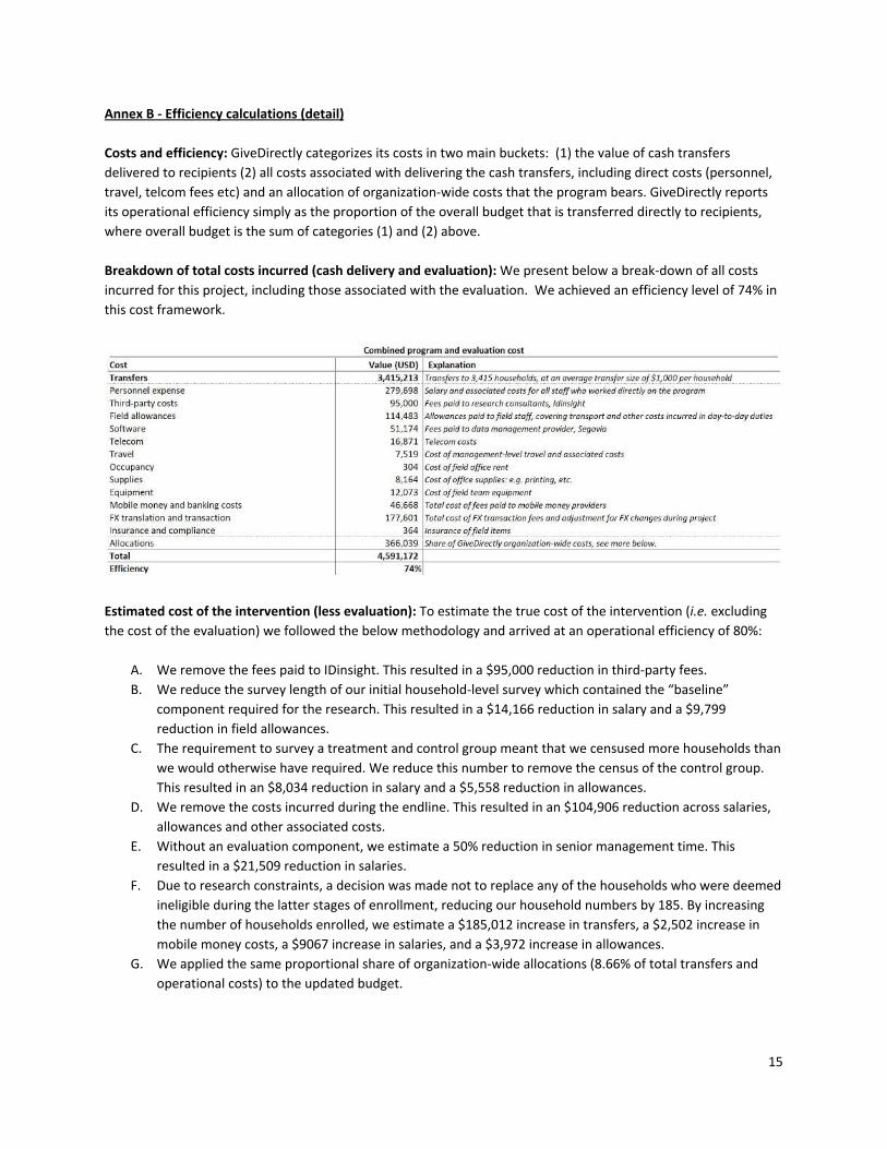
Breakdown of total costs incurred (cash delivery and evaluation): We present below a break-down of all costs

incurred for this project, including those associated with the evaluation. We achieved an efficiency level of 74% in

this cost framework.

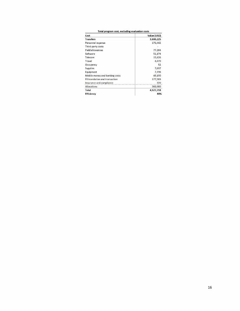
Estimated cost of the intervention (less evaluation): To estimate the true cost of the intervention ( i.e. excluding

the cost of the evaluation) we followed the below methodology and arrived at an operational efficiency of 80%:

A. We remove the fees paid to IDinsight. This resulted in a $95,000 reduction in third-party fees.

B. We reduce the survey length of our initial household-level survey which contained the “baseline”

component required for the research. This resulted in a $14,166 reduction in salary and a $9,799

reduction in field allowances.

C. The requirement to survey a treatment and control group meant that we censused more households than

we would otherwise have required. We reduce this number to remove the census of the control group.

This resulted in an $8,034 reduction in salary and a $5,558 reduction in allowances.

D. We remove the costs incurred during the endline. This resulted in an $104,906 reduction across salaries,

allowances and other associated costs.

E. Without an evaluation component, we estimate a 50% reduction in senior management time. This

resulted in a $21,509 reduction in salaries.

F. Due to research constraints, a decision was made not to replace any of the households who were deemed

ineligible during the latter stages of enrollment, reducing our household numbers by 185. By increasing

the number of households enrolled, we estimate a $185,012 increase in transfers, a $2,502 increase in

mobile money costs, a $9067 increase in salaries, and a $3,972 increase in allowances.

G. We applied the same proportional share of organization-wide allocations (8.66% of total transfers and

operational costs) to the updated budget.

15

16

Annex C - Full analysis tables

17

18

19

20

21

22

23

24

25

Annex D - Asset purchases and sales within study villages

The overall proportion of households that sold assets was slightly higher for treatment (4.5%) than for control

(2.8%) households, significant at the 10% level. This appears to be driven by treatment households selling more

chickens within the village than control households (results available upon request).

Asset purchases within the village represented a more complex story. Treatment households did buy more assets

overall. This difference was largely driven by treatment households buying more mobile phones (44% vs 16%), with

a small contribution from other asset categories: bicycles (4% vs 2%) and sewing machines (1% vs 0%). While the

questions specified purchases from an individual within the village, it is plausible that the large-scale sale of mobile

phones by GiveDirectly (98% of recipients chose to purchase) could have accounted for some of the reported

difference. Treated households bought 0.35 more assets per household in total within the villages than controls,

but only 0.07 more when mobile phones are excluded.

One potential driver of the large change in land value reported in table 4 (Annex C) is treatment households

purchasing land from control households. However, there was little reported trading of land within the village. Less

than 1% of the treatment sample reported buying land within the village, and less than 0.1% of controls reported

selling land within the village. While the difference between land purchase rates was significant (0.8% for

treatment vs 0.1% for controls), this seems unlikely to account for the doubling of land value overall for treatment

households. It is possible that treatment households could have purchased land from outside the village, or could

be assigning higher value to the land they own.

26

Annex E - Composition of index outcome variables

1. Total household consumption : 25

A. Food expenditure

B. Value of own-produced food consumed

C. Temptation good expenditure (tobacco, alcohol, and other intoxicants)

D. Other frequent consumption (fuel, transport, entertainment, airtime, personal care, etc.)

E. Infrequent consumption (medical, education, assets, etc.)

2. Total estimated value of owned assets:

A. Bicycle

B. Motorcycle/scooter

C. Car/truck

D. Kerosene stove

E. Radio/cassette player/CD player

F. Sewing machine

G. Kerosene Lantern

H. Bed

I. Mattress

J. Bednet

K. Fridge and/or Freezer

L. Pots and Pans

M. Tables

N. Sofa pieces

O. Chair

P. Cupboards/dressers

Q. Clock or Watch

R. Electric Iron

S. Television

T. Mobile Phone

U. Car Battery

V. Hoes

W. Pangas

X. Slashers

Y. Hand Cart

Z. Wheelbarrow

AA. Ox plow

BB. Solar panel

CC. Generator

DD. Livestock (chickens, goats, cattle, pigs, other)

EE. House

FF. Land

GG. Home improvements

HH. Plates

II. Cleaning tools

25 To avoid capturing opposing effects, the consumption index does not include flow spending on durables, such as roof repair. These types of spending could go down as a result of buying new assets.

27

JJ. Roof is not thatched*

KK. Walls are not earth/mud*

LL. Floor is not earth/mud*

MM. House has toilet or pit latrine*

*Outcomes with an asterisk were studied but not included in the asset total as they are binary indicators.

For polygamous households in which an asset was reported as shared among the wives, each individual wife was

given an allocation (total value of asset/number of wives).

3. Monthly agricultural and business income

A. Total value of production of major crops, scaled to monthly figure (own-consumed) 26

B. Total value of production of major crops, scaled to monthly figure (sold)

C. Non-farm enterprise revenue (in the last 1 month)

4. Food Security Index (same as Haushofer and Shapiro 2016)

A. Meals skipped (adults and children)

B. Whole days without food (adults and children)

C. Eat less preferred/cheaper foods

D. Rely on help from others for food

E. Purchase food on credit

F. Hunt, gather wild food, harvest prematurely

G. Beg because not enough food in the house

H. All members eat two meals

I. All members eat until content

J. Number of times ate meat or fish

K. Enough food in the house for tomorrow?

L. Respondent slept hungry

M. Respondent ate protein

N. Proportion of household who ate protein

O. Proportion of children who ate protein

5. Coffee Investment Index

A. Number of coffee trees owned/land dedicated to coffee

B. Respondent stumped (rehabilitated) coffee trees

C. Respondent pruned coffee trees

D. Amount spent on hired labor for coffee

E. Amount spent processing/transporting coffee

F. Amount spent on other coffee inputs

G. Percentage of cherries sold that were picked once ripe (percentage of cherries that were picked

red as opposed to green)

H. Coffee price per kilogram

6. Revenue from coffee sales - no component indicators

26 Our survey asks about harvest and sales from the most recent harvest season. Given that there are two harvest seasons for most crops in the regions, we convert to an approximate monthly figure by dividing by 6.

28

Annex F - Enumerator training and data monitoring

Training

IDInsight conducted two weeks of classroom training, and additional training in the field ( i.e. dry runs). The main

goals of the training were around:

● Best practices: (1) Emphasizing general enumeration concepts, including guidelines for interviews ( i.e.

neutral probing, attentive listening, etc). (2) Identifying escalation scenarios for engaging supervisors. (3)

Mastering the SurveyCTO platform on a mobile phone.

● Content: (1) Training on the complex protocols such as respondent identification and relocations. (2)

Thoroughly explaining the higher-complexity crop, coffee, asset, consumption, enterprise, and food

security modules of the survey. (3) Reviewing the protocols in Busoga with role playing.

● Experience : Piloting the survey in the field to provide opportunities for iteration and feedback.

For the asset module, IDinsight trained enumerators to collect the number and value of owned assets. The asset

had to be fully functional and considered a possession of the household. Enumerators were trained to frame the

estimated value as willingness to accept - i.e. the amount they were willing to sell the asset. House values included

the value of the land plot that the house was on. Land value consists of additional plots of land that the household

owns, often for agricultural purposes. For cases of multiple houses and land plots, respondents were asked to

estimate the total value. If respondents provided values for individual houses and plots, enumerators were trained

to add land values on their notepad or phones.

Data quality monitoring

IDInsight’s quality control protocols included:

● High frequency data checks: IDinsight ran weekly quality checks on data collected and sent a status report

to GiveDirectly. The weekly reports included number of surveys completed, whether the right

respondents had been surveyed, response rates and survey duration, flags on missing/suspect values, and

comparison of key variables against baseline data. Adjustments to the survey and/or additional

enumerator training were conducted case by case.

● Survey backchecks: IDinsight regularly backchecked completed surveys to triangulate quality. Specifically,

they selected ~10% of previously-surveyed households and re-asked those households a subset of the

original survey questions. The selection of surveys and enumerators was in part based on the results of

high frequency checks, particularly in cases where fraud or incompetence was suspected. Responses were

reconciled against the original GiveDirectly data; where required, underperforming field officers were

provided additional training or, in some cases, disciplinary action was applied.

29