case studies in using reliability performance measures in...

SHRP 2 Reliability Project L05

Case Studies in Using Reliability Performance Measures in Transportation Planning

SHRP 2 Reliability Project L05

Case Studies in Using Reliability Performance Measures in Transportation

Planning

Cambridge Systematics, Inc.

TRANSPORTATION RESEARCH BOARD Washington, D.C.

2014 www.TRB.org

© 2014 National Academy of Sciences. All rights reserved. ACKNOWLEDGMENT This work was sponsored by the Federal Highway Administration in cooperation with the American Association of State Highway and Transportation Officials. It was conducted in the second Strategic Highway Research Program, which is administered by the Transportation Research Board of the National Academies. COPYRIGHT INFORMATION Authors herein are responsible for the authenticity of their materials and for obtaining written permissions from publishers or persons who own the copyright to any previously published or copyrighted material used herein. The second Strategic Highway Research Program grants permission to reproduce material in this publication for classroom and not-for-profit purposes. Permission is given with the understanding that none of the material will be used to imply TRB, AASHTO, or FHWA endorsement of a particular product, method, or practice. It is expected that those reproducing material in this document for educational and not-for-profit purposes will give appropriate acknowledgment of the source of any reprinted or reproduced material. For other uses of the material, request permission from SHRP 2. NOTICE The project that is the subject of this document was a part of the second Strategic Highway Research Program, conducted by the Transportation Research Board with the approval of the Governing Board of the National Research Council. The Transportation Research Board of the National Academies, the National Research Council, and the sponsors of the second Strategic Highway Research Program do not endorse products or manufacturers. Trade or manufacturers’ names appear herein solely because they are considered essential to the object of the report. DISCLAIMER The opinions and conclusions expressed or implied in this document are those of the researchers who performed the research. They are not necessarily those of the second Strategic Highway Research Program, the Transportation Research Board, the National Research Council, or the program sponsors. The information contained in this document was taken directly from the submission of the authors. This material has not been edited by the Transportation Research Board. SPECIAL NOTE: This document IS NOT an official publication of the second Strategic Highway Research Program, the Transportation Research Board, the National Research Council, or the National Academies.

The National Academy of Sciences is a private, nonprofit, self-perpetuating society of distinguished scholars engaged in scientific and engineering research, dedicated to the furtherance of science and technology and to their use for the general welfare. On the authority of the charter granted to it by Congress in 1863, the Academy has a mandate that requires it to advise the federal government on scientific and technical matters. Dr. Ralph J. Cicerone is president of the National Academy of Sciences.

The National Academy of Engineering was established in 1964, under the charter of the National Academy of Sciences, as a parallel organization of outstanding engineers. It is autonomous in its administration and in the selection of its members, sharing with the National Academy of Sciences the responsibility for advising the federal government. The National Academy of Engineering also sponsors engineering programs aimed at meeting national needs, encourages education and research, and recognizes the superior achievements of engineers. Dr. Charles M. Vest is president of the National Academy of Engineering.

The Institute of Medicine was established in 1970 by the National Academy of Sciences to secure the services of eminent members of appropriate professions in the examination of policy matters pertaining to the health of the public. The Institute acts under the responsibility given to the National Academy of Sciences by its congressional charter to be an adviser to the federal government and, upon its own initiative, to identify issues of medical care, research, and education. Dr. Harvey V. Fineberg is president of the Institute of Medicine.

The National Research Council was organized by the National Academy of Sciences in 1916 to associate the broad community of science and technology with the Academy’s purposes of furthering knowledge and advising the federal government. Functioning in accordance with general policies determined by the Academy, the Council has become the principal operating agency of both the National Academy of Sciences and the National Academy of Engineering in providing services to the government, the public, and the scientific and engineering communities. The Council is administered jointly by both Academies and the Institute of Medicine. Dr. Ralph J. Cicerone and Dr. Charles M. Vest are chair and vice chair, respectively, of the National Research Council. The Transportation Research Board is one of six major divisions of the National Research Council. The mission of the Transportation Research Board is to provide leadership in transportation innovation and progress through research and information exchange, conducted within a setting that is objective, interdisciplinary, and multimodal. The Board’s varied activities annually engage about 7,000 engineers, scientists, and other transportation researchers and practitioners from the public and private sectors and academia, all of whom contribute their expertise in the public interest. The program is supported by state transportation departments, federal agencies including the component administrations of the U.S. Department of Transportation, and other organizations and individuals interested in the development of transportation. www.TRB.org

www.national-academies.org

Table of Contents A. Knoxville Regional Transportation Planning Organization

B. Florida Department of Transportation (FDOT)

C. Los Angeles Metropolitan Transit Authority

D. Southeast Michigan Council of Goverments

E. Colorado DOT/Denver Regional Council of Governments

F. Washington State Department of Transportation

1

A. Knoxville Regional Transportation Planning Organization A.1 Objective

The primary objective of the case study is to develop a process for estimating reliability performance measures and identifying reliability deficiencies based on traffic flow and incident duration data, and for estimating the impacts of operations projects for the Knoxville Regional Transportation Planning Organization (TPO). The TPO has begun to carry out the update of the Long-Range Transportation Plan (LRTP) for the region and is undertaking Planning for Operations. This case study documents the incorporation of reliability into the agency’s transportation planning process.

The case study also provides validation for the following steps in the guide:

• Measuring and tracking reliability;

• Incorporating reliability in policy statements; and

• Incorporating reliability measures into program and project investment decisions.

A.2 Background

The Knoxville area TPO covers an area that includes all of Knox County and urbanized portions of Blount County, Loudon County, and Sevier County. The area has a population of more than 500,000. This area is known as the TPO Planning Area. It should be pointed out that for certain planning activities, such as air quality planning, the area of interest is larger and covers portions of a few other counties such as Anderson County, Roane County, and Jefferson County.

The Knoxville Regional TPO has begun the update process of its Long-Range Transportation Plan (LRTP) and is developing an ongoing Planning for Operations process, which includes a project to update the intelligent transportation systems (ITS) architecture for the region. The road network of the region includes two major Interstate highways (I-40 and I-75), which overlap with each other for a stretch of approximately 17 miles through Knoxville. I-40 carries a large amount of truck traffic, and the traffic volume along the overlapped stretch of I-40 and I-75 exceeds 180,000 vehicles per day on a few segments. There are also a few other Interstate highways that serve the area: I-640, I-275, and I-140 are located within the urbanized area, and I-81 is located east of the region.

Travel time reliability is a problem along these freeways although the problem may not be as severe as in very large metropolitan areas such as Atlanta and Los Angeles. The freeways in the Knoxville area have had several major reconstruction projects, and travel time reliability

2

has been a serious issue with travelers during those construction periods. The Tennessee Department of Transportation (TDOT) works closely with the Knoxville TPO and established a Traffic Management Center in its regional office in Knoxville to monitor traffic flow along the freeways using closed circuit television (CCTV). TDOT also implemented the HELP program for incident management on the freeways in the metropolitan area. HELP trucks patrol the Interstate highways and provide assistance to motorists having problems with their vehicles. Drivers of HELP trucks also help clear travel lanes at incident sites, which may be blocked due to crashes, debris, and other causes. This program helps reduce motorists’ delays caused by incidents and thus improves travel time reliability. TDOT collects travel time data on the freeways using ITS technology. The Knoxville area’s transportation system and organizations provide ample opportunities for giving more priority to travel time data collection and implementing strategies to improve travel time reliability.

A.3 Measuring and Tracking Reliability

The Knoxville TPO is interested in establishing a performance monitoring system for measuring and tracking reliability on selected sections of freeways on a continuing basis. To establish an initial framework for the system, the case study demonstrates the methodology for analyzing travel time data and calculating various reliability performance indices based on ITS traffic flow and incident data from Knoxville’s freeway management system.

Select Reliability Performance Measures

The Knoxville area TPO currently uses a limited number of performance measures based primarily on traffic volume and capacity of roadway segments and level of service. In its congestion management process (CMP), the Knoxville TPO measures the planning time index (PTI) as its primary reliability metric for freeways in the region and plans to narrow the time period to a specific time period of the day. (Note: the calculation of reliability metrics is limited to those freeway sections covered by ITS detectors.) In addition, the TPO has developed an incident management–specific measure to support the overall reliability statistic: clearance time of traffic incidents on freeways and major arterials in the region. This case study focuses on calculation of the travel time index (TTI), planning time index, and incident-related delay.

Collect Data

TPO planners are interested in using more performance measures in the planning process, but their ability has been limited in the past due to the lack of data. TDOT’s freeway surveillance system allows for point detection of traffic volume and speed data on the freeways using ITS technology. The ITS-related data collection program is expected to provide more data on various

3

travel characteristics, including travel time fluctuations. As part of the case study, detailed volume and speed data were obtained from TDOT’s archived ITS data system to support the assessment of travel time reliability along freeway segments.

To identify incident-prone locations (i.e., reliability deficiencies) on freeways, the Knoxville TPO also obtained incident data from the Region 1 office of TDOT for the 3-month period of January through March 2011. A sample incident record appears in Figure A.1.

4

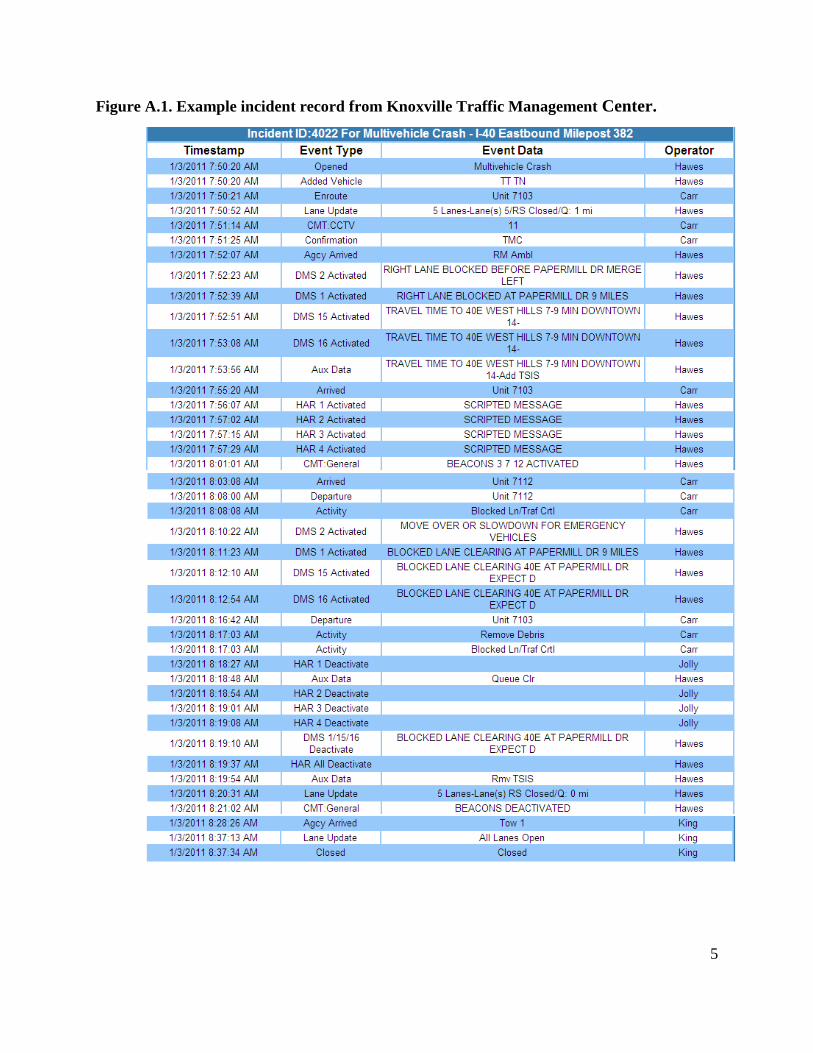
Figure A.1. Example incident record from Knoxville Traffic Management Center.

5

Estimate Reliability Performance

Average travel time and travel time indices were calculated using operations data from the archived data system maintained by TDOT. The calculation procedures to transform field data into travel time–based metrics are the same ones used in SHRP 2 Project L03, Analytical Procedures for Determining the Impacts of Reliability Mitigation Strategies. The first step in this process was to define highway sections over which travel time statistics would be calculated. The data cover all freeways in the Knoxville metropolitan area for a total mileage of 46 miles. The analysis was done separately for each direction of the respective freeways, and thus the directional mileage covered is 92 miles. The following principles were used in defining sections:

• Sections should be relatively homogenous in terms of traffic and geometric conditions. Multiple interchanges are allowed as long as they don’t provide for major drops or additions in traffic volumes along the section.

• Sections should represent portions of trips taken by travelers. Typical distances for urban freeway sections are 3 to 6 miles in length.

• Major bottlenecks, defined as major freeway-to-freeway interchanges, can be present at the downstream end of the section, but never in mid-section.

Eighteen segments were identified in each direction for a total of 36 segments; the average length of each segment was approximately 2.6 miles. The point measurements of volume and speed were converted to travel times over fixed highway distances using a method in widespread use by researchers and practitioners: it is assumed that the point speed measures the travel time over a distance half the distance to the nearest upstream and downstream detectors. This assumption works well if detector spacing is close: ½ mile spacing or less. Figure A.2 shows the process for computing section travel times from individual detectors; this was done at a 5-minute time level.

6

Figure A.2. Converting spot speeds to section travel times.

For each detector zone, vehicle-miles of travel (VMT) and vehicle-hours of travel (VHT) were computed:

VMT = VOLUME * DetectorZoneLength

VHT = VMT/Min(FreeFlowSpeed,Speed)

7

When aggregating to the section level, at least half of the detectors had to report valid data for each of the 5-minute periods; otherwise the data was set to missing. If less than half of the detector data was missing, VMT and VHT were factored up based on the ratio of total section length to the sum of the lengths of the individual detector zones.

For every 5-minute time period in the year, total VMT and VHT were computed. From these, key performance measures were computed:

SpaceMeanSpeed = VMT/VHT

TravelRate = 1/SpaceMeanSpeed

TTI = MAX(1.0,(TravelRate/(1/FreeFlowSpeed)))

Because the bases for the measures are total VMT and VHT, the process is self-weighting. For urban freeways, FreeFlowSpeed is fixed at 60 mph. Note that the TTI was not allowed to be lower than 1.0; thus, speeds higher than 60 mph were set to 60 mph. The reason for this is that the TPO is interested in measuring congestion, not high speeds. If speeds were not capped, the resulting statistics would be biased because of the “credit” given to high speeds. However, the original data was preserved for future examinations.

The congestion metrics were computed for each 5-minute period in a day over the course of a year. For any given analysis time slice (e.g., peak hour, peak period), a TTI distribution and its moments (e.g., 95th percentile TTI) were computed as the VMT-weighted average of all the 5-minute TTIs in that time slice for the entire year. These indices were developed for the a.m. and p.m. peak hours and also for the peak hour shoulders. Table A.1 shows the results for the time period from March 1 to December 31, 2011. These data will serve as the basis for an ongoing annual freeway performance report that the TPO plans to develop. The data will also be used in the modeling portion of the LRTP update.

8

Table A.1. Archived Data Analysis Results

Route Dir Section Peak Period

Average Travel Time

Average Travel Time Index (TTI)

TTI (80th Percentile)




I-140 EB George Williams Road to Kingston Pike AM 1.303 1.002 1.000 1.000 1.008 1.032 I-140 EB George Williams Road to Kingston Pike PM 1.339 1.030 1.000 1.000 1.014 1.664 I-140 WB George Williams Road to Kingston Pike AM 1.456 1.079 1.049 1.222 1.543 2.115 I-140 WB George Williams Road to Kingston Pike PM 1.358 1.006 1.003 1.011 1.027 1.127 I-140 EB Kingston Pike to Dutchtown Road AM 1.693 1.092 1.156 1.253 1.331 1.514 I-140 EB Kingston Pike to Dutchtown Road PM 1.623 1.047 1.043 1.061 1.104 1.480 I-140 WB Kingston Pike to Dutchtown Road AM 1.550 1.069 1.098 1.204 1.307 1.456 I-140 WB Kingston Pike to Dutchtown Road PM 1.509 1.041 1.037 1.050 1.082 1.213 I-275 NB I-40 to Woodland Avenue AM 1.198 1.042 1.037 1.059 1.130 1.383 I-275 NB I-40 to Woodland Avenue PM 1.209 1.051 1.060 1.080 1.138 1.258 I-275 SB I-40 to Woodland Avenue AM 1.210 1.053 1.048 1.066 1.109 1.327 I-275 SB I-40 to Woodland Avenue PM 1.193 1.037 1.045 1.070 1.104 1.210 I-275 NB Woodland Avenue to I-640 AM 1.610 1.039 1.044 1.066 1.112 1.208 I-275 NB Woodland Avenue to I-640 PM 1.654 1.067 1.065 1.110 1.197 1.441 I-275 SB Woodland Avenue to I-640 AM 1.868 1.067 1.074 1.089 1.125 1.207 I-275 SB Woodland Avenue to I-640 PM 1.923 1.099 1.116 1.140 1.169 1.274 I-40 East Section EB I-275 to Cherry Street AM 2.851 1.037 1.049 1.059 1.071 1.110 I-40 East Section EB I-275 to Cherry Street PM 2.939 1.069 1.063 1.098 1.246 1.808 I-40 East Section WB I-275 to Cherry Street AM 2.786 1.032 1.009 1.092 1.237 1.527 I-40 East Section WB I-275 to Cherry Street PM 2.815 1.043 1.003 1.016 1.373 1.869 I-40 East Section EB Cherry Street to I-640 E AM 2.422 1.031 1.042 1.053 1.066 1.128 I-40 East Section EB Cherry Street to I-640 E PM 2.403 1.023 1.016 1.039 1.070 1.269 I-40 East Section WB Cherry Street to I-640 E AM 2.522 1.030 1.033 1.042 1.066 1.156 I-40 East Section WB Cherry Street to I-640 E PM 2.505 1.022 1.027 1.034 1.050 1.150 I-40 East Section EB I-640 E to Asheville Hwy AM 1.978 1.069 1.084 1.103 1.126 1.177 I-40 East Section EB I-640 E to Asheville Hwy PM 1.978 1.069 1.063 1.086 1.142 1.556 I-40 East Section WB I-640 E to Asheville Hwy AM 2.044 1.022 1.028 1.033 1.042 1.090 I-40 East Section WB I-640 E to Asheville Hwy PM 2.055 1.028 1.031 1.038 1.049 1.103

9


Average Travel Time






I-75 NB I-640 to Murray Drive AM 1.699 1.062 1.071 1.077 1.082 1.092 I-75 NB I-640 to Murray Drive PM 1.780 1.112 1.100 1.128 1.188 2.031 I-75 SB I-640 to Murray Drive AM 1.804 1.203 1.224 1.467 1.826 2.781 I-75 SB I-640 to Murray Drive PM 1.590 1.060 1.064 1.080 1.105 1.288 I-640 EB I-40 W to Western Avenue AM 1.003 1.003 1.001 1.005 1.013 1.042 I-640 EB I-40 W to Western Avenue PM 1.020 1.020 1.001 1.011 1.067 1.601 I-640 WB I-40 W to Western Avenue AM 0.642 1.168 1.172 1.374 1.785 2.567 I-640 WB I-40 W to Western Avenue PM 0.559 1.017 1.014 1.041 1.083 1.240 I-640 EB Western Avenue to I-275/I-75 AM 1.480 1.021 1.027 1.041 1.060 1.112 I-640 EB Western Avenue to I-275/I-75 PM 1.658 1.143 1.114 1.439 1.769 2.727 I-640 WB Western Avenue to I-275/I-75 AM 2.074 1.037 1.019 1.055 1.153 1.572 I-640 WB Western Avenue to I-275/I-75 PM 2.021 1.010 1.012 1.016 1.024 1.102 I-640 EB I-275/I-75 to Broadway AM 3.244 1.014 1.016 1.020 1.032 1.068 I-640 EB I-275/I-75 to Broadway PM 3.317 1.037 1.046 1.067 1.113 1.288 I-640 WB I-275/I-75 to Broadway AM 3.135 1.011 1.015 1.020 1.026 1.044 I-640 WB I-275/I-75 to Broadway PM 3.168 1.022 1.023 1.031 1.052 1.145 I-640 EB Broadway to I-40 E AM 3.852 1.027 1.036 1.042 1.052 1.097 I-640 EB Broadway to I-40 E PM 3.832 1.022 1.022 1.032 1.054 1.166 I-640 WB Broadway to I-40 E AM 3.822 1.019 1.024 1.034 1.053 1.073 I-640 WB Broadway to I-40 E PM 3.833 1.022 1.026 1.042 1.070 1.123 I-40 West Section EB Lovell Road to Cedar Bluff Road AM 4.206 1.026 1.027 1.036 1.061 1.151 I-40 West Section EB Lovell Road to Cedar Bluff Road PM 4.453 1.086 1.058 1.191 1.390 2.228 I-40 West Section WB Lovell Road to Cedar Bluff Road AM 4.540 1.020 1.024 1.033 1.056 1.103 I-40 West Section WB Lovell Road to Cedar Bluff Road PM 5.315 1.194 1.335 1.585 1.756 2.373 I-40 West Section EB Cedar Bluff Road to West Hills

(Buckingham Road) AM 2.907 1.020 1.020 1.028 1.043 1.232

I-40 West Section EB Cedar Bluff Road to West Hills (Buckingham Road) PM 3.172 1.113 1.155 1.301 1.495 2.226

I-40 West Section WB Cedar Bluff Road to West Hills (Buckingham Road) AM 2.720 1.046 1.058 1.077 1.104 1.216

10


Average Travel Time






I-40 West Section WB Cedar Bluff Road to West Hills (Buckingham Road) PM 2.790 1.073 1.051 1.097 1.301 2.001

I-40 West Section EB West Hills to I-640 W AM 4.236 1.021 1.019 1.036 1.077 1.216 I-40 West Section EB West Hills to I-640 W PM 4.407 1.062 1.055 1.123 1.242 1.724 I-40 West Section WB West Hills to I-640 W AM 4.257 1.106 1.126 1.148 1.177 1.319 I-40 West Section WB West Hills to I-640 W PM 4.301 1.117 1.127 1.183 1.295 1.868 I-40 West Section WB I-640 W to I-275 AM 4.592 1.044 1.055 1.070 1.092 1.168 I-40 West Section WB I-640 W to I-275 PM 5.532 1.257 1.510 1.681 1.799 2.147 US-129 NB Cherokee Trail to Sutherland Avenue AM 2.608 1.134 1.160 1.217 1.277 1.378 US-129 NB Cherokee Trail to Sutherland Avenue PM 2.633 1.145 1.171 1.193 1.230 1.379 US-129 SB Cherokee Trail to Sutherland Avenue AM 2.285 1.088 1.101 1.126 1.173 1.291 US-129 SB Cherokee Trail to Sutherland Avenue PM 2.351 1.119 1.089 1.147 1.219 3.207

11

Estimate Incident-Related Delay

The incident data were used to estimate incident-related delay. Seven different types of incidents were included in the incident data: single-vehicle crash, multivehicle crash, debris, disabled vehicle, abandoned vehicle, police/ambulance/fire activity, and overturned vehicle. Of these, only three types were considered to cause lane blockage and delay to traffic and were subsequently included in our analysis: single-vehicle crash, multivehicle crash, debris. The other types of incidents typically occur on shoulders of roadways and do not cause lane blockage and traffic delay.

Whereas travel time reliability indices such as the planning time index are based on travel times during normal (incident-free) as well as abnormal (incident-affected) travel conditions, these incident data reflected only abnormal situations. Therefore, it was not possible to calculate any indicators based on the incident data that would be equivalent and comparable to the planning time index. However, to see if the incident data could differentiate between various stretches of freeways from the perspective of incidents and their impact on travel time, the “total duration (in minutes) of incidents per mile” was calculated for each segment of freeway.

The results helped identify a few segments that had relatively high incident duration (i.e., reliability deficiencies). Five segments were identified as problematic locations with a duration that exceeded “the average plus one standard deviation.” Of these, two segments had a duration more than “the average plus two times the standard deviation.” Results for each segment are presented in Table A.2. The sections used are relatively short, which means the sample sizes are probably too low to draw definitive conclusions about the incident performance of the sections. In the future, sections will likely be aggregated to avoid this problem.

Table A.2. Summary Results of Incident Duration per Mile for January–March 2011, for SV Crash, MV Crash, and Debris Combined

Freeway Segment Total Duration of Incidents per Mile

(minutes)

I-40 West Eastbound

1. 374 to 377: Lovell (1/2 mile west) to Cedar Bluff (1/2 mile west) 2. 378 to 380: Cedar Bluff (1/2 mile west) to West Hills (1/2 mile west) 3. 381 to 384: West Hills (1/2 mile west) to I-640 W (1/2 mile west) 4. 385 to 387: I-640 W (1/2mile west) to I-275 (1/2 mile west)

107.50 345.33 * 402.5 ** 139.33

I-40 West Westbound

1. 374 to 377: Lovell (½ mile west) to Cedar Bluff (1/2 mile west) 2. 378 to 380: Cedar Bluff (1/2 mile west) to West Hills (1/2 mile west) 3. 381 to 384: West Hills (1/2 mile west) to I-640 W (1/2 mile west) 4. 385 to 387: I-640 W (1/2mile west) to I-275 (1/2 mile west)

159.9 201.0 139.75 259.33

12

Freeway Segment Total Duration of Incidents per Mile

(minutes)

I-40 East Eastbound 1. 388 to 389: I-275 (1/2 mile west) to Cherry Street (1/2 mile west) 2. 390 to 392: Cherry Street (1/2 mile west) to I-640 E (1/2 mile west) 3. 393 to 394: I-640 E (1/2 mile west) to Asheville Hwy (1/2 mile east)

268 51 217.5

I-40 East Westbound 1. 388 to 389: I-275 (1/2 mile west) to Cherry Street (1/2 mile west) 2. 390 to 392: Cherry Street (1/2 mile west) to I-640 E (1/2 mile west) 3. 393 to 394: I-640 E (1/2 mile west) to Asheville Hwy (1/2 mile east)

240 52 77

I-275 Northbound 1. 0 to 1: I-40 to Woodland Avenue 2. 2 to 3: Woodland Avenue to I-640

303.33 * 255.5

I-275 Southbound 1. 0 to 1: I-40 to Woodland Avenue 2. 2 to 3: Woodland Avenue to I-640

116.67 114.5

I-640 Eastbound

1. 0 to 1: I-40 W to Western Avenue 2. 2 to 3: Western Avenue to I-275/I-75 3. 4 to 6: I-275/I-75 to Broadway 4. 7 to 10: Broadway to I-40 E

116.67 379.5 * 75 23.5

I-640 Westbound

1. 0 to 1: I-40 W to Western Avenue 2. 2 to 3: Western Avenue to I-275/I-75 3. 4 to 6: I-275/I-75 to Broadway 4. 7 to 10: Broadway to I-40 E

494.67 ** 162 129.33 119.5

I-75 Northbound 1. 108 to 110: North of I-640) to Callahan Dr. 115.67 I-75 Southbound 1. 108 to 110: North of I-640) to Callahan Dr. 218.13

I-140 Eastbound

0 & 1: Dutchtown to Kingston Pk 2 & 3: Kingston Pk to Westland 4 & 5: Westland to Northshore 6 to 9: Northshore to TN River

99 59 85 50

I-140 Westbound

0 & 1: Dutchtown to Kingston Pk 2 & 3: Kingston Pk to Westland 4 & 5: Westland to Northshore 6 to 9: Northshore to TN River

151 122 29 16

Average Duration: 163.75 Standard Deviation: 114.66 * Exceeds Average + Standard Deviation (278.41) ** Exceeds Average + 2 x Standard Deviation (393.07)

The analysis of incident duration did not account for the number of lanes that were blocked during each incident, and so it did not reflect the number of vehicles that were delayed. The Knoxville TPO examined detailed incident records for a few selected segments and found that due to the way the data are coded, it would be very time consuming to extract the lane blockage information. There are a few other urban areas where lane blockage information is easily accessible. For example, an analysis of data for Atlanta freeways showed that incidents involving vehicular crashes affect 1.4 times as many lanes as incidents involving debris. So, to incorporate the impact of travel lanes blocked due to an incident, the Knoxville TPO reanalyzed

13

the incident-prone segments of the Knoxville area by weighing the duration due to crashes by 1.5 and the duration due to debris by 1.0. The weighted total duration per mile for these segments did not change the rankings of the segments based on duration.

Table A.3 presents the results of the incident duration/clearance time analysis and shows the average duration of incidents of different types. These results will be used as a baseline in future work by the TPO. For example, the Knoxville TPO wants to include a goal of reducing the duration (clearance time) of incidents on the freeways in its operations plan; the results of the incident duration/clearance time analysis will be used to set a quantifiable objective for this goal. The goal can be accomplished by implementing improved response strategies by TDOT’s incident management operation.

Table A.3. Duration/Clearance Time for Incidents by Type

Type of Incident Average Duration (minutes)

Median Duration (minutes)

Standard Deviation (minutes)

Single-Vehicle Crash 62.95 35 99.15 Multivehicle Crash 49.38 43 35.57 Debris 13.07 7 21.02

A.4 Incorporating Reliability in Policy Statements

Develop Policy Statement

The Knoxville TPO has embraced the concept being promulgated by the Federal Highway Administration of linking transportation operations with transportation planning. The Knoxville TPO is engaged in a variety of activities that may be considered a part of its Planning for Operations program, and the majority of these activities are included in the congestion management process (CMP). The CMP identifies operations projects and strategies, many of which are included in the Metropolitan Transportation Plan.

As a result of this case study, the Knoxville TPO intends to include the improvement of travel time reliability as a specific objective in its CMP. The TPO also intends to craft a reliability target(s) based on a “failure/on-time” reliability performance measure. As an example, the target could be stated this way: “By 2020, reduce the variability in travel time on freeways and major arterials in the region such that 95% of trips along a roadway segment have travel times no more than 1.5 times the average travel time on that segment for a specific time period of the day.” Further work will be required to pick the most relevant performance measure and target numbers.

14

A.5 Incorporating Reliability Measures into Program and Project Investment Decisions

In addition to developing the initial framework for an ongoing performance monitoring system, the case study considered how reliability can be integrated into a current planning process. In Knoxville, the update to the regional ITS architecture was just beginning; the decision was made to explore how reliability can be woven in as well.

Develop a Project List

As part of the Knoxville Regional ITS Architecture Update Study, the Knoxville TPO organized a series of workshops for updating the ITS architecture for the region. These workshops helped identify the market/service packages within each program area that are important for the Knoxville area and establish priorities among these. Market packages represent different types of services that can be provided and projects that can be implemented within each program/service area. One of the products of the ITS architecture update study is a list of specific projects related to respective market/service packages.

The Knoxville TPO decided to estimate the reliability impacts of the operations investments identified in their regional ITS architecture update. Only those projects for which quantified relationships between the investment strategy and the required inputs to the method exist (e.g., segment volume, capacity, free flow speed) were analyzed, as identified in Table A.4. The final project list was developed by consensus of Knoxville ITS architecture and TPO stakeholders.

Table A.4. Knoxville ITS Architecture Projects Analyzed for Benefits

Length 2034 VMT

Region 1 Incident Management Expansion: I-40 and I-75 West of Knoxville Segment 1: I-40 from US-321 (Exit 364) to I-40/I-75 Interchange (Exit 368) 3.53 200,585 Segment 2: I-75 from US-321 (Exit 81) to I-40/I-75 Interchange (Exit 84) 2.68 228,505 Segment 3: I-40/I-75 from I-40/I-75 Interchange (Exit 368) to near Lovell Rd (Exit 374) 6.37 845,083 Region 1 Incident Management Expansion: US-129/SR-115 (Alcoa Hwy) Segment 1: I-140 to Gov. John Sevier Hwy 3.83 230,634 Segment 2: Gov. John Sevier Hwy to near Cherokee Trail 3.39 204,047 Region 1 Incident Management Expansion: I-75 North of Knoxville Segment 1: near Merchant Dr (Exit 108) to Emory Rd (Exit 112) 3.59 313,708 Region 1 Incident Management Expansion: I-140 South of Knoxville Segment 1: near Westland Dr (Exit 3) to US-129 (Exit 11) 8.61 608,238 TDOT Ramp Metering

15

Length 2034 VMT

Segment 1: I-40 from I-140 (Exit 376) to I-640 (Exit 385) 8.23 1,458,962 City of Oak Ridge Traffic Signal System Upgrades Segment 1: Illinois Ave from Robertsville Rd to Tulane Ave 1.04 27,907 Segment 2: Illinois Ave from Tulane Ave to Lafayette Dr 0.89 29,757 Segment 3: Oak Ridge Tpk from Illinois Ave to Florida Ave 2.57 71,577 Segment 4: Lafayette Dr from Oak Ridge Tpk to Bear Creek Rd 1.91 51,590 City of Oak Ridge DMS Deployment Segment 1: Solway to Illinois Ave 3.11 163,840 Cities of Maryville & Alcoa CCTV Camera Deployment Segment 1: US-129 from Pellissippi Pkwy to Hunt Rd 2.19 143,460 Segment 2: US-129 from Hunt Rd to US-411 4.17 212,503 Segment 3: SR-35 from US-129 to US-321 2.66 73,990 City of Knoxville DMS Deployment Segment 1: Kingston Pk from Northshore Dr to Pellissippi Pkwy 9.38 281,355 Combined City of Pigeon Forge & Sevierville Adaptive Signal System Segment 1: SR-66 from I-40 to Chapman Hwy 8.72 362,032 Segment 2: US-441 from Chapman Hwy to Dollywood Ln 7.35 388,252 Segment 3: US-411 (Dolly Parton Pkwy) from SR-66 to Veterans Blvd 1.41 63,467

Select Analysis Method

Because the update to the regional ITS architecture was just beginning, the Knoxville TPO had limited input data consisting of a project list along with segment volumes, capacities, and free flow speeds. The TPO decided to conduct a quick order-of-magnitude assessment of the reliability impacts of projects using the sketch planning methods and the data-poor reliability prediction equations from SHRP 2 Project L03. The objective was to obtain an estimate of total delay (recurring plus nonrecurring) to compare congestion levels with and without the investments in place. This allows them to identify projects offering the highest benefits in terms of reliability.

To support the case study, the SHRP 2 L05 team produced a spreadsheet that operationalizes the data-poor equations from SHRP 2 Project L03. The spreadsheet requires users to input capacity, volume, and length of segment and uses ITS Deployment Analysis System IDAS look-up tables in conjunction with the SHRP 2 L03 data-poor equations to produce several measures of reliability, including the mean TTI, 50th percentile TTI, 80th percentile TTI, and 95th percentile TTI/PTI. It also produces a measure of overall delay that includes nonrecurring delay using the relationship of the economic value of average delay to nonrecurring delay.

16

Estimate Baseline Reliability Benefits

To establish baseline conditions, the team applied a sketch planning approach by using the following steps and equations from the technical reference to estimate reliability without the investment in place:

Compile input data for each analysis segment into a spreadsheet. Input data include directional (D) and peak hour (K) factors, segment length, free flow speed, volume, capacity, and number of lanes, as shown in Table A.5.

Compile average travel time data for each segment into the spreadsheet. For freeway segments, average travel time was calculated using the following equations from NCHRP Report 387 (for uncongested segments) and the work of Ruiter (for congested segments) (Equations 3 and 4 from the technical reference):

𝑡 = 1 + 0.2𝑥10 𝐹𝐹𝑆

for x < 1

𝑡 = 150 ∗ (0.55 + (0.444𝑥−3))

for x ≥ 1

The equations were adapted slightly to calculate average travel time for arterial segments:

𝑡 = 1 + 0.05𝑥10 𝐹𝐹𝑆

for x < 1

𝑡 = 145 ∗ (0.55 + (0.444𝑥−3))

for x ≥ 1

Compute the recurring delay in hours per mile.

RecurringDelay = t – (1/FreeFlowSpeed)

Compute the delay due to incidents (IncidentDelay) in hours per mile. Incident delay can be obtained using basic field data (i.e., segment volumes, capacities, and number of lanes) and the look-up tables from the IDAS User’s Manual.1 This is the baseline incident delay (Du).

1 IDAS User’s Manual, Appendix B, Tables B.2.14–B.2.18, http://idas.camsys.com/documentation.htm.

17

http://idas.camsys.com/documentation.htm

Compute the overall mean travel time index (TTIm) for the baseline condition, which includes the effects of recurring and incident delay:

TTIm = 1 + FFS * (RecurringDelay + IncidentDelay)

The TTIm was used to compute the 80th and 50th percentile travel time indices (TTI80, TTI50) for baseline conditions by using the SHRP 2 L03 data-poor equations:

TTI80 = 1 + 2.1406 * ln(TTIm)

TTI50 = TTIm0.8601

The travel time equivalents (TTIe) for baseline conditions were then calculated by using the following equation:

TTIe = TTIm + a * (TTI80 – TTI50 )

where

TTIe = TTI equivalent on the segment; and

a = reliability ratio (value of reliability/value of time), set equal to 0.8 for now. (Further work is needed to more tightly define the reliability ratio. SHRP 2 Project C04 suggests a range of 0.5 to 1.5, while previous research indicates that the value of reliability varies by trip purpose. A value of 0.8 was used to represent composite trips.)

TTIm was used to compute the planning time index for baseline conditions by using the SHRP 2 L03 data-poor equations:

Planning Time Index = TTI95 = 1 + 3.6700 * ln(TTIm)

Baseline reliability benefits for the regional ITS architecture update projects (as excerpted from the spreadsheet) are summarized in Table A.6.

18

Table A.5. Input Data for Knoxville ITS Architecture Projects

Input Data

Segment Study Period Segment Type Number

of Lanes

Free Flow

Speed

Percent Green Capacity VMT

Peak Hour

Volume 1: I‐40 from US-321 (Exit 364) to I‐40/I-75 Interchange (Exit 368) 1 Freeway 2 65 0 4,145 200,585 3,125 2: I‐75 from US-321 (Exit 81) to I‐40/I-75 Interchange (Exit 84) 1 Freeway 2 65 0 4,145 228,505 4,689 3: I‐40/I-75 from I‐40/I-75 Interchange (Exit 368) to near Lovell Rd (Exit 374) 1 Freeway 2 65 0 6,495 845,083 7,297 1: I‐140 to Gov. John Sevier Hwy 1 Freeway 2 65 0 4,066 230,634 4,215 2: Gov. John Sevier Hwy to near Cherokee Trail 1 Freeway 2 65 0 3,846 204,047 4,213 1: near Merchant Dr (Exit 108) to Emory Rd (Exit 112) 1 Freeway 2 65 0 6,224 313,708 4,806 1: near Westland Dr (Exit 3) to US-129 (Exit 11) 1 Freeway 2 65 0 4,330 608,238 4,945 1: I‐40 from I‐140 (Exit 376) to I‐640 (Exit 385) 1 Freeway 3 65 0 8,299 1,458,962 9,750 1: Illinois Ave from Robertsville Rd to Tulane Ave 1 Arterials(interrupted) 2 45 0.55 2,090 27,907 1,825 2: Illinois Ave from Tulane Ave to Lafayette Dr 1 Arterials(interrupted) 2 45 0.55 2,090 29,757 2,274 3: Oak Ridge Tpk from Illinois Ave to Florida Ave 1 Arterials(interrupted) 2 45 0.55 2,090 71,577 1,894 4: Lafayette Dr from Oak Ridge Tpk to Bear Creek Rd 1 Arterials(interrupted) 2 45 0.55 2,090 51,590 1,837 1: Solway to Illinois Ave 1 Arterials(interrupted) 2 45 0.55 2,090 163,840 3,793 1: US-129 from Pellissippi Pkwy to Hunt Rd 1 Arterials(interrupted) 3 45 0.55 3,135 143,460 4,454 2: US-129 from Hunt Rd to US-411 1 Arterials(interrupted) 2 45 0.55 2,090 212,503 3,465 3: SR-35 from US-129 to US-321 1 Arterials(interrupted) 2 45 0.55 2,090 73,990 1,891 1: Kingston Pk from Northshore Dr to Pellissippi Pkwy 1 Arterials(interrupted) 2 45 0.55 2,090 281,355 2,040 1: SR-66 from I‐40 to Chapman Hwy 1 Arterials(interrupted) 3 45 0.55 3,135 362,032 2,989 2: US-441 from Chapman Hwy to Dollywood Ln 1 Arterials(interrupted) 3 45 0.55 3,135 388,252 3,803 3: US-411 (Dolly Parton Pkwy) from SR-66 to Veterans Blvd 1 Arterials(interrupted) 3 45 0.55 3,135 63,467 3,241

19

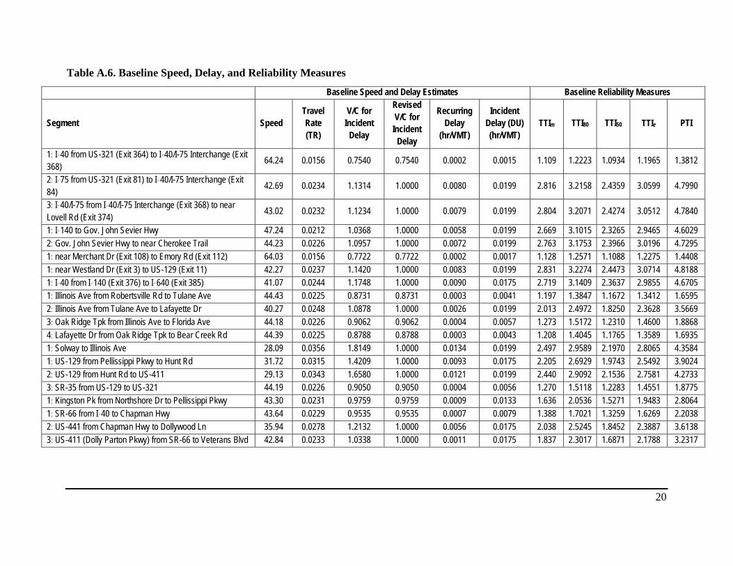
Table A.6. Baseline Speed, Delay, and Reliability Measures

Baseline Speed and Delay Estimates Baseline Reliability Measures

Segment Speed Travel Rate (TR)

V/C for Incident

Delay

Revised V/C for

Incident Delay

Recurring Delay

(hr/VMT)

Incident Delay (DU) (hr/VMT)

TTIm TTI80 TTI50 TTIe PTI

1: I‐40 from US-321 (Exit 364) to I‐40/I-75 Interchange (Exit 368) 64.24 0.0156 0.7540 0.7540 0.0002 0.0015 1.109 1.2223 1.0934 1.1965 1.3812

2: I‐75 from US-321 (Exit 81) to I‐40/I-75 Interchange (Exit 84) 42.69 0.0234 1.1314 1.0000 0.0080 0.0199 2.816 3.2158 2.4359 3.0599 4.7990

3: I‐40/I-75 from I‐40/I-75 Interchange (Exit 368) to near Lovell Rd (Exit 374) 43.02 0.0232 1.1234 1.0000 0.0079 0.0199 2.804 3.2071 2.4274 3.0512 4.7840

1: I‐140 to Gov. John Sevier Hwy 47.24 0.0212 1.0368 1.0000 0.0058 0.0199 2.669 3.1015 2.3265 2.9465 4.6029 2: Gov. John Sevier Hwy to near Cherokee Trail 44.23 0.0226 1.0957 1.0000 0.0072 0.0199 2.763 3.1753 2.3966 3.0196 4.7295 1: near Merchant Dr (Exit 108) to Emory Rd (Exit 112) 64.03 0.0156 0.7722 0.7722 0.0002 0.0017 1.128 1.2571 1.1088 1.2275 1.4408 1: near Westland Dr (Exit 3) to US-129 (Exit 11) 42.27 0.0237 1.1420 1.0000 0.0083 0.0199 2.831 3.2274 2.4473 3.0714 4.8188 1: I‐40 from I‐140 (Exit 376) to I‐640 (Exit 385) 41.07 0.0244 1.1748 1.0000 0.0090 0.0175 2.719 3.1409 2.3637 2.9855 4.6705 1: Illinois Ave from Robertsville Rd to Tulane Ave 44.43 0.0225 0.8731 0.8731 0.0003 0.0041 1.197 1.3847 1.1672 1.3412 1.6595 2: Illinois Ave from Tulane Ave to Lafayette Dr 40.27 0.0248 1.0878 1.0000 0.0026 0.0199 2.013 2.4972 1.8250 2.3628 3.5669 3: Oak Ridge Tpk from Illinois Ave to Florida Ave 44.18 0.0226 0.9062 0.9062 0.0004 0.0057 1.273 1.5172 1.2310 1.4600 1.8868 4: Lafayette Dr from Oak Ridge Tpk to Bear Creek Rd 44.39 0.0225 0.8788 0.8788 0.0003 0.0043 1.208 1.4045 1.1765 1.3589 1.6935 1: Solway to Illinois Ave 28.09 0.0356 1.8149 1.0000 0.0134 0.0199 2.497 2.9589 2.1970 2.8065 4.3584 1: US-129 from Pellissippi Pkwy to Hunt Rd 31.72 0.0315 1.4209 1.0000 0.0093 0.0175 2.205 2.6929 1.9743 2.5492 3.9024 2: US-129 from Hunt Rd to US-411 29.13 0.0343 1.6580 1.0000 0.0121 0.0199 2.440 2.9092 2.1536 2.7581 4.2733 3: SR-35 from US-129 to US-321 44.19 0.0226 0.9050 0.9050 0.0004 0.0056 1.270 1.5118 1.2283 1.4551 1.8775 1: Kingston Pk from Northshore Dr to Pellissippi Pkwy 43.30 0.0231 0.9759 0.9759 0.0009 0.0133 1.636 2.0536 1.5271 1.9483 2.8064 1: SR-66 from I‐40 to Chapman Hwy 43.64 0.0229 0.9535 0.9535 0.0007 0.0079 1.388 1.7021 1.3259 1.6269 2.2038 2: US-441 from Chapman Hwy to Dollywood Ln 35.94 0.0278 1.2132 1.0000 0.0056 0.0175 2.038 2.5245 1.8452 2.3887 3.6138 3: US-411 (Dolly Parton Pkwy) from SR-66 to Veterans Blvd 42.84 0.0233 1.0338 1.0000 0.0011 0.0175 1.837 2.3017 1.6871 2.1788 3.2317

20

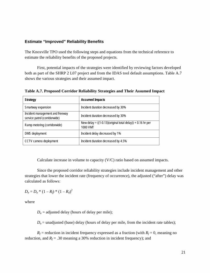
Estimate “Improved” Reliability Benefits

The Knoxville TPO used the following steps and equations from the technical reference to estimate the reliability benefits of the proposed projects.

First, potential impacts of the strategies were identified by reviewing factors developed both as part of the SHRP 2 L07 project and from the IDAS tool default assumptions. Table A.7 shows the various strategies and their assumed impact.

Table A.7. Proposed Corridor Reliability Strategies and Their Assumed Impact

Strategy Assumed Impacts

Smartway expansion Incident duration decreased by 30%

Incident management and freeway service patrol (corridorwide) Incident duration decreased by 30%

Ramp metering (corridorwide) New delay = ((1-0.13)(original total delay)) + 0.16 hr per 1000 VMT

DMS deployment Incident delay decreased by 1%

CCTV camera deployment Incident duration decreased by 4.5%

Calculate increase in volume to capacity (V/C) ratio based on assumed impacts.

Since the proposed corridor reliability strategies include incident management and other strategies that lower the incident rate (frequency of occurrence), the adjusted (“after”) delay was calculated as follows:

Da = Du * (1 – Rf) * (1 – Rd)2

where

Da = adjusted delay (hours of delay per mile);

Du = unadjusted (base) delay (hours of delay per mile, from the incident rate tables);

Rf = reduction in incident frequency expressed as a fraction (with Rf = 0, meaning no reduction, and Rf = .30 meaning a 30% reduction in incident frequency); and

21

Rd = reduction in incident duration expressed as a fraction (with Rd = 0, meaning no reduction, and Rd = .30 meaning a 30% reduction in incident duration).

Changes in incident frequency are most commonly affected by strategies that decrease crash rates. However, crashes are only about 20% of total incidents. Therefore, a 30% reduction in crash rates alone would reduce overall incident rates by 6% (.30 × .20 = .06).

Compute the overall mean travel time index (TTIm) for the improved condition, which includes the effects of recurring and incident delay:


The TTIm was used to compute the 80th and 50th percentile travel time indices (TTI80, TTI50) for improved conditions by using the SHRP 2 L03 data-poor equations:

TTI80 = 1 + 2.1406 * ln(TTIm)

TTI50 = TTIm0.8601

The travel time equivalents (TTIe) for improved conditions were then calculated by using the following equation:

TTIe = TTIm + a * (TTI80 – TTI50)

where

TTIe = TTI equivalent on the segment; and

a = reliability ratio (value of reliability/value of time), set equal to 0.8 for now.

TTIm was used to compute the planning time index for improved conditions by using the SHRP 2 L03 data-poor equations:

Planning Time Index = TTI95 = 1 + 3.6700 * ln(TTIm)

“After” reliability benefits for the regional ITS architecture update projects are summarized in Table A.8.

22

Table A.8. Improved Speed, Delay, and Reliability Measures

Improved Speed and Delay Estimates Improved Reliability Measures

Segment Increased

V/C for Speed

Speed TR Incident

Delay (Da) (hr/VMT)

Recurring Delay

(hr/VMT) TTIm TTI80 TTI50 TTIe PTI

1: I‐40 from US-321 (Exit 364) to I‐40/I-75 Interchange (Exit 368) 0.7540 64.24 0.0156 0.0007 0.0002 1.060 1.124 1.051 1.109 1.213 2: I‐75 from US-321 (Exit 81) to I‐40/I-75 Interchange (Exit 84) 1.1314 42.69 0.0234 0.0097 0.0080 2.156 2.645 1.936 2.503 3.820 3: I‐40/I-75 from I‐40/I-75 Interchange (Exit 368) to near Lovell Rd (Exit 374)

1.1234 43.02 0.0232 0.0097 0.0079 2.145 2.633 1.928 2.492 3.800

1: I‐140 to Gov. John Sevier Hwy 1.0368 47.24 0.0212 0.0097 0.0058 2.010 2.494 1.823 2.360 3.561 2: Gov. John Sevier Hwy to near Cherokee Trail 1.0957 44.23 0.0226 0.0097 0.0072 2.103 2.592 1.896 2.452 3.729 1: near Merchant Dr (Exit 108) to Emory Rd (Exit 112) 0.7722 64.03 0.0156 0.0008 0.0002 1.070 1.145 1.060 1.128 1.249 1: near Westland Dr (Exit 3) to US-129 (Exit 11) 1.1420 42.27 0.0237 0.0097 0.0083 2.171 2.660 1.948 2.517 3.845 1: I‐40 from I‐140 (Exit 376) to I‐640 (Exit 385) 1.0878 44.59 0.0224 0.0175 0.0070 2.594 3.040 2.270 2.886 4.498 1: Illinois Ave from Robertsville Rd to Tulane Ave 0.8084 44.73 0.0224 0.0041 0.0001 1.190 1.372 1.161 1.330 1.638 2: Illinois Ave from Tulane Ave to Lafayette Dr 1.0073 44.30 0.0226 0.0199 0.0004 1.911 2.386 1.745 2.258 3.377 3: Oak Ridge Tpk from Illinois Ave to Florida Ave 0.8390 44.61 0.0224 0.0057 0.0002 1.263 1.500 1.223 1.445 1.858 4: Lafayette Dr from Oak Ridge Tpk to Bear Creek Rd 0.8137 44.72 0.0224 0.0043 0.0001 1.201 1.391 1.170 1.347 1.671 1: Solway to Illinois Ave 1.8149 28.09 0.0356 0.0195 0.0134 2.479 2.943 2.183 2.791 4.332 1: US-129 from Pellissippi Pkwy to Hunt Rd 1.4209 31.72 0.0315 0.0159 0.0093 2.136 2.625 1.921 2.484 3.785 2: US-129 from Hunt Rd to US-411 1.6580 29.13 0.0343 0.0181 0.0121 2.361 2.839 2.094 2.690 4.153 3: SR-35 from US-129 to US-321 0.9050 44.19 0.0226 0.0051 0.0004 1.248 1.474 1.210 1.421 1.813 1: Kingston Pk from Northshore Dr to Pellissippi Pkwy 0.9759 43.30 0.0231 0.0130 0.0009 1.624 2.038 1.517 1.934 2.780 1: SR-66 from I‐40 to Chapman Hwy 0.8513 44.55 0.0224 0.0079 0.0002 1.367 1.669 1.309 1.597 2.148 2: US-441 from Chapman Hwy to Dollywood Ln 1.0832 40.47 0.0247 0.0175 0.0025 1.898 2.372 1.735 2.245 3.352 3: US-411 (Dolly Parton Pkwy) from SR-66 to Veterans Blvd 0.9230 44.01 0.0227 0.0175 0.0005 1.809 2.269 1.665 2.148 3.175

23

Conduct Benefits Analysis

Once the reliability benefits were calculated, the Knoxville TPO conducted a benefits analysis to determine the annual delay savings associated with the candidate projects. Reliability was equilibrated to average travel time through the use of travel time equivalents, so the annual delay savings includes the value of reliability.

For both the baseline and improved condition, the total equivalent delay was calculated based on the TTIe:

TotalEquivalentDelay = (TTIe/FreeFlowSpeed – 1/FreeFlowSpeed) * VMT

where

TotalEquivalentDelay is in vehicle-hours; and

(TTIe/FreeFlowSpeed) = unit travel rate (hours/mile).

The annual delay savings was calculated based on the difference in total equivalent delay between the “before” and “after” scenarios:

AnnualDelaySavings = (TotalEquivDelayBefore – TotalEquivDelayAfter)*260

Prioritize Projects

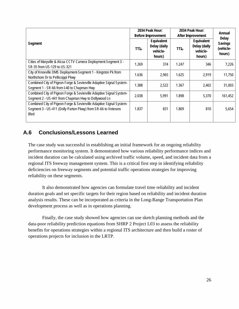
Table A.9 presents the results of applying the benefits methodology. The top five projects offering the highest annual delay savings are as follows:

• Region 1 Smartway Expansion. I-40 and I-75 West of Knoxville, Segment 3: I-40/I-75 from I-40/I-75 Interchange (Exit 368) to near Lovell Rd (Exit 374); 944,973 vehicle-hours of delay savings.

• Region 1 Smartway Expansion. I-140 South of Knoxville, Segment 1: near Westland Dr (Exit 3) to US-129 (Exit 11); 673,920 vehicle-hours of delay savings.

• TDOT Ramp Metering, Segment 1: I-40 from I-140 (Exit 376) to I-640 (Exit 385); 190,091 vehicle-hours of delay savings.

• Region 1 Smartway Expansion. US-129/SR-115 (Alcoa Hwy), Segment 1: I-140 to Gov. John Sevier Hwy; 270,646 vehicle-hours of delay savings.

24

• Region 1 Smartway Expansion. I-40 and I-75 West of Knoxville, Segment 2: I-75 from US-321 (Exit 81) to I-40/I-75 Interchange (Exit 84); 254,505 vehicle-hours of delay savings.

Table A.9. Benefits of Improved Operations, Knoxville TPO ITS Architecture Projects

Segment

2034 Peak Hour: Before Improvement

2034 Peak Hour: After Improvement Annual

Delay Savings (vehicle-hours)

TTIm

Equivalent Delay (daily

vehicle-hours)

TTIm


vehicle-hours)

Region 1 Smartway Expansion - I-40 and I-75 West of Knoxville-Segment 1 - I-40 from US-321 (Exit 364) to I-40/I-75 Interchange (Exit 368)

1.109 303 1.060 169 34,920

Region 1 Smartway Expansion - I-40 and I-75 West of Knoxville-Segment 2 - I-75 from US-321 (Exit 81) to I-40/I-75 Interchange (Exit 84)

2.813 3,621 2.155 2,642 254,505

Region 1 Smartway Expansion - I-40 and I-75 West of Knoxville-Segment 3 - I-40/I-75 from I-40/75 Interchange (Exit 368) to near Lovell Rd (Exit 374)

2.802 13,334 2.144 9,699 944,973

Region 1 Smartway Expansion - US-129/SR-115 (Alcoa Hwy)-Segment 1 - I-140 to Gov. John Sevier Hwy 2.667 3,453 2.009 2,412 270,646

Region 1 Smartway Expansion - US-129/SR-115 (Alcoa Hwy)-Segment 2 - Gov. John Sevier Hwy to near Cherokee Trail 2.761 3,170 2.102 2,280 231,485

Region 1 Smartway Expansion - I-75 North of Knoxville-Segment 1 - near Merchant Dr (Exit 108) to Emory Rd (Exit 112) 1.127 549 1.070 309 62,246

Region 1 Smartway Expansion - I-140 South of Knoxville-Segment 1 - near Westland Dr (Exit 3) to US-129 (Exit 11) 2.829 9,691 2.170 7,099 673,920

TDOT Ramp Metering-Segment 1 - I-40 from I-140 (Exit 376) to I-640 (Exit 385) 2.719 22,282 2.594 21,167 290,091

City of Oak Ridge Traffic Signal System Upgrades-Segment 1 - Illinois Ave from Robertsville Rd to Tulane Ave 1.197 106 1.190 102 892

City of Oak Ridge Traffic Signal System Upgrades-Segment 2 - Illinois Ave from Tulane Ave to Lafayette Dr 2.012 451 1.910 416 9,000

City of Oak Ridge Traffic Signal System Upgrades-Segment 3 - Oak Ridge Tpk from Illinois Ave to Florida Ave 1.273 366 1.263 354 3,142

City of Oak Ridge Traffic Signal System Upgrades-Segment 4 - Lafayette Dr from Oak Ridge Tpk to Bear Creek Rd 1.208 206 1.201 199 1,747

City of Oak Ridge DMS Deployment-Segment 1 - Solway to Illinois Ave 2.496 3,289 2.478 3,261 7,116

Cities of Maryville & Alcoa CCTV Camera Deployment-Segment 1 - US-129 from Pellissippi Pkwy to Hunt Rd 2.205 2,469 2.136 2,365 27,047

Cities of Maryville & Alcoa CCTV Camera Deployment-Segment 2 - US-129 from Hunt Rd to US-411 2.438 4,151 2.360 3,990 41,851

25

Segment

2034 Peak Hour: Before Improvement

2034 Peak Hour: After Improvement Annual

Delay Savings (vehicle-hours)

TTIm


vehicle-hours)

TTIm


vehicle-hours)

Cities of Maryville & Alcoa CCTV Camera Deployment-Segment 3 - SR-35 from US-129 to US-321 1.269 374 1.247 346 7,226

City of Knoxville DMS Deployment-Segment 1 - Kingston Pk from Northshore Dr to Pellissippi Pkwy 1.636 2,965 1.625 2,919 11,750

Combined City of Pigeon Forge & Sevierville Adaptive Signal System-Segment 1 - SR-66 from I-40 to Chapman Hwy 1.388 2,522 1.367 2,402 31,003

Combined City of Pigeon Forge & Sevierville Adaptive Signal System-Segment 2 - US-441 from Chapman Hwy to Dollywood Ln 2.038 5,991 1.898 5,370 161,452

Combined City of Pigeon Forge & Sevierville Adaptive Signal System-Segment 3 - US-411 (Dolly Parton Pkwy) from SR-66 to Veterans Blvd

1.837

831

1.809

810

5,654

A.6 Conclusions/Lessons Learned

The case study was successful in establishing an initial framework for an ongoing reliability performance monitoring system. It demonstrated how various reliability performance indices and incident duration can be calculated using archived traffic volume, speed, and incident data from a regional ITS freeway management system. This is a critical first step in identifying reliability deficiencies on freeway segments and potential traffic operations strategies for improving reliability on these segments.

It also demonstrated how agencies can formulate travel time reliability and incident duration goals and set specific targets for their region based on reliability and incident duration analysis results. These can be incorporated as criteria in the Long-Range Transportation Plan development process as well as in operations planning.

Finally, the case study showed how agencies can use sketch planning methods and the data-poor reliability prediction equations from SHRP 2 Project L03 to assess the reliability benefits for operations strategies within a regional ITS architecture and then build a roster of operations projects for inclusion in the LRTP.

26

B. Florida Department of Transportation (FDOT) B.1 Objective

The objective of this case study is to document the Florida DOT’s efforts to incorporate travel time reliability into its planning and programming process. FDOT has developed reliability measures for both planning (system focused) and operations (corridor focused). These measures are being incorporated into FDOT’s short-range decision support tool, the Strategic Investment Tool (SIT), which is used to prioritize projects for inclusion in the State Transportation Improvement Program (STIP). The Planning Office has also developed modeling techniques for predicting the impact of projects on travel time reliability. In addition, both offices are very interested in the economic value of projects and return on investment of operations improvements.

The case study documents these activities and provides validation for the following steps in the guide:

• Measuring and tracking reliability;

• Incorporating reliability in policy statements; and


B.2 Measuring and Tracking Reliability

Select a Reliability Performance Measure

In 2005, FDOT adopted travel time reliability as a performance measure to be reported to the Florida Transportation Commission on an annual basis. Definitions and data requirements for reporting reliability were developed in 2006, and the FDOT State Traffic Engineering and Operations Office began monitoring travel time reliability on ITS-instrumented corridors in Districts 2, 5, and 7 in 2008. FDOT identified two metrics for travel time reliability: the buffer index (to measure and track the variability of roadway congestion) and the travel time index (to measure and track the congestion level). The travel time and speed data needed to report on reliability are obtained from real-time roadside detectors or vehicle probe data from various sources that report travel time directly. The SHRP 2 L03 project noted that the travel time index is a better measure than the buffer index, so FDOT plans to stop using the buffer index.

27


To enable reporting of reliability at a statewide level, FDOT recognized the need for a predictive model for obtaining the travel time distribution and all associated performance measures for all the freeways in Florida, not just those instrumented with ITS. The Systems Planning Office commissioned the University of Florida to develop a travel time reliability model for the state’s freeway system to address this issue. The model considers various conditions that may occur over a year (e.g., recurring traffic congestion, weather, incidents, and work zones) and calculates the expected travel times for each scenario, along with the expected frequency of occurrence.2 The model assembles the expected travel times and frequency of occurrence to obtain the travel time distribution for a section of roadway, which is then used to calculate reliability-based on-time arrival (percent of time travel speed is greater than 10 mph less than the speed limit) and buffer index (computed as the difference between the 95th percentile travel time and average travel time, divided by the average travel time).

There are differences in travel time between the Operations and Planning Offices due to the different data sources used (i.e., travel time for Operations is based on real-time data, while Planning uses modeled data). FDOT is examining these differences and continuing to refine the travel time reliability model by comparing modeled results to those based on travel time monitoring data.

Regular quarterly meetings are held between Planning and Operations staff to discuss projects and initiatives related to travel time reliability.

Report Reliability Performance

An annual performance report documents FDOT’s short-term objectives, strategies, and progress toward implementing the goals and long-range objectives of the 2060 Florida Transportation Plan.

2 McLeod, D., L. Elefteriadou, and L. Jin. Travel Time Reliability as a Performance Measure: Applying Florida’s Predictive Model on the State’s Freeway System. Presented at 91st Annual Meeting of the Transportation Research Board, Washington, D.C., 2012.

28

B.3 Incorporating Reliability in Policy Statements

Develop Policy Statement

The 2060 Florida Transportation Plan (FTP) defines the state’s long-range goals, objectives, and strategies to guide Florida’s transportation planning and investment decision making over the next 50 years. Travel time reliability is emphasized in the state’s goals to “maintain and operate Florida’s transportation system proactively” and to “improve mobility and connectivity for people and freight.” Reliability is specifically cited in the long-range objectives to “optimize the efficiency of the transportation system for all modes” and “increase the efficiency and reliability of travel for people and freight.”

Performance measures are used to monitor progress toward achieving the 2060 FTP goals and objectives. The plan emphasizes performance monitoring and operations improvements in the following strategies:

• Monitor the physical condition, operational performance, and use of Florida’s transportation system and use these data to inform investment decisions;

• Plan for and deploy a network of sensors and communications infrastructure, along with supporting databases and models, to monitor and manage the performance of critical infrastructure on all modes on a real-time basis; and

• Emphasize transportation systems management and operations strategies to optimize performance of existing facilities.

B.4 Incorporating Reliability Measures into Program and Project Investment Decisions

Develop Funding Scenarios

The Florida Legislature established Florida’s Strategic Intermodal System (SIS) in 2003. It is a statewide network of high-priority transportation facilities and services, including the state’s largest and most significant commercial service airports, spaceport, deepwater seaports, freight rail terminals, passenger rail and intercity bus terminals, rail corridors, waterways, and highways. FDOT is statutorily required to develop and update a plan for implementing the SIS, including a needs assessment, project prioritization process, and finance plan based on anticipated revenue projections, including both 10-year and 20-year cost-feasible components. All designated SIS facilities are eligible for funding from the State Transportation Trust Fund. 29

Funding for the SIS is not modal specific; the programming process gives equal consideration to all components of the SIS, regardless of who owns the facility. At the programming level, performance measures are used to inform the financial policies that determine how funds are allocated across numerous programs such as highway preservation, system expansion, and public transportation.

One of Florida’s biggest challenges has been incorporating reliability (specifically operations improvements) into the programming process. FDOT’s policy is to fund only certain types of projects (i.e., those that expand capacity) with SIS funding. This is a policy decision that was carried over from the Florida Intrastate Highway System that ensures state-managed funds are being used to add capacity to the system. Some types of operations improvements are considered capacity projects and are eligible for funding. For example, FDOT considers managed lanes and auxiliary lanes to be capacity improvements. Intersection/interchange improvements are considered if the project adds lanes or changes the configuration, but traffic signal timing improvements and synchronization are not eligible. Ramp signals are considered if the project involves a redesign of an interchange. Bus rapid transit projects are considered if they include dedicated bus lanes.

At the time of the case study, FDOT was going through its annual programming process and identifying policies or statutory changes that need to be addressed, especially as they affect program funding and target-setting decision making. The FDOT Program and Resource Plan is the best place to make a change in how operations improvements are funded. Policy changes can also occur because of performance data. For example, maintenance conditions are currently exceeding standards in all areas (e.g., maintenance, bridge, and pavement). There is a big difference between current condition and minimum standards, and some of this funding could be directed to other areas such as operations improvements.

Develop a Project List

The SIT is one of the tools used in the project prioritization and select process; it allows FDOT to prioritize projects and investment needs to meet the goals and objectives in the 2060 FTP. The SIT can be used to evaluate highway capacity expansion projects and connector projects currently eligible for SIS funding. Examples are projects that provide additional travel lanes, additional throughput for passenger trips, or operational improvements that provide additional throughput.

The SIT allows users to develop a project list based on scenarios of various proposed project groupings. For example, a district could use the SIT to evaluate all projects in the district currently included in the long-term SIS Unfunded Needs Plan, or a subset of projects for a specific corridor within the district.

30

Detailed information for each project in the SIS Unfunded Needs Plan, Cost Feasible Plan, Work Program, and Multimodal Needs Plan is maintained on the SIT server. This includes project name, facility, roadway ID and begin/end mileposts, project limits, roadway classification, interchange type, bottleneck/grade separation, number of lanes added, and urban/rural classification. Users can also enter detailed project information for projects not currently included in these plans.

Develop Weights for Measures

The SIT allows users to assign a weighting percentage to each of the six goals of the 2060 FTP, as shown in Table B.1. The system defaults to equal weighting of SIS goals, but users can select any weighting combination depending on project type, corridor, or program-level policy objectives. The weighting must always add up to 100%. For example, a user assessing a set of freeway capacity projects might decide that all criteria are equally important and assign weighting percentages equally. An equal weighting for each of the goal areas would be used. A user assessing a set of operations and management projects designed to address nonrecurring delay might assign more weighting to the Maintenance and Operations goal.

Table B.1. Weighting for 2060 FTP Goals

2060 FTP Goal Example Weighting

Safety and security: Provide a safe and secure transportation system for all users 20% Maintenance and operations: Maintain and operate Florida’s transportation system proactively 20%

Mobility and connectivity: Improve mobility and connectivity for people and freight 20% Economic competitiveness: Invest in transportation systems to support a prosperous, globally competitive economy 20%

Livable communities: Make transportation decisions to support and enhance livable communities 10%

Environmental stewardship: Make transportation decisions to promote responsible environmental stewardship 10%

Total weighting 100%

Identify Performance Measures

The SIT evaluates and prioritizes candidate projects based on a set of performance measures that relate to each of the six goals of the 2060 Florida Transportation Plan, as shown in Table B.2. Maximum scores are assigned for each performance measure based on its importance to the goal area, and then a total score is calculated across all performance measures and goal areas.

31

FDOT is in the process of realigning the SIT performance measures to the 2060 Florida Transportation Plan, including adding a measure for travel time reliability. The department has received district comments on the proposed measures and is now in the process of incorporating the measures into the SIT server so they can be used to evaluate projects.

Table B.2. Performance Measures for Strategic Investment Tool

2060 FTP Goal Performance Measures

Safety and security (5 measures)

Crash ratio Fatal crash ratio Bridge appraisal rating Link to military bases Emergency evacuation

Maintenance and operations (4 measures)

Travel time reliability Truck volume (AADTT) Adaptation measure Bridge condition rating

Mobility and connectivity (8 measures)

Connector location Volume to capacity (V/C) ratio Truck percentage (% trucks) Vehicular volume (AADT) System gap Change in V/C or interchange operations Bottleneck/grade separation Delay

Economic competitiveness (14 measures)

Rural areas of critical economic concern Workforce size Educational attainment level Population growth rate Per capita income Freight employment intensity Property taxes Freight transportation infrastructure Military bases employment Per capita income Number of visitors Institutions of higher education Medical centers Tech centers

Livable communities (7 measures)

Residential and community impacts Population density Transit connectivity

32

2060 FTP Goal Performance Measures Bicycle/pedestrian access Managed lanes/special use Social investment/justice Personal safety

Environmental stewardship (14 measures)

Farmlands Geology Archeological/historical sites Contamination Conservation and preservation Wildlife and habitat Flood plains/flood control Coastal/marine Special designations Water quality Wetlands Air quality Energy and sustainability

Estimate the Project Score

Projects are assigned a maximum score for each performance measure based on an established categorization and scoring process described in FDOT’s Strategic Investment Tool Handbook. For travel time reliability, candidate projects are scored a maximum of 8 points based on their expected impact on travel time reliability. Project scores are assigned based on the travel time reliability [i.e., the travel time index (TTI)] for the roadway segment where the project is located.

Roadway segments are assigned an impact category (e.g., high, medium, low) based on the magnitude of their TTI. The facilities with the highest TTI values are considered the worst in terms of reliability (i.e., the facility is unable to consistently handle demand during peak hours and is considered high impact). Projects located on high-impact facilities (i.e., roadways with the worst reliability) are assigned a higher score, while those with lower impact levels score fewer points, as shown in Table B.3.

FDOT is currently in the process of testing the scoring mechanism to see how reliability results affect the ranking of projects. It also plans to incorporate their predictive travel time reliability model into the SIT to provide reliability data at a statewide level. The use of reliability as a performance measure will be part of the decision-making process starting in 2013.

33

Table B.3. Project Scoring for Travel Time Reliability

Travel Time Index Range Impact Category Score

1.261 to 2.04 High 8 1.061 to 1.26 Medium 4 1.00 to 1.06 Low 0

One of the limitations of the SIT is that it is applicable only to evaluating and prioritizing highway capacity expansion projects located on existing roadways. Because the SIT is geometry-based and uses Florida’s current roadway basemap, projects involving new roadway construction or alignments will typically score low because the roadway has not been entered into the basemap. The SIT has never been used to prioritize operations improvements, although it may be possible to use the tool to prioritize these projects as long as those goals are weighted more heavily than the others.

There is currently a gap in performance measures to support economic competiveness, but that goal will be supplemented by a benefit-cost (BC) tool being developed by the Office of Policy Planning. Return on investment (ROI) is currently not included in the SIT because each district and SIS modality has its own methodology for conducting BC analyses and prioritizing projects. The BC tool could provide a way to standardize that process and have common performance measures across all modes. A research and development study to develop the BC methodology was scheduled to be completed by June 2012. Executive management will then decide how to implement the methodology into the SIS programming process going forward.

It is anticipated that the BC tool will be used to calculate ROI for major projects costing more than $50 million. The BC tool will consider forecasted conditions for individual projects (e.g., forecasted traffic volumes, number of lanes) and run an economic analysis to calculate ROI for that project. Operations improvements such as tolled facilities, managed lanes, interchanges, and new facilities would be difficult to incorporate into the methodology from a demand forecast perspective, since it is difficult to forecast traffic volumes for these types of improvements 30 to 40 years out. Tolls are also not intended for program level-analysis. There are thousands of projects on the highway side, and it would be difficult to aggregate ROI results for these projects.

Because the objective of the SIS is to improve through movement, operations improvements could provide significant operational benefits on arterials. Operations improvements could also be implemented as an interim measure to extend the need for capacity improvements. However, FDOT would need the capability to assess how much of an operations budget would contribute to improved reliability. There is a need to instrument more arterials in

34

the future with Bluetooth or other technology to collect real-time speed data to support this level of analysis.

B.5 Conclusions/Lessons Learned

The Florida DOT case study revealed that incorporating reliability (specifically operations projects) into the programming process is a challenging process for most state DOTs. It requires locating a specific funding category to cover operations improvements, although statutory requirements may limit the types of projects that can be funded with existing funding categories. The extent to which this will change as a result of Moving Ahead for Progress in the 21st Century (MAP-21) is still to be determined. Two basic funding models can be considered: (1) allocating separate funding for operations projects, or (2) allocating a portion of existing capacity funding for operations projects. This has important implications for the SHRP 2 L05 project, as it appears many states would benefit from guidance on determining eligibility of funding operations improvements under specific silos or funding categories or making the required policy changes to set up a dedicated funding mechanism. However, because different state DOTs have different programming priorities and processes, it may be difficult to identify a good decision-making model for the long term.

The case study validated the following success factors for incorporating reliability into the planning and programming process:

• Reliability needs to be specifically addressed in the vision, mission, and goals of a plan. These policy statements define the long-term direction of an agency and provide the foundation on which to select reliability performance measures and make the right choices and trade-offs when setting funding levels and selecting projects.

• Reliability needs to be a well-defined measure with supporting data. Well-defined reliability performance measures define an important, but often overlooked, aspect of customer needs. The measures help support the development of policy language and are critical to making reasoned choices and balanced trade-offs.

• Reliability needs to be used to estimate/predict transportation needs and deficiencies including the development and analysis of project/scenario alternatives. Estimating reliability deficiencies by using well-defined measures helps define the size and source of the reliability problem; this information can be used to inform policy makers about how the reliability of the system has been changing over time and how it is expected to change in the future. The maps, charts, and figures provide critical background when making choices and trade-offs.

35

• Reliability needs to be used in program-level trade-offs. Bringing reliability into the discussion brings clarity to the issue of balancing operations and capacity funding. Without the consideration of reliability, the trade-off nearly always tilts toward capacity projects.

• Reliability needs to be an integral component of priority setting/decision making at the project level. Incorporating reliability into project prioritization and programming brings clarity to the issue of choosing the appropriate balance of operations and capacity strategies.

State DOTs would benefit from a maturity model that defines various levels of organizational capability with respect to these success factors. State DOTs could use the maturity model as a tool for (1) assessing where they stand with respect to incorporating reliability into all components of the planning and programming process, (2) helping them understand common concepts related to the process, and (3) helping them identify next steps to achieve an ultimate goal state. The maturity model should be a living document that is continually refined based on agency capabilities.

36

C. Los Angeles Metropolitan Transit Authority C.1 Objective

The objective of the Los Angeles (LA) County Arterial Performance Monitoring case study is to develop the preliminary framework for an arterial performance monitoring system, which is being developed by the Los Angeles Metropolitan Transit Authority (LAMTA) as an improved mechanism for prioritizing arterial operations projects for funding.

This case study documents these activities and provides validation for the “measuring and tracking reliability” step in the guide.

C.2 Background

As part of its 2009 Long-Range Transportation Plan (LRTP), LAMTA continues to focus on improving arterial traffic flow through the implementation of transportation system management (TSM) projects, including intelligent transportation systems (ITS), coordinated signal timing, and bus signal priority. Historically, LAMTA has programmed over $30 million per year to meet regional and subregional needs for projects of this nature. Due to a number of financial constraints, the 2009 LRTP strategic plan calls for a 50% reduction in TSM funding over the next 30 years. LAMTA has annual solicitations for agencies in LA County to apply for funding to improve arterial operations.

LAMTA’s current process for prioritizing arterial operations projects involves conducting before and after evaluations. Data is collected using floating car surveys and spot counts. It is a reactive approach in response to incidents and complaints received from the traveling public. The approach is based on local-level evaluation using optimization.

Due to the limited amount of funding that will be available for future TSM projects, LAMTA is looking for an improved way to prioritize projects that will also set the groundwork for using performance monitoring to improve day-to-day operations. This will be accomplished through the development of an arterial performance and reliability measurement system that will

• Feed into the prioritization of program needs;

• Aid in the continuous reevaluation of the mobility and reliability benefits of completed projects; and

• Include the proper balance between private vehicle and transit priority.

Information generated from the system will be used to

37

• Guide future planning investment decisions;

• Aid in project development activities;

• Provide insight into the development of a more quantitative approach to project and programming prioritization;

• Assess the impact of TSM improvements on bus operations; and

• Provide a tool for improved management of the transportation system.

C.3 Measuring and Tracking Reliability

Select a Reliability Measure

LAMTA and its subregional partners determined that they need an improved way to prioritize projects that incorporates multimodal reliability. They developed a list of key arterial performance and reliability measures needed to quantify the mobility benefits of individual TSM projects and to demonstrate the efficacy of the overall TSM program. The primary measures of effectiveness (MOEs) that will measure their objectives are travel time and travel time reliability. Surrogate measures of travel time or travel time reliability were also considered. These include

• Level of service,

• Volume,

• Occupancy,

• Speed,

• Travel times,

• Vehicle delay,

• Greenhouse gas emissions, and

• Fuel reduction.

38

Assess Data Sources

LAMTA assembled existing sources of available arterial data in the region that can be used to derive the arterial performance and reliability measures. There were two sources of data: detector data from signal systems and transit automatic vehicle location (AVL) data. LAMTA reviewed each of these data sources with respect to their ability to support to the desired metric, including data availability, data quality, and costs to collect/analyze the data; they determined that data to drive these measures is an issue, in terms of both coverage and consistency across jurisdictions.

For detector data, LAMTA determined that existing detectors have gaps geographically, may not be presented or stored in a consistent manner, and may not be able to derive travel time well. LAMTA has a large archive of transit AVL data, so this was examined as another potential data source. The systems in use in LA County also track dwell time. LAMTA verified that travel time and speeds from door opening to door opening are available and could be used to measure bus travel time. LAMTA will continue to investigate how well that data might be able to meet its needs.

LAMTA also investigated types of surrogate measures that could be calculated with transit data. One approach is to calibrate bus travel time with passenger vehicle travel time and utilize a factor that calculates passenger vehicle travel time. One concern over using the bus travel tame data is that the relationship between bus travel times and passenger vehicle travel times will likely vary depending on level of congestion and speed of traffic. The calibration may need to be undertaken over a broad range of speeds to be accurate. Another concern is that there are a limited number of data points because there are limited numbers of coaches that travel any given arterial. Finally, there are some arterials on which LAMTA would like to measure performance that have no transit service or such infrequent transit service that performance cannot be measured. Getting robust reliability results from this type of data could be challenging.

Based on this assessment, LAMTA staff defined data gaps and alternative data sources that could be used to support the desired arterial performance and reliability measures, such as advanced detection and probe vehicles. LAMTA investigated third-party data sources from the private sector and received a sample set of data for arterials. The staff also assembled high-level cost information for those data. The data include many observations and can provide robust reliability information. However, it is possible that LAMTA will want to measure performance on roadways that do not have sufficient probes to accurately measure reliability. Also, LAMTA is concerned about the long-term cost for the data.

LAMTA also evaluated existing arterial performance measurement systems in coordination with other project initiatives under way throughout LA County. This included proposing alternative approaches to partners for consensus development, identifying a strategy to

39

fill gaps (including deployment of additional detection systems, if needed), and proposing funding for data development and a demonstration system.


LAMTA is analyzing a number of approaches for calculating performance measures based on available data sources. These include the following options:

• Using existing data sources, primarily the data from arterial signal systems;

• Using transit AVL data;

• Using third-party arterial data; and

• Using a hybrid option that includes portions of each.

LAMTA developed a high-level approach to performance measurement to support its arterial operations program based on these options. The next step will be the development of a proposed strategy for an arterial performance management system and its components.

C.4 Conclusions/Lessons Learned

This case study documented the development of a preliminary framework for an arterial performance monitoring system. The case study results show that arterial reliability measures require robust data sets that provide sufficient data points on each roadway of interest during all times of interest. Although it is possible to calculate arterial reliability measures from a variety of multimodal data sources, there is a challenge in collecting large enough samples both spatially and temporally. Data source consistency is critical.

40

D. Southeast Michigan Council of Governments D.1 Objective

The Southeast Michigan Council of Governments (SEMCOG) is the metropolitan planning organization (MPO) for the Detroit region. As in many regions, the identified need for infrastructure improvements greatly outweighs the available funding levels, so a logical and effective process is needed to assist SEMCOG in setting program funding levels. The council developed such a process while preparing its 2035 Regional Transportation Plan (RTP). That plan allows trade-offs among several program areas, including pavement, bridge, highway capacity, safety, transit, and nonmotorized modes. This case study updates that process to assess funding levels required for SEMCOG’s roadway operations program by assessing total delay, including nonrecurring delay, the main cause of unreliable travel.

The case study provides validation for the “incorporating reliability into program and project investment decisions” step in the guide.

D.2 Background

As part of its planning process, SEMCOG has developed a new approach for setting program-level funding. Setting program-level funding (1) helps build consensus on the region’s transportation priorities and helps ensure that the projects included in the RTP support these priorities, (2) provides decision makers with the quantitative information they need to fully understand the consequences of their investment choices, and (3) enables SEMCOG to develop an RTP that is realistic in terms of how much it will cost and how much it can achieve.

To set program funding levels, SEMCOG follows these steps:

1. Define measures of effectiveness and assess current performance.

2. Analyze the relationship between funding and performance within each program area.

3. Develop funding scenarios (each scenario represents a different way of splitting anticipated funds across the program areas used in the RTP).

4. Present the results of the analysis to decision makers in a format that enables them to conduct program-level trade-offs, with the goal of reaching consensus on long-range funding and performance targets for the region.

Since the completion of the 2035 RTP, SEMCOG has developed a performance curve for the roadway operations program by using recurring delay as the MOE. Figure D.1 shows the

41

performance curve for the roadway operations program using recurring delay. This case study updates the MOE to total delay, which includes recurring and nonrecurring delay.

Figure D.1. SEMCOG roadway operations investment levels mapped to average recurring delay.

This case study reviewed the measure currently used for highway capacity and identified a potential system measure more appropriate for assessing highway operations. An analysis methodology for prioritizing operations strategies and capital improvements using reliability was also developed and tested as part of the case study.

D.3 Incorporating Reliability into Program and Project Investment Decisions

Define Measures of Effectiveness

Measures of effectiveness (MOEs) are measures that indicate how a system is performing. Essentially, an MOE is a single, exemplar performance measure used to indicate the performance of an entire program area. While agencies typically use performance measures to indicate the many different aspects of performance (that is, for safety, an agency might consider total fatalities, pedestrian and bicycle crashes, serious injury crashes, and rates of the same), they use

0.0

0.5

1.0

1.5

2.0

2.5

0 25 50 75 100 125 150

Hou

rs o

f Del

ay p

er 1

,000

VM

T

Annual Budget ($ million)

Analysis of Operations Investment Levels

42

MOEs as a sort of best-fit performance measure or a measure that represents the gist of what makes a program area important. To that end, SEMCOG selected MOEs for each of its program areas (see Table D.1). SEMCOG incorporated reliability into the MOE for the Roadway Operations program area by estimating nonrecurring hours of congestion delay in addition to typical recurring hours of congestion delay. Defining the MOE in this way allowed SEMCOG to retain consistency with the Highway Capacity program area MOE which measures hours of recurring congestion delay.

Table D.1. Measures of Effectiveness Used in Prioritization Process

Program Area MOE

Pavement preservation Percent of pavement in good or fair condition Highway capacity Hours of (recurring) congestion delay per 1,000 vehicle miles

traveled Bridge preservation Percent of bridges in good or fair condition Safety Fatalities per 100 million vehicle miles traveled Transit Extent of the transit network (the existing network or the region’s

transit vision) Nonmotorized Percent of population and employment within ½ mile of a

nonmotorized facility Roadway operations Hours of (recurring and nonrecurring) congestion delay per 1,000

vehicle miles traveled

Define Representative Corridors

SEMCOG had limited resources and time to invest in the analysis. Understanding this, they estimated the roadway operations MOE by selecting several representative freeway corridors within the region and expanding the results of these analyses to represent a regionwide MOE. These corridors each have operational characteristics—such as average traffic volume, interchange density, directional flows, and surrounding land use—that are representative of many other corridors throughout the Detroit region. The representative corridors all are freeway/limited-access roadways and include an urban radial (Interstate 96), a suburban radial (Interstate 75), and a suburban beltway (Interstate 275). SEMCOG estimated the operations MOE on these representative corridors and expanded the results to the entire region.

Data were collected for the representative corridors, including baseline peak period volumes, capacities, number of lanes, VMT, and speeds (congested and posted). All of these data were obtained from the validated regional travel demand model. The representative urban radial corridor has four lanes, a capacity of 24,000 vehicles per hour, and a volume of 18,200 vehicles per hour; the suburban radial has two lanes, a capacity of 12,000 vehicles per hour, and a volume 43

of 8,900 vehicles per hour; and the suburban beltway has three lanes, a capacity of 18,000 vehicles per hour, and a volume of 15,875 vehicles per hour. Table D.2 lists the details of each representative corridor.

Table D.2. Representative Corridor Details

Representative Corridor Lanes Capacity

(Vehicles per Hour)

Volume per Hour

Urban Radial (I-96) 4 24,000 18,200

Suburban Radial (I-75) 2 12,000 8,900

Suburban Beltway (I-275) 3 18,000 15,875

Use Representative Corridors to Represent Regionwide Analysis

SEMCOG developed a regionwide analysis by identifying the percentage of regional VMT that each corridor accounts for. Based on professional judgment and historical traffic data, SEMCOG determined that urban radials carry 37% of regional VMT, suburban radials carry 30% of regional VMT, and suburban beltways carry 33% of regional VMT. Because it opted to use a rate-based MOE, SEMCOG was able to use the delay rate from the representative corridors as a proxy for delay on all other similar corridors in the region. Finally, the representative corridors were rolled up into a regionwide value by taking a VMT-weighted average of total delay. Table D.3 shows the percentage of regional VMT by representative corridor and provides an example calculation of the weighted average of total delay given an illustrative delay of 5, 4, and 3 hours of total delay per 1,000 VMT for the urban radial, suburban radial, and suburban beltway corridors, respectively. While this method can be used to estimate the change in the rate of delay in the region under different funding scenarios for major corridors, it cannot be used to estimate total delay in the region, as travel on many additional minor corridors and arterials is not represented by the selected analysis corridors.

Table D.3. Representative Corridor Vehicle Miles Traveled

Representative Corridor Percentage of Regional Vehicle Miles Traveled

(VMT)

Example MOE Result–Total Delay (hours/1,000 VMT)

Urban Radials 37 5

Suburban Radials 30 4

44

Develop Funding Scenarios

The analysis team applied professional judgment to simplify the regional analysis. Instead of a more rigorous approach requiring development of lists of specific projects and individual analysis of their cost, SEMCOG used experience with previous deployments of these types of strategies to make a high-level estimation of how much operations-type investment could be built given different funding levels. For example, $50 million in funding would allow them to invest in a roadway operations program covering 75% of the VMT on urban radials, 50% of the VMT on suburban radials, and 50% of the VMT on suburban beltways. Note that as part of this process, SEMCOG prioritized funding on urban radial corridors while funding suburban radials and suburban beltways at similar rates. Table D.4 shows the coverage of roadway operations projects on regional facilities under the different investment levels.

Table D.4. Regional Coverage of Roadway Operations Assumed for Various Investment Levels

Investment Level

Representative Corridor $25M $50M $75M $100M

Urban Radial 50% 75% 100% 100%

Suburban Radial 25% 50% 75% 100%

Suburban Beltway 25% 50% 75% 100%


SEMCOG considered several optional approaches for conducting the relability analysis:

• Development of a sketch planning methodology using SHRP 2 L03 data-poor equations; or

• Incorporation of postprocessing methods with the existing travel demand model, such as the pairing of the travel demand model with the FHWA’s ITS Deployment Analysis System (IDAS) software.

Suburban Beltways 33 3

Regionwide 100 4.04 = 5 X 0.37 + 4 X 0.30 + 3 X 0.33

45

Weighing the analysis resources (time, money, and staff), the ease of the analysis method and the ready availability of data to support the analysis, and the need for high-level assessment of the investment levels, SEMCOG identified the sketch planning approach based on SHRP 2 L03 methods as the preferred approach.

Collect Data

Data for this analysis included baseline peak period volumes, capacities, number of lanes, VMT, and speeds (congested and posted). These data were obtained from SEMCOG’s validated regional travel demand model on a link-by-link basis and summed/averaged across the representative corridors. Free flow and congested travel times were estimated by dividing the link lengths by the compiled travel speeds.

Estimate Baseline Delay on Representative Corridors

To support the case study, the SHRP 2 L05 team produced a spreadsheet that operationalizes the data-poor equations from SHRP 2 Project L03. The spreadsheet requires users to input capacity, volume, and length of segment and uses IDAS look-up tables in conjunction with the SHRP 2 L03 data-poor equations to produce several measures of reliability, including the mean TTI, 50th percentile TTI, 80th percentile TTI, and 95th percentile TTI/PTI. It also produces a measure of overall delay that includes nonrecurring delay using the relationship of the economic value of average delay to nonrecurring delay.

For this analysis, the peak period was defined as the peak 3 hours during the morning commute (6 a.m. to 9 a.m.), consistent with the data available in the regional travel demand model. Recurring delay was estimated by subtracting free flow travel times from congested travel times using Equation 7 from the technical reference:

RecurringDelay = t – (1/FFS)

Then incident-related delay was estimated using FHWA’s IDAS look-up tables based on number of lanes, length of the peak period, and volume to capacity ratio. Table D.5 shows an excerpt of the larger table, specific to the urban radial corridor. The incident-related delay factors represent the expected amount of incident delay that would be incurred at different levels of congestion (as measured by the V/C ratio) and the number of roadway lanes. The selected factor was applied on a link-by-link basis to the VMT on the facility to estimate the expected incident-related delay.

46

Table D.5. IDAS Incident-Related Delay Factors for 3-Hour Peak Period

Volume/1-Hour Level-of-Service Capacity

Number of Lanes 2 3 4+

0.15 3.71E-08 1.62E-09 5.45E-12 0.3 5.66E-07 5.21E-08 7.22E-10 0.45 2.79E-06 3.97E-07 1.26E-08 0.6 8.63E-06 1.68E-06 9.57E-08 0.75 2.07E-05 5.14E-06 4.61E-07 0.9 4.25E-05 1.28E-05 1.67E-06 1.05 7.78E-05 2.77E-05 4.95E-06 1.2 0.000132 5.41E-05 1.27E-05 1.35 0.000209 9.77E-05 2.91E-05 1.5 0.000316 0.000166 6.12E-05 1.65 0.00046 0.000267 0.00012 1.8 0.00065 0.000413 0.000221 1.95 0.000901 0.00062 0.000389 2.1 0.001245 0.000912 0.000656 2.25 0.00177 0.00135 0.001074 2.4 0.002722 0.002115 0.001742 2.55 0.004772 0.003798 0.003011 2.7 0.009674 0.00828 0.006586 2.85 0.014859 0.012966 0.010231 3 0.01986 0.01744 0.01368

Source: IDAS User’s Manual, 2004.

Incident-related delay, however, does not account for the total nonrecurring delay. To estimate the total delay, the algorithms for travel time equivalents (Equation 21) and total equivalent delay (Equation 22) from the SHRP2 L03 study were used. They provide estimation techniques for situations in which limited data are available regarding these additional causes of nonrecurring congestion. Total equivalent delay for the region was then estimated by extrapolating the total delay by VMT factors to estimates of the regional VMT by representative corridor type. This resulted in an overall regional MOE of 6.8 hours of total delay per 1,000 VMT. Thus, including reliability in this assessment increased the estimate of delay to more than double the measure when only recurring travel time was considered (see Table D.6).

47

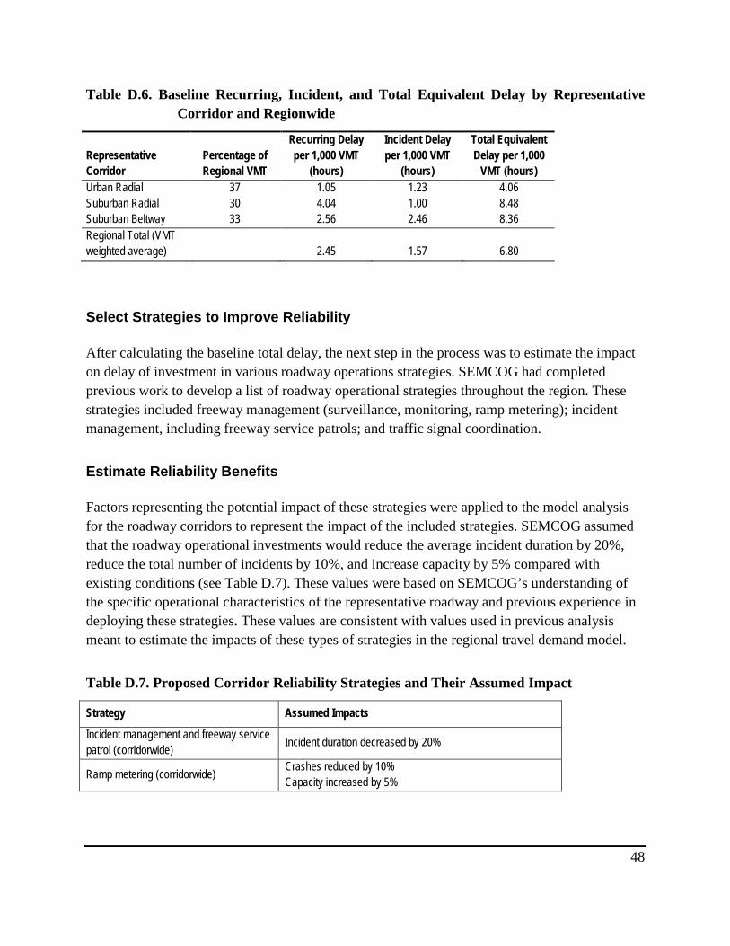
Table D.6. Baseline Recurring, Incident, and Total Equivalent Delay by Representative Corridor and Regionwide

Representative Corridor

Percentage of Regional VMT

Recurring Delay per 1,000 VMT

(hours)

Incident Delay per 1,000 VMT

(hours)

Total Equivalent Delay per 1,000

VMT (hours) Urban Radial 37 1.05 1.23 4.06 Suburban Radial 30 4.04 1.00 8.48 Suburban Beltway 33 2.56 2.46 8.36 Regional Total (VMT weighted average) 2.45 1.57 6.80

Select Strategies to Improve Reliability

After calculating the baseline total delay, the next step in the process was to estimate the impact on delay of investment in various roadway operations strategies. SEMCOG had completed previous work to develop a list of roadway operational strategies throughout the region. These strategies included freeway management (surveillance, monitoring, ramp metering); incident management, including freeway service patrols; and traffic signal coordination.

Estimate Reliability Benefits

Factors representing the potential impact of these strategies were applied to the model analysis for the roadway corridors to represent the impact of the included strategies. SEMCOG assumed that the roadway operational investments would reduce the average incident duration by 20%, reduce the total number of incidents by 10%, and increase capacity by 5% compared with existing conditions (see Table D.7). These values were based on SEMCOG’s understanding of the specific operational characteristics of the representative roadway and previous experience in deploying these strategies. These values are consistent with values used in previous analysis meant to estimate the impacts of these types of strategies in the regional travel demand model.

Table D.7. Proposed Corridor Reliability Strategies and Their Assumed Impact



Ramp metering (corridorwide) Crashes reduced by 10% Capacity increased by 5%

48

SEMCOG used Equation 9 from the technical reference to estimate the impact of these programs on nonrecurring congestion.

Da = Du * (1 – Rf) * (1 – Rd)2

where

Da = adjusted delay (hours of delay per mile);

Du = unadjusted (base) incident delay from the IDAS incident delay look-up tables (hours of delay per mile);

Rf = reduction in incident frequency expressed as a fraction (with Rf = 0, meaning no reduction, and Rf = .30, meaning a 30% reduction in incident frequency); and

Rd = reduction in incident duration expressed as a fraction (with Rd = 0, meaning no reduction, and Rd = .30, meaning a 30% reduction in incident duration).

The incremental benefits for the representative corridors were extrapolated to the regional level by estimating the proportion of the regional network comprising the representative corridors and applying the incremental benefits to regionwide estimates of total travel time, similar to the estimation of the baseline measure.

Develop Performance Curve

SEMCOG subtracted the savings from roadway operations improvements under different annual budgets from the baseline total delay (5.58 hours of total delay per 1,000 VMT) to show how different funding levels affect the MOE. Table D.8 shows how different levels of investment affect total delay.

Table D.8. Benefits of Roadway Operations Investments

Representative Corridor

Percentage of Regional VMT

Savings in Total Delay per 1,000 VMT (hours) $0M $25M $50M $75M $100M

Urban Radial 37 4.06 3.06 2.56 2.05 2.05 Suburban Radial 30 8.48 7.12 5.77 4.41 3.06 Suburban Beltway 33 8.36 7.62 6.87 6.12 5.37 Regional Total (VMT weighted average)

6.80 5.78 4.94 4.10 3.45

49

The result of this analysis was an improved performance curve, better representing trade-offs in investment levels in reliability mitigation strategies mapped to regional benefits in total travel time delay (including recurring and nonrecurring travel time benefits). Figure D.2 shows the benefits of roadway operations investments (Table D.8) graphically.

Figure D.2. Investment curve.

As SEMCOG invests more in roadway operations, total delay is reduced. The comparison of benefits estimated both with and without considering reliability show that investments in the operations strategies yield a much greater impact on total hours of delay, particularly at the lower investment levels. Small investments in these strategies result in a steep curve of reducing delay levels. Similar to the curve not considering reliability, there is a declining utility to higher investment levels; increased investment brings about lower incremental improvement for each dollar spent.

SEMCOG now can balance program-level funding among pavement preservation, highway capacity, bridge preservation, safety, transit, nonmotorized, and roadway operations.

D.4 Conclusions/Lessons Learned

The comparison of the benefits estimated both with and without considering reliability shows several interesting results. Key findings include the following:

0.00

1.00

2.00

3.00

4.00

5.00

6.00

7.00

8.00

$0 $20 $40 $60 $80 $100

Equi

vale

nt D

elay

(Hou

rs/1

,000

VM

T)

Annual Budget (Millions)

50

• As expected, when nonrecurring delay is considered in the analysis, the overall delay estimates are much greater (with the baseline delay more than doubling from 2.4 to 6.8 hours of delay per 1,000 VMT).

• Investments in roadway operations strategies were shown to a yield a much greater impact on total hours of delay, particularly at the lower investment levels. Small investments in these strategies result in a steep curve of reducing delay levels.

• Similar to the analysis, which does not considering reliability, there is a declining utility to higher investment levels; increased investment brings about lower incremental improvement for each dollar spent.

In addition to the actual analysis results, several lessons were learned throughout the case study:

• Reliability can be relatively easily incorporated in the trade-off analysis process. Consideration of reliability will likely have an impact on the results of the prioritization process.

• The use of representative corridors can be effective in conducting a regional analysis within reasonable budget and schedule requirements.

• Even in situations with limited data availability, assessments of reliability can be performed efficiently, providing much needed consideration of these factors within the overall assessment of trade-offs regarding investment priorities.

The analysis approach represented in this case study represents a first step in the overall incorporation of reliability performance measures in the investment prioritization process. Improvements and enhancements to this process may include the following:

• Application of nonrecurring congestion measurement within the analysis of highway capacity improvements to make the comparison of capacity and operations improvements more equitable (e.g., capture the reliability benefits of increasing capacity).

• Inclusion of a greater variety of representative corridors in the analysis.

• Development of automated routines to allow the estimation of incident related delay and total delay (recurring and nonrecurring) within the travel demand model itself, thus allowing more detailed regional assessment of these measures.

51

• Separating the various roadway operations improvements within the analysis to allow each strategy to be analyzed individually.

52

E. Colorado DOT/Denver Regional Council of Governments E.1 Objective

This case study establishes baseline conditions for a pilot corridor and lays the groundwork for conducting a before/after analysis to assess benefits of operations strategies using an arterial performance monitoring system. It documents the steps to plan and fund an operations project intended to improve travel time reliability. Finally, the case study documents the Colorado DOT’s (CDOT) efforts in selecting and incorporating operations (including reliability) performance measures into their long-range planning process.

This case study provides validation for the following steps in the guide:

• Measuring and tracking reliability; and


E.2 Background/Purpose

The Denver Regional Council of Governments (DRCOG), in partnership with the City of Englewood and Colorado DOT, recognized the need to start collecting mobility and travel time data on the arterial network to support the long-range planning process. In a pilot effort, an inexpensive arterial performance monitoring system was implemented along a segment of Hampden Avenue, a major arterial in Denver. The Hampden Avenue project is approximately 7 miles long and includes 11 signalized intersections. The system consists of Bluetooth travel time detectors, queue length detectors, and volume counters installed at various locations throughout the corridor to monitor travel time and planning time indices. The system will be operational in spring 2013. The purpose of the pilot project is to provide operators with information that will help them better manage their arterial roadways, and to provide travelers with better traveler information which will result in improved travel time reliability. Continuous monitoring of corridor performance will provide CDOT and decision makers with quantifiable information on the reliability impacts of specific operations improvements that are implemented along the corridor, as well as an estimate of the total impact of all improvements made to the corridor or network.

The project partners plan to use the monitoring results to develop a portfolio of operations strategies that will be evaluated, selected, designed, and implemented within a performance-based system. Potential operations strategies could include traffic management (e.g., signal retiming, ITS deployment, intersection improvements, geometric improvements, and roundabouts), incident management, pavement maintenance, bridge maintenance, transit, nonmotorized facilities, freight/goods movement, winter operations, and capacity expansion 53

projects. The system will demonstrate to decision makers, taxpayers, and users that projects were selected to meet specific performance goals, were implemented as high-priority projects based on performance criteria, and provide specific user benefits in terms of improving corridor and system reliability. Incremental improvement in benefits over time will allow the partner agencies to shift resources to operations investments.

E.3 Measuring and Tracking Reliability

The first part of the case study demonstrates the methodology for analyzing travel time data and calculating various reliability performance indices based on traffic flow data collected using the pilot arterial performance monitoring system. The results will be used to establish baseline conditions for the Hampden Avenue corridor, which is a critical first step in conducting a before/after analysis to assess the benefits of operations strategies.

Collect Baseline Travel Time Data

DRCOG, CDOT, and the City of Englewood staff met to develop a data collection plan to be implemented prior to the pilot project to provide baseline (“before”) travel time data. They decided that Bluetooth was the best technology for travel time reliability data collection for the before data. The ability to collect queue length, volume, and travel time data was considered when choosing the technology. The project partners worked to determine equipment location within the study corridor and to develop an implementation plan for installation and integration of the equipment with CDOT systems. The before travel time data collection was conducted in spring 2012, with data being collected through the Colorado Transportation Management System data archive.

The test location was a 2.3-mile section on Hampden Avenue east of Federal Blvd and west of Sherman Street in Englewood, Colorado, a suburb of Denver. There are two to three lanes in each direction, and the lanes are separated by a median with numerous median openings on the test section. Three miniature BlueToad Bluetooth devices (A, B, and C in Figure E.1) were installed on the section. Travel time data were constructed by pairing vehicles that pass through the three locations.

To conduct the baseline test, CDOT used newly acquired Bluetooth reader detectors to collect the travel time before the permanent system was deployed. CDOT purchased the BlueToad units to be used as portable detectors for conducting short-term studies around the state. This was the first use of the detectors, which was the reason for some minor data collection problems (loss of data, batteries running out). CDOT has gained experience in the set up and use

54

of the devices and will continue to deploy the detectors for corridor studies and signal retiming studies.

Figure E.1. Test section.

Data were collected from July 2 to September 3, 2012, and aggregated at 5-minute intervals. There is a gap in the data due to detector installation errors and set-up issues. Table E.1 shows a sample of the collected travel times provided by the Bluetooth vendor, TrafficCast. One issue with the route travel time data is that if there is no matching pair during an observation interval, that observation interval uses the travel time from the previous interval. In this study, all the repeated observations were removed for further analysis.

Table E.1. Sample Data

Day of Week Date Time Last Match Time Travel Time

Monday 7/2/2012 11:30 7/2/2012 11:33 265.4

Monday 7/2/2012 11:35 7/2/2012 11:38 268.3

. . . . . . . . . . . . . . .

Monday 7/2/2012 21:55 7/2/2012 21:58 188.5

Monday 7/2/2012 22:00 7/2/2012 21:58 188.5

55

Estimate Baseline Reliability

To determine free flow speed, the travel times were plotted to show the differences between weekdays and weekends/holidays (see Figures E.2 and E.3). As such, the first step is to examine the travel times during the off-peak hours on weekends, namely the 1:00 a.m. to 5:00 a.m. period. The resulting 15th percentile travel times are 177 seconds and 179 seconds for the eastbound and westbound traffic flow, respectively, which is close to 45 mph on both bounds. Therefore, 45 mph was chosen as the free flow speed.

Figure E.2. Travel time plot, eastbound.

0

100

200

300

400

500

600

700

12:00 AM 3:00 AM 6:00 AM 9:00 AM 12:00 PM 3:00 PM 6:00 PM 9:00 PM 12:00 AM

Trav

el T

ime

(sec

)

Time

Eastbound

Weekdays

Weekends & Holidays

56

Figure E.3. Travel time plot, westbound.

The travel time index, 80th percentile, and 95th percentile travel time (planning time index) calculations were performed by using weekday data. Fixed time periods were defined as follows:

1. 12:00 a.m. to 6:00 a.m. – early morning

2. 6:00 a.m. to 9:00 a.m. – morning peak

3. 9:00 a.m. to 4:00 p.m. – mid-day

4. 4:00 p.m. to 7:00 p.m. – afternoon peak

5. 7:00 p.m. to 12:00 a.m. – late evening

The reliability results are summarized in Table E.2, while Figure E.4 shows the results graphically. Although reliability measurement typically requires 1 year of data, a smaller sample

0

100

200

300

400

500

600

700

800

12:00 AM 3:00 AM 6:00 AM 9:00 AM 12:00 PM 3:00 PM 6:00 PM 9:00 PM 12:00 AM

Trav

el T

ime

(sec

)

Time

Westbound

Weekdays

Weekends & Holidays

57

size was used to demonstrate the concept of calculating performance measures using Bluetooth data.

Table E.2. Performance Measure Results

Direction Period Length (miles)

Average Travel Time (seconds)

Average Speed (mph)

Travel Time Index (TTI)

80%tile Travel

Time Index

95%tile Travel Time

Index (Planning

Time Index) EB early morning 2.3 180 46 1.00 1.00 1.03

EB a.m. peak 2.3 275 30 1.50 1.94 2.72

EB mid-day 2.3 254 33 1.38 1.48 1.57

EB p.m. peak 2.3 222 37 1.21 1.27 1.33

EB late evening 2.3 201 41 1.09 1.13 1.17

WB early morning 2.3 182 46 1.01 1.01 1.03

WB a.m. peak 2.3 199 42 1.09 1.17 1.25

WB mid-day 2.3 251 33 1.37 1.49 1.77

WB p.m. peak 2.3 374 22 2.03 2.61 3.02

WB late evening 2.3 199 42 1.08 1.12 1.21

58

Figure E.4. TTI and PTI plot.

As seen in Figure E.4, the westbound p.m. peak period is the most unreliable. It is also the most congested period, with an average travel time of almost 2 times the free flow travel time, and 2.6 times the free flow travel time at the 80th percentile.

Select Strategies and Estimate Reliability Benefits

The baseline travel time data from the system will be used to make adjustments to corridor signal timing to improve travel time reliability. Implementation of the improvement strategy will take place after the pilot system is operational in early 2013. Once the revised signal timing is in place, then the permanent system will collect data for several months to determine if the corridor provides more reliable travel times. The equipment installed for the pilot project system will be used to collect the “after” data. The benefits to users in travel time savings will be calculated along with air quality and fuel consumption benefits of the corridor improvements. Since the pilot system will not be available until 2013, the benefits were not reported as part of this case study.

0.00

0.50

1.00

1.50

2.00

2.50

3.00

3.50

1 early morning

2 am peak

3 mid-day

4 pm peak

5 late evening

1 early morning

2 am peak

3 mid-day

4 pm peak

5 late evening

EB EB EB EB EB WB WB WB WB WB

Travel Time Index (TTI) 80%tile of TTI 95%tile of TTI

59

E.4 Incorporating Reliability Measures into Program and Project Investment Decisions

This section documents CDOT’s efforts in selecting and incorporating operations (including reliability) performance measures into its long-range planning process. This portion of the case study seeks to answer the following questions:

• How can CDOT develop a menu of operations performance strategies that best incorporate meaningful performance-based goals for system operations into long-term planning processes such as the long-range plan and into short- to mid-term processes such as project selection and design as well as annual investment decisions?

• How can CDOT best communicate to its planning partners, the public, and other transportation stakeholders sound performance-based decision making and progress made in the areas of system operations and mobility? Using a quantitative (e.g., benefit-cost analysis) approach, how can CDOT justify its system operations and mobility investment decisions to an audience of planning partners, legislators, and traveling public?

Organize Programs

Colorado DOT has made significant progress in producing and obtaining operations data for the freeway network through the CDOT ITS program and by contracting with Navteq to obtain travel time data statewide. The pilot arterial performance monitoring system will provide operations data for a major arterial corridor in Denver. The CDOT headquarters staff realized that these data needed to be more organized and made available throughout the department for a number of uses. This realization led CDOT to create a new branch of Performance and Policy Analysis, as well as develop a Performance Data Business Plan in December 2011. The Performance Data Business Plan identifies priority performance measures; addresses data management methodologies to support these measures; and details best practices and recommendations related to data governance, performance measures, and dashboard development.

Selecting Operations Measures

The CDOT Performance Data Business Plan recommended nine core performance measures. The measures and issues associated with them are described in Table E.3.

60

Table E.3. Selected CDOT Performance Measures

Measure Tier Issues Recommendations 1 Number of fatalities 2 Determine if measure should reflect a

rate (fatalities per 100 million VMT) or a count

Report a count rather than a rate

Determine if measure should be reported for the entire state or for CDOT roadways

Report measure for CDOT roadways

Determine if measure should reflect an annual value or a 5-year average

Use a 5-year average

2 Bridge condition 1 N/A N/A 3 Pavement condition 2 Determine if the measure should

include an international roughness index (IRI) component

Combine remaining service life with IRI

4 Roadside condition 2 Determine the preferred scope of this measure—the entire maintenance program, the commission’s priorities, or roadside condition

Focus measure on roadside conditions

5 Snow and ice control 1 N/A N/A 6 Roadway congestion 2 Add measures on delay and travel time

reliability TBD

7 On-time construction 1 N/A N/A 8 On-budget construction 2 Determine if this measure should be

considered as a priority measure and reported externally

Include measure in external reports

9 Strategic action item implementation

2 Identify action items to monitor Tie this measure to actions identified in CDOT’s strategic plan and/or long-range plan

Source: Cambridge Systematics, Inc. CDOT Performance Data Business Plan.

The CDOT Performance and Policy Analysis branch has decided that two measures will be reported for roadway congestion: vehicle hours of delay (focused on congested urban areas and the I-70 corridor between Denver and Vail and on peak hours) and planning time index (PTI) to show travel time reliability. To enable the calculation of PTI, CDOT has entered into a 5-year contract to obtain Navteq historical travel time data on all state routes in Colorado.

Long-Range Transportation Plan Development

CDOT has recently embarked on a 2-year project to update its Statewide Transportation Plan. The plan itself will be a corridor-based, data-driven strategic plan focusing on goals and strategies. The plan has a long-range time horizon of 2040, and a mid-range time horizon of 2025. The plan will not include projects; however, corridor-based strategies will be identified and projects will be described that implement the selected strategies in the 6-year Statewide

61

Transportation Improvement Program (STIP). The CDOT planning branch has identified five goal areas for the plan:

• Safety,

• Mobility,

• Infrastructure sustainability,

• Environmental sustainability, and

• Economic vitality.

The specific goals will be developed over the next year. The goals will be consistent with guidelines from MAP-21. Funds will be allocated statewide by a dozen or so strategy areas that are to be determined in the plan development process. Example corridor strategies may include traffic management (substrategies could be signal timing, ITS deployment, intersection improvements, geometric improvements, and roundabouts), incident management, pavement maintenance, bridge maintenance, transit, nonmotorized facilities, freight/goods movement, winter operations, and capacity addition. CDOT has stated that little funding will be available for expanding (capacity addition) corridors; therefore the focus of the plan will be on maximizing (improving corridor efficiency) and maintaining (system preservation).

CDOT has worked with transportation planning regions (MPOs and rural boards of local officials) to identify 350 corridors statewide. A corridor may be a long rural section of a state highway or a short section of that same state highway as it passes through a town. These corridors may be rolled up into corridor groups as the analysis is conducted. Each corridor will be evaluated, and strategies appropriate to that corridor will be selected. An investment level will be assigned to each corridor (for example, maintain, maximize, expand) and a portion of the statewide control total for that strategy will be assigned to the corridor.

Incorporating Operations Performance Measures into Program Funding Allocation, Project Selection, and Design

CDOT took the recommendations from the Performance Data Business Plan and continued progress toward planning process enhancements that incorporate the selected performance measures, including reliability. There are several opportunities to incorporate operations performance measures into the Statewide Transportation Plan and in subsequent planning process steps of project selection in the STIP and the project design step.

62

In the Statewide Transportation Plan, both the delay and the reliability measures will be used to determine which corridors are designated in the three investment-level categories: (1) expand, (2) maximize, and (3) maintain. Thresholds can be determined for delay and for PTI (or any selected reliability measure) that will indicate whether the corridor deserves the highest investment level (expand), medium level (maximize), or lowest level (maintain). The delay and reliability measures along with the other performance measures listed in Table E.3 will also inform analysts evaluating the corridors of which strategies are best suited for that corridor. In conducting the short-term STIP process of selecting projects, the delay and reliability measures will assist analysts in evaluating and prioritizing specific project alternatives to be implemented. Finally, finer-grain delay and reliability data can be used by designers to customize the project in a manner that achieves the best possible improvement.

Communicating Mobility and Systems Operations Performance to Transportation Stakeholders

As mobility and systems operations projects are implemented, it is important that the projects are evaluated, selected, designed, and implemented within a performance system. The use of a performance-based system shows decision makers, taxpayers, and users that the implemented project was selected to meet performance goals, was implemented as a high-priority project based on performance criteria, and provides specific user benefits. Continuous monitoring of corridor and network performance will provide decision makers, taxpayers, and users with quantifiable information on both specific projects and the sum of all improvements made to the corridor or network. Communications about the corridor and system performance may be provided through an agency dashboard, website graphics, or agency marketing materials.

Justifying Mobility and Systems Operations Investments

Justifying investment decisions is another important part of a mobility and systems operations program. Accountability receives governmentwide emphasis in the United States today, and providing project-justification information on transportation investments is required to continue to receive funding allocations for operations and mobility projects. Justification based on project performance is the most definitive method of accountability. Reliability data, along with congestion and safety data, provide a quantifiable calculation of performance that indicates the benefits of projects to the users. These calculated benefits can also be associated with project (or program) costs to provide a benefit-cost ratio that enables easy comparison of operations projects with more traditional capacity addition projects.

63

E.5 Conclusions/Lessons Learned

The first part of the case study demonstrates how CDOT was able to use limited resources to implement an inexpensive reliability monitoring system to support corridor-based, data-driven planning efforts. The monitoring results will be used to evaluate signal timing strategies in the corridor, to report the results of the project after deployment, and to communicate those benefits to decision makers and the traveling public. This portable reliability monitoring system demonstrates that it is possible to use a small amount of equipment over a short time period to provide a snapshot of reliability in a corridor, which then is useful in evaluating strategies and providing benefits of improvements.

The second part of the case study demonstrates the use of reliability in the development of a statewide Long-Range Transportation Plan (LRTP). The LRTP update process will demonstrate to decision makers, taxpayers, and users that corridors were evaluated based on needs (including congestion) and that projects were selected to meet specific performance goals, were implemented as high-priority projects based on performance criteria, and provide specific user benefits in terms of improving corridor and system reliability. Incremental improvements in benefits over time will allow the partner agencies to shift resources to operations investments. The focus on maximizing corridor efficiency also allows CDOT to shift resources from capacity addition to operations improvements. DOTs and MPOs sometimes allocate funds to collect data as part of a planned update of their region’s travel demand model; CDOT’s use of Navteq data for assessing reliability indicates that it may be possible to use these funds to collect and process travel time data to support similar reliability monitoring efforts.

Conclusions

The pilot project on Hampden Avenue in Denver proved that reliability data can be calculated with a small amount of equipment (in this case three Bluetooth readers) over a relatively short period of time (2 months). The use of this portable detection/monitoring system indicates to other agencies that corridor reliability studies and operations improvements benefits analysis can be conducted inexpensively.

CDOT is actively pursuing collection of reliability data. The purchase of Navteq data statewide and the portable detection/monitoring system have both proven to be valuable for obtaining reliability data. CDOT’s experience in the LRTP update process indicates that reliability data can provide transportation agencies with opportunities to enhance several steps within the Statewide Transportation Plan development process, including the following:

• Assessing program or strategy performance toward meeting mobility goals and objectives;

64

• Determining needs-based investment levels for corridors;

• Determining and evaluating the strategies that are best suited to improve travel in a corridor;

• Selecting and prioritizing projects for inclusion in the STIP; and

• Providing detailed data for use in the design of specific projects.

CDOT modified its previous LRTP and STIP development processes to incorporate a process that is performance-driven and needs-based for this plan update cycle. The department determined that reliability was one of the most important factors in both evaluating system and project performance and assessing corridor needs. Developing plans based on performance data provides decision makers, taxpayers, and users with assurances that implemented projects will meet performance goals, will be a high-priority based on performance, and will provide users with specific benefits. Continuous monitoring of corridor and network performance will provide decision makers, taxpayers, and users with quantifiable information on both specific projects and on the sum of all improvements made to the corridor or network. Performance data, including reliability data, provide accountability for investments to decision makers, taxpayers, and users. Performance data also enable calculation of specific benefits and benefit-cost ratios that allow easy comparison with more traditional transportation improvements such capacity addition.

Lessons Learned

Bluetooth detectors proved to be troublesome for CDOT staff since this project was their first application. However, persistence and diligence on the part of the CDOT staff eventually overcame the problems, and useful data were provided for the reliability calculations.

Both the purchase of statewide Navteq data and the development of a portable monitoring/detection system have provided CDOT with useful sources of travel time reliability data.

CDOT has modified its LRTP update process and found that reliability data are useful in several LRTP/STIP process steps, including for assessing program or strategy performance, determining needs-based investment levels for corridors, determining and evaluating strategies, selecting projects, and providing detailed data.

CDOT has found that reliability data is useful in communicating to decision makers and the traveling public network and strategy performance, system and program performance, and project prioritization.

65

F. Washington State Department of Transportation F.1 Objective

The objective of this case study is to identify reliability deficiencies along a key segment of the Interstate 5 (I-5) corridor near the Joint Base Lewis McChord military base and apply sketch planning methods to assess the impacts of implementing a package of reliability mitigation strategies within the corridor.

The case study provides validation for the “evaluating reliability needs and deficiencies” and “incorporating reliability measures into program and project investment decisions” steps in the guide.

F.2 Background

The Washington State DOT (WSDOT) identified reliability deficiencies along a key segment of the Interstate 5 (I-5) corridor located in the southern area of the Seattle metropolitan area, adjacent to the Joint Base Lewis McChord military base. I-5 is the major north-south corridor in the state and carries high volumes of both passenger and freight movements. The active military base (joint Army and Air Force) is located between Olympia and Tacoma and straddles I-5 for nearly 12 miles.

The corridor has a high degree of existing recurring congestion due to high demand and limited capacity; however, travel time reliability is often the more significant issue, negatively affected by major incidents, construction/maintenance work zones, and—most of all—large spikes in demand caused by major troop and equipment movements in and out of the military base.

Because of these corridor deficiencies, WSDOT wants to investigate corridor investments that will assist in mitigating the adverse reliability issues. WSDOT has successfully integrated a performance-based planning process but before this study had not evaluated reliability measures in the corridor. To aid in the development of a prioritization process for analyzing potential roadway enhancements, WSDOT wanted to gain a better understanding of the baseline levels of reliability in the corridor and estimate the impact of various capacity and operational strategies in mitigating the negative impacts of nonrecurring congestion in the corridor. This case study was initiated to evaluate the baseline and potential future reliability of this key corridor.

67

F.3 Evaluating Reliability Needs and Deficiencies

Assess Data Sources

An approximate 15-mile segment of the I-5 corridor was highlighted for analysis in this study. The segment is bordered on the north by Highway 512 and on the south by the interchange at Marvin Road. This segment had several sources of information available to support the analysis of reliability, including the following:

• The corridor was completely covered by the regional travel demand model, providing estimates of current and future volumes and average speeds;

• WSDOT had begun estimating and compiling travel times through the corridor based on observed speeds at several existing traffic surveillance stations (e.g., loop detectors and acoustic sensing); and

• A previously conducted interchange study had resulted in the development of a traffic simulation model that covered a portion of the northern half of the corridor segment.

Select a Reliability Performance Measure

Various potential reliability performance measures were assessed based on the available technical guidance and the need to maintain consistency with state performance measure guidelines. WSDOT selected the travel time index as the preferred measure of reliability performance based on previous experimentation and familiarity with this measure. The department has recently been investigating reliability measures in the state and was generally pleased with the ability to easily compute the TTI measure using readily available data and analysis techniques. Further, this measure could be comfortably explained and communicated, and could be well understood by stakeholders. WSDOT also selected the 95th percentile TTI to help flesh out its understanding of reliability issues in the corridor, since that could be estimated easily using similar methods and data.


WSDOT considered several optional approaches for conducting the reliability analysis:

• Development of a sketch planning methodology using SHRP 2 L03 data-poor equations;

68

• Incorporation of postprocessing methods with the existing travel demand model, such as the pairing of the travel demand model with the FHWA’s ITS Deployment Analysis System (IDAS) software; and

• Further enhancement of the partial-coverage simulation model to provide a robust ability to evaluate traffic performance under many multiple operating scenarios and assess the results.

WSDOT considered its available data and models (regional travel demand model, observed travel times, and simulation model output), analysis resources (time, money, and staff), and the need for accuracy and confidence in the results of the analysis (a preliminary estimate of corridor reliability and an initial screening of the impacts of implementing various reliability mitigation measures), and determined that it would apply a sketch planning model to estimate reliability deficiencies in the corridor.

Define Corridor Subsections

The analysis corridor— the I-5 corridor near Joint Base Lewis McChord military base—is approximately 15 miles in length, stretching between Olympia and Tacoma, Washington. The corridor is bordered on the north by Highway 512 and on the south by the interchange at Marvin Road. To assess the performance of the corridor, WSDOT subdivided the full corridor into six homogeneous subcorridor segments, with three in each direction. The resulting segments each carry approximately the average peak-period volume and have the same number of lanes.

Collect Data

The regional travel demand model was primarily used to obtain input data for the subsegments, including number of lanes, peak period (3-hour) volume, free flow speed, congested speed, capacity, and vehicle miles traveled (VMT). Table F.1 shows additional input data that WSDOT used to estimate reliability deficiencies. Data include the length of the analysis period, number of lanes, facility capacity, facility volume, corridor length, total facility vehicle miles traveled, and free flow speed. The analysis year (2015) and length of the analysis period (3 hours) were based on available data in the travel demand model. The average vehicle occupancy also was based on model parameters. The number of lanes, facility capacity, facility volume, and facility mean speed are outputs of the regional travel demand model. (The spreadsheet model can estimate facility mean speed using speed curves or can use mean speed directly from travel demand model outputs.) WSDOT determined the corridor length by defining corridor subsections (see the next step for a more detailed description). Total vehicle miles traveled are calculated from segment length and vehicles. Free flow speed is derived from the posted speed in the corridor and is reflected in the model. 69

Table F.1. WSDOT Data Input File

Input Data

Segment Study Period

Segment Type

Number of Lanes

Free Flow Speed Capacity VMT Peak Hour

Volume NB from 123 to 128 3 Freeway 4 60 8,400 37,500 7,500 NB from 119 to 123 3 Freeway 3 60 6,300 24,133 6,033 NB from 114 to 119 3 Freeway 3 60 6,300 33,800 5,633 SB from 114 to 119 3 Freeway 4 60 8,400 29,167 5,833 SB from 119 to 123 3 Freeway 3 60 6,300 22,533 5,633 SB from 123 to 128 3 Freeway 3 60 6,300 31,800 5,300

Estimate Baseline Travel Time Index

To support the case study, the SHRP 2 L05 team produced a spreadsheet that operationalizes the data-poor equations from SHRP 2 Project L03. The spreadsheet requires users to input capacity, volume, and length of segment and uses IDAS look-up tables in conjunction with the SHRP 2 L03 data-poor equations to produce several measures of reliability, including the mean TTI, 50th percentile TTI, 80th percentile TTI, and 95th percentile TTI/PTI. It also produces a measure of overall delay that includes nonrecurring delay using the relationship of the economic value of average delay to nonrecurring delay.

Equation 8 from the technical reference is reproduced here and shows how the mean TTI is calculated based on free flow speed, recurring delay, and incident delay. Recurring delay is measured as the difference between free flow travel time and actual travel time, multiplied by the volume. Incident delay is estimated by using IDAS look-up tables based on number of lanes, length of the peak period, and volume to capacity ratio.


where

RecurringDelay = (total facility VMT/facility mean speed) – (total facility VMT/FFS); and

IncidentDelay is estimated using an IDAS look-up table, as shown in Table F.2.

Baseline TTI results for the corridor are shown in Table F.3. WSDOT rolled up the subsegment-level mean TTI performance measure into a corridorwide measure by weighting subsegment-level mean TTI by VMT and averaging the weighted values of all six segments.

70

Table F.2. IDAS Incident-Related Delay Factors

Duration 2 Lanes 3 Lanes 4 Lanes 1 0.05 3.43785E-08 1.43753E-09 4.39189E-12 0.10 5.24004E-07 4.6321E-08 5.81987E-10 0.15 2.57854E-06 3.5318E-07 1.01474E-08 0.20 7.98698E-06 1.49258E-06 7.71214E-08 0.25 1.91973E-05 4.56518E-06 3.71869E-07 0.30 3.93026E-05 1.13804E-05 1.34468E-06 0.35 7.20315E-05 2.46354E-05 3.98651E-06 0.40 0.00012174 4.80949E-05 1.02196E-05 0.45 0.000193407 8.67709E-05 2.34456E-05 0.50 0.000292645 0.000147104 4.92778E-05 0.55 0.000425774 0.000237155 9.64873E-05 0.60 0.000600152 0.000366848 0.000178189 0.65 0.000825397 0.000548468 0.000313301 0.70 0.00111746 0.000798277 0.000528343 0.75 0.00151086 0.00114237 0.000859888 0.80 0.00209288 0.00163738 0.00135971 0.85 0.0030921 0.00243847 0.00211483 0.90 0.00509498 0.00400772 0.00334827 0.95 0.00954712 0.00771197 0.00592218 1.00 0.019859999 0.017440001 0.01368

Note: V/C ratio = (volume * duration)/capacity.

Table F.3. Baseline Travel Time Index Results by Subcorridor and Corridorwide

Corridor Segment (Direction)

Recurring Delay (hours)

Incident Delay (hours)

Mean TTI 95th Percentile TTI

Segment 1 (NB) 518.62 621.62 1.61 2.74 Segment 2 (NB) 333.76 1005.28 2.11 3.74 Segment 3 (NB) 187.78 710.76 1.53 2.56 Segment 1 (SB) 403.37 56.62 1.32 2.01 Segment 2 (SB) 311.63 473.84 1.70 2.94 Segment 3 (SB) 176.67 360.38 1.34 2.07 Corridor Total 1931.83 3228.5 1.58 2.63 Note: The corridor total for Mean TTI and the 95th Percentile TTI is estimated by taking the VMT-weighted average of each segment value.

71

Set Reliability Thresholds

WSDOT understood that there were major reliability deficiencies in this corridor, and the analysis helped identify where they were. Further, the SHRP 2 L05 team used professional judgment and understanding of the issues in the corridor to set an initial threshold that would help WSDOT structure an analysis of reliability deficiencies. Based on the emerging use and knowledge gained to date of reliability performance measures in the state, the team identified a mean TTI threshold of 1.5 as representing a corridor that could be considered unreliable.

Identify Reliability Deficiencies

Based on the reliability threshold, the baseline results indicate that southbound segment 2 and all northbound segments are unreliable and need improvement. In addition, the corridor as a whole is unreliable. Table F.4 identifies unreliable segments.

Table F.4. Unreliable Corridor Segments


Mean TTI Reliability

Segment 1 (NB) 1.61 Unreliable Segment 2 (NB) 2.11 Unreliable Segment 3 (NB) 1.53 Unreliable Segment 1 (SB) 1.32 Reliable Segment 2 (SB) 1.70 Unreliable Segment 3 (SB) 1.34 Reliable Corridor Total 1.58 Unreliable

F.4 Incorporating Reliability Measures into Program and Project Investment Decisions

Select Strategies to Improve Reliability

WSDOT had completed previous work to develop a list of operations and capital strategies to improve corridor reliability. These investments include the following:

• Incident management and freeway service patrol (corridorwide);

• Ramp metering (corridorwide);

72

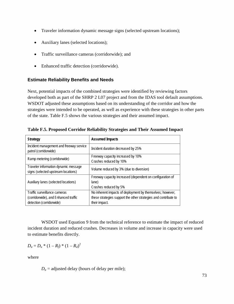
• Traveler information dynamic message signs (selected upstream locations);

• Auxiliary lanes (selected locations);

• Traffic surveillance cameras (corridorwide); and

• Enhanced traffic detection (corridorwide).

Estimate Reliability Benefits and Needs

Next, potential impacts of the combined strategies were identified by reviewing factors developed both as part of the SHRP 2 L07 project and from the IDAS tool default assumptions. WSDOT adjusted these assumptions based on its understanding of the corridor and how the strategies were intended to be operated, as well as experience with these strategies in other parts of the state. Table F.5 shows the various strategies and their assumed impact.

Table F.5. Proposed Corridor Reliability Strategies and Their Assumed Impact



Ramp metering (corridorwide) Freeway capacity increased by 10% Crashes reduced by 10%

Traveler information dynamic message signs (selected upstream locations) Volume reduced by 3% (due to diversion)

Auxiliary lanes (selected locations) Freeway capacity increased (dependent on configuration of lane) Crashes reduced by 5%

Traffic surveillance cameras (corridorwide), and Enhanced traffic detection (corridorwide)

No inherent impacts of deployment by themselves; however, these strategies support the other strategies and contribute to their impact.

WSDOT used Equation 9 from the technical reference to estimate the impact of reduced incident duration and reduced crashes. Decreases in volume and increase in capacity were used to estimate benefits directly.

Da = Du * (1 – Rf) * (1 – Rd)2

where

Da = adjusted delay (hours of delay per mile); 73

Du = unadjusted (base) incident delay from the IDAS incident delay look-up tables (hours of delay per mile);

Rf = reduction in incident frequency expressed as a fraction (with Rf = 0, meaning no reduction, and Rf = .30, meaning a 30% reduction in incident frequency); and

Rd = reduction in incident duration expressed as a fraction (with Rd = 0, meaning no reduction, and Rd = .30, meaning a 30% reduction in incident duration).

Table F.6 shows how the improvements reduce recurring and incident delay while improving mean TTI to below the thresholds for all segments. Corridorwide, the average travel time is only 15% longer than the free flow travel time and is considered reliable.

Table F.6. Reliability Benefits of Proposed Improvements


Recurring Delay (hours)

Incident Delay (hours)

Mean TTI 95th Percentile TTI

Segment 1 (NB) 165.34 339.2 1.28 1.90 Segment 2 (NB) 130.05 548.5 1.58 2.68 Segment 3 (NB) 117.09 387.8 1.31 1.99 Segment 1 (SB) 217.63 30.9 1.18 1.59 Segment 2 (SB) 99.35 258.5 1.33 2.04 Segment 3 (SB) 110.16 196.6 1.20 1.67 Corridor Total 839.62 1761.5 1.30 1.95

The proposed array of investments eliminates the reliability deficiencies in the corridor. As such, these investments can be considered needs in this corridor. The analysis showed that a relatively low-cost set of improvements, relative to major capacity enhancements in the corridor, could improve travel time reliability in the corridor. These enhancements included incident management, ramp metering, auxiliary lanes, traffic surveillance, and traveler information strategies. The TTI for the corridor with the combination of improvements deployed was estimated at 1.30. This represents a nearly 20% reduction in the index and a significant improvement in reliability.

F.5 Conclusions/Lessons Learned

The case study was successful in demonstrating how agencies can use sketch planning methods to assess the reliability impacts for a package of operations strategies within a corridor and then advance these projects into the region’s Long-Range Transportation Plan. The case study demonstrated the following:

74

• The process for collecting data and selecting appropriate analytical techniques from among several available options.

• How to divide the entire corridor into subsections. This allowed the analysis to be completed in a timely and resource-conscious manner without washing out the differences in performance that would have likely occurred if the corridor was treated as a whole.

• How to identify reliability deficiencies in a corridor using reliability thresholds.

• How a relatively low-cost set of operations investments can improve travel time reliability in a corridor.

• How agencies can apply sketch planning methods using travel demand model data and the SHRP 2 L03 data-poor reliability prediction equations within a spreadsheet environment.

Lessons learned include the following:

• Although not performed in this analysis, the approach could be easily modified to evaluate the likely reliability impact of individual strategies or different combinations of strategies, as opposed to the entire range of all proposed enhancements.

• If the analysis were to be conducted on a larger scale, involving a much greater number of individual links, it might be useful to integrate some of the analysis processes (e.g., looking up and applying incident-related delay factors) directly within the travel demand model routine to streamline the process and minimize the exchange of data.

75

case studies in using reliability performance measures in...

Documents