capturing design process information and rationale to ...€¦ · web viewdesign analysis...

Capturing Design Process Information and Rationale to Support Knowledge-Based Design and Analysis Integration

Design Analysis Integration LexiconGaTech Project #B-01-691

August 3, 2004

Submitted to:National Institute of Standards and Technology

Gaithersburg, MD

Technical Point of Contact:Steven R. [email protected]

+1-301-975-3524

Prepared by:1Manufacturing Research Center

2G.W. Woodruff School of Mechanical Engineering

Georgia Institute of Technology (GIT)Atlanta, Georgia USA

http://www.marc.gatech.edu/

Technical Points of Contact:Russell S. Peak 1 (PI)

[email protected]+1-404-894-7572

Gregory M. Mocko2 (Graduate Research Assistant)

[email protected] Bajaj2 (Graduate Research Assistant)

[email protected] Kim2 (Graduate Research Assistant)

[email protected]+1-404-385-1674

Georgia Tech Contracting Organization:Office of Sponsored Programs

Georgia Tech Research Corporation (GTRC)http://www.osp.gatech.edu

http://www.osp.gatech.edu/

mailto:[email protected]




http://www.marc.gatech.edu/


Design Analysis Integration Lexicon

PURPOSE

This document serves to enlist the definitions associated with the design-analysis integration and MRA implementation and architecture development efforts at Georgia Tech. The overarching goal in this research is towards a unified view of design-analysis integration in the context of product design at Georgia Tech. Based on this view, we leverage from other current research in the areas of product design, information management, product modeling, simulation-based design, and design and analysis integration efforts. In this context, engineering analysis means simulation of the physical behavior of a product artifact for a particular problem scope and domain.

A secondary goal is to formulate a better understanding of engineering design and analysis. A common view of design-analysis integration is the closer association between traditional design tools, such as computer-aided design (CAD) tools and computer-aided engineering tools (CAE) such as finite element analysis (FEA). This notion can be somewhat limiting. The extended approach in this research is toward the integration of engineering models throughout the life-cycle of the product. A subset of the models that are integrated over the life cycle of the product are design and analysis (simulation) models. The research advances and contributions made from DAI research should be extended to capture additional engineering model associations. In closure, the goals in this work are the following:

Review and develop a formal lexicon based on existing concepts that have been identified and/or addressed in DAI research in the EIS Lab

Identify the additional concepts that must be incorporated and considered in this work to generalize the research efforts towards engineering models associativity

Critically evaluate the current state of technology development and implementation to identify areas of opportunistic research.

The research presented in this document is primarily in the context of the Multi-Representation Architecture (MRA).

i


TABLE OF CONTENTS

PURPOSE..........................................................................................................................I

TABLE OF CONTENTS.....................................................................................................II

1 GENERAL DEFINITIONS FOR DESIGN ANALYSIS INTEGRATION.............................1

1.1 ANALYTICAL MODEL....................................................................................1

1.2 ANALYSIS MODEL.........................................................................................1

1.3 ANALYTICAL VARIABLES.............................................................................1

1.4 ANALYSIS IDEALIZATION..............................................................................1

1.5 REPRESENTATION.........................................................................................1

1.6 INFORMATION MODEL..................................................................................1

1.7 ROUTINE ANALYSIS MODEL..........................................................................2

1.8 ADAPTIVE ANALYSIS MODEL........................................................................2

1.9 ORIGINAL ANALYSIS MODEL........................................................................2

1.10 ASSOCIATIVITY.............................................................................................2

1.11 PRODUCT-ANALYSIS TRANSFORMATIONS (PAT).........................................2

1.12 ANALYSIS-ANALYSIS TRANSFORMATIONS....................................................2

1.13 IDEALIZATION...............................................................................................3

1.14 DIMENSIONAL REDUCTION...........................................................................3

1.15 GEOMETRIC SYMMETRIES............................................................................3

1.16 FEATURE REMOVAL.....................................................................................3

1.17 DOMAIN ALTERATION..................................................................................3

1.18 PHENOMENON REMOVAL.............................................................................3

1.19 PHENOMENON REDUCTION...........................................................................3

1.20 PHENOMENON IDEALIZATIONS.....................................................................3

1.21 BOUNDARY CONDITION IDEALIZATIONS......................................................4

1.22 MATERIAL IDEALIZATIONS...........................................................................4

1.23 SYNTHESIS....................................................................................................4

1.24 PRODUCT VARIABLES...................................................................................4

1.25 PRODUCT IDEALIZATION RELATIONS............................................................4

1.26 HOMOGENEOUS DATA EXCHANGE...............................................................4

1.27 HETEROGENEOUS DATA EXCHANGE............................................................4

1.28 MULTI-FIDELITY HETEROGENEOUS TRANSFORMATIONS.............................5

ii


1.29 OBJECT-ORIENTED MODELING......................................................................5

1.30 NON-CAUSAL MODELING..............................................................................5

1.31 EXPLICIT REPRESENTATION OF IDEALIZATION KNOWLEDGE........................5

1.32 REUSABLE IDEALIZATIONS...........................................................................6

1.33 MULTI-FIDELITY IDEALIZATIONS..................................................................6

1.34 LATE-BOUND OPERATIONS...........................................................................6

1.35 PRODUCT DOMAIN-INDEPENDENT................................................................6

1.36 COMPUTER INTERPRETABLE FORM..............................................................6

1.37 PRODUCT VARIABLE.....................................................................................6

1.38 DESIGN SYNTHESIS.......................................................................................6

1.39 COMPLEXITY LEVEL.....................................................................................6

1.40 VARIABLES...................................................................................................7

1.41 SUBSYSTEM..................................................................................................7

1.42 SCOPE...........................................................................................................7

1.43 GRAPH..........................................................................................................7

1.44 SIMPLE GRAPH.............................................................................................7

2 COB SPECIFIC IMPLEMENTATION DETAILS..........................................................7

2.1 CONSTRAINED OBJECT REPRESENTATION.....................................................7

2.2 OVERVIEW OF COB REPRESENTATION........................................................7

2.3 COB DEFINITION LANGUAGES.....................................................................8

2.4 COB STRUCTURE DEFINITION LANGUAGE (COS LANGUAGE)....................8

2.4.1 COB Relation...............................................................................9

2.4.2 COB Sets....................................................................................10

2.5 COB INSTANCE DEFINITION LANGUAGE (COI LANGUAGE)......................10

2.6 COB GRAPHICAL REPRESENTATIONS........................................................11

2.6.1 Basic Object-Relationship (EXPRESS-G) Diagram Notation. .11

2.6.2 Basic Constraint Network Diagram Notation............................12

2.6.3 Basic Constraint Schematic Diagram Notation.........................13

2.6.4 Additional Constraint Schematic-I Notation (COI)...................13

2.6.5 Extended Constraint Graph/Network -S Diagram Notation......14

2.7 COB META INFORMATION MODEL............................................................18

2.8 COB PROTOCOL.........................................................................................19

2.8.1 COB Creation.............................................................................19

iii


2.8.2 COB Usage................................................................................21

2.8.3 COB Storage..............................................................................24

2.9 WIRTH SYNTAX NOTATION FOR COB DEFINITION LANGUAGES25

2.10 BASIC LANGUAGE ELEMENTS.....................................................................26

2.10.1 Character classes........................................................................26

2.10.2 Remarks.....................................................................................26

2.10.3 Reserved words..........................................................................26

2.10.4 Identifiers and Interpreted Identifiers........................................26

2.11 LITERALS....................................................................................................26

2.11.1 Real literal..................................................................................26

2.11.2 String literal...............................................................................26

2.11.3 Unknown literal.........................................................................26

2.12 COB INSTANCE DEFINITION LANGUAGE ( COI ).......................................27

2.12.1 Data............................................................................................27

2.13 COB SCHEMA DEFINITION LANGUAGE (COS)..........................................27

2.13.1 Data types...................................................................................27

2.13.2 Declarations...............................................................................28

2.14 SUBTYPES ( COB_SUBTYPE ).......................................................................28

2.15 ANALYSIS-ORIENTED PRODUCT MODEL (AOPM).....................................29

2.16 PRODUCT MODEL (PM)..............................................................................29

3 ABB SPECIFIC TERMINOLOGY............................................................................29

3.1 ANALYSIS BUILDING BLOCK (ABB)..........................................................29

3.2 GENERIC ABB............................................................................................29

3.3 PRODUCT SPECIFIC ABB............................................................................29

3.4 ANALYTICAL PRIMITIVES...........................................................................29

3.5 ANALYTICAL SYSTEM.................................................................................30

4 APM SPECIFIC TERMINOLOGY............................................................................30

4.1 APM INSTANCE..........................................................................................30

4.2 ANALYZABLE PRODUCT MODEL (APM)....................................................30

4.3 APM INFORMATION MODEL......................................................................30

4.4 APM DOMAIN INSTANCE...........................................................................30

4.5 APM PRIMITIVE ATTRIBUTES....................................................................30

4.6 SUPERTYPE_DOMAIN..................................................................................30

iv


4.7 SET OF APM COMPLEX DOMAINS.............................................................30

4.8 APM ATTRIBUTES......................................................................................30

4.9 APM DOMAIN INSTANCES.........................................................................31

4.10 APM OBJECT DOMAIN INSTANCE..............................................................31

4.11 APM DOMAIN SETS AND APM SOURCE SETS...........................................31

4.12 APM SOURCE SET......................................................................................31

4.13 APM SOURCE SET LINKS...........................................................................31

4.14 APM PRODUCT ATTRIBUTES.....................................................................31

4.14.1 APM Essential Product Attributes.............................................32

4.14.2 APM Redundant Product Attributes..........................................32

4.15 APM IDEALIZED ATTRIBUTES....................................................................32

4.16 ENVIRONMENTAL ATTRIBUTES...................................................................32

4.17 BEHAVIORAL ATTRIBUTES..........................................................................32

4.18 APM RELATIONS........................................................................................32

4.18.1 Set of APM Relations................................................................32

4.18.2 APM Product Relation...............................................................33

4.18.3 APM Product Idealization Relation...........................................33

5 SMM SPECIFIC TERMINOLOGY...........................................................................33

6 CBAM SPECIFIC TERMINOLOGY.........................................................................33

6.1 PRODUCT MODEL-BASED ANALYTICAL MODEL (PBAM)...........................33

7 MANUFACTURABLE PRODUCT MODEL SPECIFIC TERMINOLOGY (MPM)..........33

7.1 MANUFACTURABLE PRODUCT MODEL.......................................................33

8 PRODUCT MODEL SPECIFIC TERMINOLOGY........................................................33

8.1 PRODUCT MODEL (PM)..............................................................................33

9 Bibliography.......................................................................................................34

v


1 GENERAL DEFINITIONS FOR DESIGN ANALYSIS INTEGRATION

This section contain concepts for the general research area of design analysis integration

1.1 Analytical model

An engineering approximation of physical behavior in exact form

Example: A spring system.

FFk

L

deformed state

Lo

L

x2x1

Figure 1 - Spring system analytical equation

The spring equation is: xkF

The force, F, exerted by the spring is proportional to the spring constant, k, and the displacement, x, of the spring. The equation is the exact form of the analytical model. This analytical model may be a simplified abstraction of the actual behavior of the spring. The equation is only an approximation of the actual behavior of the spring.

1.2 Analysis model

An analytical model or an approximation of the analytical model. The analysis model may be the exact or an approximation of the analytical model. Several different types of approximation techniques may be employed and several different analysis models may be utilized

1.3 Analytical variables

A variable that is used in the analysis relation.

1.4 Analysis idealization

A transformation from the physical situation into analysis attributes. The analysis idealization is the natural direction of the transformation.

1.5 Representation

A computable approximation of the real world for an intended purpose there may be more than one way to represent reality. The intended purpose of the representation determines what type of information is needed for the representation. The representation must be able to be implemented in a computer.

1.6 Information model

A formal (being in accordance with rules explicitly established prior to use) model (an abstract description) of a bounded set of facts, concepts, or instructions to meet a specified requirement.

1


1.7 Routine analysis model

An established analysis model that is repeatedly used for a specific type of product, but not a specific product instance. Routine analysis is the process of using routine analysis models – using proven models on new instances . The variables and parameters of the product remain fairly well known as do the relations. However, the value of each variable is dependent on the product instance. Routine analysis does not imply the models are simplistic. The models can be quite complex. However, the users of the models must know the limitations of the models

1.8 Adaptive analysis model

Developed by adapting some aspect of a routine analysis model. Each time a “new” model is created, the results must be validated to ensure the analysis model is correct. Routine analysis models can be extended for slightly different analysis needs.

1.9 Original analysis model

An entirely new model that replaces an existing analysis model for a given type of product or analyzed a new type of problem.

Table 1 - Types of analysis

Class Task Performer Task Task Output

Routine Product Designer Use established analysis model repeatedly.

Analysis Results,Design Changes

Adaptive Product Designer or Engineering Analyst

Extend routine model for same product type.

Extended Analysis Model, Sample Results

Original Engineering Analyst and Experimentalist

Develop new analysis model for same / new product type.

New Analysis Model, Sample Results

1.10 Associativity

Linking of analysis models with product models. The data in the analysis must be linked to the data of the product

1.11 Product-analysis transformations (PAT)

The linkages that are “hard-wired” between the product representation and the analysis representation. These linkages may also be known as extraction of information. The linkages are vital. The linkages should support bi-direction flows according to the PAT.

The two types are analysis idealizations and design synthesis operations. A linkage that is between one or more product variables and one or more analytical variables. The PATs are used to link the product variables with some of the analytical variables

1.12 Analysis-analysis transformations

A linkage that relates two or more analytical variables, emphasis is placed on linkages between variables

2


1.13 Idealization

To idealize is to construct an abstracted model of the real system that will admit some form of mathematical analysis (Shigley and Mischke 1989). Most frequently, idealization refers specifically to the transformations that are applied to the design representation of a part, which is already an idealized version of the “real” or “physical” part in that the design representation is a model of the typical actual part Idealizations are applied to design information because most problems contain complexities that render numerical simulation difficult or impossible to analyze. Finn provides the following categorization of engineering idealizations1:

1.14 Dimensional Reduction

Involves reducing the degree of spatial analysis or time analysis. Spatial analysis may involve reduction from 3-dimensional to 2-dimensional or 1-dimensional analysis. Time analysis may involve reducing a transient analysis to a quasi-static or steady state analysis.

1.15 Geometric Symmetries

Involves removing redundant domains by identifying spatial symmetries and applying compensatory boundary conditions.

1.16 Feature Removal

Involves removing some engineering feature that is not expected to contribute significantly to the overall analysis results (for example a small hole or a fin).

1.17 Domain Alteration

Involves changing some aspect of the spatial domain so that the analysis is simplified (for example, modeling a thin aerofoil as a thin plate).

1.18 Phenomenon Removal

Involves the removal from analysis of complete phenomena based on the decision to ignore the effect of that phenomenon (for example, ignoring stress effects within the physical system).

1.19 Phenomenon Reduction

Applies to situations where a multi-component phenomenon exists and a particular component is removed is removed because its significance is judged to be of minor importance (for example, removing radiation analysis from a heat transfer problem).

1.20 Phenomenon Idealizations

Involves the use of mathematical expressions to describe the system phenomena. For example, in fluid analysis, a number of mathematical equation models are available to solve for flow analysis: parallel flow can be modeled using the full Navier Stokes equations or a Couette flow model.

1 Finn distinguishes between simplifications and idealizations . In the list below, he considers the first six operations simplifications and the last three idealizations. For the purposes of this discussion, a simplification will be considered as a type of idealization.

3


1.21 Boundary Condition Idealizations

May involve applying a mathematical equation to model a boundary condition that does not perfectly represent the physical boundary conditions. For example, in heat transfer modeling, a non-ideal surface may be modeled as a black body or gray body surface.

1.22 Material Idealizations

generally involve the use of idealized material laws to model some complex material behavior. For example, modeling an expected non-linear material response using a linear approximation function.

1.23 Synthesis

Synthesis is the opposite of idealization; the act of “appearing as a material form or taking substantial shape”, that is, going from an abstract or ideal representation to a physical representation. Effectively, synthesis is performed in three steps: the first is to decide on the variables (primitive or complex) from the design representation of the part that are going to be populated with values. The second step is to assign values to these variables. The third step is to use this populated design representation to actually create or manufacture the physical part. The assignment of values to the design variables is normally based on the results of engineering analyses, but it could possibly be based on rules-of-thumb, experience or even arbitrary judgment.

1.24 Product variables

The design representation of a product is expressed exclusively in terms of product variables. Idealized variables whereas analysis representations are expressed as a combination of product variables and idealized variables.

1.25 Product idealization relations

Product and idealized variables are related by product idealization relations. When these product idealization relations are used to obtain idealized variables from product variables (that is, in their “forward” form) they are called idealizations. When they are used in the “reverse” direction, that is, to obtain product variables from idealized variables, they are called synthesis relations.

In the context of design-analysis integration, idealization and synthesis characterize the bi-directional nature of the design-analysis process:

1.26 Homogeneous Data Exchange

Data exchange that occurs between systems that are similar in scope and semantics, hence mostly requiring syntactic translation of the data.

1.27 Heterogeneous Data Exchange

Is caused by the large gap in scope and semantics that exists between design and analysis representations, which requires a syntactic and a semantic transformation of the data being exchanged. A major issue between design and analysis representations

4

Greg Mocko, 08/22/04,

These synthesis relations are called mapping in Fenves terminology


1.28 Multi-Fidelity Heterogeneous Transformations

The term Multi-Fidelity Heterogeneous Transformations can be used to convey this notion of different levels of detail of the models. The following figure depicts the notion of multi-fidelity idealizations.

Flap Link

Multi-fidelityIdealizations FEA-Based

Tension Analysis

Formula-Based Tension Analysis

Simple CrossSection

Detailed CrossSection

MultipleUses

criticalcrosssection

Figure 2 - Multi-Fidelity Analysis

1.29 Object-oriented modeling

Makes it possible to create physically relevant and easy-to-use components, which are employed to support hierarchical structuring, reuse, and evolution of large and complex models covering multiple technology domains.

1.30 Non-causal modeling

Modeling is based on equations instead of assignment statements as in traditional input/output abstractions. Equations do not specify which variables are inputs and which are outputs, whereas in assignment statements variables on the left-hand side are always outputs (results) and variables on the right-hand side are always inputs. Thus, the causality of equations-based models is unspecified and fixed only when the equation systems are solved (this is called non-causal modeling). Direct use of equations significantly increases reusability of model components, since components adapt to the data flow context in which they are used (in other words, they can be used with multiple input/output combinations of data). This generalization enables both simpler models and more efficient simulation.

1.31 Explicit representation of idealization knowledge

The transformations required to obtain the values of idealized attributes from design or product attributes are not explicitly defined anywhere. As a consequence, they end up buried inside the code of the analysis applications making it difficult to reuse or modify them. The APM Representation should provide the necessary constructs for defining idealized attributes or features of the part as well as the mathematical relations that define how these idealized attributes are derived from the “real” or “manufacturable” attributes of the part. These definitions should be formally captured as part of the analyzable product model itself.

5


1.32 Reusable idealizations

Idealized attributes and product idealization transformations should be defined in such a way that they can be used by potentially more than one analysis application (in other words, be reusable).

1.33 Multi-fidelity idealizations

Different levels of precision by using more or less accurate idealizations of a feature. For instance, a coarse analysis may only require a simple approximation of a feature, whereas a more precise analysis would require a more detailed (and, consequently, more computationally-demanding) version.

1.34 Late-bound operations

Late-bound operations are designed to manipulate information without previous knowledge of the domain-specific structure of the data. It should be possible to reuse these operations in a range of application domains without having to modify or customize them.

1.35 Product domain-independent

Independent from any particular product domain or industry (for example, airplane structures, printed wiring assemblies, etc.). In other words, it should be generic. The constructs defined in this representation should not be expressed in terms of any particular domain. The APM Representation should serve as a “template” for creating domain-specific analyzable product models.

1.36 Computer Interpretable Form

Computer-interpretable language for defining analyzable product models. A computer program should be able to parse this definition and create a corresponding representation of the analyzable product model in memory that can be accessed and manipulated by analysis applications. This computer-interpretable language must be easy to understand by humans without extensive knowledge of its syntax.

1.37 Product variable

A variable that the designer would specify in order to fully define the product. product variables cannot be directly used in the analysis model (AKA: product parameter)

1.38 Design synthesis

Generate product information by adding detail to analysis output or transforming them. There may be two different types of synthesis activities 1) activities that modify the basic working principles of the design and 2) activities that actually generate more information and feature on the design side. The design syntheses are typically under constrained relations.

1.39 Complexity level

Analysis models may be of varying complexity. This is related to the simplicity or abstraction of the model. For example, the model may be equations-based or may rely on complex finite element analysis.

6


1.40 Variables

Variables are the input and the output of the analysis and design model. They are used for exchange with other models.

1.41 Subsystem

is another view of an analytical building block object that shows related variables in the object to fulfill a particular purpose. A subsystem may be used in a graph of another object. subsystems can be nested arbitrarily deep

1.42 Scope

The context in which the product parameter are valid. A variable can be known in one subsystem and also in the other, but not be the same variables.

1.43 Graph

A triple ),,( EVG where V and E are finite set and O is a function

1.44 Simple Graph

A graph whose edges are undirected, that does not have multiple edges between the same two vertices, and that does not allow edges from a vertex to itself (Rosen 1995)).

2 COB SPECIFIC IMPLEMENTATION DETAILS

The COB specific implementation details are organized in the context of MRA.

Solution Method Model

ABB SMM

Analysis Building Block

Context-Based Analysis Model

SMMABBAPM ABB

CBAM

APM4

Design Tools Solution Tools

Printed Wiring Assembly (PWA)

Solder Joint

Component

PWBSolder Joint

Component

PWB

body3body2

body1

body4

T0

body3body2

body1

body4

T0

Printed Wiring Board (PWB)

SolderJointComponent

Printed Wiring Board (PWB)

SolderJointComponent

AnalyzableProduct Model

3

2

1

Figure 3 –Multi-Representation Architecture

Terminology and concepts are then presented for each specific type of COB, including CBAMs, ABBs, APMs, and SMMs.

2.1 Constrained object representation

The four main components are the COB Meta Information Model, the COB Protocol, the COB Definition Languages, and the COB Graphical Representations.

2.2 Overview of COB Representation

COB representation consists of the four main components.

7


COBRepresentation

DefinitionLanguages

MetaInformation

Model

GraphicalRepresentations

Protocol

(section 4.2) (section 4.3)

(section 4.4)

Figure 4 - COB representation components

2.3 COB Definition Languages

The COB Representation includes two definition languages called the COB Structure Definition language (COS language) and the

2.4 COB Structure Definition Language (COS language)

The COS language is used to define the structure of COBs, also known as a COS model. The COS model describes a domain-specific model and is considered to be a “template” of potentially many COI model. The COS language is developed based on the general purpose STEP EXPRESS language (ISO 10303-11). EXPRESS is an object-flavored information model specification language that is developed in order to enable the writing of formal information models describing mechanical products. EXPRESS is the one of the technologies that has been developed as part of the STEP standard for product data exchange.

The EXPRESS language was extended and simplified to establish the COS language that is specifically tailored for design-analysis integration.

To define attributes with symbols. Analysis attributes used in relations are usually defined with symbols such as “L = k * ΔL” rather than “length = spring constant * deformation”.

To represent relations between primitive attributes. EXPRESS language provides similar capability with WHERE rule, but that is for conformance checking between primitive attributes and is not suitable for calculation of unknown variable values in a constraint graph base way. To define and categorize attributes, relations, and cobs specifically tailored for design and analysis integration (DAI). For example, idealized attributes. For flexibility in defining future extensions tailored to DAI.

The main elements of the COB Structure (COS) are schema, cob sets, cobs, and cob set links. The cobs, like entities in EXPRESS, are the building block of COS. A COS is built from cobs, like entities in EXPRESS, and each cob (except primitive ones) contains attributes to represent its essential properties and relations to specify mathematical constraints among its primitive attributes and sub attributes. An attribute declaration consists of the name and data type of the attribute. The data type specifies the type of value that the attribute has when it is instantiated. It may be a pre-defined primitive cob (REAL or STRING), a complex cob (a cob that has attributes and/or relations), or an aggregate where members are primitives or complex cobs.

8


2.4.1 COB Relation

A relation declaration consists of a relation identifier (name) and a mathematical expression. A relation is usually constraint-based (i.e., multi-directional) and used to calculate unknown variable values.

2.4.1.1 Extended Aggregate Relation

A relational expression can be constructed with aggregate instance(s). For example, the following defines a potential mathematical relation between the aggregate elements in aggregate primitive cob a4 from cob a abover3: “<a4[0]> == <a4[1]> * a4[2]”;

A relation may include the following aggregate operations the utilize all aggregate members: Summation, Maximum, or Minimum. For example, the following relation:r3: “<a1> == <a4.SUM>”;

defines that the summation of the values in primitive aggregate a4 must be equal to a1 no matter how many instances of a4 are provided. Also, the aggregate operation can be defined among elements in a complex aggregate such asr4: “<a1> == <a6.MIN[b1]>”;

This relation defines that the minimum of value of the attribute of all members of b1 in complex aggregate a6 must be equal to a1. These extended relations with aggregate operations so that they are now multi-directional.

2.4.1.2 Uni-directional Relation (ONEWAY)

When a relation is declared ONEWAY, the attribute in its left-hand-side will always be output and the attributes in its right-hand-side are inputs. For example, consider the following relation. r5: “<a> == <b> + <c>” ONEWAY;

It means a is always output and b and c are always inputs. This capability has been developed primarily to support a special kind of uni-directional relation that wraps an external tool to obtain a variable value of output. See the following example.“<e>==CobExternalToolFunction[T_name,F_name,{<a>,<b>,<c>}]” ONEWAY;

The first string between brackets ([ ]) indicates the external tool name, and the second string indicates the external file name. The variables listed between curly-brackets ({ }) are input variables. This particular relation runs the finite element tool (FE), called "T_name" to determine variable value e with a FE model created with a pre-prepared parameterized template defined in the file called "F_name" with input values of a, b, and c. The left-hand-side variable is always output, as tool like FE ANSYS typically have a fixed natural output direction (e.g., calculating stress given material, geometry, and loads as inputs).

2.4.1.3 Conditional Expressions

Another extension is three "if" control statement relations. Their forms are

9


"IF_STRING (condition): relation"

"IF_TYPE (condition): relation"

"IF_AGGREGATE_SIZE (condition): relation".

The condition is a Boolean expression. If condition is true, then is included in the constraint network. Relational operators are used in conditions. IF_STRING utilizes the "Equal to (==)" operator to check the value of string-primitive attributes. For example, "IF_STRING (ball_type = grid): <number_of_balls> == <balls_in_x> * <balls_in_y>" checks the string value of ball_type attribute. If its value is grid, the relation followed by the condition is included. IF_TYPE also uses "Equal to (==)" operator to check complex cob's types. For example, "IF_TYPE (package == ebga): "mold.height == package.height" checks if the type of the complex attribute package is ebga. IF_AGGREGATE_SIZE may use "Equal to (==)", "Greater than (>)", "Less than (<)", "Greater than or equal to (>=)", or "Less than or equal to (<=)" operators. It checks the size of aggregates (i.e., the number of members in an aggregate).

2.4.1.4 Inherited Relation Redefinition

When a cob is a subtype of another cob, the subtype inherits all attributes and some relations from its supertype. However, relation will not be inherited when its relation name in the subtype is the same as that in its supertype, thus providing overwriting capability of relations.

2.4.2 COB Sets

Collections of similar cobs are grouped into cob sets within a given cob schema. Each cob set contains a root cob to specify a root of the hierarchy tree. How cobs in the different cob sets are related is defined in link definitions. The cob sets and their links construct the top building block called schema. The following example shows the concepts. Schema test has two cob sets set_a and set_b with root cobs, a and b, respectively. Those two cob_sets are linked together to form a linked cob with the equality relation define between LINK_DEFINTION and END_LINK_DEFINTION. Enhanced Structure Reusability (USE_FROM)

2.5 COB Instance Definition Language (COI language).

The COI language is used to define an instance of the COS, also known as a COI model. A COI model is a collection of COBs that describes a domain-specific data. A COI definition is stored in a text file known as a COI file. The COB Instance Definition language (COI) has similar capability with the general-purpose STEP Part21 File format (ISO 10303-21). Both COI and STEP Part21 may be used to define constrained objects. However, STEP Part21 is developed for the purpose of exchanging data among computer systems and it lacks in friendliness to humans: lacks in readability, and creation of data files is tedious. Thus, the COI is developed to overcome such shortcomings. The main elements of a COB Instance (COI) model are an instance of root COB and a list of primitive COBs belonging to the root COB. The COI definition syntax starts with DATA syntax and ends with END_DATA. More than one COI may be defined in the same COI file. Each COI is enclosed between INSTANCE_OF and END_INSTANCE keywords. The INSTANCE_OF keyword is followed by a root cob instance name. Between INSTANCE_OF and END_INSTANCE, there is a list of definitions describing cob

10


primitive attribute values. Note that a COI definition does not require that all primitive attributes defined in its COS be listed here; the only required attributes are the inputs and the primary desired output.

2.6 COB Graphical Representations

These visual forms aid human interpretation of the COB Representation concept. Both COS and the COI have graphical representations to aid human interpretation of the COB models. Each of these graphical representations conveys a certain aspect of the COB better than the others. For example, the object relationship diagram (EXPRESS-G) shows the generalization and specialization nature of objects, but it does not depict the mathematical relations among their attributes; mathematical relations can be observed from a constraint schematic diagram. The main COB graphical representations are:

Object-Relationship diagram

Constraint network diagram

Constraint schematic diagram

2.6.1 Basic Object-Relationship (EXPRESS-G) Diagram Notation

An object-relationship diagram uses EXPRESS-G, which is part of the STEP standard (ISO 10303-11 1994) for the graphical representation of the EXPRESS lexical language. The object relationship diagram shows “the is-a relationship” in bold lines and “the part-of relationship” in thin lines. Entity is used synonymously with COB.

2.6.2 Basic Constraint Network Diagram Notation

A constraint network diagram is used to represent how COB attributes and relations are interconnected. This Diagram is useful for the following reasons:

11


To visualize how a change in an attribute value affects the other attribute values.

To determine which relations should be used to build the system of equations to solve for an attribute value.

To figure out possible input/output combinations for attributes.

To visualize which relations are multi-directional (MULTI-WAY) and which relations are uni-directional (ONEWAY).

A "full attribute name" is obtained by concatenating the attribute from the root cob to the terminal attribute in its hierarchy tree.

A MULTI-WAY connector (default type of connector) is for a relation that does not define which attributes are inputs or outputs. For example if the “R4” relation is stated as “A.a1 = A.a2 + A.a3”, the relation has three possible input/output combinations: “A.a1” is output and “A.a2” and “A.a3” are inputs, “A.a2” is output and “A.a1” and “A.a3” are outputs, and “A.a3” is output and “A.a1” and “A.a2” are inputs.

A ONEWAY connector is for a relation that is defined with a specified input/output combination. For example if the “R1” relation is defined as a ONEWYA relation where “A.a1 = A.a2 + A.a3”, then “A.a1” is always output and “A.a2” and “A.a3” are always inputs.

A constraint network is an alternate way to represent COB Relations. In a constraint network, variables and relations are represented as vertices of a simple graph. Each node in a constraint network may be either a variable or a relation. Variables can only be connected to relations and relations can only be connected to variables. This representation allows to determine what variables are affected by the change in value of a given variable, or what relations are required to calculate the value of a given variable.

12


2.6.3 Basic Constraint Schematic Diagram Notation

Figure 5 - Constraint Schematic-S Notation (COS)

2.6.4 Additional Constraint Schematic-I Notation (COI)

200 lbs

30e6 psi

X

Relation r1 is suspendedX r1

100 lbs

Equality relation is suspended

a

b

c

100 lbs Primary Input(Input 10 lbs)

a

Intermediate Input(Input 10 lbs)

Intermediate Output(Result = 30e6 psi)

Primary Output(Result = 200 lbs)

13


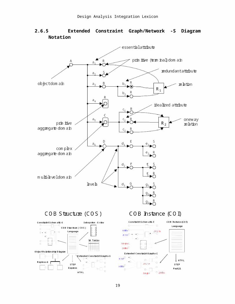
2.6.5 Extended Constraint Graph/Network -S Diagram Notation

Figure 6. COB Modeling Views

14


Figure 7 - Object Relationship Diagram (EXPRESS-G).

The constraint network shown is a "flattened" view of the constraint schematic view explained next.

spring2.spring_constant

spring2.total_elongation

bc4

spirng1.spring_constant

spring1.Total_elongation

spring1.undeformed_length

r2

spring1.length

r3

load

r2

spring2.length

r3

spring2.force

deformation1 deformation2

bc5

spring1.force

spring2.undeformed_lengthbc6

bc3

r1

spring1.start

spring1.end

r1

spring2.end

spring2.start

bc2

bc1

Figure 8 - Constraint network-S diagram

A COB subsystem view, where a high-level object is wrapping one or more lower-level objects and/or other sub-systems, may be included in a COB constraint schematic2. It is an abstraction view of a COB that hides unnecessary details from users. The full constraint network is present and active in subsystems no matter which variables are shown on a subsystem view. A line connecting attribute(s) means equality and the constraint schematic shows only system level relations that are defined in the COB structure definition of the two-spring system.

2 Constraint schematic diagrams were first introduced in [2] to represent Analysis Building Blocks and Product Model-Based Analysis Models.

15


Spring

LL

Fk

1x L0

2x

Figure 9 Spring -subsystem-S view

bc1

spring 1

2u

spring 2

1u

PSpring

Elementary

LL

Fk

1x L0

2x

122 uLu

bc2 bc3

bc4

bc6

SpringElementary

LL

Fk

1x L0

2x

bc5

011 x

spring2spring1

L10

k1

L1

L1

L20

k2

x21

x22

F2

L2

L2

F1

bc4

r12

r13

r22

r23

bc5bc6

bc3

r11 r21

bc2

bc1

u1 u2

P

x11

x12

Constraint Schematic-S

Constraint Network-S

Figure 10 - Two-spring system - constraint schematic-S diagram (with spring) with constraint network-S

L

L

Fk

u n d e fo rm e d le n g th ,

s p r in g c o n s ta n t , fo rc e ,

to ta l e lo n g a tio n ,

1x

Lle n g th ,0

2x

s ta rt,

e n d ,

oLLL

12 xxL

LkF

r1

r2

r3

Figure 11 - Figure Spring - constraint schematic-SSpring System

spring2

Pspring1

u1

u2

Figure 12 - Two-spring system - subsystem-S view

As mentioned before, in the constraint network lines are used to represent connection between relations and their related attributes. For example, a multi-way relation r1, <a> == <b>+<c> is depicted as below.

16


R1a

c

b

Figure 13 - Multi-way relation: constraint network-S

For a special kind of relation, a uni-directional (oneway) relation, the lines connecting attributes and relations are replaced with arrows to shows data flow directions. For example, consider a uni-directional relation, <a> == <b> + <c>. If a is output and b and c are inputs, its constraint network is depicted as below.

R1a

c

b

Figure 14 - Oneway relation: constraint network-S

The Graphical Representations mentioned in this section so far deal with the structure of COBs. Instance of COBs may be viewed with the Constraint Network Diagram-I and/or Constraint Schematic Diagram-I. Adding variable values in schema-level diagrams creates instance-level diagrams. The values enclosed by single-line boxes are inputs. If the input is assigned at the COB Structure level, the variable value has an underline (e.g., r1 relation in the two-spring system example where zero is assigned to spring1.start). Values enclosed by the double-line box are the primary desired outputs. Values without boxes are intermediate outputs whose values are found during the determination of the primary desired output(s).

Spring2 Spring1

bc4

spring_constant

total_elongation

undeformed_length

r2

lengthr3

load

r2

lengthr3

force

deformation1 deformation2

bc5

force

undeformed_length bc6

bc3

r1

start

end

r1

end

start

bc2

bc1

5.5

8.0

0

10.0 10.0

1.8183.485

10.0

9.818

9.818

1.818

6.0

8.0

9.66719.48

9.818

1.667

a. Constraint network-I diagram

17


b. Constraint schematic-I diagram

Figure -15 COB instance diagrams for a two-spring system exampleCOB Protocol

2.7 COB Meta Information Model

The information model for the COB structure and the COB instance and deals with generic aspect of the COB representation. An instance of the COB Meta Information Models defines the COS and COI and they can be accessed via COB Protocol that allows interpretation of data interactively.

GenericMetadata

GenericData

SpecificStructureData

SpecificInstanceData

COBInstanceDefinitionData

COBStructureDefinitionData

Example:

COICOICOSCOS

L

k x2F

LL

x1F 10.010.0

20.020.0

5.05.0

22.022.02.02.0

10.010.0 32.032.0

GraphicalRepresentations

Protocol

DefinitionLanguages

Meta InformationModel

Figure 16 - The COB meta information model with other components

18


2.8 COB Protocol

This section describes the major operations that compose the COB Protocol. These operations are called late-bound because they are designed to access and manipulate the COB Representation without previous knowledge the definition of domain-specific COS entities.

The following is a typical sequence of high-level tasks performed by a typical COB-based application (an application that manipulates COB using operations defined in the COB Protocol).

1) COB Creation

2) COB Usage

3) COB Storage

COB DefinitionFiles

ConstraintSolver

COB Structures

COB Instances

Constraint Network

COB basedCustom Tools

Creation• COS• COI• CNT

COB Usage• solve• change I/O• change value• activate relation

…..

Storage

Constrained Objects (COBs)

ClientApplication

M

COB Protocol

ClientApplication

MClient

ApplicationMClient

Application1

Figure 17 - High level COB protocol operations

2.8.1 COB Creation

The COB Protocol must provide a way to create cobs. First, the COS must be created in order to make available meta data that correspond to the structure of COBs (the domain–specific model template). This is done by parsing a COS model. The COS model must be linked according to what is specified by the COB Source Set links.

19


cob_a a1

a2

a3 R

S

set_a

cob_b b1

b2

S

R

set_b

R

Figure 18 - Source set link example - before link: extended constraint graph -S

The COS model has two source sets (set_a, and set_b) and one source set link (defined between the keywords LINK_DEFINITIONS and END_LINK_DEFINITIONS in the definition file). As illustrated in, the source set link links attribute a1 of domain cob_a in set_a COS with attribute b1 of domain cob_b in set_b COS. .

cob_a a1

a2

a3 R

S

set_a

cob_b b1

b2

S

R

set_b

R

link

Figure 19 - Source set link example - connecting: extended constraint graph-S

Scob_a a1

a2

a3 R

cob_bb1

b2 RR

Figure 20 - Source set link example - after link: extended constraint graph-S

2.8.1.1 COI Creation

Second, one or more COI models must be created to make the domain-specific data (instances of the COS) accessible. This is done by parsing a COI file describing a particular model using the COI language. The COI also must be linked. This operation is similar to linking the COS definition described previously. The difference is that instead of linking attributes of COB domains, this operation links instances of these attributes.

20


2.8.1.2 Constraint Network Creation

Next, an instance-based constraint network for each COI is created so that it can be used to construct simultaneous equations to solve unknown variable values. The relations of each complex cob are added to the constraint network. Each cob is identified with its full attribute name so that it will be unique within the constraint network. For example, length of spring in spring1 and spring2 instances are defined as spring1.length and spring2.length. .

As mentioned before a COI model does not need to contain all COBs defined in its corresponding COS model: all that is required are primitive attributes that are input and primary desired output3. This is because intermediate COIs, connected to these defined COIs at the constraint network level, will be automatically created during constraint network construction.

Relations with aggregate operations (SUM, MAX, and MIN) are instantiated/expanded based on aggregate instances when they are added to a constraint network. A relation such as a = b.SUM, where b is a real-primitive aggregate, is expanded to a = b[0] + b[1] + b[2] if b has three aggregate elements. A relation with MAX and MIN aggregate operations such as a = b.MAX it also instantiated in similar way. For example, if there are three b aggregate elements, the relation is instantiated as a = MAX[b[0], b,[1], b[2]]. This relation is also multi-directional. For example, if a is known to have a value of 10.0 and b[0] and b[1] are known to already be less than 10.0. Then b[2] will be set equal to 10.0. Similar instantiation is performed for the MIN operator.

b[0]

aSUM

b[1]

b[2]

Figure 21 - Constraint network-S for “a = b.SUM”

2.8.2 COB Usage2.8.2.1 Query

After constructing the cobs, the COB Protocol must provide a way to query information about the domain-specific instances (COIs) data. Any attribute of an instance is accessible via the get method with the full attribute name as its argument4. The full attribute name is obtained by concatenating the attribute names all the way up in the hierarchy tree to the cob that is receiving this method.

3 Except for aggregate instances. For example, a relation <a> = <b.MAX> to be correctly added to constraint network at least one instance of b should be defined.4 A strong typed programming language such as Java needs pre-declared variable types at compile time. In this case, these protocol operations must be modified to specify their return type (i.e., a get attribute becomes get real attribute )

21


There are two special query methods for primitive attributes (REAL and STRING) - get value and set value. Sending the method to a primitive cob or a non-primitive cob with a full attribute name as its argument permits access to its primitive values.A R

S

R

B

R

R

D

R

C

R

a1

a2

a3

a4

a5 c2

c1

c3

b1

b2

R

Rd1

d2

Figure 22 - An example COS: extended constraint network

2.8.2.2 Solve

The unknown variables of a domain-specific instance can be solved via the solve operation that is available in root cob. Unknown variables trigger creation of a series of simultaneous equations from the constraint network to be solved. Pseudocode of this operation is in Appendix F. The number of simultaneous equation sets sent to the constraint solver is equal to the number of sub-graphs in the constraint network5.

Set A

A.a1 = A.a2.b1A.a2.b1 = A.a2.x2.y1A.a2.x2.y1 = A.a2.x2.y2

A.a1 = 5.0

InputConstraint Network

ResultConstraint Network

A.a2.b1

A.a2.x2.y2

A.a2.x2.y1

R1R2

R3

A.a1

5.0

A.a4

A.a3

R4

2.0 A.a4

2.0

A.a3

R4

2.0

5.0A.a2.x2.y2

A.a2.x2.y1

R1R2

R3

A.a1

5.0A.a2.b1 5.0

5.0

Note: All relations are equality relations.

A.a3 = A.a4A.a1 = 2.0

Set B

Simultaneous Equations

constraintsolver

Figure 23 - Graphical overview of the "Solve" constraint processing algorithm (with multi-directional relations)

5 If the constraint network contains ONEWAY uni-directional relations, the number of equation sets sent to the constraint solver may be more than the number of sub-graphs.

22


When a ONEWAY uni-directional relation is included in a constraint network, special consideration is necessary to solve unknown values. Since a ONEWAY relation is not inversable, it is necessary to check whether its all inputs are known or not. If all input variable values of the ONEWAY relation are known, the corresponding simultaneous equation set is constructed in the same way as the simultaneous equations with only multi-way relations. If any one of the input variable values is unknown, more than one simultaneous equation set may be constructed from a constraint network sub-graph.

The R2 relation is ONEWAY whose output is A.a2 and whose inputs are A.b1, A.b2, and A.b3. Since all inputs of the ONEWAY function do not have values in this instance, the ONEWAY relation and other relations connecting exclusively to its output are not used to construct the first simultaneous-equation set. If the result from the first equation set determines the values of all inputs to the ONEWAY relation, the second set of simultaneous equations is created from the ONEWAY relation and any other relations connecting to ONEWAY's output. In this example, all ONEWAY's inputs, A.b1, A.b2, and A.b3, were solved in the first equation set. Thus, the second equation set is constructed from the ONEWAY relation, R1, and the R2 relation which connects to the ONEWAY output, A.a2. After the second equation set is solved, the values of A.a1 and A.a3 are determined.

A.a1 = A.a2+ A.b1A.b1 = A.c1A.b2 = A.c2A.b3 = A.c3

A.c1 = 1.0A.c2 = 2.0A.c3 = 3.0

A.a1

Simultaneous-Equation Set 1

A.c1

R1 R3

R4

A.b1

A.a2R2

R5

A.b2

A.b3

A.c2

A.c3

R2

1.0

2.0

3.0

A.c1

R1 R3

A.a1A.b1

A.a2

1.0

R4

R5

A.b2

A.b3

A.c2

A.c3

2.0

3.0

A.c1

R1 R3

A.a1

A.b1

A.a2

1.0

R4

R5

A.b2

A.b3

A.c2

A.c3

2.0

3.0

1.0

2.0

3.0

A.a1

A.c1

R1 R3

R4

A.b1

A.a2R2

R5

A.b2

A.b3

A.c2

A.c3

R2

1.0

2.0

3.0

1.0

2.0

3.0

A.a1

R1

A.b1

A.a2R2

A.b2

A.b3

R2

1.0

2.0

3.0

A.a1 = A.a2+ A.b1A.a2 = Oneway[A.b1,A.b2,A.b3]

A.c1 = 1.0A.c2 = 2.0A.c3 = 3.0

A.a1

R1

A.b1

A.a2R2

A.b2

A.b3

R2

1.0

2.0

3.02.0

3.0Simultaneous-Equation Set 2

AB

C

DEF

G

H

Figure 24 - Graphical overview of the "Solve" constraint processing algorithm (with one ONEWAY relation)

23


Issuing set value with a value argument changes the value of real attributes in COBs. A Boolean flag called isSolved for the COI that contains the reset COB becomes false and the COI can be resolved with the solve operation.

2.8.2.3 Change I/Os (data flow direction)

The data flow direction of COI can be changed. To change a COB real attribute data flow from input to output, set as output needs to be issued to the COB. To change a COB real attribute data flow from output to input, set as input needs to be issued to the COB. Then, the value of the COB should be set with set value operation. In both cases, a boolean flag called isSolved for the COI that contains the reset COB becomes false. The unsolved COI can be resolved with the solve operation.

2.8.2.4 Activate/Dis-activate Relations

Relations may be relaxed (dis-activated) or activated. Relaxing a relation temporarily removes it from its constraint network. Activating a relation returns it to its constraint network. In order to relax a relation currently active, set active (false) must be issued. To activate a currently relaxed relation, set active (true) must be issued.

2.8.3 COB Storage

The values and directionality (input/output) of primitive COB attributes can be modified during the utilization of COI, so that the COB Protocol must provide a way to save the new data. A COI model may be saved in a linked or unlinked form. The linked COI conforms to the linked version of COB schema that has one cob-set merged from two or more cob sets. A linked COI can be separated unlinked COIs that conform to the original individual cob sets of the COB schema. COB LIBRARIES

2.9 WIRTH SYNTAX NOTATION FOR COB DEFINITION LANGUAGES

The syntax of COB Definition languages is presented in this subsection using Wirth Syntax Notation (WSN), which is also used to define the EXPRESS language. The COB definition language uses syntax defined in EXPRESS as much as possible.

EXPRESS identification numbers follows the EXPRESS defined syntax. COB specific syntax is preceded by ‘cob_’. The following is an example of EXPRESS syntax compared to COB-specific syntax.

EXPRESS syntax245 named_type = entity_ref | type_ref.

COB specific syntax

cob_named_type = cob_id .

The notation for WSN defined in itself is follows (an excerpt from [24]).

syntax = { production } .

production = identifier ’=’ expression ’. ’ .

expression = term { ’|’ term } .

24


term = factor { factor } .

factor = identifier | literal | group | option | repetition .

identifier = character { character } .

literal = ’ ’ ’ ’ character { character } ’ ’ ’ ’

group = ’(’ expression ’) ’ .

option = ’[’ expression ’] ’ .

repetition = ’{’ expression ’}’ .

The important conventions are listed below.

Equal signs ‘=’ indicate “is defined as”. The element on the left defines the

combination of the elements on the right.

Vertical lines ‘|’ indicate that only one of the terms in an expression should be

chosen.

Curly brackets ‘{ }’ indicate zero or more repetitions.

Square brackets ‘[ ]‘ indicate optional terms.

2.10 Basic language elements

2.10.1 Character classes2.10.1.1 Digits

COBs use the Arabic digits 0-9.

2.10.1.2 Letters

COBs use the upper and lower case letters of the English alphabet.

2.10.1.3 Special Characters

The special characters, which are neither digits nor letters, are used mainly for punctuation and operators.

2.10.2 Remarks

A remark is used for documentation and is interpreted by a COB language parser as whitespace. Any character in the COB character set and the new line character may be at the start and end of an embedded remark. Embedded remarks can span several lines. Embedded remarks can not be nested.

25


2.10.3 Reserved words

2.10.4 Identifiers and Interpreted Identifiers

Identifiers are used for any user-defined name used in COB languages. The first character of an identifier should be a letter. The remaining characters, if any, may be any combinations of letters, digits, and the underscore character. An identifier can not be the same as a COB reserved word. The interpreted identifiers are known to have a particular meaning.

2.11 Literals

A literal is a constant value used in the user-defined primitive data type values. The COB language currently supports Real and String literals.

2.11.1 Real literal

A real literal represents a value of a real data type composing a mantissa and an optional exponent.

2.11.2 String literal

A string literal represents a value of a string data type composing a sequence of characters from the COB character set enclosed by double quote marks ( ” ).

2.11.3 Unknown literal

An unknown literal represents a value of a real data type that is unknown.

2.12 COB Instance Definition Language ( COI )

The COB Instance Definition Language (COI) is used to define the instances/objects of one or more COB structures.

2.12.1 Data 2.12.1.1 Simple data (cob_simple_data)

The syntax for the simple data include:

cob_real_data = Real literal .

cob_string_data = String literal.

cob_unknown_data = unknown literal .

2.12.1.2 Declaration

A data declaration defines a common scope for a collection of related cobs and other data type declarations.

2.12.1.3 Instance

Defines an instance of data, the syntax is the following:

cob_instance_body = INSTANCE_OF cob_root_instance_id ‘;’ cob_attribute_data END_INSTANCE ‘;’ .

cob_root_instance_id = simple_id .

26


2.12.1.4 Attribute

Defines the attributes:

cob_attribute_data = cob_an_attribute_data {cob_an_attribute_data } .

cob_an_attribute_data = cob_full_attr ‘:’ cob_simple_data .

cob_full_attr = cob_attr { ‘.’ cob_attr } .

2.13 COB Schema Definition Language (COS)

The COB Schema Definition Language (COS) is used to define a COB schema consisting of one or more COBs in one or more cob-sets.

2.13.1 Data types

Every attribute has an associated data type.

2.13.1.1 Simple data type ( cob_simple_types )

Simple data type is a basic data type which can be used to create more complex types. The COB language provides Real and String simple data types.

2.13.1.2 Aggregate data type ( cob_aggregate_types )

The domain of aggregate types have the collection of base_data_type. The COB provides the definitions of LIST aggregate data type.Rules and restrictions:

The bound_1 expression should be an integer value greater than or equal to zero or one.

The bound_2 expression should be an integer value greater than the bound_1 expression or indeterminate ( ? ) value.

Conformance checking between the bounds and the instance is not supported.

2.13.1.3 Named data type ( cob_named_types )

The named data type is established by COB declarations.

2.13.2 Declarations2.13.2.1 Schema

A SCHEMA declaration defines a common scope for a collection of related cobs and other data type declarations.

2.13.2.2 COB Declarations

A COB declaration creates a cob data type and declares an identifier to refer to it. Attributes represent a characteristic of a cob and may be associated with a value in each cob instance. A relation clause represents required relationships among real attribute values for a given instance. Rule and restrictions:

Attributes defined in the cob declaration should be unique with in the declaration.

A subtype should not declare an attribute with the same name as an attribute of its supertype (i.e., redeclaration of attribute is not supported).

27


A subtype should not declare a relation having the same identifier as a relations of one of its supertypes, except when a subtype redeclares redefines a relation inherited from one of its supertypes.

2.13.2.3 Attribute (cob_attr)

The attributes of cob data type represent a cob’s essential character. An attribute declaration defines a corresponding relation between the cob data type and the data type reference by the attribute.

In COS, an attribute may be defined together with its symbol. The symbols specified in COS attribute definitions can include special characters (e.g., Greek letters) defined in the ISO 9573-13 character set standards. One online reference for this standard is available in Chapter 6 of the MathML document (see, for example group ISOGRK3 for Greek):

2.13.2.4 Relation (cob_relation_clause)

Every mathematical relation (math_expr) should refer to primitive attributes declared within the cob or terminal-primitive attributes belonging to the cob. The cob relation clause, if present, should be proceeded by the cob specific relation clause.

2.14 Subtypes ( cob_subtype )

The specification of cobs as subtypes of other cobs is allowed by COB language, where a subtype cob is a specialization of its supertype. This establishes an inheritance relationship between the cobs in which the subtype inherits the properties (attributes and relations) of its supertype. Rules and restrictions:

A subtype can have only one supertype.

A supertype may have more than one subtype.

A cob can not declare an attribute with the same as an attribute inherited from its supertype.

Redeclaring of inherited attributes is not allowed.

All attributes in a supertype are visible to its subtypes.

Relations in supertype are visible to its subtypes when the relation name in a subtype is not used to re-declare (redefine) that relation for usage in the subtype.

2.15 Analysis-Oriented Product Model (AOPM)

An abstracted view of the design-oriented product data that is more “appropriate” for engineering analysis. It contains entities whose names, attributes and structure are more suitable for use by analysis models, data that is used by the analysis models, which is a subset of all the data generated by the design tools; and it supports idealizations of the design data that can be shared by multiple analysis models.

2.16 Product model (PM)

The representation of the product that contains the information over the life of the product. The information may include geometry, BOM, assembly, and test instructions to name a few.

28


3 ABB SPECIFIC TERMINOLOGY

3.1 Analysis Building Block (ABB)

An information model that has a defined structure and operations. Can be thought of as a general template. An ABB consists of a primary partition and a collection of option categories.

3.2 Generic ABB

Product specific ABBs contain associativity and are called PBAMs. PBAMs deal directly with the detailed design information

3.3 Product Specific ABB

For example, the complex structure and nature of the spring may be simplified from to compute the k value for the spring based on material properties and geometry. The PBAM model can be built from ABBs including primitive, systems, and other PBAMs

3.4 Analytical primitives

A type of ABB that is used to represent the basic analysis concepts. The specific product information is not included in these representations.

3.5 Analytical system

An ABB that is a collection of analytical primitives. The primitives themselves are also ABBs. (Note: Product information is not included in the analytical system.)

4 APM SPECIFIC TERMINOLOGY

4.1 APM Instance

The APM is actually populated with instances; it is called an APM Instance,

4.2 Analyzable Product Model (APM)

Analyzable Product Model is a container for the all APM Source Sets and APM Source Set Links that define an analysis-oriented view of a given product type. In other words, the APM provides a single point of entry to all the domains, attributes (product and idealized) and relations that constitute an analyzable model of the product type. A given product type may have more than one APM

4.3 APM Information Model

The APM Information Model is a formal engineering representation, specifically tailored to analysis, whose primary goal is to facilitate design-analysis integration. It contains the fundamental constructs used to define analyzable product models. It also provides a basis for the rest of the APM Representation components presented in the remaining sections of this chapter.

4.4 APM Domain Instance

APM Domain Instances are used to define instances of an APM Domain. There is one subtype of APM Domain Instance corresponding to each subtype of APM Domain.

29


4.5 APM Primitive Attributes

They are grouped into product and idealized. Product APM Primitive Attributes belong to the physical or design description of the product. They are usually defined in one of the original source sets from which the linked APM was built.

4.6 Supertype_domain

Provides the means for defining inheritance hierarchies between APM Object Domains. Following the object-oriented paradigm, a given APM Object Domain odi inherits the attributes and relations of its parent supertype_domain.

4.7 Set of APM Complex Domains

The sets of APM Object Domains and APM Multi-Level Domains are joined to form the Set of APM Complex Domains

4.8 APM Attributes

APM Attributes are used to define APM Complex Domains. There are five types of APM Attributes, according to their domains:

1. APM Object Attributes;

2. APM Multi-Level Attributes;

3. APM Primitive Attributes;

4. APM Primitive Aggregate Attributes; and

5. APM Complex Aggregate Attributes.

4.9 APM Domain Instances

An APM Domain Instance is simply a particular instance of a given APM Domain. There are five types of APM Domain Instances, according to the domains of which they are instances:

1. APM Object Domain Instances;

2. APM Multi-Level Domain Instances;

3. APM Primitive Domain Instances;

4. APM Primitive Aggregate Domain Instances

5. APM Complex Aggregate Domain Instances.

4.10 APM Object Domain Instance

APM Object Domain Instance contains a list of instances; each instance in this list corresponding to an attribute of the domain being instantiated. These instances are, in turn, APM Domain Instances as well. An APM Domain Instance ii is an instance of an APM Domain dj (denoted ii Îi dj) when the domain of ii equals dj.

Individual APM Object Domain Instances are grouped to form the Set of APM Object Domain Instances, OI, as follows:

30


4.11 APM Domain Sets and APM Source Sets

An APM Domain Set provides a way to group APM Domains according to any arbitrary criterion. When an APM Domain Set is populated with instances it is called an APM Domain Set Instance. An APM Domain Set Instance is defined as follows:

4.12 APM Source Set

An APM Source Set is an APM Domain Set whose domains {d1 , d2 , … , dn } are populated with instances coming from the same source or data repository.

4.13 APM Source Set Links

APM Source Set Links specify when and how instances from different source sets in the same APM should be joined (or “linked”) in order to obtain a single set of instances. An APM Source Set Link is defined by specifying the following information: two different source sets (belonging to the same APM), a key attribute in each set, a link condition, an insertion attribute in the first set and an inserted attribute from the second set. The key attributes must be primitive attributes that belong to the sets being linked.

4.14 APM Product Attributes

An APM Primitive Attribute is an APM Product Attribute if it belongs to the physical or design description of the product. APM Product Attributes can usually be measured with an instrument directly on the product or perceived by the senses. Examples of product attributes are the length of a plate, the diameter of a hole, the weight of a part, the coordinate of a point, and the distance between two features.

4.14.1 APM Essential Product Attributes

An APM Product Attribute is an APM Essential Product Attribute if it is part of the set of minimum and necessary attributes to manufacture the part. APM Essential Product Attributes make up the “manufacturable” description of the product.

4.14.2 APM Redundant Product Attributes

An APM Product Attribute is an APM Redundant Product Attribute if it is not an APM Essential Product Attribute. The decision of which attributes are essential and which redundant is, in general, arbitrary. For example, if a part has three lengths L1, L2 and Ltotal, and these lengths are related by the expression “Ltotal = L1 + L2”, then any two of the three lengths may be chosen as essential and the third will automatically be redundant. Despite being redundant, APM Redundant Product Attributes are often defined to add expressiveness to the description of the product.

4.15 APM Idealized Attributes

An APM Primitive Attribute is an APM Idealized Attribute if it belongs to the idealized description of the product. Idealized Attributes are fictitious in nature. In other words, these attributes are “made up” by the analyst, based on his or her experience, and they usually cannot be physically measured on the product, since they do not actually exist. In general, idealized attributes are the result of simplifying or transforming product attributes using heuristic knowledge. Examples of Idealized Attributes are the “critical” area of a plate, the “effective” length of a link, and the “lumped” coefficient of thermal expansion of a multi-layer PWB. Idealized Attributes are often needed for analysis

31


This does not make sense. How can APM primitive attributes be uses as input to manufacturing


because most analysis models are expressed mathematically in terms of idealized attributes of the product (or in terms of a combination of product and idealized attributes).

4.16 Environmental attributes

Environmental attributes describe the environment in which the part performs at a given point in time as well as its boundary conditions. Applied loads and temperatures fall in this category.

4.17 Behavioral attributes

Behavioral attributes describe the behavior of the part when it is subjected to these environmental conditions. They are normally considered the outputs of the analysis models. Common examples of behavioral attributes are deformations and stresses.

4.18 APM Relations

APM Relations define how APM Primitive Attributes are mathematically related. An APM Relation is defined as follows:ri = ( relation_name , { pa1 , pa2 , … , pan } , relation )4.18.1 Set of APM Relations

Individual APM Relations are grouped to form the Set of APM Relations, R, as follows:R = {r1 , r2 , … , rn }APM Relations can be divided into APM Product Relations and APM Product Idealization Relations.

4.18.2 APM Product Relation

An APM Relation is an APM Product Relation if all the primitive attributes in the list of related attributes {pa1 , pa2 , … , pan } are APM Product Attributes.

4.18.3 APM Product Idealization Relation

An APM Relation is an APM Product Idealization Relation if any of the primitive attributes in the list of related attributes {pa1 , pa2 , … , pan } is an APM Idealized Attribute.

5 SMM SPECIFIC TERMINOLOGY

The Solution Method Models (SMM) represent low-level, solution-specific methods. SMMs combine inputs, output, and control for a single type of analysis solution. The SMM is a wrapper of the necessary information to complete an analysis solution. The SMMs serve as tool agents to provide what solution tool to use, the inputs to the tool, the control for each tool, and to retrieve the results from each tool. SMMs are created for diverse solution methods and for various vendor specific tools.

6 CBAM SPECIFIC TERMINOLOGY

6.1 Product model-based analytical model (PBAM)

A PBAM is a representation of the analysis model that includes the product design information. In other words, the PBAM is a complex mapping of both parameters and

32


features from the design representation of the product to the analysis representation of the product as specified by the ABB system. The PBAM is a context and product specific instance of a generic analysis template.

7 MANUFACTURABLE PRODUCT MODEL SPECIFIC TERMINOLOGY (MPM)

7.1 Manufacturable Product Model

Manufacturable Product Model of a product type p is a product model that contains only the minimum necessary information to manufacture the product. A MPM contains only essential product attributes. A given product type p may have several alternative MPMs, depending on which attributes are considered to be essential for manufacturing.

8 PRODUCT MODEL SPECIFIC TERMINOLOGY

8.1 Product Model (PM)

A product model of a product type p is a superset of the obtained by adding additional product attributes to the set of attributes. The additional attributes defined in a PM are redundant product attributes. These added attributes are considered redundant since they are not required to manufacture the part and since most can be derived from MPM attributes. The product relations needed to derive these additional product attributes are also defined as part of the PM.

9 BIBLIOGRAPHY

These references serves as the source for the definitions and terminology in this lexicon

Peak, R.S., (1993) Product Model-Based Analytical Models (PBAMS): A New Representation of Engineering Analysis Models, Georgia Institute of Technology: Atlanta, Georgia

Tamburini, D.R., (1999) The Analyzable Product Model Representation to Support Design-Analysis Integration, Georgia Institute of Technology: Atlanta, Georgia

Wilson, M.W. The Constrained Object Representation for Engineering Analysis Integration, 2000, Georgia Institute of Technology: Atlanta, Georgia

Peak, R.S.; Fulton, R.E., (1994) A Multi-Representation Approach to CAD/CAE Integration: Research Overview, Advanced Electronic Packaging Lab, Project, Rapid Thermomechanical Design of Electronic Products in a Flexible Integrated Enterprise, Interim Report, Manufacturing Research Center, Georgia Tech,, Fulton, R.E.et al., MS-93-03, Atlanta, 22-27.

Peak, R.S.; Fulton, R.E.; Nishigaki, I.; Okamoto, N. (1998) Integrating Engineering Design and Analysis Using a Multi-Representation Approach , Engineering with Computers, Volume 14, Number 2., 93-114.

33


The APM contains more information in the representation, and therefore is not idealized when compared with the MPM.

capturing design process information and rationale to ...€¦ · web viewdesign analysis...

Documents