capacity planning in biomanufacturing

© Bioproduction Group. All Rights Reserved.

WHITEPAPER

CAPACITY PLANNING IN BIOMANUFACTURING

© Bioproduction Group. All Rights Reserved. 1

CAPACITY PLANNING IN BIOMANUFACTURING – EFFECTIVELY MANAGING UNCERTAINTY

INTRODUCTIONCapacity planning is difficult in biopharmaceutical manufacturing for three main reasons. First, the drug discovery process is highly uncertain, with an average of only one in six drug candidates ultimately achieving commercial success. Second, the life saving nature of biopharmaceutical therapeutics means that manufacturers are highly risk averse to capacity shortages. And third, building capacity in the industry is both capital intensive and time consuming.

The combination of these three issues – demand uncertainty, a risk averse approach to planning, and high costs to provision capacity – mean that capacity planning is simultaneously difficult and critical to biomanufacturers. One need only look at the current glut of capacity in the industry versus a critical shortage in the 2000-2005 period to understand that ‘right sizing’ capacity investment remains an elusive goal.

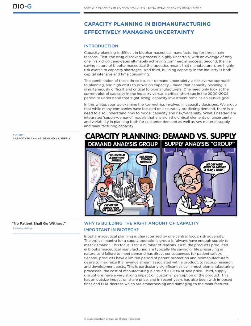
In this whitepaper we examine the key metrics involved in capacity decisions. We argue that while many companies have focused on accurately predicting demand, there is a need to also understand how to model capacity and risk/variability. What’s needed are integrated ‘supply-demand’ models that envision the critical elements of uncertainty and variability in planning both for customer demand as well as raw material supply and manufacturing capacity.

WHY IS BUILDING THE RIGHT AMOUNT OF CAPACITY IMPORTANT IN BIOTECH?Biopharmaceutical planning is characterized by one central focus: risk adversity. The typical mantra for a supply operations group is “always have enough supply to meet demand”. This focus is for a number of reasons. First, the products produced in biopharmaceutical manufacturing are typically life saving or life preserving in nature, and failure to meet demand has direct consequences for patient safety. Second, products have a limited period of patent protection and biomanufacturers desire to maximize the revenue stream associated with a product, to recoup research and development costs. This is particularly significant since in most biomanufacturing processes, the cost of manufacturing is around 10-20% of sale price. Third, supply disruptions have a very strong impact on customer perception of the product. This has an outsize impact on share price, and in recent years has also been with imposed fines and FDA decrees which are embarrassing and damaging to the manufacturer.

FIGURE 1: CAPACITY PLANNING: DEMAND VS. SUPPLY

CAPACITY PLANNING IN BIOMANUFACTURING EFFECTIVELY MANAGING UNCERTAINTY

“No Patient Shall Go Without” Industry Adage

2© Bioproduction Group. All Rights Reserved.


These factors mean that capacity planning in biomanufacturing is seldom interested in ‘average’, or expected performance. Risk adversity requires that sufficient capacity is made at a much higher service level (say, the 75%ile, or 95%ile). However, this raises significant modeling challenges for biopharmaceutical organizations. If planning over a long horizon (say, 5-10 years), and for very high service levels with significant uncertainty in demand and variability in supply, it is likely that we will build too much capacity. Such high service levels are also very sensitive to inflated estimates of either supply capability or demand requirements: relatively small errors have cumulatively large effects when planning to a high service level. However, through a better understanding of both existing capacity and potential future demand, it is possible to build strategies that will limit over-investment while ensuring better tolerance to risk and variability.

BUILDING ACCURATE MODELS OF DEMANDThere are many complexities to creating accurate models of demand that are outside the scope of this white paper. In this paper we will focus on the key elements of variability that impact supply: the likelihood that a product will launch, and the demand for the product and variability if it does launch. Probability of Technical Success (PTS) is the common standard used by the industry to describe the likelihood that a product will be commercially successful. For example, if we have 6 products in our pipeline and each one has a PTS of 20%, then we assume that the ‘expected’ number of products that will launch will be 6x0.2 = 1.2 products.

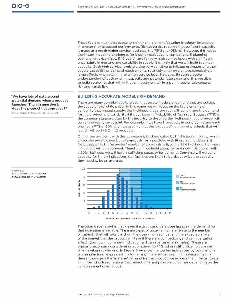
One of the problems with this approach is best indicated by the histogram below, which shows the possible number of approvals for a portfolio with 16 drug candidates in it. Note that, while the ‘expected’ number of approvals is 6, with a 25% likelihood 8 or more indications will be approved. Therefore, if we build capacity for 6 new indications, with a 50% likelihood we will have insufficient capacity for demand. Conversely, if we build capacity for 11 new indications, our facilities are likely to be about twice the capacity they need to be on average.

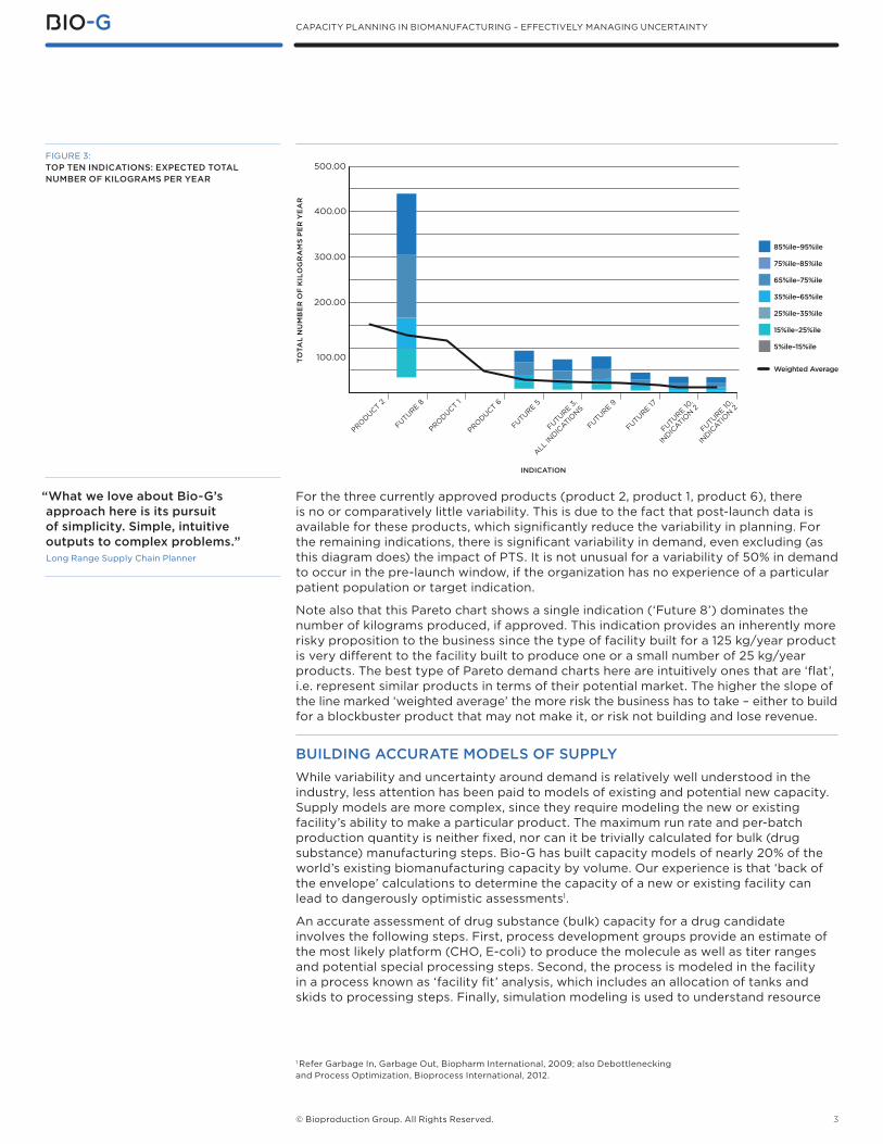
The other issue raised is that – even if a drug candidate does launch – the demand for that indication is variable. The main types of uncertainty here relate to the number of patients that will take the drug, the dosing for each patient, the expected share of the market that the product will take if there are competitors, and cannibalization effects (i.e. how much a new indication will cannibalize existing sales). These are typically secondary considerations compared to PTS but are still critical to consider when evaluating demand. In Figure 3 we show the top ten indications by volume for a biomanufacturer, expressed in kilograms of material per year. In this diagram, rather than showing just the ‘average’ demand for the product, we express the uncertainties in a number of colored regions that reflect different possible outcomes depending on the variables mentioned above.

“We have lots of data around potential demand when a product launches. The big question is, does the product get approved?” Senior Capacity Planner, Top-10 Biotech

NUMBER OF COMMERCIAL SUCCESSES, 2011-2015

0 1 2 3 4 5 6 7 8 9 10 11 12 13 14 15 16 17

4

12

16

20

8

LIK

ELI

HO

OD

(%

)

50% > 6 INDICATIONS

25% > 8 INDICATIONS

5% ≥ 11 INDICATIONS

FIGURE 2: HISTOGRAM OF NUMBER OF SUCCESSES BY INDICATION



For the three currently approved products (product 2, product 1, product 6), there is no or comparatively little variability. This is due to the fact that post-launch data is available for these products, which significantly reduce the variability in planning. For the remaining indications, there is significant variability in demand, even excluding (as this diagram does) the impact of PTS. It is not unusual for a variability of 50% in demand to occur in the pre-launch window, if the organization has no experience of a particular patient population or target indication.

Note also that this Pareto chart shows a single indication (‘Future 8’) dominates the number of kilograms produced, if approved. This indication provides an inherently more risky proposition to the business since the type of facility built for a 125 kg/year product is very different to the facility built to produce one or a small number of 25 kg/year products. The best type of Pareto demand charts here are intuitively ones that are ‘flat’, i.e. represent similar products in terms of their potential market. The higher the slope of the line marked ‘weighted average’ the more risk the business has to take – either to build for a blockbuster product that may not make it, or risk not building and lose revenue.

BUILDING ACCURATE MODELS OF SUPPLYWhile variability and uncertainty around demand is relatively well understood in the industry, less attention has been paid to models of existing and potential new capacity. Supply models are more complex, since they require modeling the new or existing facility’s ability to make a particular product. The maximum run rate and per-batch production quantity is neither fixed, nor can it be trivially calculated for bulk (drug substance) manufacturing steps. Bio-G has built capacity models of nearly 20% of the world’s existing biomanufacturing capacity by volume. Our experience is that ‘back of the envelope’ calculations to determine the capacity of a new or existing facility can lead to dangerously optimistic assessments1.

An accurate assessment of drug substance (bulk) capacity for a drug candidate involves the following steps. First, process development groups provide an estimate of the most likely platform (CHO, E-coli) to produce the molecule as well as titer ranges and potential special processing steps. Second, the process is modeled in the facility in a process known as ‘facility fit’ analysis, which includes an allocation of tanks and skids to processing steps. Finally, simulation modeling is used to understand resource

“What we love about Bio-G’s approach here is its pursuit of simplicity. Simple, intuitive outputs to complex problems.” Long Range Supply Chain Planner

FIGURE 3: TOP TEN INDICATIONS: EXPECTED TOTAL NUMBER OF KILOGRAMS PER YEAR

INDICATION

PRODUCT 2

FUTURE 8

PRODUCT 1

PRODUCT 6

FUTURE 5

FUTURE 3,

ALL IN

DICATIO

NS

FUTURE 9

FUTURE 17

FUTURE 10,

INDIC

ATION 2

FUTURE 10,

INDIC

ATION 2

100.00

200.00

300.00

400.00

500.00

TO

TAL

NU

MB

ER

OF

KIL

OG

RA

MS

PE

R Y

EA

R

85%ile–95%ile

75%ile–85%ile

65%ile–75%ile

35%ile–65%ile

25%ile–35%ile

15%ile–25%ile

5%ile–15%ile

Weighted Average

1 Refer Garbage In, Garbage Out, Biopharm International, 2009; also Debottlenecking and Process Optimization, Bioprocess International, 2012.



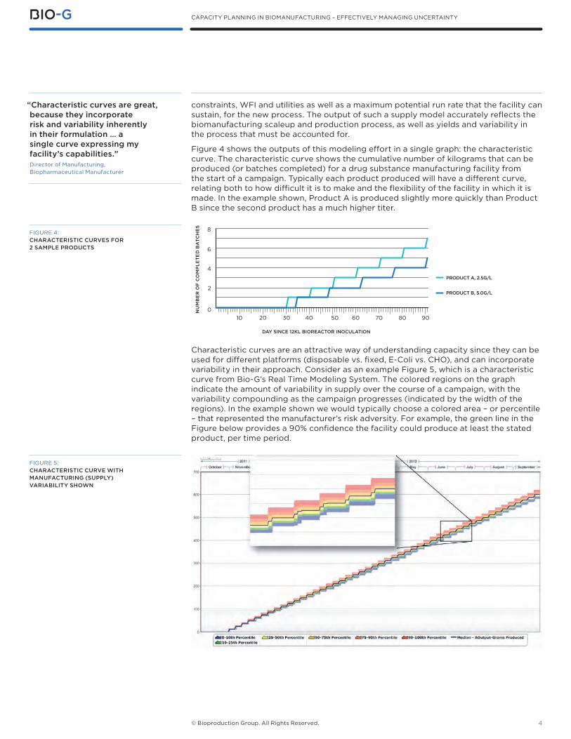
constraints, WFI and utilities as well as a maximum potential run rate that the facility can sustain, for the new process. The output of such a supply model accurately reflects the biomanufacturing scaleup and production process, as well as yields and variability in the process that must be accounted for.

Figure 4 shows the outputs of this modeling effort in a single graph: the characteristic curve. The characteristic curve shows the cumulative number of kilograms that can be produced (or batches completed) for a drug substance manufacturing facility from the start of a campaign. Typically each product produced will have a different curve, relating both to how difficult it is to make and the flexibility of the facility in which it is made. In the example shown, Product A is produced slightly more quickly than Product B since the second product has a much higher titer.

Characteristic curves are an attractive way of understanding capacity since they can be used for different platforms (disposable vs. fixed, E-Coli vs. CHO), and can incorporate variability in their approach. Consider as an example Figure 5, which is a characteristic curve from Bio-G’s Real Time Modeling System. The colored regions on the graph indicate the amount of variability in supply over the course of a campaign, with the variability compounding as the campaign progresses (indicated by the width of the regions). In the example shown we would typically choose a colored area – or percentile – that represented the manufacturer’s risk adversity. For example, the green line in the Figure below provides a 90% confidence the facility could produce at least the stated product, per time period.

“Characteristic curves are great, because they incorporate risk and variability inherently in their formulation … a single curve expressing my facility’s capabilities.” Director of Manufacturing, Biopharmaceutical Manufacturer

FIGURE 4: CHARACTERISTIC CURVES FOR 2 SAMPLE PRODUCTS

FIGURE 5: CHARACTERISTIC CURVE WITH MANUFACTURING (SUPPLY) VARIABILITY SHOWN

DAY SINCE 12KL BIOREACTOR INOCULATION

010 20 30 40 80706050 90

2

6

8

4

NU

MB

ER

OF

CO

MP

LET

ED

BA

TC

HE

S

PRODUCT A, 2.5G/L

PRODUCT B, 5.0G/L



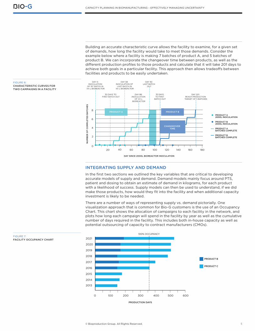
Building an accurate characteristic curve allows the facility to examine, for a given set of demands, how long the facility would take to meet those demands. Consider the example below where a facility is making 7 batches of product A, and 5 batches of product B. We can incorporate the changeover time between products, as well as the different production profiles to those products and calculate that it will take 201 days to achieve both goals in a particular facility. This approach then allows tradeoffs between facilities and products to be easily undertaken.

INTEGRATING SUPPLY AND DEMAND In the first two sections we outlined the key variables that are critical to developing accurate models of supply and demand. Demand models mainly focus around PTS, patient and dosing to obtain an estimate of demand in kilograms, for each product with a likelihood of success. Supply models can then be used to understand, if we did make those products, how would they fit into the facility and when additional capacity investment is likely to be needed.

There are a number of ways of representing supply vs. demand pictorially. One visualization approach that is common for Bio-G customers is the use of an Occupancy Chart. This chart shows the allocation of campaigns to each facility in the network, and plots how long each campaign will spend in the facility by year as well as the cumulative number of days required in the facility. This includes both in-house capacity as well as potential outsourcing of capacity to contract manufacturers (CMOs).

FIGURE 6: CHARACTERISTIC CURVES FOR TWO CAMPAIGNS IN A FACILITY

FIGURE 7: FACILITY OCCUPANCY CHART

DAY SINCE 2000L BIOREACTOR INOCULATION

020 40 60 80 160

DAY 0: INOCULATION

OF 1ST BATCH IN XX L BIOREACTOR

30 DAYS TO FIRST BATCH OUT

DAY 58: INOCULATION OF

LAST BATCH IN XX L BIOREACTOR

DAY 88: INOCULATION

OF XX L BIOREACTOR

35 DAYS TO FIRST

BATCH OUT

DAY 201: REACH PRODUCTION

TARGET OF 5 BATCHES

DAY 92: LAST BATCH

OUT

140120100 180

2

6

8

4

NU

MB

ER

OF

CO

MP

LET

ED

BA

TC

HE

S

PRODUCT B

PRODUCT ABATCHES COMPLETE

PRODUCT BBATCHES COMPLETE

PRODUCT B2000L INOCULATION

PRODUCT A2000L INOCULATION

PRODUCT A

CHANGEOVER TIME

PRODUCTION DAYS

1000 200 300 400 500 600

2013

2017

2019

2021

2015

2016

2018

2020

2014

PRODUCT B

100% OCCUPANCY

PRODUCT C



In the Facility Occupancy chart shown above, characteristic curves are used to convert yearly demand requirements in kilograms, to the number of production days in a facility at a particular service level (say, the 95%ile). The output is a chart showing, for each year, the number of days that will be spent making each of the products allocated to that facility. Management can then quickly establish both the relative impact of each product in the facility using in a common metric, as well as the year when production facilities will no longer be sufficient. In the example shown, the facility will run out of capacity in 2017, but with a 10% improvement in efficiency will be able to stretch out capacity till 2018. This approach then allows tradeoffs between facilities and products to be easily undertaken.

EVALUATING THE IMPACT OF TITER One of the most significant elements of variability when considering new capacity in biopharmaceutical operations is the titer of new products. Titer is a measure of the productivity of the fermentation process. In the past 20 years, titer has doubled every 2 years or so, effectively doubling the amount of material produced by each batch. However purification technologies have not increased efficiency at the same rate, moving the bottleneck (or rate-limiting steps) to downstream.

Titer is especially important to consider in bulk biopharmaceutical supply since most facilities are designed for titers that are lower than the products they will eventually produce. For example, most facilities designed in the 2000-2005 period were designed at a titer of around 1 gram per liter. Processing materials of 2 or more grams per liter places stresses on downstream buffer preparation and hold vessels, as well as column capacities and in some cases product hold vessels between process steps. This in turn slows down the processing of these steps, with facility staff forced to re-batch material, or re-use tanks.

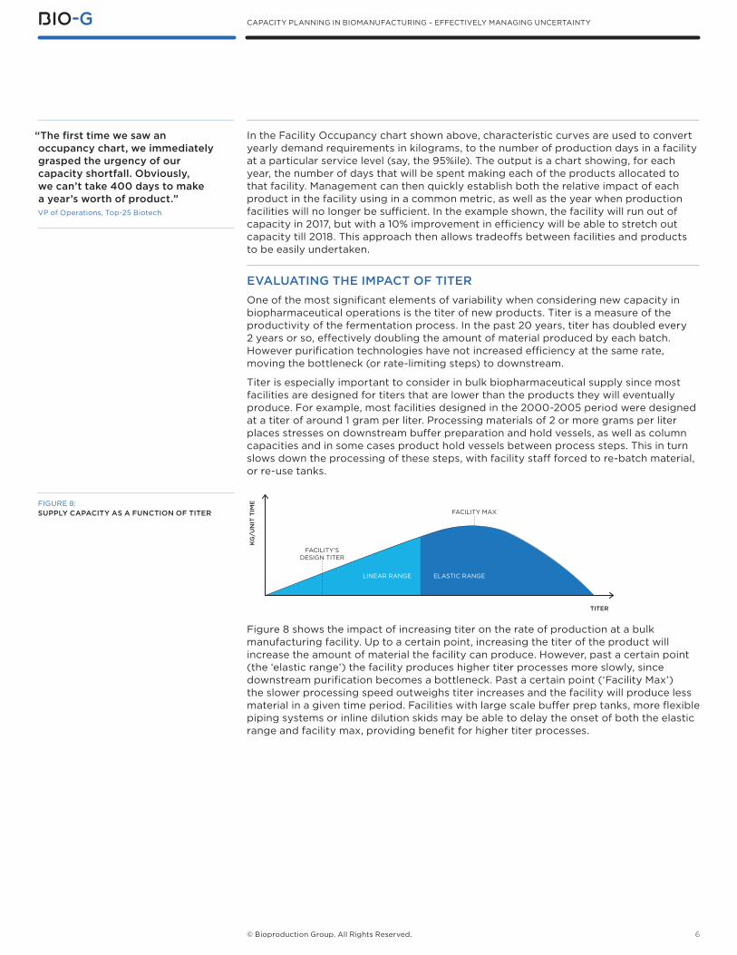
Figure 8 shows the impact of increasing titer on the rate of production at a bulk manufacturing facility. Up to a certain point, increasing the titer of the product will increase the amount of material the facility can produce. However, past a certain point (the ‘elastic range’) the facility produces higher titer processes more slowly, since downstream purification becomes a bottleneck. Past a certain point (‘Facility Max’) the slower processing speed outweighs titer increases and the facility will produce less material in a given time period. Facilities with large scale buffer prep tanks, more flexible piping systems or inline dilution skids may be able to delay the onset of both the elastic range and facility max, providing benefit for higher titer processes.

FIGURE 8: SUPPLY CAPACITY AS A FUNCTION OF TITER

KG

/UN

IT T

IME

TITER

FACILITY’SDESIGN TITER

LINEAR RANGE ELASTIC RANGE

FACILITY MAX

“The first time we saw an occupancy chart, we immediately grasped the urgency of our capacity shortfall. Obviously, we can’t take 400 days to make a year’s worth of product.” VP of Operations, Top-25 Biotech



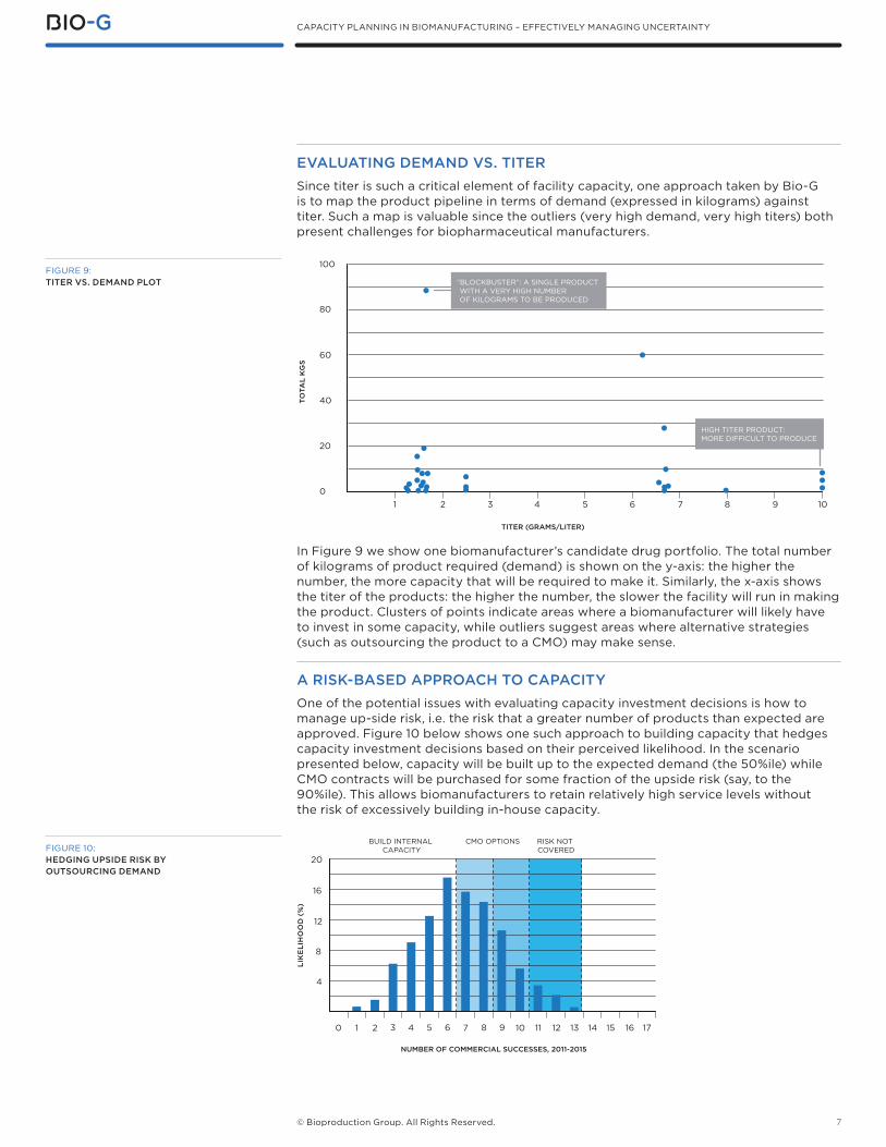
EVALUATING DEMAND VS. TITERSince titer is such a critical element of facility capacity, one approach taken by Bio-G is to map the product pipeline in terms of demand (expressed in kilograms) against titer. Such a map is valuable since the outliers (very high demand, very high titers) both present challenges for biopharmaceutical manufacturers.

In Figure 9 we show one biomanufacturer’s candidate drug portfolio. The total number of kilograms of product required (demand) is shown on the y-axis: the higher the number, the more capacity that will be required to make it. Similarly, the x-axis shows the titer of the products: the higher the number, the slower the facility will run in making the product. Clusters of points indicate areas where a biomanufacturer will likely have to invest in some capacity, while outliers suggest areas where alternative strategies (such as outsourcing the product to a CMO) may make sense.

A RISK-BASED APPROACH TO CAPACITYOne of the potential issues with evaluating capacity investment decisions is how to manage up-side risk, i.e. the risk that a greater number of products than expected are approved. Figure 10 below shows one such approach to building capacity that hedges capacity investment decisions based on their perceived likelihood. In the scenario presented below, capacity will be built up to the expected demand (the 50%ile) while CMO contracts will be purchased for some fraction of the upside risk (say, to the 90%ile). This allows biomanufacturers to retain relatively high service levels without the risk of excessively building in-house capacity.

FIGURE 9: TITER VS. DEMAND PLOT

FIGURE 10: HEDGING UPSIDE RISK BY OUTSOURCING DEMAND

NUMBER OF COMMERCIAL SUCCESSES, 2011-2015

CMO OPTIONS RISK NOT COVERED

BUILD INTERNAL CAPACITY

0 1 2 3 4 5 6 7 8 9 10 11 12 13 14 15 16 17

4

12

16

20

8

LIK

ELI

HO

OD

(%

)

TITER (GRAMS/LITER)

40

60

80

100

20

01 2 3 4 5 6 7 8 9 10

TO

TAL

KG

S

HIGH TITER PRODUCT:MORE DIFFICULT TO PRODUCE

“BLOCKBUSTER”: A SINGLE PRODUCT WITH A VERY HIGH NUMBER OF KILOGRAMS TO BE PRODUCED



FEEDBACK Please provide your feedback at http://www.zoomerang.com/Survey/WEB22AYVM3VLFC

FURTHER READINGJohnston, Zhang (2009). Garbage In, Garbage Out: The Case for More Accurate Process Modeling in Manufacturing Economics, Biopharm International, 22:8

MORE INFORMATION

BIOPRODUCTION GROUP [email protected] WWW.BIO-G.COM

The hedging strategies that have been most successful in the industry are those that allow biomanufacturers to delay investment in capacity until 2 years before that capacity is needed. For example, a contract with a CMO may purchase a certain number of days in a facility, with the option to cancel 2 years before production starts at only 50% of the cost. Since most of the uncertainty in a portfolio is resolved within the 2 year planning horizon, such an approach limits risk – even if using the CMO is more expensive than building internal capacity. Other alternatives, like building a ‘greenfields’ facility, involve investment of significant capital 4-5 years before capacity is needed. This commits the biomanufacturer to building capacity well before the uncertainties in both demand and supply are resolved. As such, deferral of capacity investment is one of the most important aspects of provisioning capacity in biomanufacturing.

PLANNING FOR RELIABLE SUPPLY Biomanufacturers today are faced with a difficult planning problem: when to invest in capacity to ensure high service levels while minimizing capital outlay. The problem is unique to the biopharmaceutical community since today’s facilities are relatively inflexible to variables like titer and number of products produced. Plus, capital costs are high. A risk-based approach to planning like the one outlined here has a number of benefits for a biomanufacturer: 1. It focuses planning effort on the small number of variables that are important. While the traditional focus has been around PTS we believe a more holistic approach is required that examines more thoroughly both demand and supply variability and risk. 2. It minimizes the ‘regret’ associated with investing in capacity and then discovering it is not needed. Deferring capital expenditure until risk is better understood may result in a more expensive per-kilogram cost if a product is approved, but minimizes the likelihood that a company will make significant investments in capacity that is not needed.

Such an approach can also be implemented successfully without use of highly complex algebra or statistics, and can be visualized in outputs like characteristic curves and occupancy charts. Such integrated supply-demand capacity models can provide increased visibility for the business. They also reduce capital spending, while aligning manufacturing and process development groups to ensure that demand can be met reliably at the lowest cost.

“Risk based approaches are critical when evaluating capacity. If you don’t consider up-side risk, you’re leaving money on the table.”Finance Director, Biopharmaceutical Manufacturer

capacity planning in biomanufacturing

Documents