capacity, entry deterrence, and … · other hand, acts as a stackelberg leader in output. if entry...

_ xi4,;‘:

CAPACITY, ENTRY DETERRENCE, AND HORIZONTAL MERGER

bv

Kyung Hwan Baik

Dissertation submitted to the Faculty of the

Virginia Polytechnic Institute and State University

in partial fulfillment of the requirements for the degree of

DOCTOR OF PHILOSOPHY

in

Economics

APPROVED:

” ‘Lt

Jac s Cremer, Chairman . Amo Kats, Chairman

Y Y° ,ß· / 01 W/bi

Herve Moulin

,/Z

//CatherineEckel /Hans Haller

May, 1989

Blacksburg, Virginia

Q .

$¤ „

tCAPACITY, ENTRY DETERRENCE, AND HORIZONTAL MERGER

l

i byQ

Kyung I-Iwan Baik

\¢ Committee Chairmen: Jacques Cremer and Amoz KatsÄ}: Economics

(ABSTRACT)

This dissertation examines the free rider problem of entry deterrence,

the profitability of a horizontal merger, and the effects of a horizontal

merger on the outsiders’ profits and industry prices, in the markets where

firms' capacity costs are sunk.

We investigate the free rider problem of entry deterrence in the

subgame perfect Nash equilibria of a three—stage game in which in the first

stage multiple incumbent firms choose their capacities simultaneously and

independently, in the second stage a potential entrant, after observing the

incumbent firms’ capacity vector, chooses its capacity, and in the third stage

the firms engage in capacity·constrained Cournot competition. We show that

the free rider problem may occur: there are situations where both entry

prevention and allowing entry are equilibria but entry prevention is Pareto

superior for the incumbent firms. We also show that increasing the number of

incumbent firms may cause the equilibrium price to increase and thus

consumer welfare to decrease. The free rider problem is still manifested in a

modified model in which multiple potential entrants choose their capacities

sequentially after the first stage incumbents’ capacity decisions.

Several recent papers which theoretically analyze the profitability of a

horizontal merger and its effects on the outsiders’ profits and industry prices,

all observe that a merger never decreases industry prices, a merger to a

monopoly is always profitable, and a merger never hurts the outsiders.

However, we demonstrate, in a market for a homogeneous product where

firms with sunk capacities compete in quantities and there are potential

entrants, that a merger can decrease industry price and a merger of incumbent

firms to a monopoly may not be profitable. We also show, in a market for a

homogeneous product where firms with sunk capacities engage in capacity-

constrained price competition, that a merger can hurt the outsiders.

To My Parents

ACKNOWLEDGEMENTS

v

TABLE OF CONTENTS

CHAPTER I INTRODUCTION ..............................1

1. Strategic Entry Deterrence and Sunk Capacity Costs .............1

2. Entry Deterrence and the Free Rider Problem ................. 3

3. Horizontal Mergers and Three Common Observations .............7

CHAPTER II CAPACITY, ENTRY DETERRENCE, AND

THE FREE RIDER PROBLEM ..............................9

1. Introduction .......................................9

2. The Model .......................................13

3. Capacity-Constrained Subgames .......................... 16

4. Subgame Perfect Equilibria of the Full Game ................. 22

5. Possible Underinvestment in Entry Deterrence ................ 40

6. Comparative Statics .................................44

7. The Case of Multiple Potential Entrants ....................52

8. Conclusions ...................................... 56

CHAPTER III SUNK CAPACITY COSTS, HORIZONTAL MERGER,

AND INDUSTRY PRICE ................................. 60

1. Introduction ......................................60

2. The Model .......................................63

3. A Price-Decreasing Merger .............................65

vi

4. An Entry-Inducing Merger to Monopoly .....................70

5. Conclusions ...................................... 74

CHAPTER IV SUNK CAPACITY COSTS AND HORIZONTAL MERGER

WITH CAPACITY-CONSTRAINED BERTRAND COMPETITION .........77

1. Introduction ......................................77

2. The Model .......................................79

3. Duopoly with Capacity-Constrained Price Competition ............82

4. An Outsider-Hurting Merger ............................89

5. Conclusions ...................................... 93

CHAPTER V SUMMARY AND CONCLUSIONS ...................96

BIBLIOGRAPHY ......................................100

APPENDICES .......................................104

Appendix A ........................................ 105

Appendix B ........................................ 112

Appendix C ........................................ 114

VITAE ...........................................116

vii

LIST OF FIGURES

FIGURE 2.1. Firm2’s

Subgame Perfect Reaction Correspondence and

Nonexistence of Equilibrium .....................25


Subgame Perfect Reaction Correspondence .......37

FIGURE 2.3. A Continuum of Entry-Allowing Equilibria ............ 39

FIGURE 2.4. Subgame Perfect Equilibria in (F, ot) Space with m = 1 .... 47

FIGURE 2.5. Subgame Perfect Symmetric Equilibria in (F, on) Space

with m - 2 ................................48

FIGURE 2.6. A Decrease in the Total Equilibrium Output When

m Increases from One to Two .................... 50

FIGURE 3.1. The Equilibrium Outputs with the Initial

Capacity Vector ............................ 67


Postmerger Capacity .................... 69

FIGURE 4.1. The Equilibrium of the (kl, kg) Subgame ............. 83


Subgame Perfect Reaction Correspondence .......87

FIGURE 4.3. Increases in Capacity Levels after the Merger ..........90

viii

CHAPTER I

INTRODUCTION

1. STRATEGIC ENTRY DETERRENCE AND SUNK CAPACITY COSTS

Consider a market situation in which there are a single established firm

(or a coordinated cartel), called the incumbent, and a single potential entrant.

There are two periods: preentry and postentry. The market demand is

constant through the periods. In the preentry period, the incumbent chooses

and produces at an output level which it will maintain in the postentry

period. At the beginning of the postentry period, taking the incumbent’s

output level as given, the potential entrant decides whether or not to enter

and if so how much to produce. It enters if and only if it can make a positive

profit. After the decisions of the potential entrant are made, the active

firm(s) in the market produce(s) at the predetermined output level(s). Their

products are homogeneous and consumers can switch firms without any costs.

These are all essential assumptions of the classic model of strategic

entry deterrence, called the Bain-Sylos-Modigliani (BSM) limit pricing model.

The potential entrant in the model believes that the incumbent will produce, in

the postentry period, at the output level committed in the preentry period

regardless of the potential entrant’s decisions (the Bain-Sylos postulate).

Thus if the entrant enters, it becomes a Cournot follower and chooses a

Cournot best response to the incumbent’s output. The incumbent, on the

l

2

other hand, acts as a Stackelberg leader in output. If entry deterrence is

profitable when compared with accommodation, the incumbent commits to the

“limit output" and prevents the potential entrant from entering the market.

Otherwise, it allows the entrant to enter.

However, the assumption that the incumbent can convince the potential

entrant that it will maintain the same output in the postentry period as its

preentry output regardless of whether or not entry occurs, is dubious. The

incumbent’s optimal response to entry is usually an accommodating output

reduction and given the entrant’s knowledge of the fact, the entrant treats the

incumbent’s threat that it will continue to produce at the committed output as

empty and thus enters the market.

Recognizing that the incumbent’s prior (to the entrant’s decisions) and

irreversiblc investment in entry deterrence can be a credible threat

(equivalent to commitment), Spence (1977) proposed a model in which the

incumbent installs capacity in the preentry period and capacity costs are

Stmk. The potential entrant believes, in that model, that if it enters the

incumbent’s output will be equal to its installed capacity. Thus, entry preven-

tion is always feasible like in the BSM limit pricing model and excess capacity

may be observed even in the case of a linear demand.

However, the incumbent’s threat that it will produce up to its capacity

if the entrant enters, can be empty. For example, in the two-stage model of

Dixit (1980), if the incumbent’s installed capacity is greater than its output at

the intersection of its variable-cost Cournot reaction function and the

entrant’s ful1—cost reaction function, then the incumbent’s optimal response to

entry is to choose the output at the intersection.

3

Dixit (1980) studies a perfect equilibrium in a model which is basically

the same as Spence’s and shows that in the case where each firm’s marginal

revenue is always decreasing in the other’s output, excess capacity is never

observed in a perfect equilibrium. There are situations where preventing

entry is profitable in Spence’s model but not feasible in Dixit’s (1980).

Dixit (1980) assumes that in the second stage while the incumbent’s

capacity costs are sunk, those of the entrant are variable. Ware (1984) argues

that if the incumbent’s capacity costs are sunk, then those of the entrant are

equally so and must also be committed before production takes place. He thus

proposes a three-stage model in which the incumbent and the entrant

sequentially choose their capacities and then engage in capacity-constrained

Cournot competition. The incumbent has a harder time preventing entry than

suggested by Dixit (1980) but it still maintains a strategic advantage over the

entrant because it sinks capacity before the entrant does.

In Chapters II, III, and IV of this dissertation, we consider market

situations where firms have sunk capacity costs, and develop our arguments

based on three-stage models, following Ware’s proposal.

2. ENTRY DETERRENCE AND THE FREE RIDER PROBLEM

Beginning with the seminal work of Bain (1956), the early literature on

strategic entry deterrence has concentrated on a market situation in which a

single incumbent firm (or group of colluding incumbents) confronts a single

potential entrant. This includes, for example, Spence (1977), Salop (1979),

4

Dixit (1979), (1980), Spulber (1981), Schmalensee (1981), Kreps and Wilson (1982),

Milgrom and Roberts (1982), Fudenberg and Tirole (1983), Ware (1984), Bulow,

Geanakoplos, and Klemperer (1985), and Allen (1986). In these works, the

incumbent prevents the potential entrant from entering the market if entry

deterrence is feasible and also profitable when compared with accommodation.

Recently, the literature has been dominated by market situations in

which an established oligopoly of competing firms faces a potential entrant (or

multiple entrants), and in which all noncooperative firms enter the market

sequentially. For example, Prescott and Visscher (1977), pioneering the ideas

of sequential entry and endogenous market structure, analyze a model in which

firms with perfect foresight about subsequent entry and location decisions

enter the market and choose locations sequentially. Bernheim (1984) develops

a model of sequential entry into an industry and demonstrates that standard

government policies may have the perverse effect of increasing industrial

concentration. I-le also investigates the ability of a noncooperative oligopoly

to prevent entry when member firms simultaneously commit to deterrence

investments. Gilbert and Vives (1986) consider a market where several

incumbents facing a potential entrant choose simultaneously and independently

postentry output levels. Harrington (1987) examines the effect on entry

deterrence of asymmetric information about the constant marginal cost between

a noncooperative oligopoly and potential entrants. Vives (1988) analyzes a

model with quantity commitments where an incumbent (or several incumbents)

faces a sequence of potential entrants. Eaton and Ware (1987) study

noncooperative entry deterrence in a sequential entry model where firms sink

capacity costs at the time of entry and market structure is determined

« S

endogenously, and McLean and Riordan (1989) do so in a sequential entry model

where upon entering, each firm irreversibly chooses a type of technology and

market structure is determined endogenously.

Entry deterrence in the models characterized by multiple incumbents has

the properties of a public good. lf some firms prevent entry, all firms in the

industry are protected from the new competitors. That is, "consumption” of

entry deterrence is not exclusive. Also, one firm’s consumption of entry

deterrence does not reduce its amount enjoyed by other firms. Since firms in

the above—mentioned studies cannot collude on investments in entry deterrence,

each firm may free-ride on its rivals’ provision of the public good and the

free rider problem suggests that there would be underinvestment in entry

deterrence.

The seminal work which discusses the free rider problem of entry

deterrence is Bernheim’s. In his model there are cases where both entry

prevention and allowing entry are equilibria, but entry prevention is mutually

more profitable than allowing entry. Thus one may say that there may be

underinvestment in entry deterrence. He argues, however, that there is no

such phenomenon because whenever entry prevention is jointly profitable

when compared to allowing entry, sufficient deterrence investment is normally

expected to be undertaken even by a noncooperative oligopoly. He actually

applies to the model the solution concept of a coalition-proof Nash equilibrium

introduced in Bernheim, Peleg, and Whinston (1987). Gilbert and Vives

demonstrates that the free rider problem never occurs in their model.

Waldman (1987a) shows that in the model of Gilbert and Vives there is no

evidence of underinvestment in entry deterrence even if the incumbent firms

6

are uncertain about the exact investment in entry deterrence needed to deter

entry. He shows, on the other hand, that in Bernheim’s model there is a

strong tendency to underinvest in entry deterrence if incumbent firms are

uncertain about the exact investment in entry deterrence needed to deter

entry. Harrington finds the same situations as Berheim and states that

potentially the free rider problem of entry deterrence does exist. Eaton and

Ware never find underinvestment in entry deterrence in the sense that the

number of firms in the equilibrium is the smallest that can deter entry.

McLean and Riordan observe that the free rider problem frequently occurs.

Waldman (1987b) points out that in the model of McLean and Riordan the free

rider problem arises even if a group of early entrants (or incumbent firms) are

assumed to move simultaneously. He also argues there that the free rider

problem matters if some factor is present which smooths the return to

investing in entry deterrence.

Gilbert and Vives examine the free rider problem of entry deterrence inn

a two-stage model where multiple incumbent firms facing a single potential

entrant commit noncooperatively to postentry output levels and then the

entrant’s decisions follow. In Chapter II of the dissertation, we show that

their observation of nonexistence of the free rider problem totally relies on

the Bain—Sylos postulate which they assume. Indeed, introducing sunk

capacity costs which are typically considered as credible entry deterrence

investment and adopting a three-stage game ä la Ware (1984), we demonstrate

that the free rider probem can occur. We illustrate that there are situations

where both entry prevention and allowing entry are subgame perfect equilibria

but entry prevention is mutually more profitable than allowing entry. The

7

reason why our observation differs from that of Gilbert and Vives is that

entry prevention is not always feasible in our model while it is in theirs.

3. HORIZONTAL MERGERS AND THREE COMMON OBSERVATIONS

Defining a horizontal merger as a union of independent firms in the same

market into a single entity under the control of a single decision maker,

several recent papers theoretically analyze its profitability and its effects on

the outsiders’ profits and industry prices.

Are mergers beneficial to the merging parties (insiders)? The answers to

the question differ across the studies. Szidarovszky and Yakowitz (1982),

Salant, Switzer, and Reynolds (1983), Davidson and Deneckere (1984), and Perry

and Porter (1985) all demonstrate that mergers may reduce the joint profits of

the constituent firms (insiders) in quantity-setting games. Davidson and

Deneckere (1984) and Deneckere and Davidson (1985) show that mergers are

never disadvantageous in static price—setting games.

The above-mentioned studies, on the other hand, coincide in the

following observations: (i) a merger, profitable or not, never decreases

industry prices, (ii) a merger to a monopoly is always profitable, and (iii) a

merger never hurts the outsiders.

However, drawing on the models prevalent in the industrial organization

literature, we illustrate in Chapters III and IV of the dissertation that the

three common observations can be reversed. In particular, Chapter III

provides both an example in which a merger causes industry price to decrease,

8

and an example in which a merger to a monopoly is not profitable. Chapter IV

provides an example in which a merger hurts outsiders.

We consider, in Chapter III, a market for a homogeneous product where

firms with sunk capacities compete in quantities and there are potential

entrants, and in Chapter IV, a market for a homogeneous product where firms

with sunk capacities engage in capacity-constrained price competition. In both

markets firms cannot decrease their capacities since their capacity costs are

sunk. Our arguments are made in the context of three-stage games. We treat

each merged entity as a single firm with the combined capacity of insiders and

then give it a strategic advantage that it can decide whether or not to

increase its capacity before outsiders do. The latter assumption, which is not

innocuous for the result in Chapter IV, seems to be natural because the

merged firm can commit to its postmerger capacity before it announces the

merger. '

CHAPTER ll

CAPACITY, ENTRY DETERRENCE, ANDTHE FREE RIDER PROBLEM

1. INTRODUCTION

Since the seminal work of Bain (1956), the literature on strategic entry

deterrence has grown rapidly. The early works in this area restricted

attention to a market situation in which a single incumbent firm (or a

coordinated cartel) faces a single potential entrant. Works by Spence (1977),

Salop (1979), Dixit (1979), (1980), Spulber (1981), Schmalensee (1981), Fudenberg

and Tirole (1983), and Ware (1984) are examples. Recently, attention has

moved from the one incumbent one entrant framework to models in which

multiple competing incumbent firms confront a single potential entrant ( e.g.,

Gilbert and Vives (1986), Harrington (1987), and Waldman (1987a), (1987b) ) and

to models in which firms sequentially enter an industry ( e.g., Prescott and

Visscher (1977), Bernheim (1984), Eaton and Ware (1987), and McLean and

Riordan (1989) ). These works focus on the free rider problem of entry deter-

rence and/or the effects of sequential entry on elements of market structure.

Entry deterrence in them has the characteristics of a public good. lf some

firms prevent entry, all firms in the industry are protected from the new

competitors. Since firms in these models cannot collude on investment in

entry deterrence, examining the free rider problem of entry deterrence should

9

10

be an interesting issue.

Gilbert and Vives examine the free rider problem of entry deterrence in

a two-stage model in which in the first stage multiple incumbent firms facing a

potential entrant which must pay a fixed cost to enter the industry, decide

independently how much to produce and in the second stage the potential

entrant decides whether to enter or not, and if it enters how much to produce.

They conclude that in their model the free rider problem never occurs: there

is no underinvestment in entry deterrence.1 Waldman (1987a) shows that in

the model of Gilbert and Vives even if the incumbent firms are uncertain

about the cost of entry and thus uncertain about the exact investment in

entry deterrence needed to deter entry, there is no evidence of an

underinvestment in entry deterrence.2

However, the result of Gilbert and Vives critically relies on the assump-

tion that the incumbent firms are able to convince the potential entrant that

they will produce at their committed output levels regardless of the potential

entrant’s actions. Indeed, their model is an extension of the Bain-Sylos—

Modigliani limit pricing model to the case of multiple incumbent firms.3 Notice

that in the recent literature on strategic entry deterrence, output has beenU

typically regarded as a noncredible entry deterrence instrument.

We introduce the installation of capacity as a sunk investment in entry

deterrence, which has been considered a credible entry deterrent in this area

(e.g., Spence (1977), Dixit (1979), (1980), Schmalensee (1981), Spulber (1981),

Ware (1984)). In particular we adopt the proposal in Ware (1984) that as long

as the instrument of strategic commitment takes the form of sunk costs, which

both a potential entrant and an incumbent firm must incur, a three—stage model

11

is required. Since a potential entrant in our model must also install capacity

(sink capacity costs) before production takes place, we set up a three-stage

model.

We consider a market for a homogeneous product with multiple

incumbent firms facing a potential entrant. In the first stage, the incumbent

firms choose capacities simultaneously and independently. In the second stage,

after observing the capacity combination of the incumbent firms, the potential

entrant chooses a capacity. If it enters the market (chooses a positive

capacity), it must pay a sunk fixed cost of entry as well as sunk costs of

capacity. In the third stage the firms engage in Cournot competition, subject

to the capacity constraints chosen in the first two stages. At each stage all

firms have perfect foresight about actions in future stages. I-Ience, a relevant

equilibrium concept for the game is that of a subgame perfect Nash

equilibrium.

We first show that, unlike the result of Gilbert and Vives, there may be

underinvestment in entry deterrence in our model. In particular, we construct

an example with two symmetric equilibria, one of which is an entry-preventing

and the other is an entry-allowing equilibrium. In this example the profits of

the incumbent firms are higher at the entry—preventing equilibrium than at the

entry-allowing one. In such a case colluding incumbent firms may well prevent

entry but noncooperating incumbent firms might not. The reason why this

case arises is that even if an incumbent firm builds an infinite capacity given

the capacity combination of the other incumbent firms, the potential entrant

ignores the portion of the capacity which will be unused after it enters with

the best capacity. In our model it should be noticed that there are situations

12

where even infinite capacities of the incumbent firms cannot prevent entry.

Second, we show that increasing the number of incumbent firms may

cause the equilibrium price to increase and thus consumer welfare to decrease.

It can happen when preventing entry which is not feasible with smaller number

of incumbent firms becomes feasible by increasing the number of incumbent

firms. A change in the number of incumbent firms may result from a hori-

zontal merger of incumbent firms. Our result then implies that consumers may

benefit from a horizontal merger of incumbent firms.

The outline for the chapter is as follows. In Section 2 we present our

three-stage game on strategic entry deterrence and review some properties of

the Cournot reaction functions. Section 3 defines the equilibria of two types

of subgames and develops some of their properties. In Section 4 we first show

that in all subgame perfect equilibria no firm has excess capacity. Second, we

prove the existence of an equilibrium of our full game in a series of proposi-

tions by constructing symmetric equilibria. Finally, we illustrate in an

example that there may exist a continuum of entry-allowing equilibria and the

total equilibrium output may be different across these equilibria. In the

example we also find that the profit of a potential entrant can be higher than

that of an incumbent firm. It implies that a first mover does not always have

strategic advantage. Section 5 provides an example in which incumbent firms

may underinvest in entry deterrence. The comparative statics are examined in

Section 6.

Section 7 modifies the original model, allowing for multiple potential en-

trants which choose capacities in sequence. We first show that whenever pre-

venting entry is feasible there is an entry-preventing equilibrium. This

13

contrasts to the result when there is only one potential entrant. We next

show that even with multiple potential entrants there may be underinvestment

in entry deterrence. Section 8 contains several conclusions.

2. THE MODEL

The m incumbent firms (first movers) and one potential entrant (second

mover) form the set of players in a three—stage noncooperative game with

complete but imperfect information and perfect recall. They seek to maximize

their own profits. The potential entrant is denoted firm m+1. Let M -·{1, , m) be the set of the incumbent firms and M

-{1, , m+1} the set of

players of the game. In the first stage, the incumbent firms choose capacities

simultaneously and independently. Let ki 2 0 be the capacity chosen by

firm i for iEM. In the second stage, after learning the capacity each

incumbent firm installed, firm m+1 chooses a capacity, km.i.i 2 0. We assume

that firm m+1 enters (chooses a positive capacity) if and only if it can make

positive profits. In the third stage, the firms engage in capacity-constrained

Cournot competition, given km+1- (ki, , km+1)„

All firms have perfect foresight about actions in future stages. No firm

can make empty (noncredible) threats which would not be carried out. Thus a

relevant equilibrium concept for the game is that of a subgame perfect Nash

equilibrium.

A single homogeneous good is produced by the firms. Denote the output

of firm i, i€l7I, in the third stage by xi, where xi belongs to [0, ki]. The cost

14

function of firm i, i€M, is

Ci(xi, ki) - S -4- Vxi -4- Rki for xi g ki and ki > 0

0 for ki - 0

where S 2 0 is a fixed set—up cost, V 2 0 is a constant unit variable cost up

to ki, and R > 0 is a constant unit capacity cost. We assume that once

incurred, the capacity costs, S and Rki, are sunk. Similarly, the cost function

of firm m+1 is

C(xm_i_i, kiii.i.i) - F -4-Vxm_i_i

-4- Rkm+1 for xm_i_i g km+i and kiii+i > 0

0 for km+i = 0

where F2 S is a fixed cost of entry. Once incurred, F and the capacity costs

are sunk.

Let p - f(X) be the market inverse demand function with X = Biggi xi.We assume that for some X > 0, f(X) is positive on the interval [0, X), on

which it is twice continuously differentiable, strictly decreasing (f’(X) < 0),

and concave (f"(X) g 0). For X 2 X, f(X)- 0. We consider situations where

the profit of firm i,i€M,

is positive at the full cost m-firm Cournot

equilibrium. For simplicity, we set S - 0.

The assumption that the structure of the game is common knowledge for

all firms completes its description.

15

lt is helpful to first define two Cournot reaction functions and to review

some facts about them.

Definition 1. Let t(Z) - argmaxo xf(Z+x) — Vx for Z 6 [0, oo).X2

That is, t(Z) is the best response of a firm when the other firms produce

a total output of Z, with no fixed costs, no capacity constraints, and a

constant marginal cost V.

Definition 2. Let r(Z) · argmaxo xf(Z+x) — (V -{-R)x for Z 6 [0, oo).X2

Similarly, r(~) is the Cournot reaction function with a constant marginal

cost V-l-R when there are no fixed costs and no capacity constraints.

Lemma 1. There exist Z > 0 such that t(Z) > 0 for Z < Z and t(Z) - 0

otherwise, and Z > O such that r(Z) > 0 for Z < Z and r(Z) - 0 otherwise.

(a) t(Z) and r(Z) are continuously differentiable and decreasing in Z 6 [0, Z)

and Z 6 [0, Z), respectively. (b) -1 < t' < 0 for Z 6 [0, Z) and -1 < r' <

0 for Z 6 [0, Z), and thus Z+t(Z) and Z-|-r(Z) are increasing in Z. (c) t(Z)

2 r(Z) for all Z, with strict inequality for Z 6 [0, Z). (d) The maximum

profits of a firm, t(Z)f(Z+t(Z)) — Vt(Z) and r(Z)f(Z—}—r(Z)) — (V+R)r(Z), are

decreasing in Z 6 [0, Z) and Z 6 [0, Z), respectively.

The proof is given in Lemma 1 of Kreps and Scheinkman (1983) and in

Appendix of Gilbert and Vives (1986).

16

3. CAPACITY—CONSTRAINED SUBGAMES

The game formalized above contains two types of subgames different

from the full game itself. The first type consists of subgames starting at the

beginning of the second stage, when capacities chosen by incumbent firms

become common knowledge. Let km-

(kl, , km) be the vector of capacities

chosen by the incumbent firms in the first stage. Then this subgame is called

the km (capacity—constrained) subgame.

The other type consists of subgames starting at the beginning of the

third stage, the point where capacities chosen by all firms become common

knowledge. If km+1 is the capacity vector at the end of the first two stages,

then the subgame is called the km+1 (capacity—constrained) subgame.

We study first the latter type of subgames. ln the second type of

subgames, firms are only concerned with variable costs since capacity and

entry costs are already sunk. That is, the m+l firms engage in capacity-

constrained Cournot competition, with a constant marginal cost V and without

fixed costs.

Definition 3. The output vector, §m"'l- (El, , §m+l), is a Cournot-Nash

equilibrium of the km+l subgame if

xl == argmax xif(IT_i + xi) — Vxi for all i€h7l0 S

XiSwhere}T_l = ZJEM-i ij with Ü_l = Ü\{i).

17

Notice in Definition 3 that äi = min { ki, t(i_i) ) for all MEÜ.

Lemma 2. The Cournot-Nash equilibrium, §m+1, of the km+1 subgame is

unique.

The proof is given in Proposition 1 of Eaton and Ware (1987).

ln the Cournot-Nash equilibrium of the km+1 subgame, three types of

firms are possible.

Definition 4. If ii < ki, for iEl\7I, then firm i is said to be nonconstrained. If

äi = ki, for iEl7I, then firm i is said to be constrained. If §i = ki < t()T_i),

for iég/l, then firm i is said to be strictly constrained.

Let D(km+l) be the set of strictly constrained firms and L(km+1) the set

of constrained firms in the Cournot-Nash equilibrium of the km+1 subgame.

By Lemma 2 we can write ii, for all UEÜ, as a function of km+1,

:T:i(km+1). We derive several properties of the function ii(·) and several

properties of the Cournot-Nash equilibria.

Lemma 3. (a) §i(·) is continuous in km+l and so is NL) = Zig,] §i(-).

(b) If firms i and j have the same capacities in the km+1 subgame, then their

equilibrium outputs are the same.

(c) lf the capacity of firm i is smaller than that of firm j and firm j is con-

strained in equilibrium, then firm i is strictly constrained in equilibrium.

(d) lf firms i and j are not strictly constrained in equilibrium, then their

18

outputs are the same.

(e) If in equilibrium firm i is strictly constrained but firm j is not, then the

output of firm i is smaller than that of firm _j.

(f) If the capacity of firm i is equal to or smaller than t (zjsüqkii), then it

is constrained in equilibrium.

The proof is trivial and is omitted.

For any km"'1, let (k?;+1, ki) = (ki, , ki_i, ki, ki+i, , km+i): namely,

(kg-H, ki) is the capacity vector km+l with ki substituted in place of ki. This

notation is utilized in the proof of part (e) in the following [emma.

Lemma 4. Consider the km+1 and the km+l subgames where for some i, ki > ki

and ki - Qi for all j€lT/I__i.

(a) If firm i is constrained in the km+1 subgame, then it is strictly

constrained in the subgame.

(b) lf firm i is not strictly constrained in the subgame, then each firm

produces the same quantity in the two subgames, §i(km+1) =§_i(km+1)

for all

j€h71, and thus the total outputs in the two subgames are the same.

(c) lf a firm is strictly constrained [ constrained ] in the km+1 subgame, then

it is so in thekm+1

subgame, i.e. D(km+1) QD(km+1)

and L(km+1) QL(km+1).

(d) If firm i is strictly constrained in thekm-H

subgame and D(km+1) =-

L(k"‘+1) = L, then §i(km+l)< :?i(km+1) for all jEÜ\L and the total output in

the km+1 subgame is larger than that in thekm+1

subgame.

(e) lf firm i is strictly constrained in thekm-+1

subgame, then the total

output in the km+1 subgame is larger than that in thekm+l

subgame.

19

The proof of parts (a) and (b) is trivial and is omitted. We present the

proof of parts (c), (d), and (e) in Appendix A.

Proofs of the following three lemmas are also provided in Appendix A.

Lemma 5. Consider the km"'1 and the km-Hsubgames and let km

>km,

km+i =

r(Ei£M ki), and 12m+l = r(ZiEM ki).4 lf all firms are constrained in the km+1

subgame, then so are they in thekm+1

subgame.

Lemma 6. Consider the km+1 and the km-H subgames where ki 2 Ri for some

UEÜ. If firm i is constrained in the km+1 subgame but nonconstrained in the

km-Hsubgame, then the total output in the km+1 subgame is smaller than that

in the subgame.

Lemma 7. Consider the km+1 and thekm-+1

subgames and let km>

kmand

· i(km+1) = ÄT(km+1). If all firms are constrained in the km+l subgame and firm

m+l is constrained in thekm+1

subgame, then all firms are constrained in the

km-Hsubgame.

We move now to study the first type of subgames. In such subgames,

firm m+1 first chooses a capacity, given the capacity vector of incumbent

firms, and then all the firms engage in capacity-constrained Cournot competi-

tion. When it chooses its capacity, firm m+l exercises perfect foresight with

respect to the Cournot-Nash equilibrium in the next stage. In the following

we state several definitions and discuss some properties of the km subgame.

20

Definition 5. Let E.(km) be the maximum profit (or minimum loss) that firm

m+1 can make if it enters, given incumbent firms‘ capacity vector km:

E(km)- max H(km,km+i)

km+1>0

where mm, 1.,,,.,1) = 2m+1<km+1> ri i - ci 2m+,<1«m+1>, 1.,,,.,1 i.

E(km) is continuous and nonincreasing in ki with i€M. Once firm i,i€M,

is not strictly constrained, Lemma 4 (b) implies that E(km) is constant as ki

increases.

Definition 6. Let A(km)- {km+i| argkmax II(km, km+i)} if argiinax l](km,

m+1>0 m+1>0

km+i) exists and A(km) - { 0 } otherwise.

That is, a positive element in A(km) is the capacity of firm m+1 which

yields the maximum profit to the firm among positive capacities, given km.

Notice that A(km) =- { 0 } implies that r(2iiM ki ) - 0 but the converse is

not true. Trivially ifE(km)

> 0, then A(km) contains a positive capacity (or

capacities).

Definition 7. (km+i, §m+1) is a subgame perfect Nash equilibrium of the km

subgame if km+i - 0 when E(km) g 0, km+i E A(km) when E(km) > 0, and xi =-

xiikm, 12m+i) rar a11 ieü.

Notice that there may exist more than one equilibria in the km subgame.

21

However, when firm m+1 stays out, the equilibrium is unique (see Lemma 2).

Notice also that in the km subgame, km.i.i may not be an element of A(km). It

happens when E(km) g 0 but A(km) contains a positive capacity (or capacities).

Lemma 8. In the km subgame, if firm m+1 chooses a capacity in A(km), then it

is constrained.

We provide the proof in Appendix A. Lemma 9 is immediate from Lemma

8. Appendix A also presents the proof of Lemma 10.

Lemma 9. In all equilibria of the km subgame, firm m+1 is constrained.

_m ~m _ m -m

Lemma 10. Consider the k and the k subgames with k > k . Let km+i -

r( ZÜM ki ) and km.i.i =· r( ZÜM ki ). If km+i E A(km) and L(km+l) · ATI,

then A(km) = ( kmq.1 ).

Definition 8. Let Y = min {ZE [0, ¤¤) l [ max0xf(Z+x) — (V—}—R)x — F ] = 0}.X2

That is, Y is the Bain—Sylos-Modigliani limit output. It is well defined if

F g maxo [ xf(x) — (V -Q-R)x ]. Notice that Z is unique when F is positive.X2

Let (Y/m)m be the capacity vector of the incumbent firms where all

capacities are the same and equal to Y/m. Denote by kg the capacity vector

of the incumbent firms for which each incumbent firm has an infinite capacity.

For example, if all incumbent firms are nonconstrained in the km+1 = (km, 0)

subgame, then the capacity vector km can be represented by kg.

22

Lemma 11. Consider the case where E(k,T) g 0. In the equilibrium of the

(Y/m)m subgame, firm m+l stays out and all firms are constrained.

We present the proof in Appendix A.

Lemma 12. Consider the km and the km subgames where Y - ZÜM ki andkm

> km. lf firm m+l stays out in the equilibrium of the km subgame, then

it enters with the capacity of r(ZHM ki ) and all firms are constrained in

the equilibrium of thekm

subgame.

Appendix A provides the proof.

Lemma 13. Consider the case where E(k„T) g 0. If km<

(Y/m)m, then in the

equilibrium of the km subgame, firm m+l enters with the capacity of

r( ZHM ki ) and all firms are constrained.

Proof. It is established by Lemma 11 and Lemma 12.

4. SUBGAME PERFECT EQUILIBRIA OF THE FULL GAME

In this section, we first show that an additional assumption is required

for the existence of a subgame perfect equilibrium of the full game. The

assumption is that firm m+1 chooses the smallest capacity whenever it is

23

indifferent between capacities. Second, we establish that given a capacity

vector of the other incumbent firms, an incumbent firm never chooses a

capacity under which it will be nonconstrained in the following subgame. This

result, combined with Lemma 9, implies that in all subgame perfect equilibria

all firms are constrained. It also implies that incumbent firms cannot prevent

entry by holding excess capacity. Third, we show that whenever there is an

entry—preventing equilibrium, there always exists a unique symmetric entry-

preventing equilibrium in which all incumbent firms choose the same

capacities. This property simplifies the task of checking whether there is an

entry—preventing equilibrium in specific models. lt also simplifies the proof of

the existence of an equilibrium. Fourth, in a series of propositions we prove

the existence of an equilibrium by constructing symmetric equilibria. Finally,

we illustrate in Example 2 that in our model there may exist a continuum of

entry-allowing equilibria and the total output may be different across these

equilibria. In the example, we also show that the profit of an entrant can be

larger than that of an incumbent firm.

Example l. This example illustrates that an equilibrium may not exist.

Suppose that there are just one incumbent firm, called firm 1, and a potential

entrant, called firm 2. The inverse demand function is linear: p = 2-X for

0 gX g2andp==0forX>2. LetV-.8,R-.2,andF=O.S

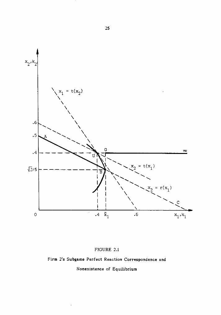
In Figure 2.1, the line ABC is firm2’s

Cournot reaction function, x2 -

r(x1) == .5 — .5}:1, computed with a constant marginal cost of V-§—R = 1. Firm

2’sprofit decreases as we move from left to right along ABC. The lines, xl =

t(x2) = .6 — .5}:2 and xi == t(x1) = .6 — .5x1, are firm l's and firm2’s

Cournot

24

reaction functions, respectively, with a constant marginal cost of V =· .8.

Point U is their intersection: (xl], xg) ·· (.4, .4). Firm2’s

isoprofit curve

passing through point B, computed with a marginal cost equal to 1, is tangent

to the line xl - t(x2) at point U. Firm2’s

profit on that isoprofit curve is

.08.

Now firm l chooses kl in the first stage and firm 2 chooses kg in the

second stage, both exercising perfect foresight about the actions in future

stages. In the third stage both firms engage in capacity·constrained Cournot

competition, given the capacities.

We first focus on firm2’s

subgame perfect reaction correspondence.

lndeed, for kl 2 .4, if firm 2 chooses a capacity kg • .4, then the equilibrium

of the (kl, .4) subgame will be (xrlj, xg) and its profit will be .08. But for kl

in the interval [.4, kl), with kl =- (5-24-2)/S) ¤¤ .4343, it can make more profit

by choosing kg - r(kl). Then, the equilibrium of the (kl, kg) subgame is

§1(k1, kg) - kl, §1(k1, kg) - kg. More generally, for any kl < kl, firm 2 will

choose a capacity r(kl). These best responses of firm 2 are represented by

the segment [A, B) in Figure 2.1.

For kl > kl, on the other hand, firm 2 is better off by choosing kg — .4

and its best responses are given by the half line (G, ¤<>). For kl — kl, firm 2

has two best responses, r(kl) =· J2/5 and .4. As a consequence, firm2’s

subgame perfect correspondence comprises the union of [A, B] and [G, <>¤).

We can now study firm l’s choice of a capacity. Clearly, it will not

choose a capacity greater than i21• This is so since such a capacity will

result in (.4, .4) as the Cournot-Nash equilibrium in the third stage and thus

firml’s

profit with the capacity is smaller than that with, for example,

25

X2’X2 _

\ -\ X1 ’ I’IX2I ’\\\\\

.6 \ \\\\\ \

.5 A \ \\\ \\x\\

G

I \I\\\x = t(x )

I I \ \\I \ \ x2 = r(xl)

II \I I \\ \ \ CI I \ \\

O .4 kl .6 xl,I«:l

FIGURE 2.1

Firm2’s

Subgame Perfect Reaction Correspondence and

Nonexistence of Equilibrium

26

kl = .4. It is easy to show that the profit of firm 1 is increasing in kl on the

interval [0, kl): it increases as we move down from point A to point B along

the segment [A, B) in Figure 2.1. Indeed, it reaches a maximum when firm 1

chooses kl and firm 2 chooses which corresponds to point B.

Thus if firm 1 expects firm 2 to choose a capacity of r(kl) when confronted

with kl, then it will choose kl. However, if firm 1 expects firm 2 to choose .4

instead of r(kl) as a response to kl, then it cannot find its best capacity and

we would not have an equilibrium. To avoid this problem, we introduce the

following assumption.

Assumption 1. In the km subgame, if E(km)> 0, then firm m+1 chooses the

smallest of its best response capacities, min A(km).

By Definition 7 and Assumption 1, we can write Em+1 as a function of

km, km+l(km), in the km subgame.

Definition 9. Let Hl(k"‘+1) - il(km+1) f(Y(km+1)) — Cl( il(km+1), kl), for i€M.

The capacity-output combination (km-H, §m+1) is a subgame perfect Nash

equilibrium of the full game if

ng E'", E„,+lcE“‘> > 2 n,«1Z1'}, 14,), E„,„.ln2{‘}, kl); for an ki 2 o and rar an lem,

EI-n+1 " and

E, = gl im, 2„,+,¤z‘“>> for all lem.

27

We show that in all subgame perfect equilibria all firms are constrained.

Thus in this model, incumbent firms cannot deter entry by holding capacities

that will be unused after entry. For future reference, we first establish the

following.

Lemma 14. Given a capacity combination of the other incumbent firms kg,

firm i with iEM never chooses a capacity ki such that it is nonconstrained in

the equilibrium of km subgame.

‘.Suppose that given kg, firm i chooses a capacity, ki, such that it is

nonconstrained in the km subgame (i&L(km, km+i(km))). We show that the

capacity is not its best response to the capacity vector of the other

incumbent firms: there exists ki > 0 such that IIi((k2, ki), ki)) >

lIi(km, km+i(km)). Indeed, let ki -§i(km, km.i.i(km)). Then ki < ki since

iettkm, Emiiikmii.

We first show that kiii.i,i(kE, ki) g km.i.i(km). Suppose on the contrary

that km+i(ki‘}, ki) > km.i.i(km). Since i€D((kE, ki)), km+i(km)), we have

ki), km+i(km)) = §ii(km, kiii+i(km)) for all JET/I- (see Lemma 4 (b)) and

thus l”l((k¥;, ki), km+i(km)) - H(km, km.i,i(km)). We also have

l”I((kE, ki), ki)) > Il((k?i, ki), kii.i+i(km)). It follows from the facts

that ki) is the mininum of best responses of firm m+l to (kg, ki) and

Emickß, ilii >1Em+i(k“‘>.

Next, iizpttkfi, Ei), 1E„,+1<1J">> and 1Zm+1<k['i, 12,) >km.i.i(km) result in ki), km+i(km, ki)) (see Lemma 4 (c)), which implies

with ki < ki that §i((l·;f‘;, ki), ki)) —§ii(km, ki)) for all

j€!7l

(see Lemma 4 (b)) and thus ki), ki)) =-

28

Hence II(km, Em.,1c12§, 12i)) > 11<12‘“, 12m+1(12“‘)), which aamadiaia that im+i(12"‘)

is a best response of firm m+1 to km.

Second, X((kP;, ki), ki)) g X(km, km+i(km)) since ki < ki and

ki) g km+i(km) (see Lemma 4 (e)).

Third, IEL((k2, 121), E„,+1(12['}, 12i)) since iEL((k2, 12i), 12„,+1c12'“)) andki) g km+i(km) (see Lemma 4 (c)).

rhua,The

last two results imply that

Hi(km, 12„,+1(12“‘)). o.1a.1>.

Proposition 1. In each subgame perfect equilibrium, all firms are constrained.

I‘.The proposition is established by Lemma 9 and Lemma 14.

Consider a market situation where m incumbent firms, each with a

constant marginal cost of V-}-R, engage in Cournot competition. Sincef’(X)

exists and is negative on the interval [0, X), the Cournot equilibrium is unique

(see Szidarovszky and Yakowitz (1982)). By symmetry, the Cournot

equilibrium output of firm i,i€M,

is the same as that of firm j, JEM. Let xc

be the Cournot output of firm i, iEM, and XC- mx¢.

We show in the following proposition that whenever there is an entry-

preventing equilibrium, there always exists a unique symmetric equilibrium. It

is obvious that in the case where E(k„T) > 0, there is no entry-preventing

equilibrium.

29

Proposition 2. Consider the case where E(kg) g 0. (a) If Y g XC, then

((k°)m, 0) is a unique symmetric entry-preventing equilibrium (capacity vector)

where (k°)m — km with ki — xc for all i€M.6 (b) If Y >X° and there is an

entry-preventing equilibrium, then ((Y/m)m, 0) is the unique symmetric entry-

preventing equilibrium.

'. Proof of part (a). We show that ((kc)m, 0) is an equilibrium. First,

km+i((k°)m) - 0 since E(kE) g 0 and Y g X° imply that E((k°)m g 0. Second,

it is easy to show that for iEM, Hi((kc)m, 0) 2 Hi(((kc)I'i, ki), 0) 2

Hi(((kc)P;, ki), kiii+i((kc)2, ki)) for all ki 2 0. It is easy to show that there is

no other symmetric entry-preventing equilibrium.

Proof of part (b). Let (km, 0) be an equilibrium and ki - max (ki, , km).

Then L(km, 0) - Ü by Proposition 1 and Ei£M ki - Y since Y > XC. Suppose

that ((Y/m)m, 0) is not an equilibrium. Since kiii+i((Y/m)m) - 0 (see Lemma 11),

it implies that there exists ki such that IIi(((Y/m)2, ki), ki)) >[li((Y/m)m, 0). Trivially, Y/m > ki since Y >

XC. By Lemma 13,

ki) - r((m-1)Y/m + ki) and L(((Y/mf}, ki), ki)) - Ü.

Next, let ki be such that EiEM\iii ki + ki - (m-l)Y/m + ki. Then ki < ki

since ki < Y/m. Since ki < ki, EFM ki - Y, and km+i(km) - 0, by Lemma 12

E,„„.,112[‘}, 12,) - iixigiviiiii ki + 12,) and 11114*}, 12,), 12„,„.,112[*i, 12,)) - 171.Thus we have the following: X(((Y/m)P}, ki), ki)) =·

X((kE, ki), ki)) - X, since all firms are constrained in both cases,

EisM\iii ki —+- ki - (m-1)Y/m + ki, and kiii+i((Y/mm, ki) - ki).

Notice that ki — Y/m - ki — ki > O.

30

We are now prepared to show that Hi((k2, ki), ki)) > l”Ii(km, 0),

which contradicts that (km, 0) is an equilibrium. The profit of firm i in the

equilibrium of the (ki'}, ki) subgame is ki), ki))

- ki(f(Y)—V——R) - ki(f(}?)—V—R) + (ki — ki)(f(}?)—V—R)

- l'li(((Y/mg}, ki), km.i.i((Y/m)¥i, ki)) -4- (ki — l::i)(f(Y)—V—R) and Hi(km, 0) -ki(f(Y)—V—R) - Y/m(f(Y)—V—R) -4- (ki - Y/m)(f(Y)—-V—R) =- IIi((Y/m)m, 0)

-4- (ki — Y/m)(f(Y)—V—R). Since we have been assumed that

Hi(((Y/m)2, ki), ki)) > Hi((Y/m)m, 0) which also implies that f(Y)

< f()_Ö with the facts that L((Y/m)m, 0) - Ü (see Lemma 11),

ki), ki)) - 17, and Y/m > ki, thus

Ili((kP;, ki), ki)) > IIi(km, 0). It is easy to show that there is no

other symmetric entry-preventing equilibrium. Q.E.D.

Consider now a two-stage game where in the first stage m incumbent

firms decide independently how much to produce and in the second stage firm

m+1 chooses an output, taking the incumbents’ outputs as given. Let F - 0

and let V—4—R be the constant marginal cost of each firm. Notice that firm

m+1 produces r(Q) where Q is the total output of the incumbent firms. Thus

s(Z), the best response of an incumbent firm when the other incumbent firms

produce a total output of Z, is defined as follows.7

Definition 10. Let s(Z) - argmgäo xf(Z-4-x-4-r(Z-4-x)) — (V -4-R)x for ZE[0, <>¤).

It is easy to show that given our assumptions, s(·) is continuously

differentiable and -1 <s’< 0 for Z such that s(Z) > 0. Let g(Q) - f(Q -4- r(Q)).

31

Since g’(Q) exists and is negative on [0, X), the equilibrium of the two-stage

game is unique (see Szidarovszky and Yakowitz (1982)). By symmetry, the

equilibrium output of firm i, iEM, is the same as that of firm j, jEM. Let xs

be the equilibrium output of firm i, iEM. Then r(mx$) is the equilibrium

output of firm m+1.

s(Z) can be interpreted, in our three-stage game, as the best response

(capacity) of firm i, i€M, to a capacity vector of the other incumbent firms,

(ki)\i€M\ii} with Z - Zj€M\iii ki, under the conditions that kiii+i(km) -r(Z+ki) and L(km, kiii.i.i(km)) = I71 where ki - s(Z).

Proposition 3. Consider the case where E(k,T) g 0. If Y >XC, then either

((Y/m)m, 0) or ((kS)m, k?ii+i) is an equilibrium where (ks)m -km with ki ·-

xs

for all iEM and kiwi - r(mxs).

‘.It is obvious that when Y g mxs, ((Y/m)m, 0) is an equilibrium.

Consider the case where Y > mxs. Suppose that neither is an equilibrium.

Since ((Y/m)m, 0) is not an equilibrium and kiii.i,i((Y/m)m) =- 0 (see Lemma 11),

for some iélvi there exists ki such that Hi(((Y/m)E, ki), kiii.i.i((Y/m)?;, ki)) >

l”Ii((Y/m)m, 0). We have Y/m > ki since Y > XC. By Lemma 13,

kiii+i((Y/m)?i, ki) = r((m—1)Y/m + ki) and L((Y/m)?;, ki), kiii.i,i((Y/m)T;, ki)) - Ii-/1.

Since l”Ii(((Y/m)E, ki), ki)) > IIi((Y/m)m, 0) and Y/m > ki, X -

X(((Y/mm, ki), ki)) < Y. We show that L((kS)m, k?ii,i.i) - Ü. It

is trivial that m+1•EL((kS)m, käiiii). Since mks < Y and thus II((kS)m, k?ii.i.i)

2 0, if j<ZL((kS)m, kiwi) for some jEM and thus all incumbent firms are

nonconstrained (see Lemma 3 (b)), then E(K„T) 2 II((kS)m, k?ii+i) > O (see Lemma

32

which contradicts that E(12.‘P) S 0. Now that (ucs)'", k§,+,) is lnot an

equilibrium and L((kS)m, ki$ii.i,i) - l7I, we should have the following:

12,), E„,+,1112S)['i, 12,)) - M and 12,), 0) > 11,1112S)“‘, 12§i+i) whereki - Y—1m-1)12S.

Choose ki such that (m—1)kS -1- ki - (m—1)Y/m -1- ki. Then ki > ki

since 12S < Y/m. Since ki > 12,, 1m-1)12S + ki - Y, and 12,) - 0,by Lemma 12 we have 12„i+i((kS){'}, ki) - r((m—1)kS -1- IE,) - r((m—1)Y/m -1- ki)

aha L(((kS)Pi, 12,), E,,,„.,1112S)['i, 12,)) - 171.Notice that E - i(((kS)2, 12,), E„,,,,1112S)§, 12,)).

We are prepared to show that IIi(((ks)2, ki), ki)) >

Hi(((kS)I';, ki), 0). The profit of firm i in the equilibrium of the ((kS)E, ki)

subgame is IIi(((kS)2, 12,), 12„,,,,1112S)§‘}, 12,)) - 12,1102)-v-12) - 12,002)-v—12) +(ki—ki)(f(Y)—V—R) - 11,111Y/m){‘}, 12,), 12,,,.,,11Y/m)¥i, 12,)) + (ki—ki)(f(Y)—V -12)and Üi(((kS)2, ki), 0) - ki(f(Y)—V —R)

- Y/m(f(Y)—V—-R) +112,-12,)111Y)-v-12) - 11,11Y/m)“‘, 0) + 112,-12,)11·1Y)-v-12)since ki - Y — (m—1)kS - Y — ((m—1)Y/m + ki — ki) - Y/m -1- (ki — ki).

Since Hi(((Y/n1){’i, ki), 1€„i.,.i((Y/mf'}, 12,)) > IIi((Y/m)“‘, 0) and NI?) > f(Y), we

have Hi(((kS)E, 12,), 0) S Hi(((kS)1Ti, 12,), 2„,,.,1112S)[‘i, 12,)) S Ui((kS)m, 12;+,), whichis a contradiction. Q.E.D.

Now consider the case where E(kT) > 0. Incumbent firms have no

choice but to accommodate firm m+1. Let 2* 2 0 be such that

r(2*)f(2*-+—r(2*)) — (V-1-R)r(2*) — F - E(k,T). By Lemma 1 (d), it is unique.

In our three-stage game, 2* can be interpreted as the sum of incumbents’

capacities, ZMM ki, which yields the profit of E(kE) to firm m+1, if firm m+1

33

chooses km+1 = r(Z*) and L(km+1) = Ii. Let kE- 2*/m and käi.1 - r(2*).

Lemma 15. Let (kE)m -km where ki — kE for all iEM. In the equilibrium of

the (kE)m subgame, firm m+1 chooses k§i+1 and all firms are constrained.

Proof. It is easy to show that k§i+1 - min A((kE)m). Then it follows from

Assumption 1 that km+1((kE)m) -· kä+1.

We show that in equilibrium all firms are constrained. We have m+1 E

L((kE)m, kä.1,1) since kä+1 - r(2*) < t(2*) g t(m>T:) where i - äi((kE)m, kä+1)

for all i€M (see Lemma 3 (b)). Suppose that iQL((KE)m, 1%:1+1) for some i€M.

Then j<;EL((kE)m, kä.1,1) for all jEM (see Lemma 3 (b)) and m§<ml<E - 2*.

I-lence H(k,T, 1%,1) = 11«1.E)’“, 1%+1) - 1%,11 f(m§+k§i+i)—V—R) - 1= >

k§·i+1( f(2*+kä+1)—-V—R) — F-

E(k§), which is a contradiction. Notice that

the first equality comes from Lemma 4 (b). Q.E.D.

I-Ience the profit of firm m+1 in the equilibrium of the (kE)m subgame

equals that in the equilibrium of the kg subgame, i.e. II((kE)m, kä+1) - E(k.T).

Proposition 4. Consider the case where E(kE) > 0. (a) If ks< kE, then

((ks)m, ksii+1) is a unique symmetric (entry-allowing) equilibrium. (b) If ks2

kE, then under Assumption 1, ((kE)m, 1%+1) is a unique symmetric (entry-

allowing) equilibrium.

Proof. Proof of part (a). We have L((ks)m, käi.1,1) - Ü. It follows from the

facts that (ks)m< (kE)m, ksn+i = r(mks), kä+1 - r(mkE), and by Lemma 15

34

L((kE)m, käi,1) · Ü, and from Lemma 5.

We first show that km.i.1((ks)m) - ksiii,1. Obviously, lI((ks)m, käi+1) >

1I((kS)’“, 11,,,+1) for kiii+1 2 0 such that kiii+1 e-6 k§i+1 and L((kS)"‘, kiii+1) - M.

For ki.ii.i,1 such that E < ks where E - ii((ks)m, kmi,1) for all iEM (see Lemma

6 (11)), Il((ks)m, k„i+1) - l'I(k.T, 11,,,+1) g E(kP,‘) - 11((kE)"‘, ki§i+1) <l'I((ks)m, ksii.i.1). The first equality comes from Lemma 4 (b) and the last

inequahty follows from the fact that L((kE)m, k§+1) - L((1<S)"‘, k§i+1) - 17 andks

< kE, and from Lemma 1 (d).

Next, consider firm 1, 16114. Far ki < ks, IIi(((ks)2, ki), kiii+1((ks)§, ki))

< l'Ii((ks)m, ksiii.1) since kiii+1((ks)Pi, ki) - r((m—1)ks -1- ki) by Lemma 11 and

L(((ks)Pi, ki), kii.i+1((ks)£, ki)) — l7l by Lemma 5 (and the definition of ks). By

Lemma 14, firm i will not choose ki such that iEL(((ks)Pi, ki), ki)).

For ki > ks such that i E L(((ks)¥i, ki), kiii+1((ks)Pi, ki)) and thus all firms are

constrained (see Lemma 3 (c) and Lemma 8),

Hi((ks)m, ksii+1) > Hi(((ks)1‘i, ki), k„i+1((ks)§, ki)) by the definition af ks.It is easy to show that there is no other symmetric equilibrium.

Proof of part (11). By Lemma 15, L((kE)'“, kiiEi+1) - M and 1E„i+1((kE)"‘) - k§i+1.We must show that firm i, i€M, has no incentive to choose a capacity other

than kE, given (kE)Pi. Indeed, for ki < kE, since kiii+1((kE)Pi, ki) -r((m—1)kE + ki) by Lemma 11 and thus L(((kE)§, ki), kiii+1((kE){'i, ki)) - M by

Lemma 6, we have 1ii((kE)'“, k§i+1) > IIi(((kE)£, ki), k„,+1((kE)¥}, ki)) from thefact that kE g ks. Suppose that ki> kE. Then kiii+1((kE)?i, ki) -km+1(kI.P) and § < kE where 11 - §_i(((kE)§, ki), kiii+1((kE)[‘i, ki)) for all 36M.

Since Y((kE)‘“, 1%+1) < )?((kE)'“, Eiii+1(k.'i‘)) - i(((kE)§, ki), 12„,+1((kE){‘i, ki))

35

(see Lemma 4 (e) and (b)), we have IIi((kE)m, k§i+i) >

Hi(((kE)E, ki), ki)). It is easy to show that there is no other

symmetric equilibrium. Q.E.D.

Propositions 2, 3 and 4 established the existence of an equilibrium of the

full game by constructing symmetric equilibria. As we will see in the sequel,

if E(k.T) g 0 there might exist two disconnected symmetric equilibria where

one is entry-allowing and the other is entry-preventing. It can also be shown

that when E(k.T) g 0, there might exist a continuum of entry-preventing

equilibria, each yielding the same total output. This result can also be found

in Bernheim (1984) and Gilbert and Vives (1986). What is new in this essay is

that in this strategic entry deterrence model there might exist a continuum of

entry-allowing equilibria. It happens when E(k.T) > 0 and kE<

ks. ln the fol-

lowing example, there is a continuum of entry-allowing equilibria among which

° the total output of incumbent firms (and the total output of all firms) is notl

constant. Furthermore, we show in the example that in some equilibria the

profit (market share) of an entrant is larger than that of an incumbent firm.

Example 2. There are two incumbent firms, called firm 1 and firm 2, and one

potential entrant, firm 3. Hence FTI = {1, 2, 3}. The inverse demand function is

given as follows: p -f(X)

- 2 — X for 0 g X g 2 and p -= 0 for X > 2. Let

V == .9, R = .1, and FE [0, 77/1600).

It is easy to show that given kg, A(k?.) - {.275). Since ?<i(k?., kg) ··

§i(k?., .275) = .275 for all iEl7I, E(k?.) - II(k?,, .275) - 77/1600 — F > 0 and

thus k3(kg,) = .275. E(k?.) > 0 implies that E(k2) > 0 for every capacity

36

vector kg and thus k3(k2) > 0: that is, firm 3 always enters.

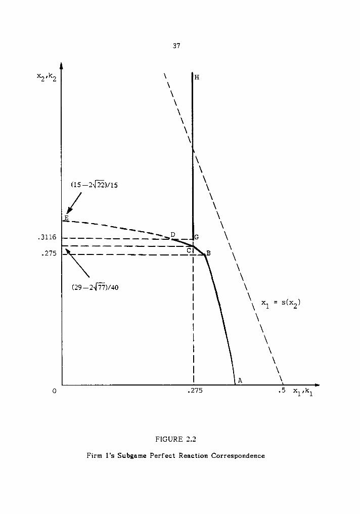
To get the subgame perfect reaction correspondence of firm 1, focus

first on the maximum capacity, denoted by kl, that firm 1 can choose, given

kg, satisfying that L(kl, kg, k3(kl, kg)) - Ü. Notice that L(kl, kg, k3(kl, kg)) ·171 implies that k3(kl, kg) · r(kl+kg). Hence kl is implicity computed as

follows. For kg E [0, .275], E(c¤, kg) - H(kl, kg, k3(kl, kg)) -

r(kl+kg)[f(kl+kg+r(kl+kg)) — 1] —· F. Since E(o<>, kg) =- (.8—kg)(1.1—kg)/9

— F and ll(kl, kg, E3(Rl, kg)) = (1 —kl-kg)2/4 - F, then (.8-kg)(1.1-kg)/9 =

(1 -kl—kg)2/4. The relation is represented by the locus AB in Figure 2.2.

That is, AB shows kl given kg E [0, .275]. For kg E [.275, (29-2];)/40],

E(¤¤, kg) = E(k.?.) = 77/1600 - F = (1 —kl—kg)2/4 - F. We have 77/1600 =

(1-kl-kg)2/4, which is represented by the locus BC in Figure 2.2. For kg E

[(29-2]%)/40, (15-257)/15], E(kl, <>¤) = (1-kl—kg)2/-l — F. Since E(kl, cs)

= (.8—kl)(1.1-kl)/9, it gives us (.8—kl)(1.1—kl)/9 = (1—kl—kg)2/4. The

relation is represented by the locus CDE in Figure 2.2. For kg >

kl does not exist, but for convenience of exposition let kl - 0.

Next, notice that for kg > (29—2~]-T7)/40, firm 1 is constrained in the

third stage if it chooses a capacity between kl and .275. But firm 2 is

nonconstrained in that case. l'Il(.275, kg, k3(k2)) > l”Il(kl, kg, 1-(-3(lzl, kg)) for all

ill +2 (ill, .275).

Now we are prepared to derive firm 1’s reaction correspondence. First,

for kg E [0, (15-245)/15], Hlüzl, kg, k3(kl, kg)) > l'Il(kl, kg, k3(kl, kg)) for all

kl E [0, kl) since xl = s(x2) =- .5 — .5x: > kl, given kg - xi. Notice also

that by Lemma 14, firm 1 never chooses a capacity which results in excess

capacity in the third stage. Thus, for kg E [0, (29—2«l?7)/40], since kl is also

37

Xzrkz \ H\\\\\\\

\\

(15—2@)/15 \\\

E — \_

® T ä —

—.3116.....--...‘:..>D _ G \——————— ———— \.275 - ....-......CL B \I1 \I \

(29-2JW)/40 I \xl = s(x2)

I \I \I \I xI \I \I A \

0 .275 .5 xl,kl

FIGURE 2.2

Firm1’s

Subgame Perfect Reaction Correspondence

38

the maximum capacity firm 1 can choose without resulting in excess capacity,

ill is the best response of firm 1. For kg > (29-2~l?7)/40, firm 1 compares

IIl(kl, kg, k3(kl, kg)) with Hl(.275, kg, k3(k2)) and chooses that capacity which

yields the highest profit. Firml’s

profit decreases as we move from right to

left along CDE and Hl(kl, kg, E3(E1, kg)) ·· Hl(.275, kg, k3(k2)) when kg is equal

to .3116 (point D in Figure 2.2). Hence, for kgé [(29-2m)/40, .3116], firml’s

best response is kl and for kg 2 .3116 it is .275. In Figure 2.2, ABCD and GH

are firm1’s

reaction correspondence.

The subgame perfect reaction correspondence of firm 2 is obtained in a

similar way. Let kg be the maximum capacity firm 2 can choose, given kl,

satisfying that L(kl, kg, kg(kl, kg)) - Ü. For klE [0, .275], (.8—kl)(1.1—kl)/9

= (1 —kl—kg)2/4, for klE [.275, (29-257)/40], 77/1600 = (1 —kl-kg)2/4, and

for kl G [(29—2~[?7)/40, (15-2E)/15], (.8—kg)(1.1—kg)/9 = (1 -kl—kg)2/4.

For kl > (15-2—l_7?2)/15, kg does not exist. Firm2’s

best response is kg for

kl E [0, .3116] and .275 for kl 2 .3116. Hence, the subgame perfect reaction

correspondence of firm 2 and that of firm 1 are symmetric about the line

x: = xl.

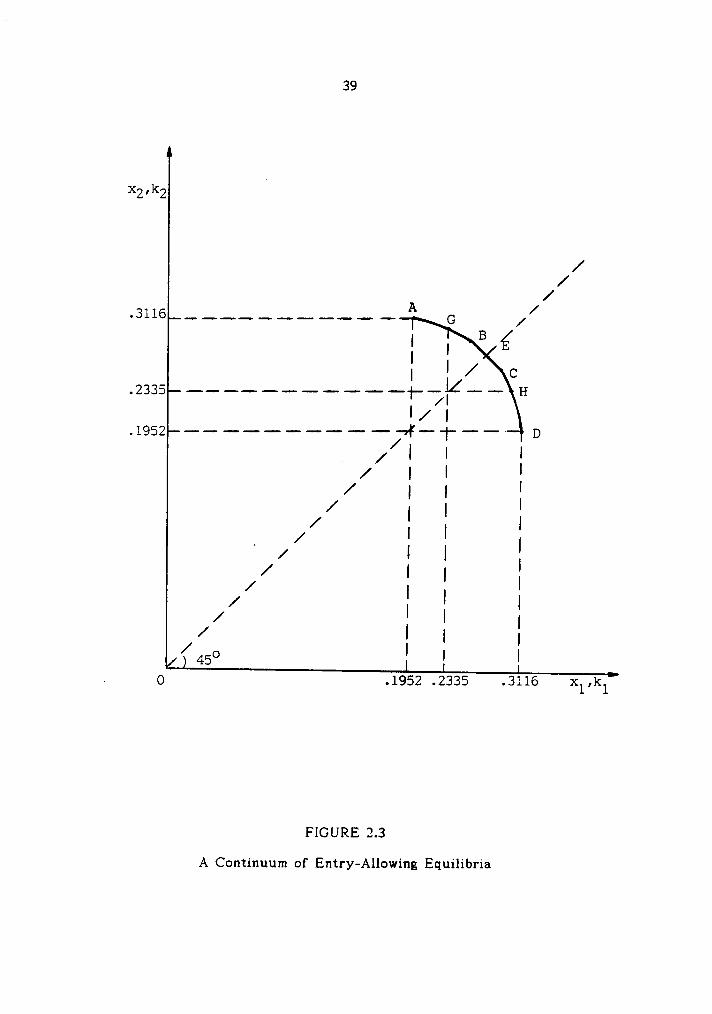
Equilibrium capacity (and output) vectors of firm 1 and firm 2 are shown

in Figure 2.3. Several remarks are in order. First, the total output of the in-

cumbent firms is in general different across the equilibria. lt is the same and

maximal for equilibrium capacity (and output) vectors on BC in Figure 2.3.

Since k3(kl, kg) = r(kl—§-kg), the total output of all firms is also in general dif-

ferent across the equilibria. lt is the same and maximal for (kl, kg) on BC in

Figure 2.3. Second, the capacity (output, or market share) of firm 3 is larger

than that of firm l on AG in Figure 2.3 and is larger than that of firm 2 on

39

x2·I‘2

///.3116 ____.___..

-A G //

I I B {II I / C

.2335 HI / I

.1962 ———————————»¥——I--——·— D/ I I I/ I/ I I/ I I I/ I I/ I I. / I I/ I I I/ I I/ I I

I/ I I/ I I/ I I I

/450 I I II 0 .1952 .2335 .3116 xI,kI

FIGURE 2.3A Continuum of Entry-Allowing Equilibria

40

HD in Figure 2.3. It can be easily verified that the profit of firm 3 can be

larger than that of firm 1 or firm 2. For example, if F = 0, the profit of firm

3 is larger than that of firm 1 on AG and that of firm 2 on HD in Figure 2.3.

Third, the capacity vector (F1, F2, F3(F1, F2)) when (Fl, F2) is at E in Figure

2.3, is equivalent to ((kE)m, kä.,1) in Proposition 4.

S. POSSIBLE UNDERINVESTMENT IN ENTRY DETERRENCE

Entry deterrence has the characteristics of a public good. Entry preven-

tion by a group of incumbent firms protects all incumbent firms from the new

competitor and makes all incumbent firms better off. That is, "consumption"

of entry deterrence is not exclusive. Now, the incumbent firms in this model

cannot collude on an investment in entry deterrence. That is, they cannot

coordinate their choice of capacities in the first stage. Thus, the free rider

problem of a public good suggests that in our model there would be an

underinvestment in entry deterrence.

Gilbert and Vives (1986) consider a two—stage model in which in the first

stage incumbent firms decide independently how much to produce and in the

second a potential entrant decides whether or not to enter the industry and if

it enters how much to produce, taking the total output of the incumbent firms

as given. They show that even if the incumbent firms cannot collude when

they decide on quantities they will produce and thus the free rider problem

suggests that the incumbent firms would tend to underinvest in entry

deterrence, there is no underinvestment in entry deterrence in their model.

41

They associate an underinvestment in entry deterrence with one or more of

the following:

(a) incumbents’ total profits are higher when they prevent rather than allow

entry, but the (unique) industry equilibrium allows entry.

(b) Either entry prevention or entry may be an industry equilibrium, but

incumbents’ profits are higher when entry is prevented.

(c) An established monopoly (or colluding incumbents) prevents entry in more

situations than an established, noncooperating, oligopoly. (Gilbert and

Vives (1986), p. 77)

At a glance, one may argue that since all incumbent firms are constrained

in a subgame perfect equilibrium of our three-stage game (see Proposition 1),

our three-stage model reduces to the two-stage model of Gilbert and Vives

(1986), and may conclude that there is no incentive to underinvest in entry

deterrence in our model. However, this reasoning is not correct. Notice that

while it is always possible, in their model, for each incumbent firm to prevent

entry, given the other incumbent firms’ outputs, this is not the case in our

model. There is no capacity vector of the incumbent firms that prevents

entry when E(k.T)>0. Even when E(k,T)g0, there are situations where an

incumbent firm would be better off keeping a potential entrant out, given the

other incumbent firms’ capacities, but it is not feasible for it to do so. This

outcome follows from the fact that a potential entrant ignores capacities that

are not going to be used after it enters. That is, it ignores noncredible

threats made by the incumbent firms. lndeed, the following example shows

42

that there may be an underinvestment in entry deterrence in our model. In

the example, there are two disconnected symmetric equilibria: one is entry-

preventing and the other is entry—a1lowing. Incumbents’ profits are higher

when entry is prevented (see (b) in the previous page), which also implies that

colluding incumbents prevent entry but noncooperating incumbents may not do

so (see (c) in the previous page).

Example 3. There are two incumbent firms, firm 1 and firm 2, and a single

potential entrant, firm 3. The inverse demand function is given by: p — f(X)-

1.2 —Xfor0 gX g1.2andp=0forX >1.2. Let V=.92,R=.08,andF

= (.013)2.Suppose that in the first stage both incumbent firms choose infinite

capacities. Let kg be firm 3’s capacity chosen in the second stage. Firm 3

does not choose a capacity which is not going to be used fully in the third

stage. In the third stage, since the incumbent firms are nonconstrained and

firm 3 is constrained, xl - t(x2+kg) =· .14—.5x:—.5kg, xi. = t(x1-1-kg) =

.14—.5x1—.5kg, and x3 = kg, which imply that §1(k:;, kg) = §_g(k£,, kg) =

7/75-kg/3. Firm 3, exercising perfect foresight with respect to the outputs

of the incumbent firms, chooses a capacity which is an element in A(k?,).

Mkt?.) = {1/50}. Since iT:1(k?., 1/50) = §2(k;;?„, 1/50) = 13/150 and >T:g(kl;2., 1/50) ·1/50, E(kg,) = H(k.;3,, 1/50) = 1/7500 — F < 0. Hence, if both incumbent firms

choose "sufficiently large" capacities, firm 3 will not enter the industry.

The limit output Y has the value of .174 (see Definition 8) and is larger

than the sum of the full cost two-firm Cournot equilibrium outputs: XC = 2xC

= 2/15. There is then at least one symmetric equilibrium.

43

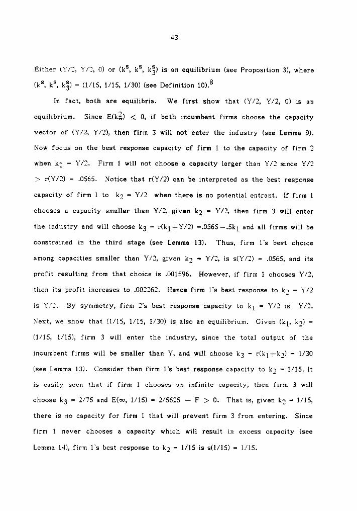
Either (Y/2, Y/2, 0) or (ks, ks, kä) is an equilibrium (see Proposition 3), where

(ks, ks, kg) = (1/15, 1/15, 1/30) (see Definition 10).8

In fact, both are equilibria. We first show that (Y/2, Y/2, 0) is an

equilibrium. Since E(kg.) g 0, if both incumbent firms choose the capacity

vector of (Y/2, Y/2), then firm 3 will not enter the industry (see Lemma 9).

Now focus on the best response capacity of firm 1 to the capacity of firm 2

when kg = Y/2. Firm 1 will not choose a capacity larger than Y/2 since Y/2

> r(Y/2) = .0565. Notice that r(Y/2) can be interpreted as the best response

capacity of firm 1 to kg - Y/2 when there is no potential entrant. lf firm 1

chooses a capacity smaller than Y/2, given kg - Y/2, then firm 3 will enter

the industry and will choose kg = r(kl—l-Y/2) -.0565-.5kl and all firms will be

constrained in the third stage (see Lemma 13). Thus, firm 1's best choice

among capacities smaller than Y/2, given kg - Y/2, is s(Y/2) = .0565, and its

profit resulting from that choice is .001596. However, if firm 1 chooses Y/2,

then its profit increases to .002262. Hence firm 1’s best response to kg = Y/2

is Y/2. By symmetry, firm2’s

best response capacity to kl =- Y/2 is Y/2.

Next, we show that (1/15, 1/15, 1/30) is also an equilibrium. Given (kl, kg) =

(1/15, 1/15), firm 3 will enter the industry, since the total output of the

incumbent firms will be smaller than Y, and will choose kg = r(kl—%-kg) = 1/30

(see Lemma 13). Consider then firm1’s

best response capacity to kg =· 1/15. lt

is easily seen that if firm 1 chooses an infinite capacity, then firm 3 will

choose kg = 2/75 and E(o¤, 1/15) - 2/5625 — F > 0. That is, given kg = 1/15,

there is no capacity for firm 1 that will prevent firm 3 from entering. Since

firm 1 never chooses a capacity which will result in excess capacity (see

Lemma 14), firm 1's best response to kg = 1/15 is s(1/15) = 1/15.

44

By symmetry, firm2’s

best response to kl =- 1/15 is 1/15.

The profit of each incumbent firm is .002262 at the symmetric entry-

preventing equilibrium and 1/450 at the entry-allowing equilibrium. It is

higher when entry is prevented than when entry is allowed.

6. COMPARATIVE STATICS

In this model an increase in the number of incumbent firms, m, makes

entry prevention more plausible. This is so since by increasing the number of

incumbent firms, on one hand entry prevention may become feasible in the

sense that E(k.T) becomes nonpositive (see Lemma 4 (e) and Definition 5), and

on the other hand competition among incumbent firms becomes more intensive

and reduces the profitability of allowing entry, relative to preventing entry.

An increase in the fixed cost of entry, F, also increases the possibility of

entry prevention since it may make entry prevention feasible by reducing the

value of E(k.T) and it decreases the limit output, Y. Let ot be the proportion

of the capacity cost to the full cost: ot -R/(V4-R). We then have 0<otg1.

Notice that entry prevention becomes more likely with an increase in ot when

V+R is constant, since this decreases E(k,T). The parameter ot can be

interpreted as a measure of the degree of strategic advantage held by incum-

bent firms (or first movers).

ln the sequel, we first show that when there is a single potential entrant

the feasibility of preventing entry does not imply the existence of an entry-

preventing equilibrium.9 We then examine how an increase in the number of

45

incumbent firms and a decrease in the cost of entry affect both equilibrium

prices and welfare. It is shown that an increase. in the number of incumbent

firms can raise the equilibrium price and lower (consumer) welfare. This

result was also found in the model of Gilbert and Vives (1986, p. 80).

However, in their model if we focus only on the equilibria which yield higher

profits to incumbent firms, then the market price is monotone nonincreasing in

the number of incumbent firms. As we will see, this is not the case in our

model. Reducing the cost of entry may also increase the equilibrium price. In

this case, a decrease in the cost of entry causes a switch from an entry-

preventing equilibrium to an entry-allowing one. Welfare declines due to the

cost of entry incurred, as well as lower total output. Finally, we show that a

decrease in demand may raise the total equilibrium output.

The inverse demand function is assumed to be linear: p - f(X) - a — bX

for 0 g X g a/b and 0 otherwise, with a > 1. Let V-i—R -1. Then R =- on

and V = l—<x. We focus on symmetric equilibria.10 Notice, however, that our

conclusions below do not depend on this choice. The process of finding

symmetric equilibria to this specific model is described below (see the last

three propositions). First, we compute E(k,T). lf E(k,T) > O, then ((kS)m,

k?n+1) is the unique symmetric equilibrium if ks< kE and ((kE)m, kä.,1) is the

unique symmetric equilibrium if ks2 kE. For E(k.T) g 0, we derive the

value of the limit output Y. If Y g Xc- mx¢, then ((kc)m, 0) is the unique

symmetric equilibrium. Otherwise, both ((Y/m)m, O) and ((kS)m, kär,.1) should be

investigated and at least one of them is an equilibrium. Notice that in this

specific model where the inverse demand function is linear, ks-

x¢. In Appen-

dix B and C explicit solutions, when m -= 1 and m = 2, are provided.

46

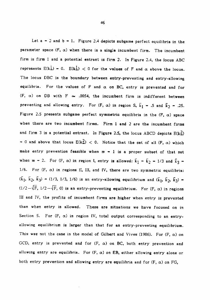
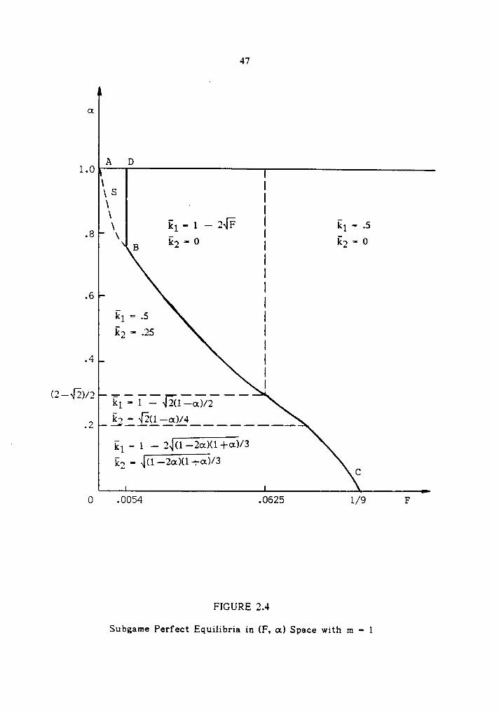
Let a = 2 and b — 1. Figure 2.4 depicts subgame perfect equilibria in the

parameter space (F, on) when there is a single incumbent firm. The incumbent

firm is firm 1 and a potential entrant is firm 2. In Figure 2.4, the locus ABC

represents E(l<},) == 0. E(k}„) < 0 for the values of F and ot above the locus.

The locus DBC is the boundary between entry-preventing and entry-allowing

equilibria. For the values of F and :1 on BC, entry is prevented and for

(F, :1) on DB with F ¤ .0054, the incumbent firm is indifferent between

preventing and allowing entry. For (F, ot) in region S, kl =- .5 and E2 - .25.

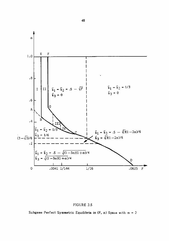
Figure 2.5 presents subgame perfect symmetric equilibria in the (F, :1) space

when there are two incumbent firms. Firm 1 and 2 are the incumbent firms

and firm 3 is a potential entrant. In Figure 2.5, the locus ABCD depicts E(k?.)

= 0 and above that locus E(k?.) < 0. Notice that the set of all (F, ot) which

make entry prevention feasible when m - 1 is a proper subset of that set

when m = 2. For (F, :1) in region I, entry is allowed: kl = 122 = 1/3 and kg =

1/6. For (F, :1) in regions II, III, and IV, there are two symmetric equilibria:

(kl, k2, kg) = (1/3, 1/3, 1/6) is an entry-allowing equilibrium and (kl, k2, kg)

0) is an entry-preventing equilibrium. For (F, 0:) in regions

III and IV, the profits of incumbent firms are higher when entry is prevented

than when entry is allowed. These are situations we have focused on in

Section 5. For (F, :1) in region IV, total output corresponding to an entry-

allowing equilibrium is larger than that for an entry-preventing equilibrium.

This was not the case in the model of Gilbert and Vives (1986). For (F, :1) on

GCD, entry is prevented and for (F, on) on BC, both entry prevention and

allowing entry are equilibria. For (F, :1) on EB, either allowing entry alone or

both entry prevention and allowing entry are equilibria and for (F, :1) on FG,

47

ot

A Dl.O A

I I\ S II .1 I _

8 I kl-1—2~IF I kl-.6„ \ - -

B kg = 0I kg 0

III.6 _ I

kl T .6 |122 T .26 I

I.4 |

II(2—«I3)/2 T — —— ————— 4

kl = 1 — ~E?1——o1)/2

2‘

El = 1 — 2«I(1—2oc)(1—|—<1)/3

kg - „I(1——2on)(1—I-on)/3C

0 .0054 .0625 1/9 F

FIGURE 2.4

Subgame Perfect Equilibria in (F, oc) Space with m = 1

48

ot

1.0E F

IIII .

•8II ' —

1/31 rl-122-.6-~IT=I"1"‘¤’

- kg = 0kg - 0

I.6 I

G IA I

\\ I

.4 B I_ I12 - 12 - 1/3 - -_ E1

136C I kl - kg = .5 — ~I8(1—-20.)/6

(3—«I-3)/6 3:-————————— kg · ‘IE(1—2ü)/6

.2 ————————————

il — E2 - .6 — ,|(1-3¤11<1+¤11/4kg - „I(1·—3o1)(1+o1)/4 D

0 .0041 1/144 1/36 .0625 F

FIGURE 2.5

Subgame Perfect Symmetric Equilibria in (F, on) Space with m =· 2

49

either entry prevention alone or both entry prevention and allowing entry are

equilibria.

In Figures 2.4 and 2.5, the effect of a change in ot on equilibrium

capacities is noteworthy. For a given level of F, the capacities of the

incumbent firms are nondecreasing in ot and the capacity of the potential

entrant is nonincreasing in ot. A change in the parameter ot, the proportion of

the capacity cost to the full cost, has no effect on the full cost but does

affect the credibility of investments in entry deterrence—capacities chosen

by incumbent firms. As ot decreases, incumbent firms lose more and more

credibility of their capacities and thus the difference in capacities between

incumbent firms and the entrant becomes smaller and smaller.

In Figure 2.4, preventing entry is profitable (or desirable) for (F, ot)

when F > .0054 and feasible for (F, ot) on and above ABC. Neither the

profitability nor the feasibility of entry deterrence implies the other. In re-

gion S, E(k},) g 0 but accommodation is the unique equilibrium. This is also

the case in region I in Figure 2.5.

Now consider the effect of a change in the number of incumbent firms m

on the market price and welfare. In our specified model, increasing the number

of incumbent firms from one to two reduces the total equilibrium output over

the wide range in the (F, oc) space. In such cases, the market price rises and

thus consumer welfare falls. This is illustrated in Figure 2.6 which draws on

Figures 2.4 and 2.5. In Figure 2.6, Y1 is the total output when m - 1 and 22

is the total output when m - 2. For (F, ot) on BC, Y1 < YZ and for (F, ot) on

AB or on AD, il = YZ. For (F, ot) on DGH, il > X2. For (F, :1) in the

shaded area, il > YZ if we restrict attention to equilibria which yield higher

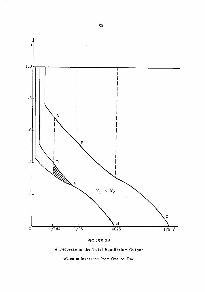
50

Q .

1.0

I II II II II I.8 I II II IA I

III I

.6 I II I

B III

.4 I9 I¢ I Ißß

.2

C

0 1/144 1/36 .0625 1/9 F

FIGURE 2.6

A Decrease in the Total Equilibrium Output

When m Increases from One to Two

51

profits to the incumbent firms. For (F, ot) in other regions, il g ig. The

reason why increasing the competitiveness of the industry has such a

perverse effect is that in our model credibility of capacities increases with an

increase in the number of incumbent firms. For example, when E(k}.) > 0,

there are situations where a single incumbent firm has no choice but to allow

entry, but two incumbent firms prevent entry simply by choosing capacities

equal to the two—firm full cost Cournot output.

In Figures 2.4 and 2.5, a decrease in the cost of entry, F, has no effect

on the total equilibrium output and the market price if entry is allowed at

both values of F. lf entry is prevented at both values of F, the total

equilibrium output is nondecreasing and thus the market price is nonincreasing

when F decreases. However, it is easily seen in both figures that a decrease

in F can cause a decrease in the total equilibrium output and raise the market

price. For example, consider the case where ot - .9 and F decreases from .0064

to .0053 in Figure 2.4. When F = .0064, entry is prevented and the total

equilibrium output is .84 but when F = .0053, entry is allowed and the total

equilibrium output is .75.

Finally, we show that a decrease in demand can raise the total

equilibrium output. Consider the case where m - 1. Let b = 1, ot = .8, and F

= .006. If a = 2.1, then E(k},) > 0 and entry is allowed. The total equilibrium

output is .825 (see Appendix B). But if a — 2, then entry is prevented and the

total equilibrium output is .8451 (see Figure 2.4).

52

7. THE CASE OF MULTIPLE POTENTIAL ENTRANTS

In this section, we assume that there are multiple potential entrants who

choose capacities sequentially, in place of a single potential entrant in the

original model. We first establish that the feasibility of preventing entry

implies the existence of an entry·preventing equilibrium, which was not the

case when there is only one potential entrant. Then, we show in Example 4

that even in the case of multiple potential entrants there may be an under-

investment in entry deterrence.

The m incumbent firms and n potential entrants now form the set of

players in the (n+2)-stage noncooperative strategic entry deterrence game. In

the first stage, m incumbent firms choose capacities simultaneously and

independently, in the second through the (n+1)st stages n potential entrants

choose capacities sequentially, after learning the capacities predetermined, and

in the last stage the firms engage in capacity-constrained Cournot competition,

given the capacities chosen in the first n+l stages. The potential entrant

which decides a capacity in the (i+1)st stage is called firm m+i for i - 1, ,

n. The number of potential entrants, n, is finite and is assumed to be large

enough so that if all m+n firms choose positive capacities, then at least one

firm earns a negative profit.

Let Em.,.i(km+i'1) be the maximum profit that firm m+i can earn if it

enters, given the capacities chosen in the first i stages, km+i'1, and given that

no other potential entrants enter after that firm (see Definition S).

Lemma 16. Firm m+i enters if and only if Em+i(km+i“1) > 0.

S3

The proof is similar to that of Proposition 6 in Eaton and Ware (1987).

Each potential entrant exercises perfect foresight about the actions of the

potential entrants following it when it chooses its capacity. However, Lemma

16 states that as far as entry decision is concerned, each potential entrant can

ignore the existence of the following potential entrants.

Lemma 17. (a) If Em+i(k,T) > 0, then there is no capacity vector of the

incumbent firms that makes all potential entrants stay out. (b)Ifg

0 and all the capacities chosen by the incumbent firms are larger than or

equal to Y/m, then all potential entrants stay out.

The proof is immediate and is omitted. It follows from Lemma 17 that

preventing entry is feasible if and only if Eiii+i(k.T) g 0. We show in the

following proposition that whenever preventing entry is feasible there is an

equilibrium in which all potential entrants stay out.

Proposition 5. If preventing entry is feasible, then ((k°)m, (ki - 0)i8N) is an

equilibrium if Y g XC and otherwise ((Y/m)m, (ki =- 0)i€N) is an equilibrium,

where N is the set of potential entrants.

l‘.The poof of the first part is trivial and is omitted. For the proof of

the second part, notice first that if each of the incumbent firms chooses the

capacity Y/m, then all potential entrants stay out (see Lemma 17 (b)). Next,

consider firm i, i€M, which chooses a capacity, given that all the other

incumbent firms choose capacities equal to Y/m. We must show that given

54

(ki =· Y/m)iEM_i, firm i chooses the capacity Y/m. First, it follows from

Lemma 16 that if firm i chooses a capacity less than Y/m, then entry will

continue until total output is greater than or equal to Y. But if it chooses a

capacity larger than or equal to Y/m, then all potential entrants stay out (see

Lemma 17 (b)). Thus the profit of firm i when it chooses a capacity less than

Y/m is smaller than that with ki - Y/m. Second, firm i will not choose a

capacity larger than Y/m since r((m—1)Y/m) < Y/m. Q.E.D.

I—Ience for the values of F and ot in region S in Figure 2.4, preventing

entry is the only equilibrium when there are multiple potential entrants, while

allowing entry is the equilibrium when there is a single potential entrant. For

(F, oc) in region I in Figure 2.5, there is no entry-preventing equilibrium in the

case of a single potential entrant but there is such an equilibrium in the case

of multiple potential entrants.

In the following example, we show that even when there are multiple

potential entrants, an underinvestment in entry deterrence may arise.

Example 4. There are two incumbent firms, firm 1 and firm 2, and n potential

entrants, firms 3 through n+2. The inverse demand function is given by: p =-

1.2 —Xfor0 gX g 1.2andp-0forX >1.2. LetV=.92,R=.08,andF

= .000289.

Under these specifications, we have E3(k?.) - 1/7500 — F < 0 (see

Appendix C) and thus preventing entry is feasible. The limit output, Y, is

.166 (see Appendix C) and is larger than the sum of the full cost two-firm

Cournot equilibrium outputs which is 2/15 (see Appendix B). It then follows

55

from Proposition 5 that there is an equilibrium in which both incumbent firms

choose capacities equal to .083 and all potential entrants stay out.

Next, we show that there is another equilibrium in which both incumbent

firms choose capacities equal to 1/15, firm 3 chooses the capacity 1/30, and

the rest of the potential entrants stay out. Notice first that if the capacities

chosen in the first two stages are (kl, kg, kg) · (1/15, 1/15, 1/30), then firms 4

through 11+2 will not enter. It follows from Lemma 16 and from the fact that

the sum of the capacities chosen in the first two stages, 1/6, is larger than

the limit output .166 and Eg(l<.2) < 0 implies that if both incumbent firms are

nonconstrained after some potential entrants do enter, then the firms entered

earn negative profits. Next, consider firm 3. Given (kl, kg) - (1/15, 1/15), it

is natural for firm 3 to choose r(kl+kg) - 1/30 since by choosing that

capacity further entry is prevented. Finally, consider the incumbent firms

which choose capacities in the first stage. Focus on firm1’s

best response to

firm2’s

capacity 1/15. Given kg = 1/15, even if firm 1 chooses an infinite

capacity, firm 3 will enter since Eg(¢¤, 1/15) =· 2/5625 — F > 0. Firm 1

exercises perfect foresight about the actions in the future stages and knows

that if it chooses s(1/15) ·- 1/15, then firm 3 will choose r(2/15) =- 1/30 and the

rest of the potential entrants will stay out. Hence s(1/15) = 1/15 is firm1’s

best response to kg == 1/15. By symmetry, firm2’s

best response to kl -= 1/15

is 1/15.

The profit of each incumbent firm is .002822 when entry is prevented

and is 1/450 when entry is allowed, and is higher when entry is prevented.

Eaton and Ware (1987) show that if there is only one incumbent firm in

this framework, then an underinvestment in entry deterrence never arises.

S6

One may argue that an underinvestment in entry deterrence can be more

plausible when the incumbent firms make investment decisions simultaneously

rather than when they do so sequentially.

8. CONCLUSIONS

Gilbert and Vives (1986) investigated the free rider problem of entry

deterrence in a model where (i) multiple incumbent firms confront a single

potential entrant and commit noncooperatively to outputs that they must

produce after the entrant’s action and (ii) the entrant must pay a fixed cost

of entry to enter the market. They argue that even if the incumbent firms

cannot collude on their output levels, there is no underinvestment in entry

deterrence. Waldman (1987a) showed that even after the introduction into

their model of uncertainty about the cost of entry, there is no evidence of

underinvestment in entry deterrence.

We have considered a three-stage model where in the first stage m

incumbent firms face a single potential entrant and choose capacities simulta-

neously and independently, in the second stage the potential entrant chooses a

capacity, and in the third stage the firms play a capacity·constrained Cournot

game.

We showed that in our model the free rider problem of entry deterrence

does arise. The reason why we obtain a result different from that of Gilbert

and Vives is that while in their model it is always feasible for an incumbent

firm to prevent entry, given output levels of the others, in our model there

57

are situations where an incumbent firm cannot prevent entry even with an

infinite capacity, given capacities of the others.

In the literature of strategic entry deterrence, it is generally felt that

both a coordinated cartel and a single established firm, facing a potential en-

trant, yield the same result with respect to entry deterrence. However, in our

model it is no longer true. There are situations where it is feasible for a

coordinated cartel to prevent entry while it is not feasible for a single

incumbent firm.

Salant, Switzer, and Reynolds (1983) and Perry and Porter (1985) showed

in their static frameworks that a merger always increases the industry price

and thus hurts consumers. In this chapter, however, we showed that

consumers might benefit from a merger of incumbent firms. That is, there are

situations where decreasing the number of incumbent firms causes the

equilibrium price to fall. It can happen when preventing entry is feasible

before a merger but not feasible after the merger.

Decreasing the cost of entry, which facilitates entry, may increase the

equilibrium price and reduce consumer welfare, while a decrease in demand can

raise the total equilibrium output.

When there is a single potential entrant, the feasibility of preventing

entry does not imply the existence of an entry-preventing equilibrium. How-

ever, if there are "enough" potential entrants which choose capacities sequen-

tially, then whenever preventing entry is feasible there is an entry-preventing

equilibrium.

58

FOOTNOTES

1. See Section 5 for their description of an underinvestment in entry

deterrence.

2. Waldman (1987a) also shows that in the model of Bernheim (1984) if incum-

bent firms are uncertain about the exact investment in entry deterrence

needed to deter entry, then there is a strong tendency to underinvest in

entry deterrence.

3. Gilbert (1987) provides an excellent discussion on the Bain—Sylos-

Modigliani limit pricing model.

m *m m „ 'm4. k > k means that ki 2 ki for all 1EM and k ; k .

5. A value of F in [0, .08) yields the same situation.

6. For simplicity, by an equilibrium we mean an equilibrium capacity vector.

7. r(Z) is assumed to be convex, which is a sufficient condition for s(Z) to

be unique for all Z E [0, ec).

8. For the case of linear demand, r(Z)-

s(Z) for ZE [0, co). l-{ence xc-

xs.

59

9. In Section 7 we show that when there are multiple potential entrants the

feasibility of preventing entry implies the existence of an entry-

preventing equilibrium.

10. In the case of a single incumbent firm, the equilibrium is unique except

where the incumbent firm is indifferent between preventing and

allowing entry (see Appendix B).

CHAPTER III

SUNK CAPACITY COSTS, HORIZONTAL MERGER,AND INDUSTRY PRICE

1. INTRODUCTION

Several recent papers theoretically analyze the profitability of a

horizontal merger and its effects on the outsiders’ profits and industry prices.

ls a merger profitable to the merging parties (insiders)? The answers are

different in the the studies. Szidarovszky and Yakowitz (1982) show in a

Cournot oligopoly model that either when the demand function is strictly

decreasing or when cost functions are strictly convex, if some firms merge,

the profit of the merged firm can fall below the joint profits of the

participating firms before the merger. Salant, Switzer, and Reynolds (1983)

demonstrate, in a static Cournot model with a linear demand and identical firms

producing a homogeneous product with a constant average cost, that a merger

always reduces the joint profits of the merging parties if it includes less than

80 percent of the firms. They also observe that even mergers which create

efficiency gains through scale economies may be unprofitable. Using a model

with a homogeneous product and a linear demand, where total supply of capital

is fixed for the industry, each firm has an increasing marginal cost function,

and the firms compete in quantities, Perry and Porter (1985) characterize the

circumstances under which an incentive to merge exists. Even though they

60

61

show that more mergers are profitable than in the model of Salant et al.,

mergers may still be unprofitable in their model. Deneckere and Davidson

(1985) demonstrate in a product differentiation model with price competition

that mergers of any size are beneficial and mergers of larger size yield higher

profits than those of smaller size.

These studies, however, agree on the following observations: (i) mergers,

profitable or not, always increase price(s) and (ii) a merger to a monopoly is

always profitable.l

In this chapter, introducing a model which is typical in the literature on

strategic entry deterrence, we present both an example in which a merger

causes industry price to decrease and an example in which a merger to a

monopoly is not profitable.2

We consider a market for a homogeneous product where firms have sunk

capacity costs. Firms can increase their capacities instantaneously but cannot

decrease them in some appropriately defined time period. Starting with a

premerger equilibrium in which all incumbent firms have no incentive to

increase their capacities and potential entrants stay out, if some of the

incumbent firms merge at the beginning of some period, we have a potential

three-stage game in the period. In the first stage, the merged entity with the

combined capacity of the participating firms decides whether or not to

increase its capacity and then the other incumbent firms (outsiders) choose

their capacities simultaneously and independently. In the second stage, after

observing the capacity vector of the incumbent firms, potential entrants (if

any) choose capacities simultaneously and independently. In the third stage,

knowing how much capacity each firm has, the firms engage in capacity-

62

constrained Cournot competition. Assuming that all firms have perfect

foresight about actions in future stages, we adopt as the equilibrium concept

of the game that of a subgame perfect Nash equilibrium.

In the example in Section 3, a merger decreases industry price. The

reason is that the outsider increases its capacity (output in the third stage)

much more than in a usual Cournot model (Ö. la Salant et al.) since the merged

firm "has been committed" to the combined capacity of the participating firms.

A decrease in industry output by the insiders is more than offset by an

increase in output by the outsider.

In an earlier paper, Davidson and Deneckere (1984) have demonstrated

that consumers can benefit from a merger when ongoing tacit collusion

becomes unsustainable after the merger. However, under their assumption

that firms have a strong incentive to collude and the fact that as the number

of firms declines collusion becomes more likely (with an exception in the price-

setting game), the possibility of renegotiations for tacit collusion after mergers

makes their arguments less interesting.3

In Section 4 we present an example where a merger of incumbent firms

into a single firm is unprofitable. This is so because the merged firm cannot

prevent a potential entrant from entering, while that potential entrant stayed

out before the merger.

Several authors (e.g. Deneckere and Davidson (1985)) argue that even if

a merger to a monopoly is profitable, its realization is not obvious due to the

“free rider problem". In our example, however, firms will not merge all the

way to a monopoly, not because of the free rider problem but because of the

feasibility of entry deterrence.

63

ln the next section we present our general model. In Sections 3 and 4 we

discuss the different possible outcomes. In Section 5 we offer several

conclusions.

2. THE MODEL

Consider a market for a homogeneous product with a linear demand. The

inverse demand function in each period is given by: p - 0. — bX for 0 g X g

0./b and p - 0 for X > a/b, where p is industry price, 0. and b are positive

constants, and X is the total industry output. We assume that the production

costs of a firm in the industry depend on the installed capacity, its output,

and a quasi-fixed cost (for brevity, a fixed cost). Capacity and output are

measured in the same units. A firm with kt units of capacity can produce up

to lc units of the product. If firm i has capacity ki and is producing output

xi in a given period, then its cost in that period is

Ci(:°Ci, ki) ' Fi -+— Vtlti -+- Rki for Ü < Zi ki

Rki for xi = 0

where Fi is a fixed cost, V is a constant unit variable cost, and R is a

constant unit capacity cost. We assume that capacity costs, once capacities

are installed, are sunk but fixed costs are not sunk. We also assume that

capital used to build capacity is infinitely durable. Hence each firm may

64

increase but cannot reduce capacity over time.

The demand function and the cost functions of firms, in each period, are

common knowledge to the firms. We assume that each firm tries to maximize

its own profit.

Consider a premerger equilibrium in which m competing incumbent firms

have no incentive to increase their capacities and rz potential entrants stay

out. The industry structure has been developed according to the following

rules. In the first stage of each period, firms in the industry decide simulta-

neously and independently whether or not to increase their capacities. In the

second stage, potential entrants, if any, choose capacities simultaneously and

independently, after learning how much capacity each incumbent firm has. We

assume that each potential entrant enters if and only if it can make a positive

profit. ln the third stage of the period, the firms with positive capacity

engage in capacity-constrained Cournot competition. We assume that all firms

have perfect foresight about actions in future stages. Thus a relevant

equilibrium concept for the three-stage game is that of a subgame perfect

Nash equilibrium.

Now suppose that some firms merge in a certain period after the pre-

merger equilibrium has been attained. The merged entity is treated as a single

firm whose initial capacity is the sum of the capacities of the participating

firms and whose fixed cost is assumed to have a value between the smallest

and the sum of those of the insiders. We then allow the merged firm to

decide whether or not to increase capacity before the other incumbent firms

do so in the first stage of the period. This is natural because the merged

firm can determine postmerger capacity before the announcement of the merger

65

is made. The same rules as in the previous paragraph are applied to the

second and the third stages of the period.

We compare the outcomes of the premerger equilibrium with those of the

postmerger equilibrium. In particular, we examine the effects of the merger on

industry price and the profit of the merged firm.

To simplify the exposition, we assume in the sequel that V-l—R =· 1.

Fixed costs of the potential entrants are assumed to be infinite in Section 3,

which is equivalent to saying that there is no potential entrant. In Section 4,

we consider an example in which all incumbent firms merge into a single entity

and fixed costs of the incumbent firms and a potential entrant are the same

before the merger.

3. A PRICE-DECREASING MERGER

We demonstrate in this section that mergers in our model may decrease

industry price. Consider a premerger market situation where there are three

incumbent firms and the fixed costs of potential entrants are infinite.4 Each 4

firm has capacity equal to .2S(a—1)/b and the parameters in the demand

function and the cost functions of the firms have values in the range where

the firms make positive profits with these capacities.

To make sure that the market is in equilibrium, we have to show that no

firm has an incentive to increase its capacity, given the capacities of the

other two firms. Notice first that the capacity vector is equal to the

equilibrium output vector in the usual three-firm Cournot competition with a

66

constant marginal cost V+R = 1. Since output levels are chosen by capacity-

constrained Cournot competition with a constant marginal cost V (0 g V g 1),

the firms are constraincd in equilibrium, i.e. they produce up to their

capacities.S As a firm increases capacity cctcris paribus starting from the

present capacity, it will first be constrained and then nonconstraincd (it will

produce less than capacity) beyond some capacity (border line capacity) while

the other firms are still constrained. The profit of the firm with the border

line capacity is greater than or equal to that with capacity beyond it since

outputs are the same in both cases. We also see that its profit with the

present capacity is greater than or equal to that with the border line capacity

since it is constrained in both cases and .25(a—1)/b is the best response to

total output of the other firms .5(a—1)/b in the usual Cournot competition

with V+R.

Industry output in this premerger equilibrium is .75(a—1)/b and the

industry price is .25(ct +3).

We assume that two of the three firms merge at the beginning of some

period.6 Before anything done, the capacity of the merged firm (firm 1) is

.5(c1.—l)/b and that of an outsider (firm 2) is .25(a—l)/b. This initial capacity

vector is represented by point S in Figure 3.1. In the figure GiGi, i = 1, 2, is

firm i’s Cournot reaction function computed with a constant marginal cost

V+R and H„iHi, i = 1, 2, is firm i°s Cournot reaction function with V (assuming

F, = 0). As the unit capacity cost R decreases, HiHi moves toward GiGi

which remains unchanged throughout.7 lf R - 0, then GiGi and HiHi coincide.

In particular, when R -= .2S(0.—l), HIHI passes through point S.

lt is easy to show that the industry price will not decrease after the

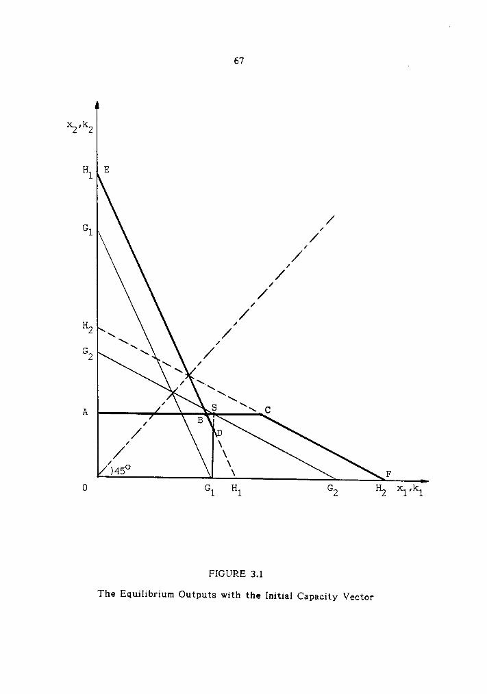
67 .

x2'k2

Hl E

/1Gl

/I

,//

1/

1

H’/

2 /1G /2

1

\\\\x

A S \ C

I

F

FIGURE 3.1

The Equilibrium Outputs with the Initial Capacity Vector

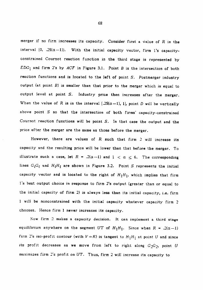
68

merger if no firm increases its capacity. Consider first a value of R in the

interval [0, .25(0.—1)). With the initial capacity vector, firm l’s capacity-

constrained Cournot reaction function in the third stage is represented by

EDG1 and firm2’s

by ACF in Figure 3.1. Point B is the intersection of both

reaction functions and is located to the left of point S. Postmerger industry

output (at point B) is smaller than that prior to the merger which is equal to

output level at point S. Industry price then increases after the merger.

When the value of R is in the interval [.2S(a—1), 1], point D will be vertically

above point S so that the intersection of both firms’ capacity-constrained

Cournot reaction functions will be point S. In that case the output and the

price after the merger are the same as those before the merger.

„ However, there are values of R such that firm 2 will increase its

capacity and the resulting price will be lower than that before the merger. To

illustrate such a case, let R - .2(c1.—1) and 1 < cz g 6. The corresponding

lines GiGi and HiHi are shown in Figure 3.2. Point S represents the initial

capacity vector and is located to the right of HIHI, which implies that firm

l’s best output choice in response to firm2’s

output (greater than or equal to

the initial capacity of firm 2) is always less than its initial capacity, i.e. firm

1 will be nonconstrained with the initial capacity whatever capacity firm 2

chooses. Hence firm 1 never increases its capacity.

Now firm 2 makes a capacity decision. It can implement a third stage

equilibrium anywhere on the segment UT of HIHI. Since when R - .2(¤.—l)

firm2’s

iso-profit contour (with V-}-R) is tangent to HIHI at point U and since

its profit decreases as we move from left to right along GQGQ, point U

maximizes firm2’s

profit on UT. Thus, firm 2 will increase its capacity to

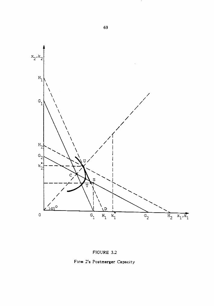
69

X2'H2

H1\\

/\ ,Gl \ //

X /\ /\ /\ /\\ /

\H\ /

2 \ / I/ IG2 \ / II \\U/IK

_.2 / \\ I

X \\'» S xLI \

\\\

x\\‘

\0 Gl Hl kl G2 H2 xl,kl

FIGURE 3.2

Firm2’s

Postmerger Capacity

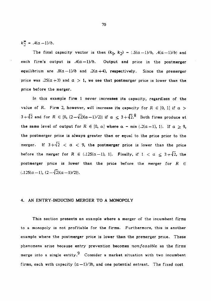
70

kt; - .40;;-1)/z>.

The final capacity vector is then (kl, kg) = (.5(a—1)/b, .4(0.—1)/b) and

' each firm’s output is .4(a—1)/b. Output and price in the postmerger '

equilibrium are .8(a—1)/b and .2(a—]-4), respectively. Since the premerger

price was .2S(a+3) and a > 1, we see that postmerger price is lower than the

price before the merger.

In this example firm 1 never increases its capacity, regardless of the

value of R. Firm 2, however, will increase its capacity for R E [0, 1] if 0. >

3+4-2 and for R E [0, (2—*l3)(0.—1)/2)) if 0, g 3-]-~l2.8 Both firms produce at

the same level of output for R E [0, on] where on - min (.2(a—1), 1). If cz 2 9,

the postmerger price is always greater than or equal to the price prior to the

merger. If 3+6 < G < 9, the postmerger price is lower than the price

before the merger for R E (.125(0.—1), 1]. Finally, if 1 < cz g 3-]-42, the

postmerger price is lower than the price before the merger for R E

(.1’.25(0.—l), (2—~l2)(a—1)/2)).

4. AN ENTRY-INDUCING MERGER TO A MONOPOLY

This section presents an example where a merger of the incumbent firms

to a monopoly is not profitable for the firms. Furthermore, this is another

example where the postmerger price is lower than the premerger price. These

phenomena arise because entry prevention becomes nonfeasible as the firms

merge into a single entity.9 Consider a market situation with two incumbent

firms, each with capacity (0.-1)/3b, and one potential entrant. The fixed cost

71

of the potential entrant is assumed to be 6+.03(o.—1)2/b with 6 > 0 very

small and let R — .2(a—1) (and thus V - .2(6—a)) with 1 < cz g 6.

As in Section 3, we start by examining whether the premerger market

situation is in equilibrium. We first show that the potential entrant decides

not to enter in the second stage of every premerger period given the

capacities of the incumbent firms.

As a preliminary step, suppose that each of the incumbent firms has

infinite capacity. They will be nonconstrained in the third stage whatever

capacity the entrant chooses in the second stage. Thus the equilibrium

output vector (in the third stage) is on the intersection of Cournot reaction

functions of the incumbent firms computed with V. If the entrant chooses a

capacity lc in the open interval (.3(ct—1)/b, oo), it is also nonconstrained and

the output levels of the firms are the same at .3(<1—l)/b. lf it chooses k: in

the interval [0, .3(¤.—1)/b], it is constrained and each of the incumbent firms

produces at the level of .4(a—1)/b — k/3. The maximum profit the potential

entrant can earn by entering is attained when it chooses a capacity of

.3(<1—1)/b. The corresponding output level of each incumbent firm is then

.3(0.-1)/b and the corresponding gross profit of the entrant is .O3(a—1)2/b.10

Return to the original potential entrant’s situation. It decides whether

or not to enter given that each incumbent firm has a capacity of (0.-1)/3b.

Suppose that it chooses a positive capacity. Depending on the entrant’s

capacity, the incumbent firms are either nonconstrained or constrained. As we

saw in the previous paragraph, the entrant’s profit—maximizing capacity, given

that the incumbent firms are nonconstrained, is .3(a—1)/b and its correspond-

ing gross profit is .03(¤.—1)2/b. We can easily compute its profit-maximizing

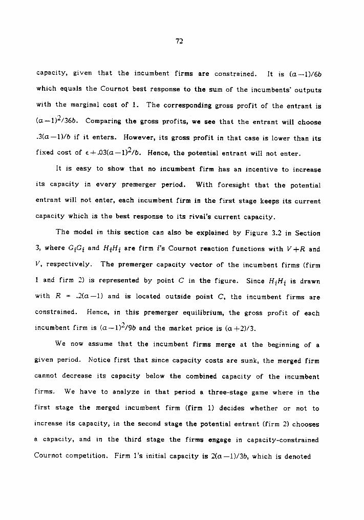
72

capacity, given that the incumbent firms are constrained. It is (a—l)/6b

which equals the Cournot best response to the sum of the incumbents’ outputs

with the marginal cost of 1. The corresponding gross profit of the entrant is

(c1.—l)2/36b. Comparing the gross profits, we see that the entrant will choose

.3(cz—l)/b if it enters. However, its gross profit in that case is lower than its

fixed cost of e+.03(a-I)2/b. Hence, the potential entrant will not enter.

It is easy to show that no incumbent firm has an incentive to increase

its capacity in every premerger period. With foresight that the potential

entrant will not enter, each incumbent firm in the first stage keeps its current

capacity which is the best response to its rival’s current capacity.

The model in this section can also be explained by Figure 3.2 in Section

3, where GiGi and HiI—Ii are firm i’s Cournot reaction functions with V-|—R and

V, respectively. The premerger capacity vector of the incumbent firms (firm

l and firm 2) is represented by point C in the figure. Since HiHi is drawn

with R == .2(o.—1) and is located outside point C, the incumbent firms are

constrained. Hence, in this premerger equilibrium, the gross profit of each

incumbent firm is (0.—1)2/9b and the market price is (0.+2)/3.

We now assume that the incumbent firms merge at the beginning of a

given period. Notice first that since capacity costs are sunk, the merged firm

cannot decrease its capacity below the combined capacity of the incumbent

firms. We have to analyze in that period a three-stage game where in the

first stage the merged incumbent firm (firm 1) decides whether or not to

increase its capacity, in the second stage the potential entrant (firm 2) chooses

a capacity, and in the third stage the firms engage in capacity-constrained

Cournot competition. Firm1’s

initial capacity is 2(u.—l)/3b, which is denoted

73

by k°l° in Figure 3.2. Since the equilibrium output vector in the third stage is

on UD (and it depends on firm 2’s capacity), firm 1 will always be noncon-

strained, even with its initial capacity. Thus firm 1 never increases its

capacity and if some output vector on UD yields a positive profit to firm 2,

firm 1 cannot prevent firm 2 from entering. As shown in Figure 3.2, the

output vector at point U gives firm 2 the maximum profit and firm2’s

gross

profit at that point is .08(a—1)2/b. Since the gross profit is greater than the

fixed cost, firm 2 enters with the capacity kg - .4(a—1)/b.

The final capacity vector in the postmerger and postentry equilibrium is

then (kl, kg) = (2(a——1)/3b, .4(a—1)/b) where each firm produces at the same

level of output .4(a—1)/b. The gross profit of the merged firm is then

2(a—1)(17——2cz)/75b. Since the premerger joint gross profits of the insiders

was 2(a—1)2/9b, even the merger to a monopoly hurts the participating firms

if 0. is greater than 76/31. The postmerger and postentry market price is

(0. +4)/5 and is lower than the premerger market price of (0. +2)/3.

Deneckere and Davidson (1985) argue that a merger to a monopoly is most

profitable but the free rider problem makes it less likely. However, in our

example, firms do not merge all the way to a monopoly, not because the free

rider problem prevents them from merging, but because the merger will cause

the potential entrant to enter and thus the insiders will be hurt seriously

from the merger. Our example provides a more plausible explanation for the

existence of an industry that is not a pure monopoly. lndeed, we believe that

one cannot properly assess the effects of a merger without taking into account

the possibility of entry.

74

5. CONCLUSIONS

The previous papers addressing the question of the incentives to merge

have never found that mergers can decrease industry prices, except Davidson

and Deneckere (1984) who have demonstrated in quantity-setting and price-

setting supergames that consumers can benefit from a merger. However, we

have shown in this chapter that mergers may decrease industry price. The

main reason for the result is that capacity costs for firms are sunk. Since

the merged firm cannot decrease its capacity below the combined capacity of

the insiders and thus is forced to commit to that capacity level, there are

situations where the outsiders increase their capacities much more than they

increase their outputs in a regular Cournot model.

We have also demonstrated that a merger to a monopoly is not always

beneficial, and this is a striking contrast to the results in the previous papers.

That is, there are situations, in our model, where if incumbent firms merge ·

into a single entity, entry prevention becomes impossible and allowing entry

hurts the insiders seriously.

We conclude that one cannot examine properly the effects of a merger

without considering the possibility of entry.

75

FOOTNOTES

1. The papers have another observation in common. They all conclude that

a merger never hurts the firms which are not participating in the merger.

We will discuss this outcome in Chapter IV.

2. There are many papers on strategic entry deterrence which introduce

sunk capacity costs as a credible entry deterrent (e.g., Dixit (1980),

Ware (1984)).

3. They also enumerate three potential problems with the quantity—setting

supergame analysis (see pp. 121-122).

4. We are in fact assuming that there is no potential entrant. In the rest

of this section we use "firm" instead of "incumbent firm".

5. Imagine the usual Cournot competition with either V or V4—R. The

best response of a firm to total output of the other firms for the former

is always greater than (if R > 0) or equal to that for the latter.

6. We assume an exogenous merger. Even though the postmerger price is

lower than the premerger price, the merger may be profitable to the

insiders since they can save fixed costs.

76

7. Since we assume that V+R = 1, we can interpret R as the proportion of

R to V-}-R.

8. If R = (2—~E)(a—1)/2, firm 2 is indifferent between increasing capacity

and staying put. We assume that in this case firm 2 stays put.

9. In our model, a merger of some incumbent firms typically makes

entry prevention nonfeasible.

10. We define gross profit = total revenue — (total cost — a fixed

cost).

CHAPTER IV

SUNK CAPACITY COSTS AND HORIZONTALMERGER WITH CAPACITY-CONSTRAINED

BERTRAND COMPETITION

1. INTRODUCTION

Several recent papers have investigated the issue of the existence of

incentives to merge. Davidson and Deneckere (1984), Perry and Porter (1985),

Salant, Switzer, and Reynolds (1983), and Szidarovszky and Yakowitz (1982)

have all demonstrated that mergers may reduce the joint profits of the

constituent firms (insiders) in quantity-setting games. On the other hand,

Davidson and Deneckere (1984) and Deneckere and Davidson (1985) have

observed that mergers are never disadvantageous in static price—setting games.

These studies, however, share the observation that the firms (outsiders)

which do not participate in a merger, benefit (or more accurately are never

hurt) from the merger. This observation is dated back to Stigler (1950).1

Davidson and Deneckere (1984) further show that in both the price-setting and

the quantity-setting supergames mergers in the industry with firms practicing

tacit collusion tend to be beneficial to the outsiders since the threat point

implicit in the collusion becomes more favorable for the outsiders.

In this chapter, adopting a model in which firms engage in capacity-

constrained price competition after they set capacities, we present an example

where a merger does hurt the outsiders.

77

78

We consider a market for a homogeneous product where capacity costs

are sunk in some appropriately defined time period once firms have installed

capacities. We assume that firms can immediately increase their capacities.

Starting with a premerger equilibrium in which no firm has an incentive to

increase its capacity, if some firms merge at the beginning of a certain period,

we have a three-stage game in the period. In the first stage, the merged firm

with the combined capacity of the insiders decides whether or not to increase

its capacity. In the second stage, after observing the capacity of the merged

firm, the outsiders choose their capacities simultaneously and independently.

To provide the advantage of being a first mover for the merged firm is

natural because the merged firm can commit itself to its postmerger capacity

before it announces the merger. In the third stage, after learning how much

capacity each firm has, the firms engage in capacity-constrained price

competition. We adopt the efficient·rationing rule. Our equilibrium concept

of the game is that of a subgame perfect Nash equilibrium.

In the example of Section 4, a merger hurts the outsider. Davidson and

Deneckere (1984) present a model very similar to ours. The reason why they

get a different result is that they do not consider the possibility that firms

increase their capacities after mergers. Indeed, in our example, both the

merged firm and the outsider increase their capacities.

Another interesting observation in the example is that the premerger

price is higher than the lowest price in the support of the postmerger (mixed

strategb') equilibrium. Interpreting mixed strategies as Edgeworth price cycles,

we may state that there are periods after the merger in which prices are

below the premerger price.2

79

Finally, we demonstrate in the example that unlike the previous static

price competition models, a merger reduces the joint profits of the partici-

pating firms. However, firms have incentives to merge because a merger

hurts the outsider more severely than the merged firm.

The chapter is divided into five parts. The basic model is presented in

the next section. In Section 3 we review and study further a duopoly with

capacity-constrained price competition. Section 4 contains an example which

carries out all the arguments. In Section 5 we present several conclusions.

2. THE MODEL

Consider a market for a homogeneous product with a linear demand. The

market demand function in each period is given by: D(1>) = a — p for 0 g p

g a and D(p) =- 0 for p > a, where D(p) is the quantity demanded at price p

and a is a positive constant. We assume that the production costs of a firm

in the industry depend on its installed capacity and a quasi-fixed cost (for

brevity, a fixed cost).3 Capacity and output are measured in the same units.

A firm with k units of capacity can produce up to k units of the product at

zero marginal cost. lf firm i has capacity ki and is producing output xi in a

given period, then its cost in that period is

Ci(xi, ki) - Fi —+- Rki for 0 < xi g ki

Rki for xi =· 0

80

where F.; is a fixed cost and R is a constant unit capacity cost. We assume

that capacity costs, once installed, are sunk but fixed costs are not. There is

no rental or resale market for idle capacity already in place. I-lence, over

time, each firm may increase but cannot reduce its capacity.

The demand function and the cost functions of firms in each period are

common knowledge to the firms. We assume that in each period firms engage

in price competition, subject to the capacity constraints chosen before the

stage of price competition when each firm learns how much capacity its

opponents have. We assume that each firm seeks to maximize its own

expected profit.

Consider a premerger equilibrium in which n competing firms have no

incentive to increase their capacities and there is no potential entrant. Now

consider a period where some firms merge. We then have a three-stage game

in that period. We treat the merged entity as a single firm whose initial

capacity is the sum of the capacities of the participating firms and whose

fixed cost is assumed to have a value between the smallest and the sum of

those of the insiders. In the first stage, the merged firm decides whether or

not to increase capacity above its initial level. In the second stage, after

observing the final capacity of the merged firm, the outsiders decide

simultaneously and independently whether or not to increase their capacities

above their premerger levels. In the third stage, after learning how much

capacity each firm has, the firms simultaneously and independently name

prices. We assume that all firms have perfect foresight about actions in the

following stages. Thus a relevant equilibrium concept for the three-stage

game is that of a subgame perfect Nash equilibrium.

81

We compare the premerger and the postmerger equilibria. In particular,

we examine the effects of the merger on industry prices and the profits of

the outsiders as well as the joint profits of the insiders.

In order to complete the description of the model, we have to elaborate

on our rationing rule. We adopt the rationing rule considered in Levitan and

Shubik (1972), Kreps and Scheinkman (1983), and Osborne and Pitchik (1986).4

We assume that consumers first seek to buy from the firms quoting the

lowest price. If the firms with the lowest price cannot satisfy the quantity

demanded at that price and if the quantity demanded at the next lowest price

is larger than total capacity of the firms with the lowest price, then the firms

naming the second lowest price sell their outputs to consumers. If the firms

with the second lowest price cannot satisfy the residual quantity demanded at

their price and if the quantity demanded at the third lowest price is larger

than total capacity of the firms with the first and the second lowest prices,

then unsatisfied consumers purchase from the firms choosing the third lowest

price, and so on. Assuming that income effects are absent, we have in each

"round” a residual demand function parallel to the market demand function.

Finally, if the residual quantity demanded at the price of a certain round can

be fully supplied and if there are more than one firm quoting that price, then

each of the firms sells a quantity equal to the residual quantity demanded at

the price multiplied by the proportion of its capacity to total capacity of the

firms.

82

3. DUOPOLY WITH CAPACITY—CONSTRAINED PRICE COMPETITION

The example we will present in the next section is of a duopoly in which

the merged firm and the outsider decide sequentially whether or not to

increase their capacities and then the two firms quote prices. Hence it is

helpful to study in this section a duopoly with capacity—constrained price

competition. We first discuss the pure strategy equilibrium or the support of

the mixed strategy equilibrium, and the corresponding expected revenue of

each firm, given their capacities, and then focus on their sequential capacity

choices.

There are two firms, firm 1 and firm 2. Their capacities are given by kl

and kg. We assume, for simplicity, that Fi - 0 and kl 2 kg > 0. Suppose

that the firms charge prices pi and pj in the interval [0, cz]. (When we use i

and j at the same time, we mean that j ;é i.) With our rationing rule

described in Section 2, the quantity sold by firm i is equal to min (kl, 0.-pi)

if pi<pj, min (ki, ki(a—pi)/k) if pi—pj, and min (ki, max (0, ¤.—kj—pi)) if

pZ>pj, where k = kl-}-kg.

It is straightforward to check that the (kl, kg) subgame has a unique

pure strategy equilibrium when (kl, kg) is in region I or IV of Figure 4.1.5

(The line AB can be interpreted as the usual Cournot reaction function of

firm 1 in the case of zero marginal cost.) In region I both firms name the

price of cz-kl-kg and in region IV each charges the price of zero.

We do not have a pure strategy equilibrium with (kl, kg) in regions II

and III.6 Let 4*j be a mixed strategy of firm j chosen from the set of

cumulative distribution functions on [0, 0.]. Then the expected revenue of

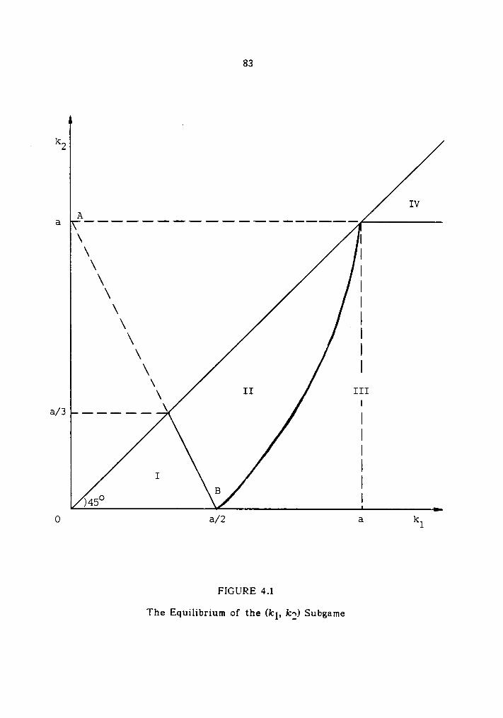
83

IVA

\ I\ II I\\ I

\ I\ I

x I\ I

I\\\ III

Ia/3 — — — — — \

I

III

IO a/2 a kl

FIGURE 4.1

The Equilibrium of the (kl, kg) Subgame

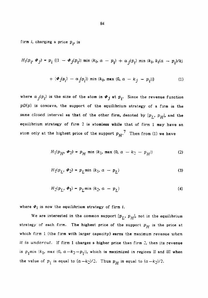
84

firm Z, charging a price pi, is

Hi(pi, <Pj) · pi {(1 — ¢j(pi)) min (ki, 0. — pi) -(- oLj(pi) min (ki, ki(a — pi)/k)

+ (¢_i(pi) — <xj(pi)) min (ki, max (0, G — kj — z¤i))} (1)

where ocj(pi) is the size of the atom in ¢j at pi. Since the revenue function

pD(I-1) is concave, the support of the equilibrium strategy of a firm is the

same closed interval as that of the other firm, denoted by [pi], pH], and the

equilibrium strategy of firm 2 is atomless while that of firm 1 may have an

atom only at the highest price of the support pH.7 Then from (1) we have

H1(DH, ¢'g) · DH min (ki, max (0, G — kg — 13H)) (2)

plimin(kl;Hg(PL,

4*1) · PLmi¤ (kg, G — LDL) (4)

where <Pi is now the equilibrium strategy of firm Z.

We are interested in the common support [pL, pH], not in the equilibrium

strategy of each firm. The highest price of the support pH is the price at

which firm 1 (the firm with larger capacity) earns the maximum revenue when

it is undercut. If firm 1 charges a higher price than firm 2, then its revenue

is plmin (kl, max (0, a—k:2—-p1)), which is maximized in regions II and III when

the value of pl is equal to (0.-kg)/2. Thus pH is equal to (cz —k2)/2.

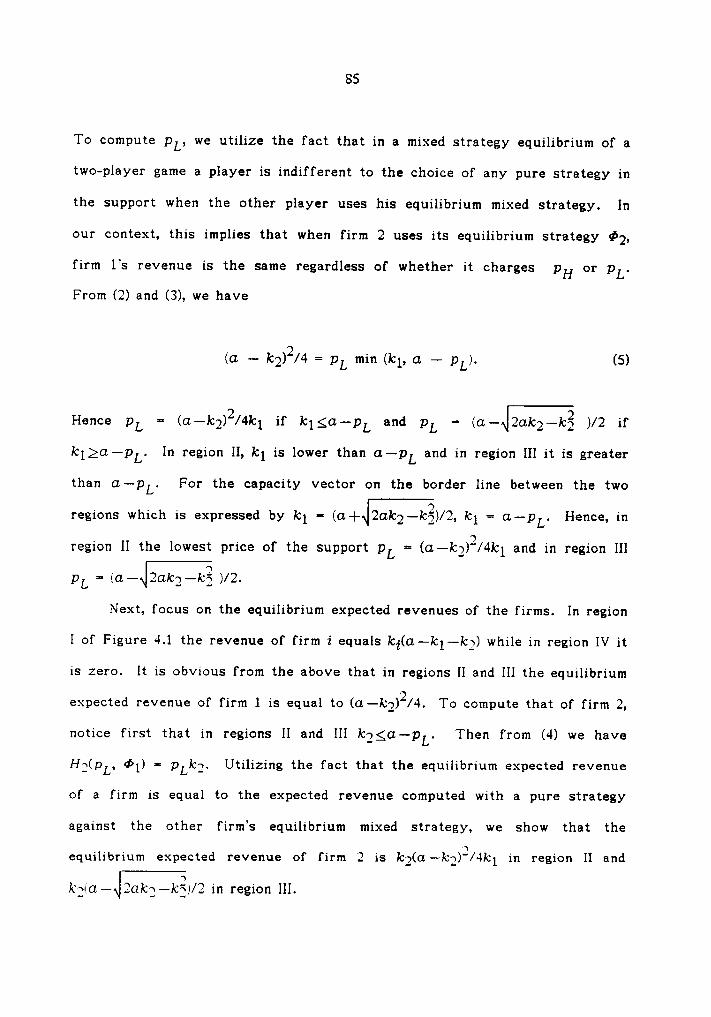
S5

To compute [JL, we utilize the fact that in a mixed strategy equilibrium of a

two-player game a player is indifferent to the choice of any pure strategy in

the support when the other player uses his equilibrium mixed strategy. In

our context, this implies that when firm 2 uses its equilibrium strategy ¢2,

firm1’s

revenue is the same regardless of whether it charges [JH or [JL.

From (2) and (3), we have

(ct — kg)2/4 = [JL min (kl, a — DL). (S)

Hence [DL = (cz—k2)2/4kl if kl ga—[JL and [JL =- (ci—(|2ak2—kä )/2 if

klga —pL. In region II, kl is lower than a—pL and in region III it is greater

than cz—[JL. For the capacity vector on the border line between the two

regions which is expressed by kl - (0.-}-(|20.k2—kg)/2, kl = 0.-pL. I-Ience, in

region Il the lowest price of the support pl! = (a—k_g)2/4kl and in region III

DLNext, focus on the equilibrium expected revenues of the firms. In region

I of Figure 4.1 the revenue of firm i equals ki(a —kl—k2) while in region IV it

is zero. It is obvious from the above that in regions II and III the equilibrium

expected revenue of firm 1 is equal to (0.—k2)2/4. To compute that of firm 2,

notice first that in regions II and III kjgcz-[JL. Then from (4) we have

Hj(pL, ¢l) = pLkg. Utilizing the fact that the equilibrium expected revenue

of a firm is equal to the expected revenue computed with a pure strategy

against the other firm’s equilibrium mixed strategy, we show that the

equilibrium expected revenue of firm 2 is k2(<1——kg)2/4kl in region II and

kg(c1.—„|2c1kj—kä)/2 in region Ill.

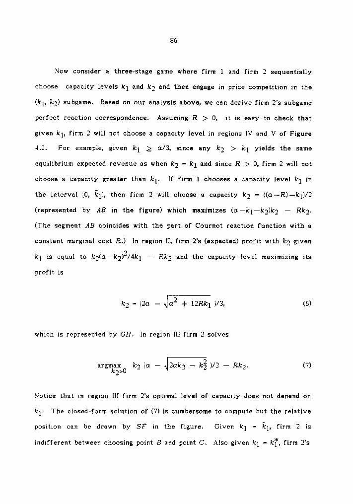
86

Now consider a three-stage game where firm 1 and firm 2 sequentially

choose capacity levels kl and kg and then engage in price competition in the

(kl, kg) subgame. Based on our analysis above, we can derive firm2’s

subgame

perfect reaction correspondence. Assuming R > 0, it is easy to check that

given kl, firm 2 will not choose a capacity level in regions IV and V of Figure

4.2. For example, given kl 2 cz/3, since any kg > kl yields the same

equilibrium expected revenue as when kg - kl and since R > 0, firm 2 will not

choose a capacity greater than kl. lf firm 1 chooses a capacity level kl in

the interval [0, kl), then firm 2 will choose a capacity kg — ((0.—R)—kl)/2

(represented by AB in the figure) which maximizes (a—kl—kg)kg — Rkg.

(The segment AB coincides with the part of Cournot reaction function with a

constant marginal cost R.) In region II, firm2’s

(expected) profit with kg given

kl is equal to kg(cL—kg)2/4kl — Rkg and the capacity level maximizing its

profit is

kg = (ZG — ylüg —l— 12Rkl )/3, (6)

which is represented by GH. In region III firm 2 solves

argmléi;0 kg (a — (|2cLkg — kg )/2 — Rkg. (7)

Notice that in region III firm2’s

optimal level of capacity does not depend on

kl. The closed—form solution of (7) is cumbersome to compute but the relative

position can be drawn by SF in the figure. Given kl - kl, firm 2 is

indifferent between choosing point B and point C. Also given kl =- kl, firm2’s

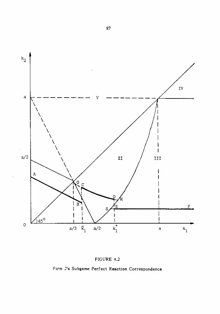
87

K2

IV

V\

I\ I‘I\

\ I\ I\ II I

\a/2 \ III\\ I. \ I

II I

I

I B I -I———-———I————FI FI I I I

0 I I45 IO ”

2 k* a k3/3 kl ä/ 1 1

FIGURE 4.2

Firm2’s

Subgame Perfect Reaction Correspondence

88

expected profit at point D is equal to that at point E. As a consequence, firm

2’ssubgame perfect correspondence comprises the union of [A, B], [C, D], and

[E, F]. Firm2’s

profit decreases as we move down from point A to point B

along the segment [A, B] and from point C to point D along [C, D], and is

constant on [E, F].

As a digression, we can transform our setting into a strategic entry

deterrence model. Let firm l be an incumbent and firm 2 a potential entrant.

Assuming that firm 2 enters if and only if it can earn a positive expected

profit, we first observe that preventing entry is not always feasible even with

Fg > 0. Given values of parameters F2 and R, if firm 2’s expected profit is

positive at the points on EF in Figure 4.2, it is impossible for firm 1 to deter

entry. A striking observation is that firm 1 can prevent entry with excess

capacity. That is, there are situations where firm 1 chooses a capacity level

greater than cz/2 (the output level maximizing a monopolist’s profit) and firm 2

decides not to enter, which implies that firm 1 has an lidle capacity in post-

entry periods. The main reason for this result is that in Figure 4.2 firm2’s

profit decreases as we move down from point C to point D along the segment

CD. This observation is a contrast to those in Dixit (1980), Ware (1984), and

others, who use quantity—setting models in which each firm’s marginal revenue

is always decreasing in the other’s output (i.e., the Cournot reaction function

of each firm is everywhere downward sloping).8

89

4. AN OUTSIDER-HURTING MERGER

We show in this section that a merger may hurt outsiders as well as

insiders and the postmerger prices may be lower than the premerger prices.

Consider a premerger market with three firms, each having the same fixed cost

F, and no potential entrant. Each firm has a capacity level of (0.-R)/4.

(Notice that the capacity is the same as a three~firm Cournot equilibrium

output with constant marginal cost R.) The parameters, 0., R>0, and F, have

values such that the firms make positive profits with their capacitites and

furthermore any firm’s predatory increase in capacity cannot succeed in

driving the rivals out of the industry. Under these conditions, it is easy to

check that the market is in equilibrium. That is, no firm has an incentive to

increase its capacity given the others’ capacities.

We have a unique pure strategy equilibrium in the price competition

subgame with these capacities. Each firm charges the price of (a+3R)/4 and

earns the profit of (O. —R)2/16 - F.9

Suppose now that two of the firms merge at the beginning of some

period. The initial capacity of the merged firm (called firm 1) is (0.-R)/2 and

that of the outsider (called firm 2) is (0.-R)/4. lf no firm increases its

capacity, postmerger prices are higher or equal to the premerger price. It is

immediate when a pure strategy equilibrium occurs in the (kl, kg) subgame

(region I in Figure 4.1). In the case of a mixed strategy equilibrium (region II

in Figure 4.1), the lowest price in the support pl! = (CL —kg)2/4kl > (614-3R)/4

(see Section 3). One can also verify with the explicit solutions in Section 3

that if both firms keep their initial capacity levels, they benefit from the

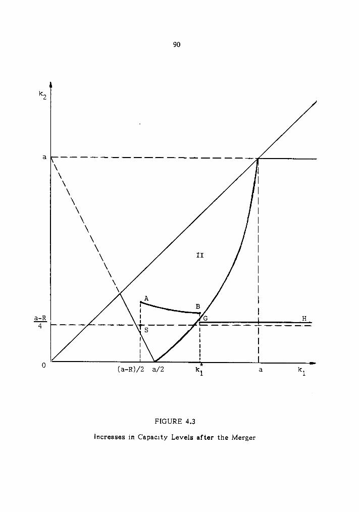
90

I‘I\

\ I\ I\ I\ I\ I\ I

I\\ H I\ II I\x I

A IIa-R I G I H

I I II II I II I

O (a-R)/2 a/2 kl a kl

FIGURE 4.3

Increases in Capacity Levels after the Merger

91

merger.

However, in our setting the firms may increase capacity above their

initial levels. Indeed, we are interested in such a case. We have in mind the

situation in Figure 4.3. The initial capacity vector is represented by point S.

Since the firms cannot decrease capacity levels (capacity costs are sunk), after

the first two stages in the period the final capacity vector is a point in the

union of [A, B] and [G, H], which are the parts of firm2’s

subgame perfect

reaction correspondence (see Figure 4.2). The exact location on the locus is

determined by firm1’s

capacity decision in the first stage. lf firm 1 stays

put at the initial capacity level, the final capacity vector is point A. If it

increases its capacity to kl, then the final capacity vector is either point B

or point G, etc. From the fact that firm 1’s equilibrium expected revenue is

(cz —kg)2/4 in region II and from expression (6), both studied in Section 3, we

have that firm1’s

expected profit along the segment [A, B] is

Ill -1 ¤, + .]¤2 + 12Rkl lg/36 - mel - 1-*. (8)

We can easily see that Hl is decreasing in kl. Hence, the only possible

position of the final capacity vector on [.4, B] is point .4. Next, firm1’s

expected profit along the segment [G, H] is also decreasing in kl. This is so

since while capacity costs are increasing in kl, its expected revenue is

constant throughout since along the segment its expected revenue is

(c1——Icg)2/4 and kg is constant. Thus point G is the only potential location for

the final capacity vector on the segment [G, H]. However, firm 2 is

indifferent between point B and point G when firm 1 chooses kl. To avoid

92

difficulties, we assume that firm 2 chooses point G in that case. Therefore,

to find the final capacity vector we only need to compare firm1’s

profits at

points A and G.

Since we do not have a closed-form solution for expression (7) in Section

3, we proceed by choosing particular values of the parameters. Let cz = 100, R

= 1, and F = 0. Then at point A firm1’s

capacity equals 49.5 and firm2’s

capacity is 32.3576 (computed from expression (6)). Firm1’s

expected profit at

this point is 1094.3731 (computed from expression (8)). Firm2’s

capacity at

point G solves for expression (7) with the values of the parameters and is

27.6410, and its profit is 400.4766. Since firm2’s

profit at point B is equal to

that at point G and by using expression (6) firm2’s

expected profit at point B

is expressed only with kl, we can get firm 1’s capacity at point G which is

85.5421. Then firm1’s

expected profit at point G is (¤.—kg)2/4 — Rkl =-=

1223.4124. With the values of the paramters, firm1’s

expected profit is

greater at point G than at point A. Hence, the final capacity vector is (kl, kg)

= (27.6410, 85.5421).

The premerger price is 25.75 and the range of postmerger prices is

{15.4885, 36.1795]. We may say that in some postmerger periods firms charge

prices below the premerger price. The profit of each firm before the merger

is 612.5625 while after the merger the expected profit of the merged firm is

1223.4124 and that of the outsider is 400.4766. The outsider’s profit is

lowered by 212.0859 while the joint profits of the insiders is lowered by only

1.7126.10 We cannot find the "free rider problem” discussed in some models of

a horizontal merger (e.g. Deneckere and Davidson (1985)). Rather, firms seek

to merge to avoid the disadvantage of being the outsider. Finally, we have

93

shown that the merged firm can get hurt from the merger even in a model of

price competition.

5. CONCLUSIONS

Previous papers focusing on an incentive to merge never found that

outsiders can suffer (profitwise) from mergers. Rather, they found that

outsiders benefit from mergers and thus each firm is better off waiting for its

rivals to merge. However, we have demonstrated in this chapter that a merger

can hurt outsiders more than insiders. In such a case the free rider problem

never occurs. We may expect that firms will either seek to merge or increase

capacities to make mergers unattractive.

In addition, we have shown that in a strategic entry deterrence model

where an incumbent and one potential entrant sequentially choose capacity

levels and then engage in capacity-constrained price competition, the incumbent

can prevent entry with excess capacity even in the case of a linear demand.

This observation is in contrast to those in Dixit (1980) and Ware (1984), while

Bulow, Geanakoplos, and Klemperer (1985) derived the same result.

94

FOOTNOTES

1. The papers share two other observations: (i) mergers, profitable or not,

always increase price(s) and (ii) a merger to a monopoly is always

profitable. We discussed them in Chaper III.

2. This observation is also a contrast to those in the previous papers.

For explanation about Edgeworth cycle, see Tirole (1988), p. 211, 234.

3. We assume, for simplicity, that each firm can produce up to its capacity

with zero marginal cost. We can generalize our arguments to the case of

a positive constant marginal cost by considering the price in the text as

the margin over the cost.

4. We adopt the efficient-rationing (parallel-rationing) rule for the analysis.

For explanation of another often considered rationing rule, called the

proportional—rationing (randomized—rationi¤§), see Davidson and Deneckere

(1986) or Tirole (1988), PD. 212-214.

S. The stage in which the two firms compete in prices, given their capacity

vector (kl, kg), is defined as the (kl, kg) subgame.

6. However, the mixed strategy equilibrium of the (kl, kg) subgame always

exists and is always unique. See Osborne and Pitchik (1986).

95

7. See Osborne and Pitchik (1986), PD. 244-245.

8. Bulow, Geanakoplos, and Klemperer (1985) demonstrate that the incumbent

may prevent entry with excess capacity even with a quantity-setting

model, if the Cournot reaction functions slope up.

9. See Brock and Scheinkman (1985), p. 373.

10. Notice that even with a small fixed cost the merger is profitable.

CHAPTER V

SUMMARY AND CONCLLJSIONS

We have examined the free rider problem of entry deterrence, the

profitability of a horizontal merger, and the effects of a horizontal merger on

the outsiders’ profits and industry prices, in markets where firms’ capacity

costs are sunk.

We have considered, in Chapter II, a three—stage entry deterrence model

in which in the first stage all incumbent firms facing a single potential entrant

choose their capacities simultaneously and independently, in the second stage

the potential entrant, after observing the incumbents’ capacity vector, chooses

its capacity, and in the third and final stage the firms engage in capacity-

constrained Cournot competition. Capacity costs are assumed to be sunk. If

the potential entrant enters the market (chooses a positive capacity), it must

sink in the second stage a fixed cost of entry as well as capacity costs.

Studying the subgame perfect Nash equilibria of the game, we have shown that

the free rider problem of entry deterrence can occur. That is, there are

situations where both entry prevention and allowing entry are equilibria but

entry prevention is mutually more profitable than allowing entry. This

observation is to be contrasted with that of Gilbert and Vives (1986). They

showed that the free rider problem never arises in a two-stage model which is

simply an extension of the Bain-Sylos—Modigliani limit pricing model to the

case of multiple incumbent firms.

96

97

One may argue that our observation about the free rider problem of

entry deterrence in our model is not significant and thus not interesting in

that if both entry prevention and allowing entry are equilibria and entry

prevention is mutually more profitable than allowing entry, then even

noncooperative incumbent firms will rather prevent entry. The criticism may

be overcome by modifying our model. Consider a three—stage game which is

the same as our model except that the incumbent firms are uncertain about

the cost of entry. We conjecture that there are situations where if the

incumbent firms could collude on their capacity decisions, entry prevention

would be optimal, but the unique subgame perfect equilibrium allows entry,

which implies that the free rider problem is significant. This conjecture is

based on two recent studies. Bernheim (1984) found the same phenomena as in

our original model but Waldman (1987a) demonstrated that in Bernheim’s model

the free rider problem of entry deterrence is significant if incumbent firms

are uncertain about the exact investment in entry deterrence needed to deter

entry. If our conjecture is correct, it is another contrast to Gilbert and

Vives's limit pricing model because Waldman (1987a) observed that in Gilbert

and Vives”s model there is no evidence of underinvestment in entry deterrence

even if the incumbent firms are uncertain about the fixed cost of entry.

In Chapter ll we have also shown the following. Increasing the number

of incumbent firms may cause the equilibrium price to increase and thus

consumer welfare to decrease. In all subgame perfect equilibria no firm has

excess capacity. There may exist a continuum of entry—allowing equilibria and

the total equilibrium output may be different across the equilibria. A

decrease in the cost of entry may increase the equilibrium price and hurt

98

consumers. A decrease in demand may result in an increase in total output.

Modifying the original model into a model with multiple potential entrants

which choose capacities sequentially, we have established that whenever

preventing entry is feasible, there is an entry-preventing equilibrium. We

have also demonstrated that even with multiple potential entrants the free

rider problem of entry deterrence can occur.

Several recent papers which theoretically analyze the profitability of a

horizontal merger and its effects on the outsiders’ profits and industry prices,

all observed that a merger never decreases industry prices, a merger to a

monopoly is always profitable, and a merger never hurts the outsiders.

However, we have shown that these observations can be reversed even in the

models which are prevalent in the industrial organization literature.

Considering a market for a homogeneous product where firms with sunk

capacities compete in quantities and there are potential entrants, we have

illustrated in Chapter III that a merger may decrease industry price and a

merger to a monopoly is not always profitable. The latter observation is

striking because no previous study explained explicitly the real life

observation of the existence of an industry that is not a pure monopoly. In

our model, firms may not merge all the way to a monopoly because then they

cannot prevent entry. Indeed, we believe that in order to properly assess the

effects of a horizontal merger, the possibility of entry should be taken into

consideration.

In Chapter IV we have considered a market for a homogeneous product in

which firms with sunk capacities engage in capacity-constrained price

competition and presented an example where a merger hurts the outsider.

99

Another interseting observation in that example is that the premerger price is

higher than the lowest price in the support of the postmerger mixed strategy

price equilibrium. Interpreting mixed strategies as Edgeworth price cycles, we

may say that there are periods after the merger in which prices are below the

premerger price. We have also demonstrated in the example that unlike the

previous static price competition models, a merger reduces the joint profits of

the participating firms. In the example firms still have incentives to merge

because a merger hurts the outsider more severely than the merged firm,

which differs from the previous studies.

We have also shown in Chapter IV that excess capacity can prevent

entry in a model where an incumbent and one potential entrant sequentially

choose capacity levels and then engage in capacity-constrained price

competition.

BIBLIOGRAPHY

Allen, B., "Capacity Precommitment as an Entry Barrier for Price Setting

Firms," CARESS Working Paper # 85-33, University of Pennsylvania,

November 1986.

Bain, J.S., Barriers to New Competition, Cambridge: Harvard University

Press, 1956. ·

Bernheim, B.D., "Strategic Deterrence of Sequential Entry into an Industry,”

Rand Journal of Economics, Vol. 15 (1984), pp. 1-11.

Bernheim, B.D., Peleg, B., and Whinston, M.D., "Coalition-Proof Nash Equilibria

I. Concepts," Journal of Economic Theory, Vol. 42 (1987), PP. 1-12.

Bulow, J., Geanakoplos, J., and Klemperer, P., "Holding Idle Capacity to Deter

Entry," Economic Journal, Vol. 95 (1985), PD. 178-182.

Brock, W.A. and Scheinkman, J.A., "Price Setting Supergames with Capacity

Constraints," Review of Economic Studies, Vol. S2 (1985), pp. 371-382.

Davidson, C. and Deneckere, R., "Horizontal Mergers and Collusive Behavior,"

International Journal of Industrial Organization, Vol. 2 (1984),

pp. 117-132.

Davidson, C. and Deneckere, R., "Long-Run Competition in Capacity, Short-Run

Competition in Price, and the Cournot Model," Rand Journal of

Economics, Vol. 17 (1986), pp. 404-415.

Deneckere, R. and Davidson, C., "Incentives to Form Coalitions with Bertrand

Competition," Rand Journal of Economics, Vol. 16 (1985), PD. 473-486.

100

101

Dixit, A.K., "A Model of Duopoly Suggesting a Theory of Entry Barriers,” Bell

Journal of Economics, Vol. 10 (1979), pp. 20-32.

Dixit, A.K., "The Role of Investment in Entry·Deterrence," Economic

Journal, Vol. 90 (1980), pp. 95-106.

Eaton, B.C. and Ware, R., "A Theory of Market Structure with Sequential

Entry," Rand Journal of Economics, Vol. 18 (1987), pp. 1-16.

Fudenberg, D. and Tirole, J., "Capital as a Commitment: Strategic Investment to

Deter Mobility/’ Journal of Economic Theory, Vol. 31 (1983),

pp. 227-250.

Gilbert, R.J., "Preemptive Competition,” in J.E. Stiglitz and G.F. Mathewson,

eds., New Developments in the Analysis of Market Structure,

Cambridge: MIT Press, 1986, pp. 90-123.

/GiIbert, R.J., “Mobility Barriers and the Value of Incumbency," in

R. Schmalensee and R. Willig, eds., Handbook of Industrial

Organization, forthcoming, mimeo, May 1987.

Gilbert, R..I. and Vives, X., "Entry Deterrence and the Free Rider Problem,"

Review of Economic Studies, Vol. 53 (1986), pp. 71-83.

Harrington, .I.E., Jr., "Oligopolistic'Entry Deterrence under Incomplete

Information/’ Rand Journal of Economics, Vol. 18 (1987), pp. 211-231.

Kreps, D.M. and Scheinkman, J.A., "Quantity Precommitment and Bertrand

Competition Yield Cournot Outcomes,” Bell Journal of Economics,

Vol. 14 (1983), pp. 326-337.

Kreps, D.M. and Wilson, R., "Reputation and Imperfect Information,” Journal

of Economic Theory, Vol. 27 (1982), pp. 253-279.

102

Levitan, R. and Shubik, M., "Price Duopoly and Capacity Constraints,"

International Economic Review, Vol. 13 (1972), Pp. 111-122.

McLean, R.P. and Riordan, M.I-I., “Industry Structure with Sequential

Technology Choice,” Journal of Economic Theory, Vol. 47 (1989),

pp. 1-21.

Milgrom, P. and Roberts, J., "Limit Pricing and Entry under Incomplete

Information: An Equilibrium Analysis," Econometrica, Vol. 50 (1982),

pp. 443-460.

Osborne, M.J. and Pitchik, C., "Price Competition in a Capacity-Constrained

Duopoly,” Journal of Economic Theory, Vol. 38 (1986), pp. 238-260.

Perry, M.K. and Porter, R.H., "Oligopo1y and the Incentive for Horizontal

Mergex·,” American Economic Review, Vol.75 (1985), pp. 219-227.

Prescott, E.C. and Visscher, M., "Sequential Location among Firms with

Foresight," Bell Journal of Economics, Vol. 8 (1977), pp. 378-393.J

Salant, S.W., Switzer, S., and Reynolds, R.J., "Losses from Horizontal Merger:

The Effects of an Exogenous Change in Industry Structure on Cournot-

Nash Equilibrium,” Quarterly Journal of Economics, Vol. 98 (1983),

pp. 185-199.

Salop, S.C., "Strategic Entry Deterrence,” American Economic Review,

Vol. 69 (1979), pp. 335-338.

Schmalensee, R., "Economies of Scale and Barriers to Entry," Journal of

Political Economy, Vol. 89 (1981), pp. 1228-1238.

Spence, A.M., "Entry, Capacity, Investment and Oligopolistic Pricing,"

Bell Journal of Economics, Vol. 8 (1977), PD- 534-544.

103

Spulber, D.F., "Capacity, Output, and Sequential Entry," American Economic

Riview, Vol. 71 (1981), pp. 503-514.

Stigler, GJ., “Monopoly and Oligopoly by Merger," American Economic

Review, Vol. 40 (1950), pp. 23-34.

Szidarovszky, F. and Yakowitz, S., "Contributions to Cournot Oligopoly

Theory,” Journal of Economic Theory, Vol. 28 (1982), pp. 51-70.

Tirole, J., The Theory of Industrial Organization, Cambridge: MIT press,

1988.

Vives, X., “Sequentia1 Entry, Industry Structure, and Welfare," European

Economic Review, Vol. 32 (1988), PP- 1671-1687.

M//Waldman, M., "Noncooperative Entry Deterrence, Uncertainty, and the Free

Rider Prob1em," Review of Economic Studies, Vol. 54 (1987a),

‘ pp. 301-310.

Ä/aldman, M., "Underinvestment in Entry Deterrence: When and Why,"

UCLA Working Paper No. 456, October 1987b.

Ware, R., "Sunk Costs and Strategic Commitment: A Proposed Three-Stage

Equi1ibrium," Economic Journal, Vol. 94 (1984), pp. 370-378.

APPENDICES

104

105

APPENDIX A

This appendix provides proofs of lemmas in Section 3 of Chapter II.

Proof of Lemma 4. Proof of part (c). We show that D(km+1) Q D(km+1).

Suppose i§£D(km+l). Then D(km+l)- D(km+1), since it follows from part (b)

that the equilibrium outputs of each firm are the same in the two subgames.

Consider the case where i€D(km+1). Let firm j be a firm which has the

largest capacity among the firms in D(km+1)\{i). If it does not exist, then we

are done. In the case where it does exist, we are only required to show that

„iED(km+l) by Lemma 3 (c). On the contrary, suppose thatj§ED(km+1).

Then

ki =

kiFirst,we show that §h(km+1) >xh(km+1) for all h€Ü\{i}\D(km+1). By

Lemma 3 (e), :T:h(km+l) > §i(km+1). Since :T:j(km+1) is equal to ki, the capacity

of firm h is larger than that of firm j, kh > ki. It implies with _j6£D(km+l)

thath<ZD(km+1)

(see Lemma 3 (c)). Since both firms h and j are not strictly

constrained, we get xh(km+1) = xi(km+l) by Lemma 3 (d). I—Ience xh(km+1)

2 2_i<1'i"‘+1> = 2hc12"‘+1).Second, §h(km+1) 2

äh(km+1) for all hED(k"‘+1)\{i}, since firm h is

strictly constrained in the km"'1 subgame and its capacities are the same in the

two subgames.

Third, we show that ?<i(km+1) >xi(km+l).

Suppose that iEL(km+1).

Then :?i(km+1) = ki. We get§i(km+1)

= ki from the hypothesis that

106

iED(km+l). Since ki > ki, we are done. Suppose next that i&’L(km+1). Then

since firm_j is strictly constrained and firm i is nonconstrained in the

k"‘+1

subgame, we have xi(km+1) > :'Ei(km+1)- ki by Lemma 3 (e). We also have ki

= ki 2 k_i<k"‘+l) > ki(1E’“+1). it rauaws from the rack um_1e1>(k“‘+1)

buti€D(km+1), and from Lemma 3 (e). Both relations yield §i(km+1) > §i(km-H).

Hence from the three results above we have Y-i(km+1) >§-j(km+1),

which implies with Lemma l (a) that t(Y-j(km+1)) g t(Y-i(km+1)). This leads to

a contradiction.

We can show L(km+1) Q L(km+1) by arguments similar to those of the

first part. Q.E.D.

Proof of part (d). By Lemma 3 (d), §i(km+1)-

ij(km+1) = x(km+1) and xi(km+1)

= :?:‘i(km+1) = §(km+1) for i, _jE l7l\L. Let h be the cardinality of Ü\L. Then

k<1E"‘+1) = zajiaiki + (h——1)§(km+1)), k<km+1) = iigiiiki + <1«—i)k<km+1)),Y(km+1) = Eijsilli +

h§(km+1), and Y(km+1) = E-jgiiki —+— h§(km+1). Since

firm i belongs to L, to complete the proof we need only to show that i(z) =

t(z—i—(h—1)§(z)) is decreasing in z and )x;(z)· z -i— h§(z) is increasing in z

where z is a variable between Zjai-{ki and Ejsi-ki. lndeed, d§(z)/dz -t’(·)/ll—t’(·)(h—1)] < 0 and dIT(z)/dz = 1 -i- ht’(-)/[1—t’(·)(h—1)] > 0.

Q.E.D.

Proof of part (e). Since i€D(km+1), it follows from part (a) that there exists

iii > ki such um kieD(kf‘Q+1, ki) but kieiikyl, ki). Let k;" be mm (ki, ki).

Then §(km+1) E §(k?;+l, ki) =j€(k3+1,

k;°°). Notice that when ki > käk = ki,

the equality comes from the fact in part (b). Hence, we need only to show

107

thatln

the first step, choose ki E (ki, ki°‘] such that it is the largest capacity

of firm i satisfying D(km+1) = L(km+l\k}). It is possible from the facts in

part (c). If ki < ki°‘, then in the second step choose kg E (ki, ki°°] such that

it is the largest capacity of firm i satisfying D(k?i+1, ki) = L(k?i+1, k?).

Repeat steps until kik is chosen. It follows from part (d) that at each step the

total output increases.

Hence >?c1E{‘§+1, uf) > >?c12"‘+l>. Q.E.¤.

Proof of Lemma 5. It is obvious that firm m+1 is constrained in the km+1

subgame. lt follows from the fact that t(2i£M ki) 2 r(2i:M ki) - km.i,i (see

Lemma 1 (c)), and from Lemma 3 (f).

Second, we show that firms with the same capacities in the two subgames

are constrained in the km+1 subgame. Let firm i be a firm with ki - ki where

iEM. Then we have Eid]-ikii > Ejaüiiki. It follows from the fact that

the total capacity in the km+1 subgame is larger than that in thekm-,-1

subgame (see Lemma 1 (b)) and from the fact that ki - ki. We also have

from the fact that all firms are constrained in

the km+1 subgame. Now we are prepared to shgw ki

Swhichmeans that i6L(km+1). Indeed, ki — ki S t(Zj_M §ii(km'*'1)) =° -iThe first inequality comes

from the hypothesis that firm i is constrained in the km+1 subgame and the

last one follows from the fact that the output of each firm cannot exceed its

capacity and from Lemma 1 (a).

Finally, we show that iEL(km+1)for iEM with ki > ki. Suppose first

108

that EFM-iki g Zjsi-Liki. Then Lemma 1 (a) implies that 2t(2iSi\-Tiiiki). Next since all firms are constrained in the km+1 subgame, wehave ki g t(Ej€M_i§i(km+1)) =· t(ZjSi\-iiiki). Thus we derive the following: ki

< t(Zi€i-i-i ki) g Kzjzüii >T:i(km+1)), which means that iEL(km-H). Consider

the case where EFM-iki > Ejsi-1-iki.From the fact that the total capacity

ln thek“‘+1

subgame ls larger than that in the subgame, we get

Zjsii-I-iki - ZJEM-iki < ki- ki. Then by Lemma 1 (b) we have t(2j8i-iiiki)— MZJSM-iki) < ki - ki. Since ki g t(Ei€i-i-ikii), we obtain ki <

t(ZiSii-iii

ki)Proofof Lemma 6. Since firm i is constrained in the km+1 subgame, we have

t(Y_i(km+1)) 2 ki. We also have t(Y_i(km+1)) < ki from the hypothesis that

firm i is nonconstrained in thekm+1

subgame. Together with ki 2 ki, they

yield t(Y_i(km+1)) > t(i_i(km+l)). Then it implies with Lemma 1 (a) that

§_i<km+li S ii ck"‘+1>. henee i(k“‘+1> = ?_i<km+1> + ki S §_ickm+1> +t(]T{_i(km+1)) <

]k_i(km+1)+ t()?_i(km+1) ) -

~)k(km+1). The strict inequality

results from Lemma 1 (b). Q.E.D.

Proof of Lemma 7. Suppose on the contrary that there exists firm i, for i·EM,l

which is nonconstrained in thekm+1

subgame. Then since it is constrained in

thek*“+l

eebgeme and nonconstraincd in thek’“+l

subgamc and since ki 2 ki,

it follows from Lemma 6 that Y(km+1) <)T(km+1), which contradicts the

hypothesis

thatProofof Lemma 8. Let km.i,i be a capacity in A(km) which firm m+1 chooses

109

in the km subgame. In the case where it is zero, the proof is trivial.

Consider the case where km.,} > 0. We must show that firm m+1 is

constrained. Suppose on the contrary that it is nonconstrained. Then there

exists a km.,}> 0 such that l”I(km, km.,}) > H(km, km.,}), which contradicts the

hypothesis that km.,}€A(km). Indeed, let 12m+l -§m.,}(km, km.,}). Then 12m+l

< km.,} and firm m+1 is not strictly constrained in the (km, km.,}) subgame.

Thus by Lemma 4 (b) we get §i(km, km.,}) — §i(km, km.,}) for all iEM, which

implies with R > 0 and Em+1 < km.,} that l'l(km, km,}) > l'l(km, km.,}).

Q.E.D.

Proof of Lemma 10. We first show that in thekm

subgame any capacity of

firm m+1, km.,}, such that iEL(km, km.,}) for some DEM, cannot be an element

of A(km). By Lemma 8, if m+1+T£L(km, km.,}), then km.,}i£A(km). Suppose next

that there exists a 12m+l such that m+1EL(km, km.,}) but i%L(km, km.,}) for

some i€M. Then km.,} > km.,} (see Lemma 4 (c))andby

Lemma 6. Let km.,} satisfy IT(km, km.,}) -Ükm, km.,}) and

m+l€L(km, km.,}). Such a km.,} exists since Y(km+1) <Ükm, km.,}) g

Ükm, km,}) (see Lemma 4 (e)) and ITL) is continuous in km.,} (see Lemma 3 (a)).

Notice that km.,} 2 km.,} and km.,} — km.,} g 2iEM(ki — ki). Let km.,} be

such that km.,}) = Y(km+1). Then m+1EL(I2m, km.,}) since km.,} > km.,}

(see Lemma 4 (e)) and m+1€L(km, km.,}). And by Lemma 7, M CL(km,

km.,}).

We are prepared to show that H(km, km.,}) > [I(km, km.,}), which implies

km.,}—EA(km). The profit of firm m+1 with km.,} is lI(km, km.,}) =

km+}[f(Y(km+1))—V—R] - F = n<1im+1> + 1r(x<km+1>>—v—R1<1i;;,,}—km,}> and

um with im.,} is nnlm, 12,,,,,) - 12„,+,1r<m"‘, k;,,„.,>>—v—R 1 — F -

110

H(km,kim,i) + [(f(Y(km, From the fact that

kim.iEA(km), we have II(km+l) 2 II(km, We also get

> [f(§(km, sinceY(km,

kim.l) > I?(km+1) and l<;i+1 —kim.i - EÜM (ki — ki ) 2 kim.} ·—

k;m.i. Both facts yield the inequality we want to establish.

We have shown that A(km) contains only a capacity (or capacities), kim,i,satisfying L(km,

kim.i) - Ni. Notice then that H(km+1)> I'I(km, kim.i) for all

l2m+1 > 0 such that 12m+l ¢ §m+1 and L(km,kim.i) = Ü. lt follows from the

fact that Lemma 5 implies L(km+1)- Ü, and from the fact that kim.i =

r(Zi€M ki). l-lence we have the following: if km+i > 0, then ki.m,i -

kimi) and thus A(km)-

{kriimi};if im+1 = 0, then

argé11nai<1>0lI(k , kim,i) does not exist and thus A(k ) - { 0 }. Q.E.D.

Proof of Lemma 11. We first show that in the (Y/m)m subgame, any positive

capacity of firm m+1 ends up with nonpositive profit to the firm and thus

kim.i - 0. By Lemma 3 (b), for any kim,.i > 0, we have §i((Y/m)m, kim,i) -§((Y/m)m, kim,i) for all

i€M.Suppose that kim,i > 0 satisfies

§((Y/m)m, kim,i) < Y/m. That is, i<;‘£L((Y/m)m, kim,i) for all iEM. Then since

kim.i) and x((Y/m)m, kim,i)— §(kg‘,

kim.i) (see

Lemma 4 (b)), l'l((Y/m)m, kim.i) - H(k„T, kim,1) g E(k„T) g 0. Suppose next that

kim,1 > 0 satisfies §((Y/m)m, l<i.m.i) — Y/m. Then the total output of

incumbent firms is just the limit output Y and thus ll( (Y/m)m, kim.i) g 0.

We now show that L((Y/m)m, 0) - l7i. Trivially, firm m+1 is constrained.

We must show that all incumbent firms are constrained. Suppose on the

contrary that §((Y/m)m, 0) < Y/m. Then there exists kim,i > 0 such that

111

Il((Y/m)m, k,,,+i) > 0. Indeed, let k,,,+i =- r(Y). In the ((Y/m)m, r(Y)) subgame

firm m+1 is constrained by Lemma 3 (f) but all incumbent firms are noncon-

strained by Lemma 4 (c). We have then m§((Y/m)m, r(Y)) < Y. Thus the

profit of firm m+1, l”I((Y/m)m, r(Y)), is greater than zero:

r(Y)[f(m§((Y/m)m, r(Y))+r(Y))—V—R] — F > r(Y)[f(Y+r(Y))——V—·R] — F - 0.

Since all incumbent firms are nonconstrained in the ((Y/m)m, r(Y)) subgame,

Lemma 4 (b) implies )T(k,T, r(Y) ) - Y((Y/m)m, r(Y)). Hence H(k.T, r(Y)) -

1'I((Y/m)m, r(Y)) > 0, which contradicts the hypothesis that E(k.T) S 0.

Q.E.D.

Proof of Lemma 12. Let k,,,+i = r(2iSM ki ) - r(Y). We first show that

L(km+l) =- 17I. From Lemma 3 (f) it follows that firm m+1 is constrained.

Suppose on the contary that i€:’L(km+1) for some iEM. Then ZJSM§‘i(km+l)

< Y implies l”I(km+1) = — F >

k,,,.,.i[f(Y—1—k,,,+i)——V—R ] — F = 0. This contradicts the hypothesis that firm

m+1 stays out in the equilibrium of the km subgame.

Next we show that k,,,+i~€A(km). Suppose that 1-;,,,+i+ZA(km). Then there

should exist 12,,,+, > 0 such that nikm, 12,,,+1) > n<km+1> = 0. This againleads to a contradiction to the hypothesis that 1;,,,+1 - 0 in the km subgame.

Then we haveA(km)

= {r(Z,€M ki)). It follows from the fact that

L(km+1) = N1 and l<,,,+iE A(km), and from Lemma 10.

1—lence E(km) > 0 and A(km) = {r(Zi£M ki)) imply that in thekm

subgame, ki). The fact that all firms are constrained in the

equilibrium of thekm

subgame comes from the results above and from

Lemma 5. Q.E.D.

112

APPENDIX B

This appendix provides subgame perfect equilibria for different values

of F and Q in the case of a single incumbent firm. The incumbent firm is

called firm 1 and a potential entrant is called firm 2.

(1) Compute first E(k}.,).

(1) If 0 < Q g (a—l)/S, then E(k.l.) ·(a—1—-2Q)(a+Q——l)/9b — F.

(ii) If(a—1)/5 g Q < min (a—l, 1) or Q -1 with 2 < a g 6,

then E(k.}..) = (a—Q—l)2/8b — F.

(111) If a—l g Q gl with 1 < a g 2, then E(k}.) < 0.

(2) Subgame perfect equilibria in the case of E(k}.) > 0.

(1) If O < Q g(a—1)/S, then kl -kE

· (a—l)/b —

2„|(a—1—2Q)(a+Q—1)/3b and k2 - kg = «l(a—1-—2Q)(a+Q—l)/3b.

(ii) If (a—l)/5 g Q g (2—~l-2)(a—l)/2, then k1= kE= (a—l)/b —

J5(a—a-1)/2b and k2 - kg - NE (a—Q—1)/4b.

(iii) If (2—«l2)(a—1)/2 g Q < min (a—l, 1) or Q - 1 with 2 < a g 3-{-J2,

then kl -ks —(a—1)/2b and k2 - kä—(a—1)/4b.

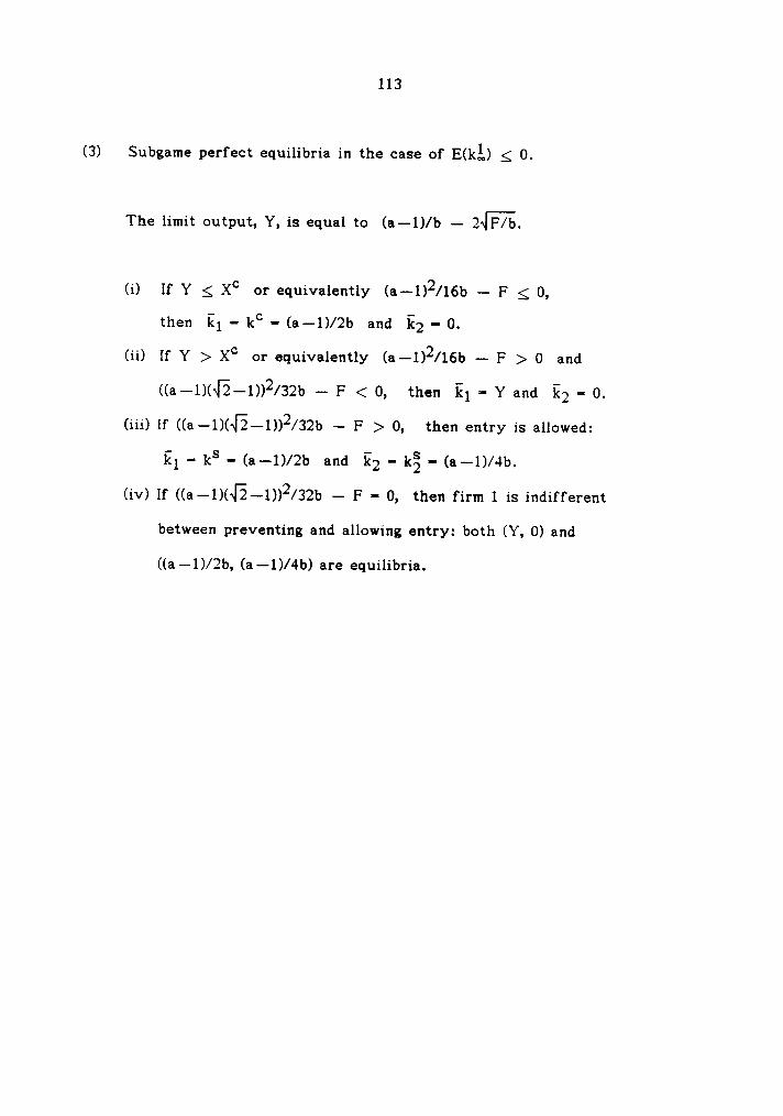
113

(3) Subgame perfect equilibria in the case of E(k}„) g 0.

The limit output, Y, is equal to (a—1)/b — 2«l F/b.

(i) If Y g XC or equivalently (a—1)2/16b — F g 0,

then E1 -kc

- (a—l)/2b and E2 - 0.

(ii) If Y >XC or equivalently (a—1)2/16b —- F > 0 and

((a—l)(~E—l))2/32b —- F < 0, then 1-E1 - Y and E2 = 0.

(iii) lf ((a—l)(Ö—1))2/32b — F > 0, then entry is allowed:

121 -ks

- ta-1)/26 and E2 - kä - (a—l)/4b.(iv) If ((a—1)(~l5—1))2/32b — F - 0, then firm 1 is indifferent

between preventing and allowing entry: both (Y, 0) and

((a—l)/2b, (a—1)/4b) are equilibria.

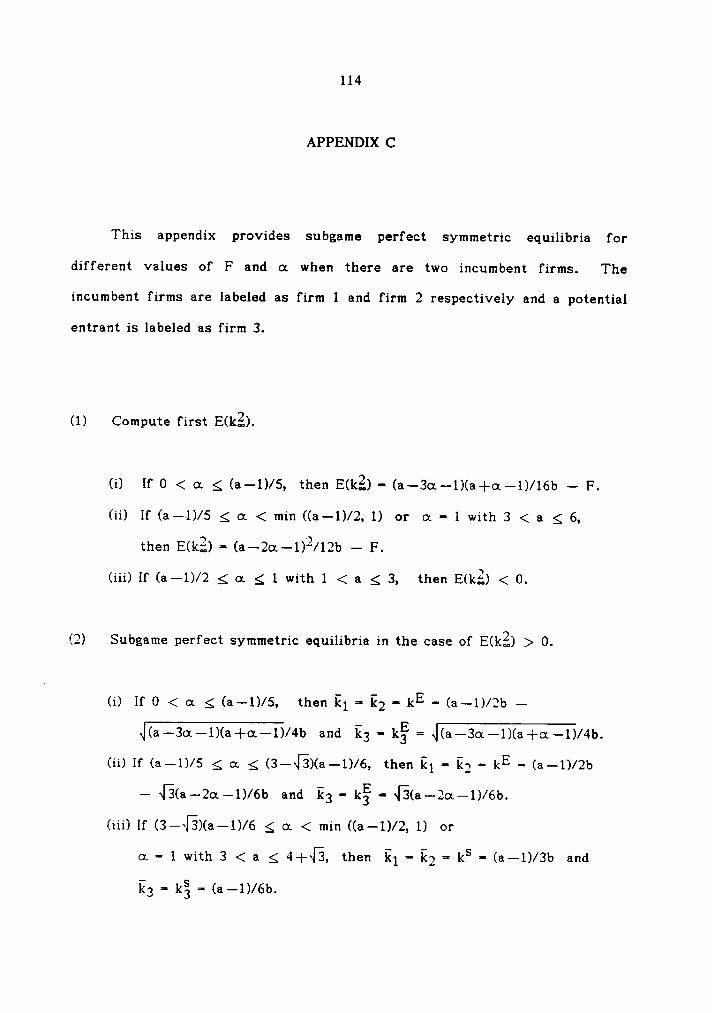
114

APPENDIX C

This appendix provides subgame perfect symmetric equilibria for

different values of F and on when there are two incumbent firms. The

incumbent firms are labeled as firm 1 and firm 2 respectively and a potential

entrant is labeled as firm 3.

(1) Compute first E(k?,).

(i) If 0 < ot g (a—1)/5, then E(k?.)-(a—3ot—1)(a+ot-1)/16b —- F.

(ii) If (a—1)/5 g ot < min ((a—1)/2, 1) or cx = 1 with 3 < a g 6,

then E(k„;.) = (a—2ot—1)2/12b — F.

(iii) If (a—1)/2 g ot g 1 with 1 < a g 3, then E(k§.) < 0.

(2) Subgame perfect symmetric equilibria in the case of E(k;2.) > 0.

(i) If 0 < ot g (a—1)/5, then kl = kg -kE

- (a—1)/2b —

„|(a —3c1—1)(a+<x—1)/4b and E3 - kg = „|(a—3ot—1)(a+on—1)/4b.

(ii) lf (a—1)/5 g ot g (3—~(3)(a—1)/6, then kl = kg = kE = (a—1)/2b

— x|3(a——2oL—1)/6b and kg = kg - ~13(a—2ot—1)/6b.

(iii) If (3—~[3)(a—1)/6 g ot < min ((a—1)/2, 1) or

ot = 1 with 3 < a g 4-ME, then kl - kg = ks- (a—1)/3b and

kg - kg - (a—1)/6b.

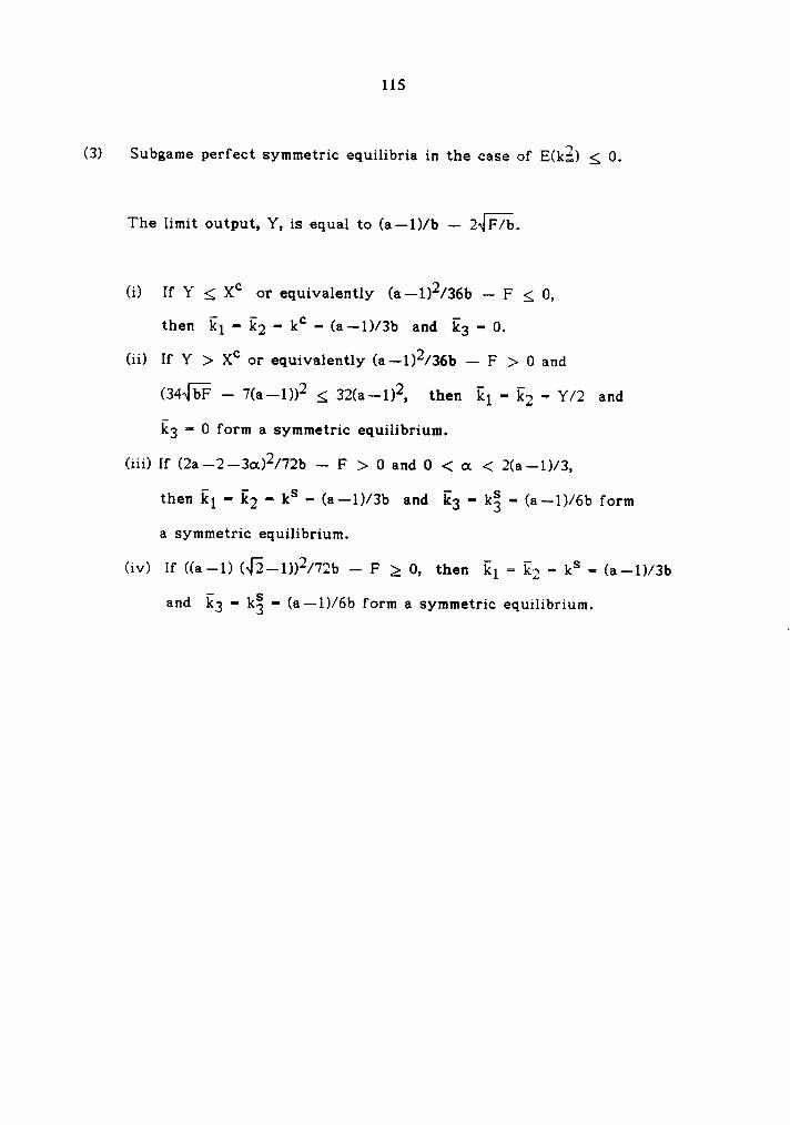
115

(3) Subgame perfect symmetric equilibria in the case of E(k?„) S 0.

The limit output, Y, is equal to (a—1)/b — 2«] F/b.

(i) If Y g Xc or equivalently (a-1)2/36b — F g 0,

then E1 - E2 - E° - ca-1)/ab ana E3 - 0.(ii) If Y > XC or equivalently (a—1)2/36b — F > 0 and

(34«]bF — 7(a—1))2 g 32(a—1)2, then kl = k2 - Y/2 and

k3 - 0 form a symmetric equilibrium.

(iii) If (2a—2—3o¤)2/72b — F > 0 and 0 < oc < 2(a—l)/3,

then kl - kg -ks — (a—1)/3b and E3 - kg — (a—1)/6b form

a symmetric equilibrium.

(iv) If ((a-1)(~E—1))2/72b — F 2 0, then kl = E2 = ks == (a—l)/3b

and k3 - kg - (a—1)/6b form a symmetric equilibrium.

capacity, entry deterrence, and … · other hand, acts as a stackelberg leader in output. if entry...

Documents