canine distemper virus impact on lion cheetah interactions ... · canine distemper virus impact on...
TRANSCRIPT

CANINE DISTEMPER VIRUS IMPACT ON
LION-CHEETAH INTERACTIONS IN THE
SERENGETI NATIONAL PARK
By Aliénor Chauvenet
Supervised by: Dr. Nathalie Pettorelli
Dr. Sarah Durant
Prof. Tim Coulson
A thesis submitted in partial fulfilment of the requirements
for the degree of Master of Science and the Diploma
of Imperial College London

2
ABSTRACT
The impact of human-induced threats on biodiversity is a constant concern for the
conservation community. Conservation projects are designed to decrease biodiversity loss
by removing threats towards species or ecosystems e.g. the creation of protected areas to
remove hunting pressure on a species. Sometimes, the creation of a protected area isn’t
enough and there is a need for additional human intervention e.g. removal of diseases or
invasive species. The Serengeti National Park (SNP), which was created as a human
intervention against game species depletion, is home to populations of two very
charismatic cats: the African lion Panthera leo and the cheetah Acinonyx jubatus. In the
plains of the SNP, they both persist in small populations. Unfortunately, the status of
National Park is not enough to guarantee the survival of either population residing in the
plains. The lion is vulnerable to a disease called canine distemper virus (CDV) due to the
huge population of domestic dogs (reservoir for the CDV) surrounding the park. The
cheetah, on the other hand, is under the pressure applied by lions as they kill cheetah cubs.
There may be the possibility of eradicating the CDV from the Serengeti by vaccinating
domestic dogs. However, the consequences of eradication on both cat populations need to
be assessed first.
I built two population models: an individual-based model for the cheetah and a
matrix population model for the lion. I then investigated the consequences of different
CDV outbreak rates on lion abundance and on cheetah population dynamics. I found that
there seems to be a direct link between lion abundance and cheetah abundance. With the
current outbreak rate (no interventions), the population of cheetahs in the Serengeti plains
is decreasing and if the CDV is eradicated, they may go extinct faster. Cheetahs may even
need an increase in CDV outbreak rates in order to be able to renew themselves. I found
that with the current CDV outbreak rate or after CDV eradication, there would only be half
the cheetah population left in 60 years.
This project shows possible shortcomings of species-based human-interventions.
By doing projects with the lion as sole focus (e.g. removing the CDV) conservationists
may further endanger the cheetah. On the other hand, being focused on the cheetah might
lead to promoting an increase in CDV occurrences which would in turn increase the chance
to lose lions as small populations are more vulnerable to stochastic events. Further work
should investigate how to optimally manage both species.
Word count: 12,300

3
LIST OF ACRONYMS
CITES Convention on International Trade of Endangered Species
CDV Canine Distemper Virus
IBM(s) Individual-based model(s)
IUCN International Union for Conservation of Nature
PA(s) Protected Area(s)
SNP Serengeti National Park

4
CONTENTS
I/ INTRODUCTION ............................................................................................ 7
1. Problem statement ....................................................................................... 7
2. Project significance ..................................................................................... 10
3. Aim and objectives ....................................................................................... 10
II/ BACKGROUND .............................................................................................. 11
1. Study site and species .................................................................................. 11
2. Population Dynamics: a general overview ................................................. 12
3. Cheetah population dynamics: what has been done .................................. 17
4. Lion impact on cheetah population dynamics: this project ......................... 17
III/ METHODS ...................................................................................................... 19
1. Model description ....................................................................................... 19
1.1 Lion matrix population model ............................................................. 19
1.2 Cheetah individual-based model ......................................................... 23
1.3 Coupling cheetahs with lions .............................................................. 25
2. Simulations..................................................................................................27
2.1 Testing model predictive power .......................................................... 27
2.2 Effect of different CDV outbreak rates on the cheetah population ..... 28
IV/ RESULTS ....................................................................................................... 29
1. Model fitting ................................................................................................ 29
1.1 Lion matrix population model (simulation a) ...................................... 29
1.2 Cheetah individual-based model (simulation b) .................................. 29
1.3 Coupling cheetahs with lions (simulations c and d) ............................ 30
2. Effect of different CDV outbreak rates on the cheetah population ............. 31
V/ DISCUSSION .................................................................................................. 38
ACKNOWLEDGMENTS ................................................................................... 43
REFERENCES ..................................................................................................... 44

5
FIGURES
Figure 1. Average cheetah population growth rate over 100 simulations when the cheetah
IBM is coupled with the lion matrix population model. Results depend on the simulation
timeframe (60, 50, 40 and 30 years) and the number of outbreaks per 60 years. ............... 34
Figure 2. Number of simulations where the populations have a negative growth rate (over
100 simulations). Results depend on the timeframe of the simulations (60, 50, 40 and 30
years) and the number of CDV outbreaks per 60 years ....................................................... 35
Figure 3. Number of simulations where the populations have a positive growth rate (over
100 simulations). Results depend on the timeframe of the simulations (60, 50, 40 and 30
years) and the number of CDV outbreaks per 60 years ....................................................... 35
TABLES
Table 1a. Population projection matrix for the Serengeti lions for years when there is no
CDV outbreaks. The reproduction rate Fx=0.8 unless the population has reached its
carrying capacity; in that case Fx=0..................................................................................... 21
Table 1b. Population projection matrix for the Serengeti lions for years where there is a
CDV outbreak. The reproduction rate Fx=0.8 unless the population has reached its carrying
capacity; in that case Fx=0 ................................................................................................... 22
Table 2. Initial cheetah population composition ................................................................. 23
Table 3. Monthly survival rates of the cheetahs in the Serengeti plains ............................ 24
Table 4. Published female lions abundance in the Serengeti National park (inferred from
Packer et al. 2005) ............................................................................................................... 25
Table 5. Expected ranking of r-squared values depending on which models are tested
against observed cheetah abundance. .................................................................................. 27

6
Table 6. Simulation parameters for when the cheetah IBM is coupled with the lion matrix
population model. Different outbreak rates are obtained by varying the CDV density-
dependent trigger, the CDV random number trigger or both .............................................. 28
Table 7. Results of the lion model simulations (1000 iterations). The table shows the lion
population growth rate for observed data (extracted from Packer et al. 2005) and predicted
with the lion model (using the ‘current’ parameters). The simulation timeframe is 29 years
allowing for the calculation of the r-squared between predicted and observed data ........... 29
Table 8. Simulation results of the cheetah IBM without the varying influence of lions; r-
squared is between model-predicted abundance and 16 years of observed adult males and
females abundance (Sarah Durant pers. comm. Dataset 1991-2006) .................................. 30
Table 9. Simulation results of cheetah IBM coupled with lion published abundance (c).
The lion data used are those observed from Packer et al. 2005; it provides lion numbers
from 1975 to 2003. Hence, the predicted cheetah abundance is compared with observed
date from 1991 to 2003 ........................................................................................................ 30
Table 10. Simulation results with ‘current’ parameters of lion model (d); correlation
between observed data (Table 4) and 16 years of predicted adult males and females
abundance (1991-2006) ....................................................................................................... 31
Table 11. Results of simulations (each of 100 iterations) of the cheetah IBM coupled with
the lion matrix population model. ‘+’ represents the number of cheetah populations for
which the average (Av.) λ>or =1 and, ‘-’ is the number of cheetah populations for which
the average λ<1, ‘/’ is the number of cheetah populations that went extinct ...................... 32
Table 12. Average number of cheetahs surviving in the Serengeti plains after 60 years
depending on how the number of CDV outbreaks during the timeframe ........................... 35
7
I/ INTRODUCTION
1. Problem statement
The world’s biodiversity is under threat and while the number of species on Earth and the
rate at which they are disappearing remain uncertain, there is evidence that the current rate
of species loss is much greater than historic ones (Millennium Ecosystem Assessment
2005). The principal causes for biodiversity loss are: habitat loss and degradation
(including land conversion, deforestation, and pollution), habitat fragmentation, climate
change, invasive species, overexploitation and diseases (Millennium Ecosystem
Assessment 2005). The common element of all those threats is that they are all more or
less human related.
The impact of human-induced threats on biodiversity is under constant study and,
conservationists have spent decades trying to halt or slow the rate of biodiversity loss. In
order to do that, many conservation projects have been designed to remove threats towards
species or ecosystems by using human interventions e.g. stop illegal logging (Hamilton et
al. 2000), remove invasive rats on islands (Towns and Broome 2003). One of the first lines
of defence against extinction is the creation of protected areas (PAs; Rodrigues et al.
2004). Protected Areas can take many forms e.g. they can be strict such as a National Park
or they can be designed to accommodate regulated hunting like a game reserve. The
motivations behind the creation of PAs are also varied e.g. protecting one patch of habitat,
one species or an ecosystem function. The design of PAs always depends on the target and
objectives the protected zone aims to achieve. Sometimes, the creation of a protected area
isn’t enough and there is a need for additional human intervention such as, for example,
removal of invasive species (Foxcroft et al. 2007).
One prominent example of human intervention is the Serengeti National Park
(SNP), Tanzania. First created as a hunting-free game reserve in 1929 in order to stop the
depletion of the Serengeti lion population, Panthera leo (Sinclair 1995), the SNP has now
full protection status and is a safe haven for many species. The SNP is notably home to
populations of two very charismatic cats: the African lion Panthera leo and the cheetah
Acinonyx jubatus.
Lions, which are the top predator of the SNP ecosystem, seem to be doing well in
the park. Observations reported in Packer et al. (2005) show that beyond yearly variation in
population size, the Serengeti lion population show an increasing trend. One of the threats
to their survival in the park is a disease called Canine Distemper Virus (CDV). In 1994, an
outbreak of CDV killed a third of the Serengeti lions (Roelke-Parker et al. 1996,

8
Woodroffe 1999). CDV exposure is however not always lethal, as studies of the Serengeti
lion CDV seroprevalence showed that lions had been previously exposed to the virus
without major death (Packer et al 1999). On the overall, the CDV affects four species in
the Serengeti region: lions, spotted hyenas Crocuta crocuta, bat-eared foxes Otocyon
megalotis and domestic dogs Canis lupus familiaris (Roelke-Parker et al. 1996, Carpenter
et al. 1998) but has no incidence on the cheetah. Murray et al. (1999) found that the CDV
is transmitted to lions and hyenas from the domestic dog which acts as a ‘reservoir’
species. There are currently around 30,000 domestic dogs around the Serengeti (Roelke-
Parker et al. 1996), and thus, the potential for a CDV outbreak remains constant. One way
of reducing the impact of CDV on the Serengeti lion population is to vaccinate the dogs
surrounding the SNP against the virus. Such procedure would go toward the conservation
of the lion, a highly charismatic species which is classified as vulnerable on the IUCN red
list (IUCN 2009).
Cheetahs, which are on the Appendix I of the Convention on International Trade of
Endangered Species of Wild Fauna and Flora (CITES), are also listed as vulnerable on the
IUCN red list and have suffered from a range-wide decline in the past decades (IUCN
2009). Like other carnivores, they face several human-induced threats at the species level,
notably habitat loss and persecution by humans (IUCN 2009). However, in the plains of
the SNP, their population size is known to be limited by other factors. In the early 1980s,
the SNP cheetahs were thought to be at genetic bottleneck: at that time, both little genetic
variation and inbreeding were thought to be responsible for their low population number
and survival rates (O’Brien et al. 1985). However, in depth ecological studies proved that
the low density of cheetahs was, in fact, due to cub being killed by lions and spotted
hyenas (Caro 1987, Laurenson 1994; Kelly & Durant 2000). Laurenson (1995) found that
lion predation is one of the biggest threats to cub survival and that cheetah biomass is
inversely correlated with lion biomass across protected areas in the African sub-Sahara,
suggesting that lions play an important role on cheetahs’ number regulation. Beyond
competing for food with the cheetahs, lions can also easily kill an adult (Laurenson 1995).
However, they tend to attack the newborn cubs which are still in the lair, very often killing
the entire litter (Laurenson 1995, Pettorelli & Durant 2007a). As lions were shown to be
responsible for the very low cheetah cub survival rate in the SNP, and as cheetah biomass
was previously reported to be inversely correlated with lion biomass across the African
sub-Sahara, I can safely hypothesize that variation in lion density should affect cheetah
population dynamics. There are several examples, in nature, where the decrease or removal

9
of a top-predator has led to an increase of a mesopredator. The ‘mesopredator release
effect’ theory (Courchamp et al. 1999, Ritchie et al. 2009) states that as a community top-
predator decreases or is removed, mesopredators are free to expand their niches as more
food becomes available and/or predation pressure on its population decreases (e.g., the
extinction of jaguars Panthera onca on Barro Colorado Island has led the puma Puma
concolor and ocelot Leopardus pardalis shifting their diets to bigger prey, Moreno et al.
2006). However, although lions and cheetahs can compete for food, the reason for which
cheetahs would benefit from a reduction in lions is not the resulting increase in food
availability (Durant et al. in press). A decrease in lions’ numbers would result in the
increase in cheetahs’ numbers because the direct predation pressure on cheetahs’ cubs
would lessen.
In the SNP, there are therefore two charismatic species that are equally loved by the
international community and classified as vulnerable on the IUCN red list (IUCN 2009).
The problem resides in the fact that (1) although they are increasing on the overall, the
SNP lions’ number remains below 200 (Packer et al. 2005) which make them particularly
vulnerable to environmental stochasticity, therefore, to a new epidemic of CDV (Kendall
1998) and (2) the cheetahs’ number are also very low (less than 100 adults; Sarah Durant
pers. comm.), they have previously been found to be decreasing and their number is known
to be limited by the lions (Kelly and Durant 2000). As population sizes within a guild are
limited by competition, predation or a mix of both (Holt and Pickering 1985) and as a
factor affecting one species’ population size can end up affecting the entire guild (Levin
1970), a CDV outbreak (or the disappearance of such a virus) could greatly impact the lion
numbers and in return the cheetah numbers. It is expected that the higher the number of
CDV outbreaks the lower the number of lions and therefore the higher the number of
cheetahs. On the other hand, the total removal of the CDV could lead the lion population to
increase and the cheetah population to further decrease.
Before considering human-intervention such as the vaccination of the domestic dogs
against CDV, there is a need to assess the consequences that eradication would have on the
populations of cheetahs and lions in the SNP. By being species driven, human intervention
in the SNP could lead to unintentional conservation triage (Possingham 2002), that is,
prioritizing one species over the other leading to the disappearance of the non-target.

10
2. Project significance
The world biodiversity is declining (Millennium Ecosystem Assessment 2005). As a
response to threatened biodiversity, protected areas have been created to protect species
under threats (Lee and Jetz 2008). The SNP is protecting the lions by removing human
pressure on this much-loved species. However, due to the laws of predation and
competition, while lions are fine, cheetah numbers are not increasing, especially in the
Serengeti plains, leading to the belief the Serengeti cheetah survival depends on the lion
population remaining at a certain level. A natural form of control over the Serengeti lion’s
population number is the Canine Distemper Virus. While the CDV is always silently
present in the lion population, it can eventually lead to an epidemic; it did in 1994,
reducing lion numbers by a third (Roelke-Parker et al. 1996). However, there is the
possibility of eradicating the CDV from the Serengeti, removing the control over the lion
population. This could have catastrophic consequences for cheetahs in the Serengeti plains.
There is therefore an obvious conflict. While conservationists want nothing more than
protect the world species, good-intentioned human intervention could cause the accidental
disappearance of a whole population. As a result, understanding the effect of variation in
the lion population on the cheetah population can lead to being able to predict the response
of the cheetah population if the lion population increases (e.g. due to an increase in preys
or the disappearance of the CDV) or decreases (e.g. after a CDV outbreak).
3. Aims and Objective
This project aims at understanding the impact of variation in the SNP lion abundance on
the SNP cheetah population numbers by modelling the cheetah population dynamics when
coupled with a lion population undergoing different CDV epidemic rates.
In order to reach that aim, I will:
1. Build an age-structured matrix population model for the lion population
where I can control the number of CDV outbreaks hitting the population
over time.
2. Build an individual-based model for the cheetah population where
individuals have different survival and reproductive abilities.
3. Couple both models and investigate the effect of variable occurrence of
CDV outbreaks on lion and cheetah population dynamics.
11
II/ BACKGROUND
1. Study site and species
The Serengeti is a 30,000 km² ecosystem that extends over the border between of Tanzania
and Kenya; it is defined by the migration range of the wildebeests, Connochaetes taurinus
(Sinclair 1995). The main feature of this exceptional ecosystem is the amount of
biodiversity that resides within it. In addition to high diversity of carnivores (the largest
concentration in the world) and birds, there are 28 species of ungulates living in the
Serengeti and herds are bigger than anywhere else in the world (Sinclair 1995). There are
several conservation administrations within this ecosystem: Ngorongoro Conservation
Area, Serengeti National Park, Maswa game reserve, Masai Mara National Reserve. The
SNP was established in the early 1950s, following the region being declared a hunting-free
game reserve (Caro 1994, Sinclair 1995). Although, at the beginning, it encompassed the
Ngorongoro craters and its northern limit stopped below the Kenyan border, since 1965 the
national park has ceased to include the former and has been extended to include the current
Kenyan outstretch.
This project focuses on two species: the cheetah and the lion. They both occur
throughout the SNP but I will focus on the populations that live in the Serengeti plains.
These grassy plains are located in the south-eastern part of the SNP and cover an area close
to 5,000 km² (Caro et al. 1987, Caro 1994).
In the SNP, cheetahs are found in both the plains and the woodlands, however,
there is extensive observational data on the plains population. Their lifecycle can be
divided into four stages: pre-weaning small cubs (1 to 3 months old), large cubs (4 to 12
months old), adolescents (13 to 24 months old) and adults (>2 year of age). Cheetah
females are solitary and occupy overlapping home ranges, while males can be solitary,
territorial, and/or form coalitions (Caro 1994). Male territory size averages 48 km², whilst
solitary males and females can range over 800 km² (Caro 1994). From two years old,
female cheetahs are reproductively active. The largest litter ever recorded is seven cubs
(observed once; Sarah Durant, pers. comm.) but usually the maximum of cubs produced
per litter is six (Kelly and Durant 2000) Females can become pregnant before the current
litter leaves the mothers’ side, however, the family will separate before the new cubs are
born. If the female loses a litter, she can enter oestrous rapidly (Caro 1994) and produce a
new litter in about 4 months (Crooks et al. 1998). Once the adolescents have left their
mothers, they can stay in a sibling group for up to 6 months, after which females leave to
be solitary and have their first litter (Caro 1994). During the first year, and particularly the

12
first two to three months, cubs are extremely vulnerable to lions’ attack (Laurenson 1994).
The lions will usually kill the whole litter (Laurenson 1995). The pressure that lions inflict
on cheetahs is such that in 1994, Laurenson recorded that of all the cubs death that could
be attributed a reason, a bit less than 70% was due to lion killing them. The relationship
between cheetahs and lions is one of occasional competitors but mostly predator-victims:
as lions do not feed on the cubs they kill, the word prey doesn’t describe the situation
accurately, and hence cheetahs should more accurately be referred to as lions’ victims.
Lions are territorial, highly social species. They live in prides that are composed of
2 to 9 adult females and 2 to 6 adult males (Hanby et al. 1995). In addition, the prides
contain the females’ dependent young. In the SNP, lions reside in the plains and the
woodlands alongside the cheetahs. Lions feed principally on migratory species such as
wildebeest and zebra, Equus burchelli, and therefore endure high fluctuations in food
availability (Scheel and Packer 1995). Females can start reproducing once they reach four
years of age and can live up to 18 years old (Clutton-Brock 1988).
Both species have been studied for decades (Scheel and Packer 1995, Durant el al.
2007). There is, therefore, extensive information available on them in the published
literature. Records of cheetahs’ abundance (adults and adolescents of both sexes) for the
period of 1991 to 2006 have been obtained from Sarah Durant (pers. comm.) while lion
abundance was recovered from Packer et al. (2005).
2. Population dynamics: a general overview
To study population dynamics is to investigate how a population composition evolves over
time (Williams et al. 2001). At its simplest, the number N of individuals in a population at
time t+1 depends on the number of individuals at the time-step before (time t) and the birth
and death that have occurred in the transition from t to t+1. If the population is not isolated
from others, individuals can join or leave it, also influencing the population composition.
Therefore:
(1)
Slightly more complicated mathematical models have been created to better describe the
dynamics of a population. Equation (2) below, is best suited for populations that have
breeding seasons where there is a sudden population increase at a regular time-step. In
such approach, the population at the next time-step t+1 is defined as a function of the
population at the current time-step Nt and the finite population rate of growth λ:

13
(2)
The parameter λ determines the trajectory of the population. If λ=1, the population is
replacing itself whereas if it is λ<1, the population is decreasing over time. However, if
λ>1, the population is increasing. On the other hand, equation (3) is more suited for
populations that breed all year long with no sudden increase. The population composition
at t+1 is once again determined by Nt but also by the intrinsic growth rate r. Here,
(3)
The relationship between the finite growth rate λ and the intrinsic growth rate r is:
(4)
Those simple equations, however, describe populations with unrestricted growth, which
would equal to an infinite supply of resources (food, habitat, etc...). Moreover, equations
(2) and (3) assume that the birth and death rates are constant and that all individuals can be
described with the same parameters’ values because they’re considered as being equal (no
individual heterogeneity). By considering all individuals to be equal (over time and space),
equations (2) and (3) assume that the population is not under the influence of demographic
or environmental stochasticity. Demographic stochasticity represents the variations
between individuals within the population that result from random events in survival and
reproduction (e.g. some individuals will survive longer or have more offsprings; Shaffer
1987, Kendall 1998). Environmental stochasticity represents variations that result from the
weather, food supply or populations of competitors and predators (Shaffer 1987; Kendall
1988). Demographic and environmental stochasticities both occur to different extent in
every species and ignoring them can lead to a poor representation of a system.
To attempt at modelling population dynamics closer to reality, there are equations
that take into account the fact that population growth isn’t infinite. The logistic growth rate
equation incorporates a new parameter: K or carrying capacity. The carrying capacity
represents the number to which the population can grow before density-dependent self-
regulation forces the population to stabilise (Fowler 1981). K can be determined by many
factors (e.g., food availability, predator number). As a result the value of K can vary
temporally for the same population. To simplify the use of the carrying capacity, its value
is generally assumed to be constant while the self-regulation response to reaching K is
assumed to be immediate. In such situation, the population growth model can be described
as:
(5)

14
Equation (5) can also be adjusted to describe a population that is harvested by removing a
portion of the population at each time-step. It has, in addition, been adapted to model two
common interactions between populations: prey-predator and resource competition. Those
two models are called: ‘Lokta-Volterra transition equation’ and ‘Lokta-Volterra’
completion model’ respectively (Williams et al. 2001, Rockwood 2006).
So far, I have described models where no individual variability is considered. It is
however possible to incorporate some of this variability by aggregating individuals
according to their sex or age, creating models with increased predictive power. The idea is
to divide the population into smaller units of individuals sharing a trait or character.
Instead of approximating one intrinsic growth rate for the entire population, variation in r
is allowed by e.g. attributing different values of r to every age category. Let’s consider for
example a population whose individuals can be aggregated in x=3 age categories. Each age
category has an individual intrinsic growth rate rx and a number of individuals Nx at time t.
At time t+1, the total population is therefore composed of:
(6)
Equation (6) describes the composition of the entire population by considering each
age category to be isolated, hence individuals can’t move from one to another in the course
of their lives. However, individuals do move from one age category to another as they
grow older. To model a population where there is a transition between age categories, the
population’s life cycle needs to be identified (Caswell 2001). The two key parameters of
life cycles are reproduction and survival; these are also called vital rates and can be defined
as age- and/or sex-specific. Those vital rates will have different influences on the dynamic
of a population. For example, the factors that have the strongest influence on cheetah’s
population dynamics are adult and cub survival (Kelly and Durant 2000). In order to
determine which parameters are most important for a population, a perturbation analysis
can be performed. Its results are expressed as sensitivities and elasticities (Caswell 2001,
Caswell 2009) e.g. the sensitivity of λ to adult survival. Sensitivity informs on how a
parameter y will change if a parameter x changes. Elasticity is the proportional response of
a parameter to a proportional change in another (Caswell 2001).
Life cycles are used in matrix population modelling (Caswell 2001). A matrix is
built following a fundamental principal: a population will grow over time but not without
limits. As a result a matrix population model can account for a small amount of individual
heterogeneity and also be density-dependent. The population is divided into classes of

15
similar individuals. To design the matrix, the population is divided into discrete classes to
which we will apply class-specific parameters. At time t the population will be composed
of a certain number n of individuals in each class xnt .The aim is to project the number of
individuals at time t+1. At time t+1, the individuals that were in classes xt at time t will
have moved to class xt+1 if they survived and new individuals are born and enter the matrix.
Matrix based models have often been used in the literature to solve various
problems. For example, O’Connor et al. (1993) used a size-structured matrix population
model to investigate the population growth rate of six perennial African grasses under
different fire regimes. In 2000, Bro et al. used matrix modelling to look at the state of
French populations of the grey partridge Perdix perdix. This type of population modelling
was also used to study the reintroduction success of the black-footed ferret Mustela
nigripes in Northern America, establishing that the first year survival rate is the most
important rate for the ferret persistence (Grenier et al. 2007). Matrix population models
were also used to look at the fire management and density dependence of the restoration
success of longleaf pine forest Pinus palustus in the US (Cropper and Loudermilk 2006).
There is another option for modelling population dynamics; one that allows for true
individual variation: individual-based models (IBMs). Like matrix models, IBMs have
been used in ecology for years (Grimm et al. 2005b, Nehrbass and Winkler 2007). While
the former utilizes a top-down approach, that is, model the population to infer things about
the individual, the latter uses a bottom-up approach. Indeed, in individual-based modelling,
the smaller parts of a system are assembled first, the individuals, in order to infer things
about the entire system: the population (Grimm 1999, Reuter et al. 2005). Ecological
systems are complex entities and using simpler models sometimes isn’t enough to capture
the relationships that need to be represented. Some of the problems with more classic
models (as opposed to IBMs) are that they don’t account for the high number of
components of the system and their variability, the spatial and temporal scale within which
species operate, context-sensitive actions or feedback loops such as, for example, how
density-dependence might influence future generation size (deRoos et al. 2003, Reuter et
al. 2005). Non-individual-based models have a lot of generalization potential but it comes
at the cost of closeness to reality. IBMs on the other hands are more flexible but require
more data to implement. The definition of an individual-based model is a simulation model
that treats individuals as unique and discrete entities that have at least one property that
changes during their life cycle beside age e.g. weight, predation susceptibility,
reproductive output (Grimm 1999, Grimm and Railsback 2005). Therefore, by allowing for

16
individual variability, IBM can be closer to reality but also more complex. As a result it is
essential to find the right balance between the amount of details and the general application
of the model. Indeed, the more details in the model the more complex and case-specific it
is going to be; hence less likely to be used to derive general ecological rules. However, by
reducing the amount of details too much, there is the risk of losing the benefits of treating
each individual as unique, like they actually are: better representation of reality (Grimm
and Railsback 2005). There are no standards in constructing an IBM like there is for matrix
models and IBMs require an amount of data that is not available for all species. That type
of modelling cannot, therefore, always be used to model an ecological system. As there are
no standard guidelines to build an IBM, the construction of one must rely on ‘patterns’ that
have emerged from the observations of the system the model is trying to represent. Patterns
are rules that will determine how each individual will evolve spatially or temporally
(Grimm et al. 2005, Grimm 1999). There are several limitations to using IBMs; as pointed
out before, there is a trade-off between the complexity of the model and how it will be
possible to interpret it. IBMs are also not easily described by mathematical formulas and
common language, which makes it hard to communicate the results or allow for
verification and replication by others. The data requirement is extensive and rarely
available. Moreover, if adequate data is available, IBMs are highly specific as opposed to
generalized modelling. Finally, the lack of standards results in models built from scratch
using ad-hoc assumptions (Grimm and Railsback 2005). Regardless, IBMs have been used
exponentially since 1988 when Huston et al. published a review criticizing modelling
assuming that individuals making up a population are identical and that each individual has
the same interaction with all its conspecifics. Since then, IBMs have been used in varied
situations e.g. model fish reproductive output (Scott et al. 2006), investigate the impact of
biological control on an introduced plant (LeMaitre et al. 2008), explore tree-tree intra-
specific competition (Caplat et al. 2008) and model predator-prey interactions in a small
rodent community (Reuter 2005). Moreover, in 2007, Nehrbass and Winkler used
individual-based modelling to assess the spread of the invasive German hogweed
Heracleum mantegazzianum. They compared their results to a previous simpler matrix
model and found that modelling individuals as autonomous entities made the results closer
to reality.

17
3. Cheetah population dynamics: what has been done
There have been a few attempts at modelling the population dynamics of the cheetah. In
1995, Laurenson attempted to look at cheetah population dynamics in the SNP using a
simple mathematical model of birth, death and recruitment, and found that high juvenile
mortality severely limits cheetah abundance. Berry et al. (1997) found concurrent results
through a population viability analysis (PVA; using Vortex, Lacy et al. 2005), estimating
that the cheetah population of Namibia is limited by cub mortality but also adult human-
induced mortality. In 1998, Crooks et al. created an age-structured matrix population
model with data from the Serengeti cheetah and came to a different conclusion, saying that
actually, adult mortality has the most influence on cheetahs’ population numbers. In 2000,
a more complex PVA was conducted by Kelly and Durant (2000). They used long-term
demographic data (20 years observation data) on the SNP cheetahs to estimate the
population growth rate (λ). They also analysed cheetahs’ extinction risk using the
stochastic model Popgen (Durant 1991) and investigated the effect of different lion
densities on juvenile survival. They came to the conclusion that (1) the Serengeti cheetah
population growth rate is most sensitive to adult and juvenile survival, (2) the population
growth rate λ was close to 1 (λ =0.997) during the 20 year study (1975-1994), revealing no
strong population trend, and (3) high lion abundance (the highest ever recorded during the
study: 120 adult females) would lead to cheetahs going extinct in the next fifty years.
All these attempts at understanding cheetah population dynamics have highlighted
the fact that the juvenile and adult survivals have a major role in limiting cheetah numbers.
However, according to Kelly and Durant (2000), cub survival is much more likely to vary
than adult survival making cub survival the most determinant factor in cheetah population
dynamic. These models, nonetheless, do not take into account the high individual
variability in survival and reproduction previously reported in cheetahs (Caro 1994;
Pettorelli & Durant 2007a,b; Durant et al. in press). It is expected that better integrating
individual variability in cheetah population dynamics models would increase the predictive
power of the models. One way to model individual variability is to use individual-based
modelling. With a small population like the cheetahs in the Serengeti plains that has been
studies for several decades, IBM seems to be a highly feasible and appropriate choice.
4. Lion impact on cheetah population dynamics: this project
For this project individual-based modelling will be used to model the dynamics of the
cheetah population of the Serengeti plains. I have a dataset containing 16 years of

18
population monitoring (number of adults and adolescents of both sexes each year; Sarah
Durant, pers. comm.). In addition, the cheetah is a very well studied species, providing me
with published demographic information usable in the model. From those published studies
(Crooks et al. 1998, Kelly and Durant 2000, Durant et al. in press) have arisen patterns that
can be used in this model, guaranteeing the right amount of complexity and limited
uncertainties. One of the main criticisms addressed at IBM is the lack of generality. This
model purpose is to be a predictive tool for the Serengeti cheetah population, which allow
us to be species-specific. IBM performance can be tested against the observed population
numbers from the 16 years dataset by calculating the population growth rate λ and r-
squared between observed and predicted adult male and female numbers.
As far as the Serengeti lions are concerned, matrix population modelling will be
used as a simpler way to model their population dynamics. The lion matrix population
model will be a female-based age-structured model and will take into account the impact of
canine distemper virus on lion abundance. By creating a model for the lion population
(instead of using lion numbers as covariates for example) I can control the number of CDV
outbreaks during a given period of time. The occurrence of an outbreak is controlled by
two factors: density-dependence (the lions must have reached a certain number) and
stochasticity (there is a random chance that even if the population reaches the right
abundance an outbreak will actually not occur). The lion matrix population model does not
account for the fact that lions are organised in prides. The highly structured nature of lion
population plays an important part in female survival and reproduction as both depend on
territoriality and synchronous breeding (Packer et al. 2001). I, however, have to rely on
published data to create the model and cannot make the lion model as realistic as it would
need to be. As a result, it is going to be less accurate.
Those two models will then be coupled to investigate the link between lion
abundance and cheetah abundance based on the fact that (1) lions influence the cheetah
cubs’ survival rate (0 to 1 year old) and (2) the CDV plays an important role in regulating
lion numbers.

19
III/ METHODS
1. Model description
1.1. Lion matrix population model
I used a female-only age-structured matrix population model (assumes a 1:1 ratio of
females to males) to represent the Serengeti lions’ population (x=18 age classes of one
year). According to Ogutu et al. (2002), the lion population composition is: 20% small
cubs (0 to 1 year old), 10% large cubs (1 to 2 years old), 15% sub-adults (2 to 4 years old)
and 55% adults (>4 years old). I used an initial population number of 35 females based on
the population number reported in Packer et al. (2005) and split the initial female
population according to the percentages above e.g. 10% in the 0-1 class, 20% in 1-2 class,
(15/2)% in 2-3 and 3-4 class, (55/14)% in the remaining classes.
I inferred the lion age-specific survival rates and CDV mortality rates in the
Serengeti from Kissui and Packer (2004; Table 1a and b). Lions can reproduce once they
enter the 3 to 4 age class (once they have survived beyond 3 years old; Clutton-Brock
1988) until they reach 13 years old. The reproductive rate is the same for every
reproducing class x: Fx= 0.8 females (Clutton-Brock 1988).
The model is density dependent. Based on values reported in Packer et al. (2005),
the initial carrying capacity was set as 60 females but it can vary throughout the simulation
as a way to replicate bad, average and good years (e.g., a good year can be a wet year when
there are a lot of prey as opposed to a dry year when prey density is lower). If the carrying
capacity is at 60, it can drop to 40 or increase to 80; there is an equal chance of either. As I
do not have quantitative data on changes in carrying capacity and there is no obvious
pattern emerging from the data presented in Packer et al. (2005), the most sensible way to
vary the carrying capacity from 60 is, therefore, to give it an equal chance of increasing or
decreasing. If the carrying capacity is at 80, it can only decrease to 60 and if it is 40, it can
only increase to 60. This ensures that the changes are not too dramatic. The change in
carrying capacity is triggered by the comparison between a random number (taken from a
uniform distribution) and a set trigger number. I use the number 0.8 as a trigger for a
carrying capacity change. The choice of trigger number is based on a rule of thumb rather
than empirical data. From Packer et al. (2005) it seems that the carrying capacity changes
less often than every year. Therefore, I chose a number that makes a change relatively rare.
If the random number is >0.8, the carrying capacity changes according to the pattern
described above. If the total number of females at time t is equal to or above the carrying
capacity at the current time-step, it is assumed that the shortage of resources will prevent

20
the population from increasing. The actual consequences of reaching K haven’t been
quantified for the lion (at least in available published data); however, there is a supported
theory that states that as a population reaches its carrying capacity one consequence is a
decrease in reproductive rate of adult females (Eberhardt 2002) and I modelled the impact
of reaching at carrying capacity by setting the next time-step fecundity to zero: Fx(t+1)=0
(Table 1b).
An outbreak of CDV becomes possible when the female number is equal or above
60 which simulates the population susceptibility to being infected, e.g. the higher the
density of lions the higher the chance to come in contact with an infected animal (Packer et
al. 1999). I used a density-dependent CDV trigger since in Packer et al. (2005), the 1994
epidemics which claimed a third of the Serengeti lions happened after a peak in population
number, supporting the hypothesis that CDV outbreaks have a density-dependence
component. If the population reaches 60, the model compares a random number (from a
uniform distribution) to a number trigger of 0.8 which simulates the need for a certain
number of infected individuals to get an epidemic; the higher the CDV trigger is the harder
it is to have an outbreak. If the random number is above 0.8, the population suffers from a
CDV outbreak and the survival rates used to project the population from t to t+1 are the
one from Table 1b. Based on published data, there has been 1 epidemic in 29 years (in
1994) and by using both CDV parameters of 60 females and number trigger of 0.8 I
managed to simulate 2 epidemics in a 60 years time frame which is close to reality.
The population can be projected over any timeframe but in order to compare the
model predictions with the values reported in Packer et al. (2005) from 1975 to 2003, I
used a 29 years timeframe. The simulations were run over 1000 iterations. For the lion
population model alone I calculated the population growth rate λ. In order to do that, at
each time step t, I determined the ratio: , N being the total number of individuals in the
population and take the average of all the values obtained. The λ from the observed values
reported in Packer et al. (2005) is 1.05, and I expected the λ of the model to show an
increasing population trend as well. I also calculated the mean r-squared between both
observed and predicted lion abundance.

21
Table 1a. Population projection matrix for the Serengeti lions for years when there is no CDV outbreaks. The reproduction rate Fx=0.8 unless the
population has reached its carrying capacity; in that case Fx=0.
x 0-1 1-2 2-3 3-4 4-5 5-6 6-7 7-8 8-9 9-10 10-11 11-12 12-13 13-14 14-15 15-16 16-17 17-18
0-1 0.0 0.0 0.0 F3-4 F4-5 F5-6 F6-7 F7-8 F8-9 F9-10 F10-11 F11-12 F12-13 F13-14 0.0 0.0 0.0 0.0
1-2 0.4 0.0 0.0 0.0 0.0 0.0 0.0 0.0 0.0 0.0 0.0 0.0 0.0 0.0 0.0 0.0 0.0 0.0
2-3 0.0 0.9 0.0 0.0 0.0 0.0 0.0 0.0 0.0 0.0 0.0 0.0 0.0 0.0 0.0 0.0 0.0 0.0
3-4 0.0 0.0 0.9 0.0 0.0 0.0 0.0 0.0 0.0 0.0 0.0 0.0 0.0 0.0 0.0 0.0 0.0 0.0
4-5 0.0 0.0 0.0 0.9 0.0 0.0 0.0 0.0 0.0 0.0 0.0 0.0 0.0 0.0 0.0 0.0 0.0 0.0
5-6 0.0 0.0 0.0 0.0 0.9 0.0 0.0 0.0 0.0 0.0 0.0 0.0 0.0 0.0 0.0 0.0 0.0 0.0
6-7 0.0 0.0 0.0 0.0 0.0 0.9 0.0 0.0 0.0 0.0 0.0 0.0 0.0 0.0 0.0 0.0 0.0 0.0
7-8 0.0 0.0 0.0 0.0 0.0 0.0 0.9 0.0 0.0 0.0 0.0 0.0 0.0 0.0 0.0 0.0 0.0 0.0
8-9 0.0 0.0 0.0 0.0 0.0 0.0 0.0 0.9 0.0 0.0 0.0 0.0 0.0 0.0 0.0 0.0 0.0 0.0
9-10 0.0 0.0 0.0 0.0 0.0 0.0 0.0 0.0 0.9 0.0 0.0 0.0 0.0 0.0 0.0 0.0 0.0 0.0
10-11 0.0 0.0 0.0 0.0 0.0 0.0 0.0 0.0 0.0 0.9 0.0 0.0 0.0 0.0 0.0 0.0 0.0 0.0
11-12 0.0 0.0 0.0 0.0 0.0 0.0 0.0 0.0 0.0 0.0 0.9 0.0 0.0 0.0 0.0 0.0 0.0 0.0
12-13 0.0 0.0 0.0 0.0 0.0 0.0 0.0 0.0 0.0 0.0 0.0 0.9 0.0 0.0 0.0 0.0 0.0 0.0
13-14 0.0 0.0 0.0 0.0 0.0 0.0 0.0 0.0 0.0 0.0 0.0 0.0 0.7 0.0 0.0 0.0 0.0 0.0
14-15 0.0 0.0 0.0 0.0 0.0 0.0 0.0 0.0 0.0 0.0 0.0 0.0 0.0 0.7 0.0 0.0 0.0 0.0
15-16 0.0 0.0 0.0 0.0 0.0 0.0 0.0 0.0 0.0 0.0 0.0 0.0 0.0 0.0 0.6 0.0 0.0 0.0
16-17 0.0 0.0 0.0 0.0 0.0 0.0 0.0 0.0 0.0 0.0 0.0 0.0 0.0 0.0 0.0 0.4 0.0 0.0
17-18 0.0 0.0 0.0 0.0 0.0 0.0 0.0 0.0 0.0 0.0 0.0 0.0 0.0 0.0 0.0 0.0 0.1 0.0
18+ 0.0 0.0 0.0 0.0 0.0 0.0 0.0 0.0 0.0 0.0 0.0 0.0 0.0 0.0 0.0 0.0 0.0 0.0

22
Table 1b. Population projection matrix for the Serengeti lions for years where there is a CDV outbreak. The reproduction rate Fx=0.8 unless the
population has reached its carrying capacity; in that case Fx=0.
x 0-1 1-2 2-3 3-4 4-5 5-6 6-7 7-8 8-9 9-10 10-11 11-12 12-13 13-14 14-15 15-16 16-17 17-18
0-1 0.0 0.0 0.0 F3-4 F4-5 F5-6 F6-7 F7-8 F8-9 F9-10 F10-11 F11-12 F12-13 F13-14 0.0 0.0 0.0 0.0
1-2 0.3 0.0 0.0 0.0 0.0 0.0 0.0 0.0 0.0 0.0 0.0 0.0 0.0 0.0 0.0 0.0 0.0 0.0
2-3 0.0 0.6 0.0 0.0 0.0 0.0 0.0 0.0 0.0 0.0 0.0 0.0 0.0 0.0 0.0 0.0 0.0 0.0
3-4 0.0 0.0 0.7 0.0 0.0 0.0 0.0 0.0 0.0 0.0 0.0 0.0 0.0 0.0 0.0 0.0 0.0 0.0
4-5 0.0 0.0 0.0 0.8 0.0 0.0 0.0 0.0 0.0 0.0 0.0 0.0 0.0 0.0 0.0 0.0 0.0 0.0
5-6 0.0 0.0 0.0 0.0 0.9 0.0 0.0 0.0 0.0 0.0 0.0 0.0 0.0 0.0 0.0 0.0 0.0 0.0
6-7 0.0 0.0 0.0 0.0 0.0 0.7 0.0 0.0 0.0 0.0 0.0 0.0 0.0 0.0 0.0 0.0 0.0 0.0
7-8 0.0 0.0 0.0 0.0 0.0 0.0 0.7 0.0 0.0 0.0 0.0 0.0 0.0 0.0 0.0 0.0 0.0 0.0
8-9 0.0 0.0 0.0 0.0 0.0 0.0 0.0 0.7 0.0 0.0 0.0 0.0 0.0 0.0 0.0 0.0 0.0 0.0
9-10 0.0 0.0 0.0 0.0 0.0 0.0 0.0 0.0 0.7 0.0 0.0 0.0 0.0 0.0 0.0 0.0 0.0 0.0
10-11 0.0 0.0 0.0 0.0 0.0 0.0 0.0 0.0 0.0 0.7 0.0 0.0 0.0 0.0 0.0 0.0 0.0 0.0
11-12 0.0 0.0 0.0 0.0 0.0 0.0 0.0 0.0 0.0 0.0 0.5 0.0 0.0 0.0 0.0 0.0 0.0 0.0
12-13 0.0 0.0 0.0 0.0 0.0 0.0 0.0 0.0 0.0 0.0 0.0 0.5 0.0 0.0 0.0 0.0 0.0 0.0
13-14 0.0 0.0 0.0 0.0 0.0 0.0 0.0 0.0 0.0 0.0 0.0 0.0 0.5 0.0 0.0 0.0 0.0 0.0
14-15 0.0 0.0 0.0 0.0 0.0 0.0 0.0 0.0 0.0 0.0 0.0 0.0 0.0 0.5 0.0 0.0 0.0 0.0
15-16 0.0 0.0 0.0 0.0 0.0 0.0 0.0 0.0 0.0 0.0 0.0 0.0 0.0 0.0 0.3 0.0 0.0 0.0
16-17 0.0 0.0 0.0 0.0 0.0 0.0 0.0 0.0 0.0 0.0 0.0 0.0 0.0 0.0 0.0 0.0 0.0 0.0
17-18 0.0 0.0 0.0 0.0 0.0 0.0 0.0 0.0 0.0 0.0 0.0 0.0 0.0 0.0 0.0 0.0 0.0 0.0
18+ 0.0 0.0 0.0 0.0 0.0 0.0 0.0 0.0 0.0 0.0 0.0 0.0 0.0 0.0 0.0 0.0 0.0 0.0

23
1.2. Cheetah individual-based model
Conversely to the lion population model, the cheetah individual-based model accounts for
both males and females. The population is structured in four categories: 0-3 months old (small
cubs), 4 to 12 months old (large cubs), 13 to 24 months old (adolescents) and >25 months old
(adults). The model follows each individual throughout their life cycle by monthly
increments. The initial population number and composition correspond to year 1991 of the
1991-2006 dataset available on the Serengeti cheetahs (Sarah Durant pers. comm.; see Table
2). The dataset, however, does not contain the number of 0-1 year old cubs as it very hard to
estimate cub abundance for two reasons: during the first 2 to 3 months of life the small cubs
stay hidden in the lair and births can be unrecorded if the mother is not spotted at the right
time (Kelly and Durant 2000). After performing a 12-months simulation (100 iterations), I
found that the average annual number of cubs produced is around 60. The sex ratio being 1:1
(Caro 1994), I started the population with 30 cubs of each sex. Nonetheless, after trying with
several initial cub number (from 10 to 60 per sex), it appeared that this number had very little
influence on the model performance.
Table 2. Initial cheetah population composition
Age group (in months) Males Females
0-12 30 30
13-24 4 5
25+ 17 37
The monthly survival rates of each age-class were extracted from published literature
(see Table 3). However, the survival rates of the small cubs (0-3 months old) published in
Crooks et al (1998) and Kelly and Durant (2000) are both very small (0.03 and 0.10 yearly
survival rate respectively). Those rates come from observed data on a rarely seen age-group
(Caro 1994) have been measured under lion influence. For this IBM, I included a correlation
between small cubs death in the same litter (if one cub dies, the entire litter dies too;
Laurenson 1994). As a result, I started by setting the small cub survival to be the same as
large cubs. The correlation adding pressure to the small cubs’ survival rate, it reduces it and
sets a greater pressure on small cubs than large ones. Depending on the age-group they
currently are in, each individual is assigned a probability of survival taken from the normal
distribution of Table 3’s means and standard deviations. At each time-step and for each
individual, a random number (from a uniform distribution) is generated and compared with

24
the individual assigned survival rate (depending on its age). If the random number is higher
than this time-step survival rate, the individual dies, if not it lives to the next step (Walters et
al. 2002). According to Durant et al. (in press), females can live up to 14 years and 5 months
old while males’ longevity is shorter: 11 years and 10 months.
Table 3. Monthly survival rates of the cheetahs in the Serengeti plains
Age group
(in months)
Females Males Source
Mean Standard
deviation
Mean Standard
deviation
0-12 0.955 0.011 0.955 0.011 Crooks et al. 1998
13-24 0.965 0.011 0.94 0.011 Kelly and Durant
2000, Durant et al. in
press
25+ 0.987 0.0011 0.97 0.0011 Kelly and Durant
2000, Durant et al. in
press
Once a female reaches adulthood (>25 months old), it starts reproducing. Throughout
their lives reproductively active females will always either be with cubs or be pregnant. As far
as the first litter produced is concerned, females can be pregnant before they reach 25 months
old (no more than a couple of months; Caro 1994) and the gestation length is close to four
months (Crooks et al. 1998), therefore, a new adult females will have 1 chance in 4 to give
birth to their first litter every months from month 25 of their lives (randomly assigning
pregnancy stages to new adult females). After the first litter is produced, as long as one cub
per litter is alive, females do not produce a new litter. If at least one cub reaches adulthood,
females will produce another litter two months later since they can get pregnant before the
cubs leave (Crooks et al 1998). If all the cubs die before becoming adults, the females will
produce a new litter four months after the last cub’s death. Females cannot reproduce past 12
years old (Durant et al. in press).
Using the IBM without coupling it to the lions, I calculated the cheetah population
growth rate λ and the r-squared between observed (dataset from 1991-2006, Sarah Durant
pers. comm.) and predicted (obtained from the simulation model) data. This tested how the
model performed by itself.

25
1.3. Coupling cheetahs with lions
I coupled the IBM with (1) the lions’ published abundance (Table 4; Packer et al. 2005) and
(2) the lion matrix population model. I tested how the IBM performed with the real lion
abundance (Table 4, Sarah Durant pers. Comm.) and modelled lion abundance by once again
calculating the cheetah population annual growth rate λ and the r-squared between the
predicted cheetah abundance and observed cheetah abundance. I expected the r-squared
between predicted and observed data to be smaller when the IBM is not coupled with lions
than when it is.
Table 4. Published female lions abundance in the Serengeti National park (inferred from
Packer et al. 2005)
Year Number of females
1975 35
1976 50
1977 50
1978 40
1979 45
1980 35
1981 45
1982 40
1983 45
1984 50
1985 60
1986 45
1987 50
1988 55
1989 40
1990 43
1991 40
1992 45
1993 45
1994 65
1995 38

26
1996 45
1997 53
1998 75
1999 70
2000 90
2001 85
2002 80
2003 85
In order to understand the effect of lion density on cheetah survival, I needed to define
the impact of different lion abundances on cheetah cubs’ (large and small) survival rates,
which are the ones affected by lions. At each time-step, the abundance of female lions was
classified in either of 3 categories: low (<=40 individuals), average (41-60 individuals) and
high lion numbers (>60 individuals). As stated before, the IBM can be coupled with the
published abundance of lions in Packer et al. (2005; Table 4) or with the lion model. When
using the lion model, the population numbers can be generated in advance as there is no
feedback from the cheetahs to the lions. Lion abundance is calculated on a yearly basis but I
considered that a yearly lion abundance corresponded to 12 months of that same abundance,
converting a given yearly value into twelve identical monthly values.
At each time-step of the cheetah model (months), small cubs survival will be
influenced by which density category the lions are in (low, average or high). During low lion
abundance, cubs’ survival will be the highest: cub survival is sampled on the right hand side
of the survival distribution (largest 10% on the normal distribution of mean and standard
deviation from Table 3). During high lion abundance, cubs’ survival will be the lowest and
the values are sampled on the left hand side of the distribution (smallest 10% on the normal
distribution of mean and standard deviation from Table 3). If lion abundance is average, the
cubs’ survivals are sampled in between the low and high ranges. I chose to use the 10%
extremes for high and low lion abundance in order to get a strong effect. There are, however,
no data on the exact influence of lion abundance and cheetah cub survival.

27
2. Simulations
2.1. Testing model predictive power
In order to test how well the different models perform, I can use the provided cheetah dataset
to compare models predictions with observed values (Table 4). Each simulation is performed
over 100 iterations except for (a) which is much quicker and therefore run 1000 times.
a) Lion population model (‘current’ parameters, see Table 6): Yearly lion densities
obtained over a 29 years timeframe are compared with the dataset from 1975-2003
(Table 4). I compared observed and predicted population growth rates and I calculated
the r-squared between both set of values.
b) Cheetah population model without varying lion influence on cubs’ survival. I used the
1991 to 2006 dataset (Sarah Durant, pers comm.) to compare observed and predicted
population growth rates and to calculate the r-squared.
c) Cheetah population model coupled with observed lion abundance. Both cheetah and
lion observed dataset can be matched between 1991 and 2003 which is a 13 years
timeframe. I calculated the population growth rate of the coupled model and the r-
squared between cheetahs’ observed and predicted numbers (1991-2003). I expected
this predicted λ to be the closest to the observed one and r-squared to be the highest of
all the simulation (see Table 5).
d) Cheetah population model coupled with lion population model (‘current’l parameters,
see Table 6). I used the dataset from 1991 to 2006. I calculated the population growth
rate and r-squared between observed and predicted cheetahs’ numbers. I expected the
r-squared to be higher than with simulation (b) but lower than simulation (c) (see
Table 5).
Table 5. Expected ranking of r-squared values depending on which models are tested against
observed cheetah abundance.
Lowest r-squared
Highest r-squared
Models Cheetah IBM with
constant lion
influence (b)
Cheetah IBM with
lion matrix model (d)
Cheetah IBM with
published lion
abundance (c)
2.2. Effect of different CDV outbreak rates on the cheetah population

28
According to Cleaveland et al. (2007), between 1975 and 2003, the Serengeti lions have been
have been exposed to CDV four times, with only one event leading to an outbreak (1994).
The lion population model with the ‘current’ parameters (see Table 6) yields a mean number
of exposures of 4.4 and a mean number of outbreaks of 2 for a 60 years timeframe. In order to
predict cheetah population trends with regard to lion abundance, I wanted to measure the
cheetah population growth rate λ with different outbreak rates. I expected that if the CDV is
eradicated from the Serengeti, the outbreak rate will be 0 over any timeframe. However, if
things stay the same and the vaccination does not take place, the outbreak rate can stay the
same, decrease or increase. I tested different scenarios as detailed in Table 6
Table 6. Simulation parameters for when the cheetah IBM is coupled with the lion matrix
population model. Different outbreak rates are obtained by varying the CDV density-
dependent trigger, the CDV random number trigger or both.
Scenario CDV density
dependent
trigger
CDV random
number trigger
Number of
outbreaks over
60 years
‘Current’ (1) 60 0.8 2
(2) 60 1 0
(3) 60 0.9 1
(4) 60 0.7 3
(5) 60 0.5 4
(6) 55 0.5 5
(7) 50 0.5 6
I used the parameters in Table 6 over different timeframes (30, 40, 50 and 60 years) and I ran
100 simulations for each scenario/timeframe combination. I recorded the average population
growth rate λ, the number of simulations where the population went extinct, and the number
of simulations where populations had a positive (>1) and negative (<1) λ. For the 60 years
timeframe and every outbreak rates, I looked at the average number of cheetahs left in the
population once the timeframe deadline has been reached.
IV/ RESULTS

29
1. Model fitting
1.1. Lion matrix population model (simulation a)
With a 1000-iterations simulation using the ‘current’ parameters (Table 6), the lion population
model yields an average population growth rate of λ =1.025 which, like the observed growth
rate (Packer et al. 2005), shows an increasing population trend. The correlation between
observed and predicted population number yields a mean r-squared=0.18 (standard deviation
0.17, see Table 7.). The r-squared show that the lion matrix model explains almost 20% of the
observed variation in the published dataset. However, the standard deviation is very high.
Table 7. Results of the lion model simulations (1000 iterations). The table shows the lion
population growth rate for observed data (extracted from Packer et al. 2005) and predicted
with the lion model (using the ‘current’ parameters). The simulation timeframe is 29 years
allowing for the calculation of the r-squared between predicted and observed data.
Measure
Lion
Abundance
λ r-squared (adults)
mean Standard
deviation mean
Standard
deviation
Predicted 1.025 0.009 0.18 0.17
Observed 1.05 0.22
1.2. Cheetah individual-based model (simulation b)
The cheetah IBM was run over 100 iterations. The mean population growth rate and the r-
squared (for adult females and males) were calculated and their values are presented in Table
8. The model represents a population where the impact of lion is a constant. As in nature lion
abundance is a variable, I expected this population growth rate to be different from the one
calculated from observed data (λ=1.01 from the 1991-2006 dataset, Sarah Durant pers. comm)
and the r-squared found to be lower than those obtained when both lion and cheetah models
are coupled. I found that the modelled population growth rate is higher than the observed one
but the trend is the same: increasing. This model explains 20% of the variation in the
observed data.
Table 8. Simulation results of the cheetah IBM without the varying influence of lions; r-
squared is between model-predicted abundance and 16 years of observed adult males and
females abundance (Sarah Durant pers. comm. Dataset 1991-2006)

30
Measure
Cheetah
abundance
λ r-squared (adults)
mean Standard
deviation mean
Standard
deviation
Predicted 1.03 0.020 0.20 0.097
Observed 1.01 0.13
1.3. Coupling cheetahs with lions (simulations c and d)
When coupled with the observed lion abundance (Table 4), the average cheetah population
growth rate is λ=1.003 and the mean r-squared for observed and predicted adult females and
males is r²=0.525 showing that the IBM explains more than 50% of the observed variation in
cheetah numbers (Table 9).
Table 9. Simulation results of cheetah IBM coupled with lion published abundance (c). The
lion data used are those observed from Packer et al. 2005; it provides lion numbers from 1975
to 2003. Hence, the predicted cheetah abundance is compared with observed date from 1991
to 2003.
Measure
Cheetah
abundance
λ r-squared (adults)
mean Standard
deviation mean
Standard
deviation
Predicted 1.003 0.024 0.525 0.12
Observed 1.01 0.13
When the IBM is coupled with the lion model, the IBM yields an average λ=1.02. The
r-squared of the model compared with observed data for the adult female and male cheetahs is
r²=0.36 (Table 10) which is higher that the one obtained without the coupling with the lion
model (r²=0.20) and lower than the r-squared obtained with observed values (r²=0.525).
Table 10. Simulation results with ‘current’ parameters of lion model (d); correlation between
observed data (Table 4) and 16 years of predicted adult males and females abundance (1991-
2006).

31
Measure
Cheetah
abundance
λ r-squared (adults)
mean Standard
deviation mean
Standard
deviation
Predicted 1.02 0.020 0.36 0.09
Observed 1.01 0.13
2. Effect of different CDV outbreak rates on the cheetah population
By measuring the average cheetah population growth rate λ when the lion population suffers
from different rates of CDV outbreaks I can try to predict how different epidemic rates could
influence the Serengeti cheetahs. Table 11 shows the results of the simulations when the lion
model is coupled with the cheetah model.

32
Table 11. Results of simulations (each of 100 iterations) of the cheetah IBM coupled with the lion matrix population model. ‘+’ represents the
number of cheetah populations for which the average (Av.) λ>or =1 and, ‘-’ is the number of cheetah populations for which the average λ<1, ‘/’
is the number of cheetah populations that went extinct.
Number of CDV outbreaks
per 60 years
0 1 2 3 4 5 6
timeframe
(yrs)
Parameter
60 Av. λ (mean ±
sd)
0.9814±0.019 0.9837±0.020 0.9856±0.018 0.9862±0.017 0.9895±0.015 0.9939±0.019 1.0011±0.014
+ 15 19 20 23 20 31 53
- 71 66 72 73 72 61 45
/ 14 15 8 4 8 8 2
50 Av. λ (mean ±
sd)
0.9857±0.021 0.9838±0.024 0.9890±0.020 0.9867±0.019 0.9927±0.019 0.9973±0.015 1.001±0.018
+ 30 26 30 25 40 47 61
- 64 70 70 74 56 53 39
/ 6 4 0 1 4 0 0

33
40 Av. λ (mean ±
sd)
0.9828±0.027 0.9895±0.021 0.9902±0.024 0.9920±0.018 0.9962±0.021 1.000±0.018 1.0033±0.019
+ 29 35 30 37 49 52 64
- 71 63 70 63 51 48 36
/ 0 2 0 0 0 0 0
30 Av. λ (mean ±
sd)
0.9850±0.024 0.9953±0.024 0.9963±0.021 1.0026±0.020 1.004±0.017 1.0085±0.018 1.013±0.016
+ 31 44 48 58 60 71 79
- 69 56 52 42 40 29 21
/ 0 0 0 0 0 0 0

34
On the overall, a larger CDV outbreak rate equals to:
a larger cheetah population growth rate (Figure 1)
Figure 1. Average cheetah population growth rate over 100 simulations when the cheetah
IBM is coupled with the lion matrix population model. Results depend on the simulation
timeframe (60, 50, 40 and 30 years) and the number of outbreaks per 60 years.
a smaller percentage of simulations where the cheetah population has a negative
growth rate (Figure 2)
35
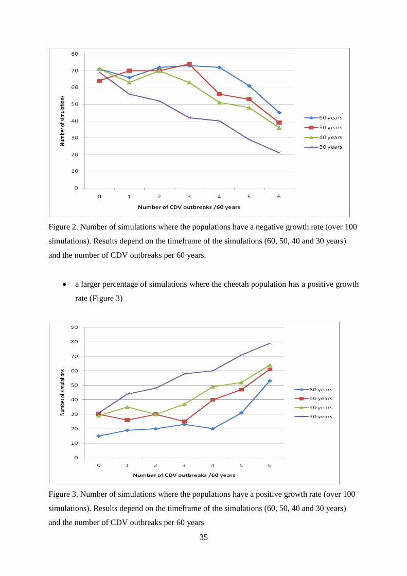
Figure 2. Number of simulations where the populations have a negative growth rate (over 100
simulations). Results depend on the timeframe of the simulations (60, 50, 40 and 30 years)
and the number of CDV outbreaks per 60 years.
a larger percentage of simulations where the cheetah population has a positive growth
rate (Figure 3)
Figure 3. Number of simulations where the populations have a positive growth rate (over 100
simulations). Results depend on the timeframe of the simulations (60, 50, 40 and 30 years)
and the number of CDV outbreaks per 60 years

36
a larger number of cheetahs composing the population after 60 years (Table 12)
Table 12. Average number of cheetahs surviving in the Serengeti plains after 60 years
depending on how the number of CDV outbreaks during the timeframe
Outbreak per 60 years 0 1 2 3 4 5 6
Number of cheetahs alive 54 55 66 68 74 87 110
At the current rate of CDV outbreaks, which seems to be 2 per 60 years, regardless of
the timeframe, every simulation yields a negative average growth rate. This amounts to the
population ultimately going extinct (100 iterations; Figure 1). However, although the average
λ is negative, there are still 20% of the simulations that yield a positive λ over a 60 years
timeframe (Table 11, Figure 3). The percentages of positive growth rates depend on the length
of the simulation timeframe. The shorter the projection is the larger the number of positive λ
e.g. 60 years yields 20% of λ>1 while 30 years yields almost 50% of λ>1 (Table 11). This is
due to the fact that the cheetah is a long-lived species and longer timeframes give a better
overview of the actual population trend. In the event of CDV eradication, there would be a
CDV outbreak rate of 0. Simulations which such a rate yields alarming results; there is little
difference between the average λ obtained for the four timeframes considered (λ is between
0.98 and 0.986, Figure 1.). However, the average numbers of cheetahs still alive after 30 or 60
years in the event of a CDV eradication are different. On average, there are still 130 cheetahs
alive after 30 years while there are only 54 after 60 years. This is once again due to the long-
lived nature of the cheetah and their low reproductive rate.
When the timeframe is 60 years, which is the longest I looked at, the average
population growth rate only barely go over 1 for the largest number of outbreaks: 6 per 60
years. Considering that the current rate in the wild is of 2 per 60 years, such a high CDV
outbreak rate is very unlikely. After a 60 years simulation, the number of cheetahs remaining
in the population depends on how many outbreaks occurred during the 60 years timeframe
(Table 12). There are twice as many remaining cheetahs when there have been 6 outbreaks
than when there has been none. However, the difference between 0 (eradication) and 2
(current rate) outbreaks is only of 12 cheetah individuals.
For the number of simulations where the cheetah population goes extinct before the
end of the timeframe, the pattern is less clear. For a timeframe of 60 years, regardless of the

37
number of outbreaks, there are always at least 2 simulations where the population went
extinct before the sixty year mark. When the outbreak rate is 0, there are as much as 14% of
simulations falling into that category.

38
V/ DISCUSSION
For this project, I hypothesised that the (1) Serengeti plains lion numbers is influenced by
how often a Canine Distemper Virus outbreak occurs and (2) that lion abundance influences
the Serengeti plains cheetah population abundance. To investigate the relationship between
CDV outbreaks, lion abundance and cheetah abundance, I looked at how different outbreak
rates (between 0 and 6 over 60 years) affect the cheetah population growth rate λ. I find that
when the cheetahs are modelled with an influence of lion that is a constant, they have a
positive population growth rate (λ is between 1.03 and 1.01 for timeframes of 30 to 60 years;
results not presented). However, when the lion influence on cheetahs in not a constant (how it
is in nature), the cheetah population growth rate λ can be negative. When using the current
observed CDV outbreak rate (2 outbreaks per 60 years; Packer et al. 2005), I find that
regardless of the simulation timeframe, the average λ is always negative. The situation is the
same for simulations where the cheetah population is modelled with a CDV outbreak rate of 0
(as to simulate eradication). On the other hand, in order for the cheetah population to keep a
positive average growth rate over 60 years, the model suggests the need of at least 6 CDV
outbreaks per 60 years. This is highly unlikely as it would mean one outbreak every 10 years
and the current rate in one every 30 years. However, the actual difference in numbers of
cheetahs remaining in the population after 60 years after 2 or 0 CDV outbreaks is not very
big. For an outbreak rate of 0, on average there are 54 cheetahs left in the population while for
an outbreak rate of 2, there are only 66. For an outbreak rate of 6, the average number of
cheetahs remaining in the population is 110 which still show a decreasing trend. The
simulations results reveal a situation where with the current outbreak rate, the population of
cheetahs in the Serengeti plains hardly survives on the long-term and if the CDV is
eradicated, they may go extinct faster. Protecting the Serengeti lion population is highly
understandable given the potential of a CDV outbreak as illustrated in the Ngorongoro crater
where the lion population has not yet recovered from the 1994 outbreak (Kissui and Packer
2004) However by doing so, conservationist may end up being counter-productive, further
endangering another vulnerable species.
The use of published lion abundance to couple with the cheetah IBM have served to
show that the IBM yields results closer to reality when lion influence is considered to be
variable rather than constant; it goes to prove that there is indeed a link between lion numbers
and cheetah numbers in the plains of the Serengeti NP and therefore reinforce the idea that if
lion abundance were to increase there would be consequences on the cheetah population
survival.

39
As far as the cheetah is concerned, this individual-based model is the most complex
model built so far. Such a model is data hungry and although I have a lot of information on
the cheetahs of the Serengeti plains (from published data and Sarah Durant pers. comm.), I
still had to make assumptions for certain parameters. I could have used a matrix population
model to represent the cheetahs as it requires less data and allows variation in survival and
reproduction as long as individuals are pooled by similar characteristics (age or stage). This
would have led to age (or stage) classes with a very low number of individuals. Considering
that the smaller a population the more important demographic stochasticity is on its long-term
growth rate (Kendall 1998), using a matrix model with average survival rate and reproductive
output across individuals in the same class would lead to a model that performs less well that
one that accounts for individual variability.
There are several limitations to this project. The main one is the poor performance of
the lion matrix population model. The average r-squared between predicted and published
data is 0.20 and the standard deviation is very high (0.19). This shows that the lion model
yields very variable results and isn’t performing very well. It is therefore hard to trust results
obtained from the coupling between the cheetah IBM and the lion matrix population model.
With the current lion model, the simulations tell us that the Serengeti plains cheetah
population is slowly going extinct and that eradicating the CDV will make that happen
slightly faster. However, as there is only a difference of 12 individuals between the numbers
of cheetahs after 60 years, whether 0 or 2 outbreaks occur, it might not make such a big
difference to actually vaccinate lions as far as the cheetahs are concerned. Nonetheless such
conclusions need to be taken cautiously considering that the lion model is not performing
well. The fact that the model is not very good can be explained by the omission of the effect a
pride-organisation can have on population dynamic. Vucetich and Creel (1999) showed that
for animals that have a highly-organised social structure, models that do not take into account
structure-specific ecological interactions are inappropriate. It is the case for the African wild
dog Lycaon pictus, whose individuals are organised in packs. Wild dogs pack structure has a
direct impact their population dynamics through the effect of pack size on foraging and
reproduction successes. Vucetich and Creel (1999) established that they needed to use an
individual-based model mimicking wild dog social structure to draw conclusions on the wild
dog population extinction risk. Like the wild dog, lions are territorial social animals which
are socially organised. Both reproduction and survival are known to be affected by pride
structure. My matrix population model, however, considers the SNP lion population as being
whole where reproduction and survival is not a function of social structure. Therefore, to

40
obtain a better model for lions, there need to incorporation of pride structures. Whitman et al.
(2007) made a spatially explicit individual-based model incorporating prides to look at the
impact of harvesting on the lion population viability. This shows that there should be a
possibility for a better model for lions.
Another limitation comes from the fact that there are several components of each
model that are based on assumptions rather than facts (e.g. the quantitative impact of different
lion abundance on cheetah cubs’ survival, what lion abundance constitutes a high, average or
low one), further reducing the predictive power of those models. Nonetheless, it is very
encouraging that when the cheetah IBM is coupled with the published lion abundance, the r-
squared between predicted and observed cheetah abundance is the highest (r²=0.52); it shows
that the cheetah IBM is quite good at predicting cheetah abundance even if it is on a very
short timeframe (13 years). Finally, each simulation was only run over 100 iterations. This
was due to the time constraint associated with the project but also the capacity of the
computer on which those simulations were performed. Ideally, I would have liked to be able
to perform 1000 iterations for each timeframe/outbreak rates scenario. I believe it would have
led to smoother results for the number of populations that went extinct before reaching the
timeframe deadline and allowed for an estimation of the population probability of extinction
as a function of time.
There are several schools of thoughts in conservation and although there is an
increasing recognition of the constraints of species-based conservation (Mace et al. 2007), it
is still widely practiced. This cheetah-lion case study provides a very good example of one of
the problem related to species-based conservation as opposed to ecosystem-based for
example. Indeed, both lions and cheetahs are acknowledged to be vulnerable on the global
level and remain at relatively low numbers in the Serengeti plains but it seems that one
species protection could impede the other’s survival. By removing one of the natural forms of
control on the lion population (CDV), the cheetah population could be forced to a slightly
faster extinction. On the other hand my results tend to indicate that even at the current rate of
CDV the cheetahs may eventually go extinct and that there would actually be a need for more
CDV outbreaks to favour the cheetah. Although my models have several shortcomings they
hint to the fact that the current situation in the Serengeti plains is not ideal: removing the
CDV might not make much a difference on the cheetahs’ fate but just leaving it as it is now
might be enough to wipe out the cheetah population. Therefore, conservationists might be left
with a choice between two species and several questions: Should the CDV be eradicated to
guarantee lions’ safety since it does not seems to make a big difference on the cheetahs’ fate?

41
Should the lions be assumed have previously recovered from an outbreak and therefore might
not be at a great risk anyway, leaving the CDV as it is? Should an increase of CDV outbreaks
be promoted in order to save the cheetahs while maybe compromising the lions?
This project only begins to answer those questions. It shows that if the CDV is left as
it is now, the lions will continue to prosper (λ>1 from a 30 years to 100 years timeframe;
results not presented) and the cheetahs will slowly move toward their extinction. It is
tempting to remove the CDV as it also affects the bat-eared fox and the spotted hyena, but it
would precipitate the cheetah population towards its end, leaving less time to try to find a
solution for the beloved cat species. At times when there are hundreds of species which need
conservation attention (Millennium Ecosystem Assessment 2005), time to act can be a very
valuable asset against biodiversity loss.
The next step concerning the cheetah population of the Serengeti plains would be to
know exactly how long it will take for the small population to become extinct without
intervention on the CDV (rate of 2 outbreaks) and if the CDV is eradicated (rate of 0). By
quantifying the difference between the two rates, this may give a better idea of how much
time difference a CDV eradication would make on cheetah extinction. Another important step
is to assess if eradication is actually possible. Since the CDV is transmitted from domestic
dogs to wildlife and human population around the Serengeti is increasing (Packer et al. 1999),
one can wonder how efficient would an eradication campaign be. If the dog population keep
increasing or infected dogs are brought from the outside, investing into eradication might not
be cost-efficient. One example where vaccination was not enough to prevent a disease
outbreak is the case of the Ethiopian wolf Canis simensis. The Ethiopian wolf survives in
small pockets of populations and is highly susceptible to rabies (Gotelli and Sillero-Zubiri
1992, Randall et al. 2004). Rabies is transferred to the wolf from the surrounding domestic
dogs’ population. There has been a lot of effort going into dog vaccination but in 2004 an
outbreak was traced back to an infected dog coming from outside the vaccination area
(Randall et al. 2004). If CDV vaccination is deemed feasible and worth doing, to further this
work, how to manage both lions and cheetahs at the same time needs to be investigated, e.g.
timing CDV vaccination interventions when cheetahs are above a certain abundance
threshold. The management would depend on the states of both lion and cheetah populations
when the intervention decision is made. One way to do that is to use stochastic dynamic
programming (SDP); at each time-step SDP compares different management options (e.g.
vaccinate a given number of dogs, vaccinate all the dogs, encourage a CDV outbreak, etc...)
taking into account the current state of the system (e.g. the number of adult cheetahs and adult

42
lions) and decides which management decision is most appropriate to reach the objective (e.g.
maintain at least 100 individuals of each population). The management would therefore be
dynamic and both populations might be managed together.

43
ACKNOWLEDGMENTS
I would like to express my gratitude to my three supervisors, Nathalie Pettorelli, Sarah Durant
and Tim Coulson for giving me the opportunity to carry out this project, being excellent
supervisors and providing me with great advices. I would like to particularly thank Nathalie
for being there every day, guiding me with endless patience and having a constant willingness
to read thesis drafts.
44
REFERENCES
Berry, H., Bush, M., Davidson, B., Forgi, O. & Fox, B. (eds) (1997) Population and Habitat
viability assessment for the Namibian cheetah and lion. Workshop report, IUCN/ SSC
conservation breeding specialist group.
Bro, E., Sarrazin, F., Clobert, J. & Reitz, F. (2000) Demography and the decline of the grey
partridge Perdix perdix in France. Journal of Applied Ecology, 37(3), 432-448.
Caplat, P., Anand, M. & Bauch, C. (2008) Symmetric competition causes population
oscillations in an individual-based model of forest dynamics. Ecological Modelling,
211(3-4), 491-500.
Caro, T. M. (1987) Cheetah mothers vigilance- looking out for prey or for predators.
Behavioral Ecology and Sociobiology, 20(5), 351-361.
Caro, T. M. (1994) Cheetahs of the Serengeti Plains. Chicago, The University of Chicago.
Caswell, H. (2001) Matrix population models. Sunderland, Sinauer Associates.
Caswell, H. (2009) Sensitivity and elasticity of density-dependent population models. Journal
of Difference Equations and Applications, 15(4), 349-369.
Carpenter, M. A., Appel, M. J. G., Roelke-Parker, M. E., Munson, L., Hofer, H., East, M.
&O'Brien, S. J. (1998) Genetic characterization of canine distemper virus in Serengeti
carnivores. Veterinary Immunology and Immunopathology, 65(2-4), 259-266.
Cleaveland, S., Mlengeya, T., Kaare, M., Haydon, D., Lembo, T., Laurenson, M. K. &
Packer, C. (2003) The conservation relevance of epidemiological research into
carnivore viral diseases in the Serengeti. Conservation Biology, 21 (3), 612-622.
Clutton-Brock, T. H. (1988) Reproduction success. Chicago, University of Chicago Press.
Courchamp, F., Langlais, M. & Suhigara, G. (1999) Cats protecting birds: modelling the
mesopredator release effect. Journal of Animal Ecology, 68, 282-292.

45
Crooks, K. R., Sanjayan, M. A. & Doak, D. F. (1998) New insight on cheetah conservation
through demographic modeling. Conservation Biology, 12(4), 889-895.
Cropper, W. P. & Loudermilk, E. L. (2006) The interaction of seedling density dependence
and fire in a matrix population model of longleaf pine (Pinus palustris). Ecological
Modelling, 198(3-4), 487-494.
De Roos, A. M., Persson, L. &McCauley, E. (2003) The influence of size-dependent life-
history traits on the structure and dynamics of populations and communities. Ecology
Letters, 6(5), 473-487.
Durant, S. M. (1991) Individual variation and dynamics of small population: implications for
conservation and management. PhD thesis. Cambridge University, UK.
Durant, S. M., Bashir, S., Maddox, T. & Laurenson, M. K. (2007) Relating long-term studies
to conservation practice: the case of the Serengeti Cheetah Project. Conservation
Biology, 21(3), 602-611.
Durant, S. M., Dickman , A. J., Maddox, T., Waweru, M., & Pettorelli, N. in press Past,
present and future of the cheetah in Tanzania: their behavioural ecology and
conservation. In: Macdonald, DW & AJ Loveridge (eds). Biology and Conservation of
Wild Felids. Oxford University Press.
Eberhardt, L. L. (2002) A paradigm for population analysis of long-lived vertebrates.
Ecology, 83(10), 2841-2854.
Fowler, C. W. (1981) Density dependence as related to life-history strategy. Ecology, 62(3),
602-610.
Foxcroft, L. C., Rouget, M. & Richardson, D. M. (2007) Risk Assessment of riparian plant
invasions into protected areas. Conservation Biology, 21(2), 412-421.
Gotelli, D. & Sillero-Zubiri, C. (1992) The Ethiopian wolf- an endangered endemic canid.
Oryx, 26(4), 205-214.
Grenier, M. B., McDonald, D. B. & Buskirk, S. W. (2007) Rapid population growth of a
critically endangered carnivore. Science, 317(5839), 779-779.
46
Grimm, V. (1999) Ten years of individual-based modelling in ecology: what have we learned
and what could we learn in the future? Ecological Modelling, 115(2-3), 129-148.
Grimm, V. & Railsback, S. F. (2005) Individual-based modelling and ecology. Priceton
University Press.
Grimm, V., Revilla, E., Berger, U., Jeltsch, F., Mooij, W. M., Railsback, S. F., Thulke, H. H.,
Weiner, J., Wiegand, T. & DeAngelis, D. L. (2005) Pattern-oriented modeling of
agent-based complex systems: Lessons from ecology. Science, 310(5750), 987-991.
Hanby, J. P., Bygott, J. D. & Packer, C. (1995) Ecology, demography and behaviour of lions
in two contrasting habitats: Ngorongoro crater and Serengeti plains. In: Sinclair, A. R.
E. & Arcese, P. (eds). Serengeti II. Dynamics, management and conservation of an
ecosystem. The University of Chicago Press.
Hamilton, A., Cunningham, A., Byarugaba, D. & Kayanja, F. (2000) Conservation in a region
of political instability: Bwindi Impenetrable forest, Uganda. Conservation Biology,
14(6), 1772-1725.
Holt, R. D. & Pickering, J. (1985) Infectious disease and species coexistence. A model of
Lokta-Volterra form. American Naturalist, 126(2), 196-211.
Huston, M., Deangelis, D. & Post, W. (1988) New computer models unify ecological theory.
Computer simulations show that many ecological patters can be explained by
interactions among individual organisms. Bioscience, 38(10), 682-691.
IUCN (2009) IUCN Red List of Threatened Species. Version 2009.1. <www.iucnredlist.org>.
Downloaded on 10 July 2009.
Kelly, M. J. & Durant, S. M. (2000) Viability of the Serengeti cheetah population.
Conservation Biology, 14(3), 786-797.
Kendall, B. E. (1998) Estimating the magnitude of environmental stochasticity in survivorship
data. Ecological Applications, 8(1), 184-193.

47
Kissui, B. M. & Packer, C. (2004) Top-down population regulation of a top predator: lions in
the Ngorongoro Crater. Proceedings of the Royal Society of London Series B-
Biological Sciences, 271(1550), 1867-1874.
Lacy, R. C., Borbat, M. & Pollack, J. P. (2005) Vortex: A stochastic simulation of the
extinction process. Brookfield, IL, Chicago Zoological Society.
Laurenson, M. K. (1994) High juvenile mortality in cheetahs (Acinonyx jubatus) and its
consequences for maternal care. Journal of Zoology, 234, 387-408.
Laurenson, M. K. (1995) Implications of high offspring mortality for cheetah population
dynamics. In: Sinclair, A. R. E. & Arcese, P. (eds). Serengeti II. Dynamics,
management and conservation of an ecosystem. The University of Chicago Press.
Le Maitre, D. C., Krug, R. M., Hoffmann, J. H., Goydon, A. J. & Mgidi, T. N. (2008) Hakea
sericea: Development of a model of the impacts of biological control on population
dynamics and rates of spread of an invasive species. Ecological Modelling, 212(3-4),
342-358.
Lee, T. M. & Jetz, W. (2008) Future battlegrounds for conservation under global change.
Proceedings of the Royal Society B-Biological Sciences, 275(1640), 1261-1270.
Levin, S. A. (1970) Community equilibria and stability, and an extension of competitive
exclusion principle. American Naturalist, 104(939), 413-423.
Mace, G. M., Possingham, H. P. & Leader-William, N. (2007) Prioritizing choices in
conservation. In McDonald, D. & Service, K. (eds) Key topics in conservation
biology. Oxford, Blackwell Publishing Ltd.
Millennium Ecosystem Assessment (2005) Ecosystems and Human Well-being: Biodiversity
Synthesis. World Resources Institute, Washington, DC.
Moreno, R. S., Kays, R.W. & Samudio, R. (2006) Competitive release in diets of ocelot
(Leopardus pardalis) and puma (Puma concolor) after jaguar (Panthera onca) decline.
Journal of mammology, 87, 808–816.

48
Murray, D. L., Kapke, C. A., Evermann, J. F. & Fuller, T. K. (1999) Infectious disease and
the conservation of free-ranging large carnivores. Animal Conservation, 2(4), 241-
254.
Nehrbass, N. & Winkler, E. (2007) Is the Giant Hogweed still a threat? An individual-based
modelling approach for local invasion dynamics of Heracleum mantegazzianum.
Ecological Modelling, 201(3-4), 377-384.
Obrien, S. J., Roelke, M. E., Marker, L., Newman, A., Winkler, C. A., Meltzer, D., Colly, L.,
Evermann, J. F., Bush, M. & Wildt, D. E. (1985) Genetic basis for species
vulnerability in the cheetah. Science, 227(4693), 1428-1434.
Oconnor, T. G. (1993) The influence of rainfall and grazing on the demography of some
African savanna grasses. A matrix modeling approach. Journal of Applied Ecology,
30(1), 119-132.
Ogutu, J. O. & Dublin, H. T. (2002) Demography of lions in relation to prey and habitat in the
Maasai Mara National Reserve, Kenya. African Journal of Ecology, 40(2), 120-129.
Packer, C., Altizer, S., Appel, M., Brown, E., Martenson, J., O'Brien, S. J., Roelke-Parker, M.,
Hofmann-Lehmann, R. & Lutz, H. (1999) Viruses of the Serengeti: patterns of
infection and mortality in African lions', Journal of Animal Ecology, 68(6), 1161-
1178.
Packer, C., Pusey, A. & Eberly, L. E. (2001) Egalitarianism in female African lions. Science,
293, 690-693.
Packer, C., Hilborn, R., Mosser, A., Kissui, B., Borner, M., Hopcraft, G., Wilmshurst, J.,
Mduma, S. &Sinclair, A. R. E. (2005) Ecological change, group territoriality, and
population dynamics in Serengeti lions. Science, 307(5708), 390-393.
Pettorelli, N. & Durant, S. (2007a) Family effects on early survival and variance in long-term
reproductive success of female cheetahs. Journal of Animal Ecology, 76, 908-914.
Pettorelli, N. & Durant, S. (2007b) Longevity in cheetahs: the key to success? Oikos, 116,
1879-1886.

49
Possingham, H. P. (2002) Ecological triage. Nature Australia, 27, 84.
Randall, D. A., Williams, S. D., Kuzmin, I. V., Rupprecht, C. E., Tallents, L. A., Tefera, Z.,
Argaw, K., SHiferew, F., Knobel, D. L., Sillero-Zubiri, C. & Laurenson, M. K. (2004)
Rabies in Ethipian wolves. Emerging infectious diseases, 10(12), 2214-2217.
Reuter, H. (2005) Community processes as emergent properties: Modelling multilevel
interaction in small mammals communities. Ecological Modelling, 186(4), 427-446.
Reuter, H., Holker, F., Middelhoff, U., Jopp, F., Eschenbach, C. & Breckling, B. (2005) The
concepts of emergent and collective properties in individual-based models - Summary
and outlook of the Bornhoved case studies. Ecological Modelling, 186(4), 489-501.
Ritchie, E. G. & Johnson, C. N. (2009) Predator interactions, mesopredator release and
biodiversity conservation. Ecology letters, 12, 982-998.
Rockwood, L. L. (2006) Introduction to population biology. Oxford, Blackwell Publishing.
Rodrigues, A.S.L., Andelman, S.J., Bakarr, M.I., Boitani, L., Brooks, T.M., Cowling, R.M.,
Fishpool, L.D.C., da Fonseca, G.A.B., Gaston, K.J., Hoffmann, M., Long, J.S.,
Marquet, P.A., Pilgrim, J.D., Pressey, R.L., Schipper, J., Sechrest, W., Stuart, S.N.,
Underhill, L.G., Waller, R.W., Watts, M.E.J. & Yan, X. (2004) Effectiveness of the
global protected area network in representing species diversity. Nature 428,
640–643.
RoelkeParker, M. E., Munson, L., Packer, C., Kock, R., Cleaveland, S., Carpenter, M.,
Obrien, S. J., Pospischil, A., HofmannLehmann, R., Lutz, H., Mwamengele, G. L. M.,
Mgasa, M. N., Machange, G. A., Summers, B. A. & Appel, M. J. G. (1996) A canine
distemper virus epidemic in Serengeti lions (Panthera leo). Nature, 379(6564), 441-
445.
Scheel, D. & Packer, C. (1995) Variation in predation by lions: tracking a movable feast. In:
Sinclair, A. R. E. & Arcese, P. (eds). Serengeti II. Dynamics, management and
conservation of an ecosystem. Chicago, The University of Chicago Press.
Scott, B. E., Marteinsdottir, G., Begg, G. A., Wright, P. J. & Kjesbu, O. S. (2006) Effects of
population size/age structure, condition and temporal dynamics of spawning on

50
reproductive output in Atlantic cod (Gadus morhua). Ecological Modelling, 191(3-4),
383-415.
Shaffer, M. (1987) Minimum viable population coping with uncertainty. In Soulé, M. E. (ed).
Viable populations for conservation. Cambridge, Cambridge University Press.
Sinclair, A. R. E. (1995) Serengeti past and present. In: Sinclair, A. R. E. & Arcese, P. (eds).
Serengeti II. Dynamics, management and conservation of an ecosystem. The
University of Chicago Press.
Towns, D. R. & Broome, K. G. (2003) From small Maria to massive Campbell: forty years of
rat eradication from New Zealand islands. New Zealand Journal of Zoology, 30(4),
377-398.
Vucetich, J. A. & Creel, S. (1999) Ecological interactions, social organization and extinction
risk in African wild dogs. Conservation Biology, 13(5), 1172-1182.
Walters, J. R., Crowder, L. B. & Priddy, J. A. (2002) Population viability analysis for red-
cockaded woodpeckers using an individual-based model. Ecological Applications,
12(1), 249-260.
Williams, B. K., Nichols, J. D. & Conroy, M. J. (2001) Analysis and management of animal
populations. San Diego, Academic Press.
Whitman, K. L., Starfield, A. M., Quadling, H. & Packer, C. (2007) Modelling the effect of
trophy selection and environmental disturbances on a simulated population of African
lions. Conservation Biology, 21(3), 591-601.
Woodroffe, R. (1999) Managing disease threats to wild mammals. Animal Conservation, 2(3),
185-193.