canadian agrifood export performance and the growth potential...

CANADIAN AGRIFOOD EXPORT PERFORMANCE AND THE GROWTH

POTENTIAL OF THE BRICs AND NEXT-11.

CATPRN Working Paper 2012-05 July 2012

Alexander P. Cairns

and Karl D. Meilke

Department of Food, Agricultural and Resource Economics University of Guelph

http://www.catrade.org

Funding for this project was provided by the Canadian Agricultural Trade Policy and Competitiveness Research Network (CATPRN) who in turn is funded by Agriculture and Agri-Food Canada. The views in this paper are those of the authors and should not be attributed to the funding agency.

Abstract

In 2011, the Canadian Agrifood Policy Institute released an report highlighting theimportance of the agrifood sector to the economy and concluded by stating the needfor Canada to double the dollar value of agrifood exports to ensure the viability of thesystem. This paper seeks to estimate Engel elasticities faced by Canada and four othermajor agrifood exporter groups for two groups of emerging economies known as theNext-11 and the BRICs, and to forecast the value of agrifood exports to 2017. Thefindings suggest that despite the relatively low Engel elasticities for agrifood importsfaced by Canada, it could sell an additional $3.65 billion in agrifood products to theNext-11 and BRICs by 2017.

Keywords: Agrifood Trade; Import Demand Model; BRICs; Next-11; Engel Elasticities.

Introduction

In 2011, the Canadian Agrifood Policy Institute (CAPI) released a report assessing the state

of Canada’s agrifood sector. The report highlighted the importance of the agrifood sector to

the Canadian economy – noting that the sector employs 1 in 8 Canadians – and concluded

by arguing for the need to double the value of exports to $75 billion (in Canadian dollars)

by 2025 to insure the viability of the sector (CAPI, 2011). If Canada is to achieve CAPI’s

stated objective, it is important for firms and policy-makers to identify those foreign markets

where increases in import demand, arising from economic growth, is most likely.

The reliance of Canadian agriculture on trade is notable with roughly 80% of annual

farm cash receipts derived from export-dependent commodities (CAFTA, 2008). In 2008,

the value of Canadian agrifood exports totalled $36.4 billion rendering it the fourth largest

exporter after the EU ($426.8 billion), the United States ($104.1 billion) and Brazil ($49.6

billion) (United Nations, 2010).1 However, Canada’s share of the global agrifood export

market has remained stagnant at roughly 3.7% over the last two decades (United Nations,

2010) (figure 1), and heavily contingent on access to US markets. Exports to the US have

grown consistently since the implementation of the Canada- United States trade agreement

(CUSTA) in 1989 – the predecessor to the North American Free Trade Agreement (NAFTA)

– and on average accounted for 63 percent of our agrifood exports between 2000 and 2009

(United Nations, 2010), but an over-reliance on the US for export opportunities could leave

Canadian agrifood exporters vulnerable to fluctuations in the Canada-US exchange rate as

well as any economic downturn that dampens the US demand for imports. Furthermore, the

gains from CUSTA, and it’s successor NAFTA, are largely achieved as the liberalization of

trade barriers and the harmonization of regulations and institutions is largely completed.

Ignoring the role of prices, the magnitude of any increase in imports is largely contingent

1All values in US dollars unless otherwise noted.

2

*Source: Data obtained from United Nations (2010)

Figure 1: Canada’s Agrifood Exports, 1995-2010

on: population growth, income growth and the responsiveness of per capita expenditure to

increases in income.2 Cranfield et al. (2002) estimated di↵erences in expenditure elasticities

across countries at various stages of development, finding that Engel elasticities for food are

notably larger for developing nations relative to industrialized countries.3 This suggests that

increases in absolute expenditure on food are likely to be greatest in emerging markets where

population and income growth are projected to be the largest.

Wilson and Purushothaman (2003) and Wilson and Stupnytska (2007) identified two

groups of emerging economies where rapid GDP growth was expected based on their large

populations, the BRICs and the Next-11 (N-11), suggesting that projected economic growth

2Prices also play a major role in determining the magnitude of demand for all commodities. This studywill ignore this obvious fact, as its focus is predominantly on the role of income growth on expenditure.

3Engel elasticities indicate the responsiveness of expenditure to income growth – e.g. a one percentgrowth in income leads to a x% growth in expenditure. Thus, they parallel income elasticities but measurethe responsiveness of expenditure rather than income.

3

*Source: Data obtained from IMF World Economic Outlook Database (2012)

Figure 2: Average GDP growth rate, 2000-2017

in several member countries could result in their GDPs surpassing several of the current

G7 members. Assuming the extrapolated population and income growth foreseen by Wilson

and Purushothaman (2003) and Wilson and Stupnytska (2007) comes to fruition (figure 2),

these two groups of countries could represent new sources of demand for Canadian agrifood

products. However, even if income growth occurs, any increase in import demand is con-

tingent on how responsive expenditure on agrifood imports is to income. This study seeks

to estimate whether Engel elasticities faced by Canadian agrifood exports di↵ers from other

major agrifood exporters for the BRICs4 and ’Next-11’5 and if their import profiles di↵er

from other low, middle or high income countries.

4BRIC members: Brazil, Russia, India, China.5N-11 members: Bangladesh, Egypt, Indonesia, Iran, Mexico, Nigeria, Pakistan, Philippines, South Ko-

rea, Turkey and Vietnam.

4

The Model

This study follows Haq and Meilke (2009a) and Cairns and Meilke (2012) in its use of

Hallak’s (2006) model, which assumes a two stage budgeting procedure. It is assumed that

a representative consumer possesses an additively separable utility function implying that

the utility gained from the consumption of imported agrifood products is di↵erentiable from

all other products (Cairns and Meilke, 2012; Hallak, 2006; Haq and Meilke, 2009a). It

also adopts the conventional Armington assumption, which argues that imported agrifood

products are di↵erentiated by exporter, and therefore, not perfect substitutes for each other.

In the first stage, the consumer exogenously allocates their consumption expenditures

between imported agrifood products and all other goods. In the second stage, the rep-

resentative consumer maximizes a CES utility function with Dixit-Stiglitz preferences by

purchasing imported products from various exporters subject to the total proportion of in-

come allocated to importable agrifood products in year t (equation 1) (Cairns and Meilke,

2012; Hallak, 2006; Haq and Meilke, 2009a,b):

Ma

x

x U

it

=JX

j=1

(x⇢

ijt

)1⇢ (1)

s.t. E

it

=JX

j=1

x

ijt

p

ijt

where x

ijt

and p

ijt

are the quantity of agrifood demanded from exporter j by the represen-

tative consumer in country i and the price in the importing country of the agrifood product

from country j in time t and P

ijt

represents an index of prices faced by importer i for ex-

porters j where j = 1 . . . J . The utility function in equation 1 is subject to a substitution

parameter (⇢), which accounts for the propensity to substitute between various exporters.

The substitution parameter has a lower asymptote of zero in order to prevent the possibility

5

that imports from di↵erent exporters are consumed in fixed proportions.6 This is a realistic

constraint, as convention dictates that an exporter’s share of a country’s imports typical

varies from year to year. Its upper bound is constrained to be less than one to ensure strict

concavity of the utility function and to eliminate the possibility of linearity.7

Optimization of the constrained maximization problem produces the Marshallian demand

function for a representative consumer (Cairns and Meilke, 2012; Haq and Meilke, 2009a):

x

ijt

=(p

ijt

)1

(⇢�1)

PJ

j=1 P

⇢(⇢�1)

ijt

E

ijt

(2)

From this demand function it is easy to generate a function for the per capita expenditure

on imports in country i from exporter j by multiplying equation 2 by the price of the good

in the importing country (pijt

) to get:

p

ijt

x

ijt

=p

⇢(⇢�1)

ijtPJ

j=1(Pijt

)⇢

(⇢�1)

E

it

(3)

It is assumed here that the price of an imported good from exporter j is a function of

the exporter’s cost of production and the trade costs an importer faces when trading with

the specific exporter, therefore let pijt

= p

jt

t

it

.8 For notational simplicity, let the elasticity

of substitution between agrifood importers be a function of the substitution parameter as

represented by � = 11�⇢

. Incorporating these changes into equation 3 and defining the per

6As ⇢ ! 0 then the utility function begins to mimic a Leontief utility function, which would imply thatimported agrifood products are perfect complements.

7Imposing strict concavity of the utility function indicates that it is also quasiconcave and therefore theindi↵erence curves will be strictly convex to the origin. Strict convexity of the indi↵erence curve implies thatthe consumer prefers variety they enjoy consuming imports from several exporters. This dismisses the notionof perfect substitutes which would suggest that the importing country imports food products from singlesource. Thus, if ⇢ = 1 then the goods are perfect substitutes since equation 1 simplifies to Uit =

PJj=1 xjt

and the consumer would be indi↵erent between the source of the imported agrifood products8Note that tijt must be greater than 1, otherwise it would imply there there are no transaction costs of

engaging in international trade, which transitively implies that a given country is trading with itself.

6

capita expenditure on agrifood imports (from exporter j) as imp

ijt

= p

ijt

x

ijt

gives:

imp

ijt

=(p

jt

t

ijt

)1��

PJ

j=1(Pjt

T

ijt

)1��

E

it

(4)

where Pjt

T

ijt

is an index of prices faced by consumers in the importing country (i) in period

t.

The empirical model is obtained from the equation 4 by taking the natural logarithm of

both sides of equation 4, substituting in several variables representing trade costs for tijt

and

adding a stochastic error term to get (Cairns and Meilke, 2012; Haq and Meilke, 2009a,b):

lnImp

ijt

=

i

+

j

+

t

+ �1lnIncome

it

+ �2lnDist

ij

+ �3Adjij + �4Langij

+ �5Colony

ij

+ �6PTA

ijt

+ µ

ijt

(5)

Following convention (in the literature on the gravity model), equation 5 contains vari-

ables proxying the cost of engaging in trade with a particular exporter (t in equation 4).

Here dummy variables are set equal to one if the importer shares a common o�cial lan-

guage, is adjacent to the exporter, had a common colonizer, and/or if a preferential trade

agreement or custom union exists between the trading partners, and zero otherwise. The

distance variable is the natural logarithm of the distance between the “economic centres” of

a country pair. It is calculated by first taking the average distance between economic centres

of the exporter (importer) weighted by their respective shares of the country’s population

and then using these estimates to measure the distance between the trading partners (Head

and Mayer, 2002; Mayer and Zignago, 2005).

7

Empirical Considerations

Several articles dealing with trade flows have discussed the proper estimation of the gravity

model (e.g. Anderson and van Wincoop (2003), Matyas (1997), Egger (2000), Haq, Meilke,

and Cranfield (2010)). Most recently, a study by Baier and Bergstrand (2007) suggests that

previous attempts to estimation of the average treatment e↵ects (the average e↵ect on trade)

of a preferential trade agreement or customs union su↵ers from endogeneity bias. Baier and

Bergstrand (2007) state that endogeneity arises for three reasons: omitted variable bias,

measurement error and simulateneity. Baier and Bergstrand (2007) claim that omitted vari-

able bias could arise from the exclusion of relevant policy variables which act as determinants

of the formation of a PTA (Baier and Bergstrand, 2004), while measurement error results

from the use of a binary dummy variable to capture the e↵ect of a heterogeneous group of

PTAs which can di↵er substantially in scope and coverage. Simultaneity bias can arise due

to the ambiguity of the direction of causation between trade flows and trade agreements —

are trade agreements negotiated to increase trade flows; or are they used to institutionalize

already established relationships between trading partners (Baier and Bergstrand, 2007)?

Baier and Bergstrand (2007) conclude that the endogeneity bias encountered in using panel

data can be corrected through the use of a fixed e↵ects estimator (an approach originally

advocated by Egger (2000)).

Endogeneity bias presents a potential problem, that we handle through the inclusion of

exporter, importer and year fixed e↵ects (as advocated by Matyas (1997) and Anderson and

van Wincoop (2003)) to account for country heterogeneity – which would also capture the

e↵ect of any policy that could cause omitted variable bias. Bias caused by the endogeniety of

PTAs and trade is an unlikely issue for us as agricultural trade is a small proportion of total

trade. In contrast, we feel that zero trade flows (corresponding to a non-random sample),

which may introduce sample selection bias into the model, is a more pertinent issue.

8

Due to the use of a log-linear functional form the presence of zero trade flows presents

a dilemma. Zero trade flows can arise for two reasons. First, countries may not engage in

trade with each other, not every importer trades with every exporter - e.g. a given product

may only be produced by specific exporters. Second, the data may be missing. In either

case, simply dropping observations with zero trade flows would result in biased parameter

estimates9; a bias which Heckman (1976) identified as a case of omitted variable bias in

his seminal paper, which can be corrected for through the use of his two–stage estimation

procedure. This study takes the advice of Puhani (2000) and Dow and Norton (2003), and

adopts the (full–information) maximum likelihood estimator as it is more e�cient, relative

to the two-step (limited information maximum likelihood) estimator originally suggested by

Heckman (1976), to account for the presence of zero trade flows.

The Heckman model accounts for the sample selection issue through the inclusion of the

inverse mills ratio, and therefore the marginal e↵ects must be extracted from the parameter

estimates. Derivation of the marginal e↵ects is contingent on what assumptions are made

regarding the origin of the zero trade flows. If the zero trade flows arise due to the absence

of trade between a given country pair then they represent actual outcomes and require the

derivation of conditional marginal e↵ects (Dow and Norton, 2003). In contrast, if the zero

is due to missing data, then they are indicative of potential outcomes, or latent outcomes,

and calculation of the unconditional marginal e↵ects is required. Some have argued that a

two-part model is preferable to the Heckman model if the zeros represent actual outcomes

(Dow and Norton, 2003; Leung and Yu, 1996; Puhani, 2000). However, due to the inclu-

sion of numerous developing countries in our sample, it is unlikely that all zeros represent

actual outcomes; it is more plausible that some zeros represent missing data. Therefore, the

Heckman selection model will be employed as it permits the derivation of marginal e↵ects

for both actual and potential outcomes.

9One cannot take the log of zero which has led some researchers to simply drop them from the data set.

9

We also estimate the model using, what we call, subsample OLS which simply means

that we drop all non-positive trade flows and estimate using OLS. This was done to test the

extent of sample selection bias and to examine the robustness of our findings.

Data

This study uses a sample consisting of 47,360 bilateral agrifood trade flows for 40 major

agrifood exporters to 75 importers between 1995-2010. Exporters were included if they were

a member of the EU-27 and/or if they account for, on average, at least 1% of the value of

global agrifood exports over the sample period10, while criteria for inclusion as an importer

required that the country represents at least an average of 0.1% of the value of global agrifood

imports and/or if the country is a member of either the EU-27, BRICs or N-11.11 The

dependent variable is the natural logarithm of the real per capita expenditure on agrifood

imports – the annual value of agrifood imports obtained from UN Comtrade divided by the

IMF population estimates. We define agrifood according to the World Integrated Trading

Solution classification of food at the SITC revision 3 level, which includes: 0 – food and

live animals; 1 – beverages and tobacco; 22 – oilseeds/oil fruits; and 4 – animal/vegetable

oils/fat/wax.

Income is proxied by real per capita GDP obtained from the IMF’s World Economic

Outlook Database. The common colonizer, adjacency, shared o�cial language and distance

variables were retrieved from the CEPII’s gravity dataset available on their website. The

10Exporter include (from largest exporter to smallest): all members of the EU-27, US, Brazil, Canada,China, Argentina, Australia, Thailand, Mexico, Malaysia, Indonesia, New Zealand, India, Chile, and Turkey.

11Importers: from the low income ranking - Cuba, Ghana, Iraq and the Sudan; from the middle income- Algeria, Chile, Columbia, Dominican Republic, Ecuador, Guatemala, Jamaica, Libya, Malaysia, Morocco,Peru, Saudi Arabia, South Africa, Sri Lanka, Thailand, Trinidad and Tobago, Tunisia and Venezuela; fromthe high income ranking - Australia, Canada, EU-27, Hong Kong, Japan, New Zealand, Norway, Singapore,Switzerland, Taiwan, United Arab Emirates, and the United States; from the BRICs - Brazil, Russia, India,China; from the N-11 - Bangladesh, Egypt, Indonesia, Iran, Mexico, Nigeria, Pakistan, Philippines, SouthKorea, Turkey and Vietnam; and, again all members of the EU-27.

10

PTA dummy variable was constructed from a list of regional trade agreements on the WTO’s

website (WTO, 2009) and only includes preferential trade agreements and custom unions

due to the ambiguous coverage of most partial scope agreements. All monetary variable are

deflated using the IMF implicit price deflator (base year = 2005).

Results

We estimate the Engel elasticities faced by five major exporters/exporter groups: Australia,

Canada, the EU, the US and a hypothetical group representing the remaining 11 exporters

included in the sample (ROW). All current members of the European Union (EU) are aggre-

gated and treated as a single exporter; despite the fact that EU membership increases over

the sample period – i.e., in 1995, there were only 15 members and the current EU-27 came

into existence in 2007 with the ascension of Bulgaria and Romania.12 Due to the Canadian-

centric approach of this study, these exporter groups were chosen in order to contrast the

elasticities faced by the two largest agrifood exporters (US and the EU), and Australia, a

country which shares many characteristics with Canada (including the general composition

of their agricultural exports).

Due to the use of panel data, the Bruesch-Pagan tests for heteroskedasticity andWooldridge’s

test for serial correlation (Wooldridge, 2002) were preformed and revealed that both are

present. Due to the ambiguous nature of the forms of heteroskedasticity and autocorrela-

tion, all regressions were estimated with robust standard errors to correct for this.

Exporter, importer and year fixed e↵ects were included to account for country and year

heterogeneity (Matyas, 1997). As discussed by Anderson and van Wincoop (2003) these

12Although the composition of the EU changes over our sample period, we include all members of theEU-27 in the EU exporter group throughout the sample. This was done for simplicity, as interpretationof the coe�cient estimates would be ambiguous if we opted to define the group according to the year eachmember joined. Furthermore, the latter approach would have led to the composition of the ROW groupchanging and cross comparison of the estimated Engel elasticities di�cult.

11

fixed e↵ects also control for the omission of a price variable in the empirical model.13 A

likelihood ratio test confirms that inclusion of fixed e↵ects significantly improves the fit of

the model, while a Wald test for joint equality rejected the hypothesis that the joint e↵ect

of the importer, exporter and year fixed e↵ects are zero. Thus, it can be concluded that

omitting the fixed e↵ects would have biased the parameter estimates. The downfall of using

fixed e↵ects to proxy price terms is that their interpretation is highly ambiguous, as the

source of the country heterogeneity is unclear; and the marginal e↵ect of an increase (or

decrease) in price is indistinguishable from other sources of heterogeneity.

Finally, a t-test for sample selection bias was preformed on the estimated coe�cients of

the inverse mills ratio (⇢ and ln�). In both specifications, the t–test identified that sample

selection bias was present due to the presence of zero trade flows (table 4 and 6). For

simplicity, the remaining discussion of the results will focus on the estimated parameters

from the unconditional marginal e↵ect due to the fact that sample selection bias is present

and the fact that the unconditional marginal e↵ects represents the combined e↵ect of both

the increase in the expenditure on imported agrifood products given an increase in income in

countries that trade and the increased probability of a country importing agrifood products.

Specification 1

The first specification interacts the five exporter groups with five importing country groups

and income, resulting in 25 individual Engel elasticities. To estimate the Engel elasticities for

imported agrifood products, dummy variables are generated for the five mutually exclusive

importer groups: the BRICs, the N-11, and low, middle and high income countries and

interacted with the natural logarithm of income (proxied by the natural logarithm of GDP

13Anderson and van Wincoop (2003) use the term “multilateral resistance terms” in their discussion ofprice e↵ects on trade flows. Essentially, the latter term refers to the di↵erence between the cost of tradingwith a given exporter relative to the average price of engaging in trade with all other exporters (Andersonand van Wincoop, 2003).

12

per capita). If an importer is a member of the BRICs or N-11 they are excluded from the

other income groups. Non-N-11 and non-BRIC countries included in the sample are classified

according to the World Banks income groups. The composition of each income group may

vary annually as some countries may experience enough per capita income growth (loss) to

warrant a graduation (demotion) to another group. To estimate the Engel elasticities faced

by each exporter, dummy variables identifying each exporter (group) are generated then

interacted with the importer group dummy variable and the natural logarithm of income.

The results from this estimation are in table 4.

As can be seen in table 4 the common language, common colonizer, adjacency and dis-

tance variables all have the expected signs and are statistically significant at the 0.01% level.

The PTA variable indicates that it is statistically significant and possesses the expected sign,

however its magnitude, suggesting that, on average, the establishment of a PTA only garners

a 10 percent increase in agrifood imports, implies a substantially lower e↵ect on agricultural

trade than is conventionally reported in the literature (e.g. Grant and Lambert (2008); Haq

and Meilke (2009a,b)).14

All group Engel elasticities are positive and statistically significant suggesting that income

has a positive e↵ect on per capita expenditure on agrifood imports across all exporters. Wald

tests for joint equality of the Engel elasticities confirm that the magnitude of the elasticities

for each importer group varies by exporter (column e, table 5).

Table 1 ranks the exporters according to the size of the income elasticity they face (from

highest to lowest), by importer group. Table 1 reveals that Canada and Australia face lower

income elasticities relative to the other exporters (US, EU-27 and ROW). For low, middle

and high income countries the EU-27 has the highest elasticity, following by ROW and the

14The much lower estimates of the value of a PTA contained in this study – in comparison to those inGrant and Lambert (2008) and Cairns and Meilke (2012) – are of concern and will be the subject of furtherresearch. However, we speculate that the larger the number of countries included in the sample the lowerthe estimated e↵ect of a PTA. We speculate that the e↵ect of a PTA on bilateral trade flows involving oneor two small countries have a much smaller e↵ect on trade than those including one or two large countries.

13

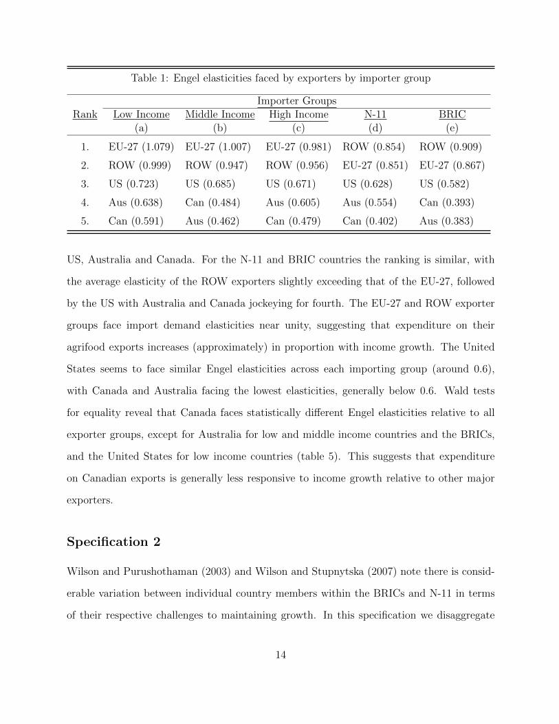
Table 1: Engel elasticities faced by exporters by importer group

Importer GroupsRank Low Income Middle Income High Income N-11 BRIC

(a) (b) (c) (d) (e)

1. EU-27 (1.079) EU-27 (1.007) EU-27 (0.981) ROW (0.854) ROW (0.909)

2. ROW (0.999) ROW (0.947) ROW (0.956) EU-27 (0.851) EU-27 (0.867)

3. US (0.723) US (0.685) US (0.671) US (0.628) US (0.582)

4. Aus (0.638) Can (0.484) Aus (0.605) Aus (0.554) Can (0.393)

5. Can (0.591) Aus (0.462) Can (0.479) Can (0.402) Aus (0.383)

US, Australia and Canada. For the N-11 and BRIC countries the ranking is similar, with

the average elasticity of the ROW exporters slightly exceeding that of the EU-27, followed

by the US with Australia and Canada jockeying for fourth. The EU-27 and ROW exporter

groups face import demand elasticities near unity, suggesting that expenditure on their

agrifood exports increases (approximately) in proportion with income growth. The United

States seems to face similar Engel elasticities across each importing group (around 0.6),

with Canada and Australia facing the lowest elasticities, generally below 0.6. Wald tests

for equality reveal that Canada faces statistically di↵erent Engel elasticities relative to all

exporter groups, except for Australia for low and middle income countries and the BRICs,

and the United States for low income countries (table 5). This suggests that expenditure

on Canadian exports is generally less responsive to income growth relative to other major

exporters.

Specification 2

Wilson and Purushothaman (2003) and Wilson and Stupnytska (2007) note there is consid-

erable variation between individual country members within the BRICs and N-11 in terms

of their respective challenges to maintaining growth. In this specification we disaggregate

14

Table 2: Ranking of the Engel elasticities of BRIC members by exporters

BRIC Members

Rank Brazil Russia India China(a) (b) (c) (d)

1. ROW (0.605⇤⇤) ROW (0.755⇤⇤⇤) ROW (1.624⇤⇤⇤) ROW (1.363⇤⇤⇤)

2. EU (0.469⇤) EU (0.688⇤⇤⇤) Aus (1.201⇤⇤⇤) Aus (1.025⇤⇤⇤)

3. Aus (0.045) Aus (0.320⇤) EU (1.192⇤⇤) EU (1.049⇤⇤⇤)

4. US (0.0003) US (0.236⇤) US (0.906⇤⇤⇤) US (0.892⇤⇤⇤)

5. Can (-0.154) Can (-0.0891) Can (0.757⇤⇤) Can (0.642⇤⇤⇤)

Note: Asterisks denotes the coe�cient’s level of significance⇤p < 0.05, ⇤⇤

p < 0.01, ⇤⇤⇤p < 0.001

the N-11 and BRICs by members to account for any heterogeneity masked by the previous

specification, and to complement the discussion by identifying the important drivers of the

group elasticities. As the focus of this paper is assessing the di↵erential e↵ects of other major

exporters relative to Canada in regards to the potential of the N-11 and BRICs, only those

groups are di↵erentiated; low, middle and high-income countries remained grouped.

Table 6 shows all of the variables proxying trade costs are both statistically significant and

possess the hypothesized signs. However, the level of significance varies across the estimated

Engel elasticities, and is contingent on the exporter group under consideration. For simplicity

of explanation discussion of elasticities will focus solely on the parameter estimates for the

BRIC and N-11 members. Table 2 and 3 rank each of the exporter’s estimated elasticities

(from table 6) from the most elastic to the most inelastic for the BRIC and N-11 members.

Joint Wald tests confirm that the Engel elasticities are not equal for each of the BRIC

members, while individual Wald tests reveal that Canada faces statistically di↵erent elas-

ticities than other exporters in the sample with the exception of Australia and the US for

Brazil (Table 7).

Table 2 ranks the elasticity estimates from the second specification (table 6) faced by the

15

five exporter groups for each of the BRIC members. For all four BRIC members the ROW

group faces the highest Engel elasticity. This is likely attributable to its composition; which

contains exporters who are either a member of the BRICs themselves (China, India, and

Brazil) or are in close proximity to the BRICs – e.g. Argentina, Chile, and Mexico to Brazil,

and Thailand, Malaysia, Indonesia to India and China. Thus, there may be a regionalization

of trade present as a result of existing supply-chains and/or due to consumer preferences for

regional products due to similar diets – e.g. greater consumption of rice and pork versus

beef and wheat. Our findings suggest that for India (table 2, column c) and China (column

d) income is a larger determinant of expenditure on agrifood imports as all exporter groups

face positive and statistically significant elasticities larger than unity. While the magnitude

of the elasticities are notably smaller for Russia (table 2, column b) and Brazil (column

a), relative to their BRIC counterparts, suggesting that income is not as an important

determinant of agrifood imports. It is also important to note that Brazil is the third largest

agricultural exporter (about 4 percent of world exports), and both Brazil and Russia have

substantially smaller populations than India and China, implying that agrifood imports

may not be necessary to facilitate increased domestic demand. Furthermore, Australia, the

United States and Canada all possess statistically insignificant or weakly significant inelastic

Engel elasticities for Russia and Brazil suggesting that income growth has little influence on

expenditure on their exports.

Table 3 lists and ranks the Engel elasticities faced by each exporter for each of the N-

11 members (excluding Iran).15 As can be seen, and confirmed by joint Wald tests, the

elasticity estimates vary substantially for a given importer depending on the exporter group

in question. The results in table 3 parallel those of table 2. The ROW group persists as the

largest benefactor of income growth in the N-11 (as well as the BRICs), with Australia and

15Despite it’s inclusion in the N-11 the remaining discussion will exclude any coe�cient for Iran, due tothe various economic sanctions imposed on it following its pursuit of the development of a nuclear weaponsprogram.

16

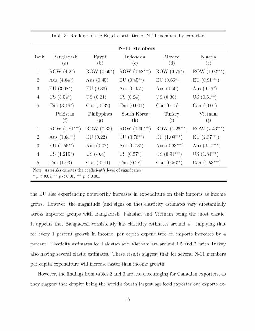
Table 3: Ranking of the Engel elasticities of N-11 members by exporters

N-11 Members

Rank Bangladesh Egypt Indonesia Mexico Nigeria(a) (b) (c) (d) (e)

1. ROW (4.2⇤) ROW (0.60⇤) ROW (0.68⇤⇤⇤) ROW (0.76⇤) ROW (1.02⇤⇤⇤)

2. Aus (4.04⇤) Aus (0.45) EU (0.45⇤⇤) EU (0.66⇤) EU (0.91⇤⇤⇤)

3. EU (3.98⇤) EU (0.38) Aus (0.45⇤) Aus (0.50) Aus (0.56⇤)

4. US (3.54⇤) US (0.21) US (0.24) US (0.30) US (0.51⇤⇤)

5. Can (3.46⇤) Can (-0.32) Can (0.001) Can (0.15) Can (-0.07)

Pakistan Philippines South Korea Turkey Vietnam(f) (g) (h) (i) (j)

1. ROW (1.81⇤⇤⇤) ROW (0.38) ROW (0.90⇤⇤⇤) ROW (1.26⇤⇤⇤) ROW (2.46⇤⇤⇤)

2. Aus (1.64⇤⇤) EU (0.22) EU (0.76⇤⇤) EU (1.09⇤⇤⇤) EU (2.37⇤⇤⇤)

3. EU (1.56⇤⇤) Aus (0.07) Aus (0.73⇤) Aus (0.93⇤⇤⇤) Aus (2.27⇤⇤⇤)

4. US (1.219⇤) US (-0.4) US (0.57⇤) US (0.91⇤⇤⇤) US (1.84⇤⇤⇤)

5. Can (1.03) Can (-0.41) Can (0.28) Can (0.56⇤⇤) Can (1.53⇤⇤⇤)

Note: Asterisks denotes the coe�cient’s level of significance⇤p < 0.05, ⇤⇤

p < 0.01, ⇤⇤⇤p < 0.001

the EU also experiencing noteworthy increases in expenditure on their imports as income

grows. However, the magnitude (and signs on the) elasticity estimates vary substantially

across importer groups with Bangladesh, Pakistan and Vietnam being the most elastic.

It appears that Bangladesh consistently has elasticity estimates around 4 – implying that

for every 1 percent growth in income, per capita expenditure on imports increases by 4

percent. Elasticity estimates for Pakistan and Vietnam are around 1.5 and 2, with Turkey

also having several elastic estimates. These results suggest that for several N-11 members

per capita expenditure will increase faster than income growth.

However, the findings from tables 2 and 3 are less encouraging for Canadian exporters, as

they suggest that despite being the world’s fourth largest agrifood exporter our exports ex-

17

perience smaller increases in expenditure as BRIC and N-11 members grow, relative to other

major exporters. In both tables Canada always has the lowest estimated Engel elasticities.

Despite confronting relative weaker demand, the silver lining is that Canadian exporters still

have hopeful prospects, as the three aforementioned N-11 members (Bangladesh, Pakistan,

and Vietnam) have Engel elasticities in excess of one, suggesting that per capita expendi-

ture on agrifood imports will increase more than proportionally with income growth. Two

members of the BRICs (India and China) also deserve a closer look. Despite demonstrating

slightly lower Engel elasticities relative to the previously mentioned N-11 members, their

sheer population sizes (of 1.22 and 1.34 billion, respectively, in 2010) suggests that on the

national level their markets may still represent important sources of new import demand for

Canada, even if growth in expenditure on Canada’s exports is increasing slower than income.

Forecasts

Even if an importer has a large Engel elasticity, increases in expenditure may not result if

income and population growth do not occur. This section uses the estimated Engel elasticities

from table 6 and IMF world economic outlook projections for population and GDP per capita

to forecast the potential value of agrifood imports in 2017 (in 2010 dollars). It then contrasts

the estimated import value for the three importer groups (BRICs, N-11 and G7) with the

2010 value in order to approximate where the largest growth in expenditure will occur for

each of the exporter groups. Here we exclude forecasts for the ROW exporter group, because

of the heterogeneous composition of the group.

The forecasts were obtained by calculating the percent growth in population and real

GDP per capita (base year 2010) for each member of the N-11, G7 and BRIC to 2017.16 It is

16We include forecasts for the G7 in order to continue the commentary on Wilson and Purushothaman(2003) and Wilson and Stupnytska (2007) projections which began in the introduction contrasting theprojected economic growth of the N-11 and BRICs relative to the G7.

18

Figure 3: Value of Agrifood Imports, 2010 and 2017

assumed that expenditure on agrifood products is homogenous of degree one in population

growth (which is inherent in the model), implying that a one percent increase in population

translates to a one percent increase in expenditure. Since the Engel elasticities represent the

e↵ect of a one percent increase in GDP per capita, the respective estimated parameters from

table 6 were multiplied by the percentage growth in real GDP per capita in order to obtain

the percentage increase in the value of agrifood imports attributable to income growth. The

percent increase (or decrease) in the value of agrifood imports between 2010 and 2017 for

each member of the importing groups (i.e. the G7, the BRICs or the N-11) was then obtained

by adding the percent increase in expenditure attributable to income and population growth

and multiplying it by the 2010 value of agrifood imports from each of the four major exporter

groups (Canada, Australia, EU-27 and the U.S.) (United Nations, 2010). The cumulative

growth in value for each importing group was then obtained by summing the increases in

the value of agrifood imports of each member, for each exporter.

As shown in figure 3, for all four exporters the G7 represents the largest importer in both

19

2010 and 2017 (in terms of value). However, Australia has the smallest values for this group

of roughly $7.92 billion in 2010 and $9.65 billion in 2017, this is likely attributable to the

fact that the United States, Canada and several of the largest members of the EU (France,

Germany, Italy and the United Kingdom) make up the majority of the G7. In contrast,

the EU-27 appears to have the largest gains in absolute terms as the value of their agrifood

imports increase $40.94 billion, again, this is likely due to the fact that four of the seven

members of the G7 are members of the EU.

The United States has the largest value of exports to the BRICs ($33.9 billion) and N-11

($36.1 billion) in 2017. While the estimated Engel elasticities faced by the US are not the

largest, and income growth is constant for each importer across the various exporters, they

experience larger increases due to the fact that their 2010 value of agrifood imports are the

largest for the latter two groups.

In terms of absolute value, in figure 3 it appears that Canada faces the lowest prospects

in 2017, with the exception of Australian exports to the G7. However, the absolute value of

agrifood imports only tells one part of the story, if Canada is to achieve the stated objective

of increasing the value of agrifood exports, the relative gain in the value of exports is of

greater strategic importance – i.e. where are the largest percentage increases going to occur

for each exporter. Figure 4 illustrates this.

In relative terms, it appears that the BRIC nations followed by the N-11 represent the

largest regions of increase for all four exporters. This supports Wilson and Purushothaman

(2003) hypothesis that rising incomes could translate into increased demand for a variety

of commodities. Australia, the US and the EU all see the value of their exports to the

BRICs increase by 80-100 percent, while the increases are more tempered for Canada at 60

percent of the 2010 value. This exercise reveals that Australia and the EU experience the

largest relative increases in the value of agrifood exports to the N-11 of 70 and 65 percent,

respectively. Percent gains in the value of exports to the G7 appear to be relatively similar

20

Figure 4: Percent increase in the value of agrifood imports, 2010-2017

across exporters and more moderate relative to the other two importer groups.

The focus of this study is not only on the potential gains from income and population

growth in the N-11 and BRICs relative to other major exporters, but also the gains for

Canada. In terms of percentage increases of the value of imports from 2010 to 2017, the

largest are for Bangladesh (135.9 percent) and Vietnam (135.9 percent), followed by China

(72.3 percent), Pakistan (63.5 percent), India (59.5 percent) and Turkey (41 percent). How-

ever, as figure 5 shows, in absolute terms the largest gain in value between 2000-2017 occurs

from trade with China (roughly $ 2.03 billion), with Bangladesh ($681.8 million), India

($327.39 million), Mexico ($210.2 million), and Pakistan ($208.6) also representing substan-

tial gains. In short, the forecasting exercise suggests that if the IMF forecasts for population

and income (GDP per capita) growth to 2017 are accurate, and holding prices constant, then

the cumulative value of Canadian agrifood exports to the BRICs and N-11 could roughly

total $11.17 billion (in 2010 dollars) – a $3.65 billion dollar increase from the 2010 total.

21

Figure 5: Increased in Value of Canadian agrifood imports by importer (2010-2017)

Conclusions

This study attempted to assess whether income growth in the Next-11 and BRICs has

translated into increased expenditure on Canadian agrifood imports. In short, the answer is

mixed. While Engel elasticity estimates are large for several BRIC (India and China) and N-

11 members (Bangladesh, Pakistan, and Vietnam) across all exporter groups, income growth

appears to have a relatively smaller impact on expenditure on Canadian agrifood exports

relative to other major exporters. For several members of the aforementioned groups, income

appears to have no, or even a negative e↵ect on per capita expenditure for Canadian exports.

This is not always the case for other exporters. However, despite this relative disadvantage,

trade is not a zero sum game. Estimates for Bangladesh, Pakistan and Vietnam indicate

that expenditure may increase at a disproportionately larger rate relative to income growth

for agrifood importers from all major exporters included in the sample. Thus, the results

suggest that Canada can experience potential gains from engaging in trade with the latter

22

countries.

A forecasting exercise revealed that the G7 still represents larger markets in terms of the

absolute value of imports, but the BRICs and N-11 have the largest percentage increases

for all exporters. This finding loosely coincides with Wilson and Purushothaman (2003)

and Wilson and Stupnytska (2007) predictions, as their projections continue to 2050, while

ours are more moderate extending to 2017, suggesting that the value of agrifood imports by

these two groups could continue to grow. Nevertheless from a Canadian perspective, relative

to the other exporter groups, Canada is projected to gain the least from income growth

in the BRICs and N-11 when compared to the exporter groups analyzed. However, this

does not preclude Canada from experiencing notable gains from economic growth within the

group. If the IMF’s income and population projections materialize in 2017, Canada could

see substantial increases in the absolute value of imports (from their 2010 values) in China

($2.03 billion), Bangladesh ($681.8 million), India ($327.4 million), Mexico ($210.2 million),

and Pakistan ($208.6 million). Thus, despite the tempered gains relative to other major

exporters, Canada still seeks to benefit.

We estimated the Engel elasticities faced by five exporters for five importer groups, but

the analysis is limited in that it does not explain what influences the variation in the Engel

elasticities across exporters – i.e. why does Canada face lower Engel elasticities? Based

on the findings of Haq and Meilke (2009b), we speculate that it may have something to do

with export composition and consumer preferences in the importing countries. This is worth

while a question for future research.

23

Table 4: Specification 1

Heckman Marginal E↵ects SubsampleCoe�cients Conditional Unconditional OLS

Aus-LI 0.656⇤⇤⇤ 0.653⇤⇤⇤ 0.656⇤⇤⇤ 0.655⇤⇤⇤

(0.124) (0.123) (0.124) (0.124)

Aus-MI 0.485⇤⇤⇤ 0.482⇤⇤⇤ 0.485⇤⇤⇤ 0.483⇤⇤⇤

(0.0838) (0.0834) (0.0838) (0.0840)

Aus-HI 0.627⇤⇤⇤ 0.624⇤⇤⇤ 0.627⇤⇤⇤ 0.626⇤⇤⇤

(0.0719) (0.0716) (0.0719) (0.0720)

Aus-N11 0.563⇤⇤⇤ 0.561⇤⇤⇤ 0.563⇤⇤⇤ 0.562⇤⇤⇤

(0.109) (0.109) (0.109) (0.110)

Aus-BRIC 0.376⇤⇤⇤ 0.375⇤⇤⇤ 0.376⇤⇤⇤ 0.373⇤⇤⇤

(0.0948) (0.0944) (0.0948) (0.0950)

ROW-LI 1.013⇤⇤⇤ 1.009⇤⇤⇤ 1.013⇤⇤⇤ 1.012⇤⇤⇤

(0.0601) (0.0599) (0.0601) (0.0602)

ROW-MI 0.950⇤⇤⇤ 0.946⇤⇤⇤ 0.950⇤⇤⇤ 0.949⇤⇤⇤

(0.0505) (0.0503) (0.0505) (0.0506)

ROW-HI 0.961⇤⇤⇤ 0.957⇤⇤⇤ 0.961⇤⇤⇤ 0.960⇤⇤⇤

(0.0485) (0.0483) (0.0485) (0.0486)

ROW-N11 0.841⇤⇤⇤ 0.837⇤⇤⇤ 0.841⇤⇤⇤ 0.840⇤⇤⇤

(0.0856) (0.0852) (0.0856) (0.0857)

ROW-BRIC 0.876⇤⇤⇤ 0.872⇤⇤⇤ 0.876⇤⇤⇤ 0.873⇤⇤⇤

(0.0648) (0.0645) (0.0648) (0.0649)

Can-LI 0.592⇤⇤⇤ 0.590⇤⇤⇤ 0.592⇤⇤⇤ 0.591⇤⇤⇤

(0.0884) (0.0881) (0.0884) (0.0886)

Can-MI 0.494⇤⇤⇤ 0.492⇤⇤⇤ 0.494⇤⇤⇤ 0.492⇤⇤⇤

(0.0701) (0.0699) (0.0701) (0.0703)

Can-HI 0.488⇤⇤⇤ 0.486⇤⇤⇤ 0.488⇤⇤⇤ 0.487⇤⇤⇤

(0.0632) (0.0629) (0.0632) (0.0633)

Can-N11 0.399⇤⇤⇤ 0.397⇤⇤⇤ 0.399⇤⇤⇤ 0.397⇤⇤⇤

(0.0984) (0.0980) (0.0984) (0.0986)

Can-BRIC 0.370⇤⇤⇤ 0.368⇤⇤⇤ 0.370⇤⇤⇤ 0.367⇤⇤⇤

(0.0837) (0.0834) (0.0837) (0.0839)

US-LI 0.749⇤⇤⇤ 0.746⇤⇤⇤ 0.749⇤⇤⇤ 0.748⇤⇤⇤

(0.0742) (0.0739) (0.0742) (0.0744)

US-MI 0.712⇤⇤⇤ 0.709⇤⇤⇤ 0.712⇤⇤⇤ 0.710⇤⇤⇤

(0.0604) (0.0601) (0.0604) (0.0605)

US-HI 0.693⇤⇤⇤ 0.690⇤⇤⇤ 0.693⇤⇤⇤ 0.692⇤⇤⇤

(0.0552) (0.0550) (0.0552) (0.0553)

US-N11 0.638⇤⇤⇤ 0.635⇤⇤⇤ 0.638⇤⇤⇤ 0.637⇤⇤⇤

(0.0939) (0.0936) (0.0939) (0.0941)

24

Table 4 – continued from previous page

Heckman Marginal E↵ects SubsampleConditional Unconditional OLS

US-BRIC 0.578⇤⇤⇤ 0.575⇤⇤⇤ 0.578⇤⇤⇤ 0.575⇤⇤⇤

(0.0769) (0.0765) (0.0769) (0.0770)

EU-LI 1.095⇤⇤⇤ 1.090⇤⇤⇤ 1.095⇤⇤⇤ 1.096⇤⇤⇤

(0.0549) (0.0547) (0.0549) (0.0551)

EU-MI 1.022⇤⇤⇤ 1.018⇤⇤⇤ 1.022⇤⇤⇤ 1.023⇤⇤⇤

(0.0485) (0.0483) (0.0485) (0.0486)

EU-HI 0.995⇤⇤⇤ 0.991⇤⇤⇤ 0.995⇤⇤⇤ 0.996⇤⇤⇤

(0.0470) (0.0468) (0.0470) (0.0471)

EU-BRIC 0.839⇤⇤⇤ 0.836⇤⇤⇤ 0.839⇤⇤⇤ 0.839⇤⇤⇤

(0.0637) (0.0635) (0.0637) (0.0639)

EU-N11 0.850⇤⇤⇤ 0.846⇤⇤⇤ 0.850⇤⇤⇤ 0.851⇤⇤⇤

(0.0840) (0.0837) (0.0840) (0.0842)

Adjacent 0.224⇤⇤⇤ 0.277⇤⇤⇤ 0.224⇤⇤⇤ 0.221⇤⇤⇤

(0.0412) (0.0492) (0.0415) (0.0413)

Common 0.494⇤⇤⇤ 0.541⇤⇤⇤ 0.494⇤⇤⇤ 0.495⇤⇤⇤

Language (0.0301) (0.0320) (0.0301) (0.0302)

Colony 0.558⇤⇤⇤ 0.537⇤⇤⇤ 0.558⇤⇤⇤ 0.559⇤⇤⇤

(0.0392) (0.0430) (0.0393) (0.0393)

lnDistance -1.408⇤⇤⇤ -1.454⇤⇤⇤ -1.408⇤⇤⇤ -1.410⇤⇤⇤

(0.0135) (0.0158) (0.0142) (0.0136)

PTA 0.113⇤⇤⇤ 0.180⇤⇤⇤ 0.114⇤⇤⇤ 0.111⇤⇤⇤

(0.0237) (0.0257) (0.0239) (0.0238)

athrho -0.0366⇤⇤⇤

(⇢) (0.00876)

lnsigma 0.328⇤⇤⇤

(ln�) (0.00644)

Adjusted R

2 0.990Log-likelihood -78926.3 -70790.1

F-test 50769.2Chi2 7904112.5

Observations 47360 47360 47360 40513Marginal e↵ects; Standard errors in parentheses⇤p < 0.05, ⇤⇤

p < 0.01, ⇤⇤⇤p < 0.001

25

Tab

le5:

Waldtestsforequalityof

Engelelasticities

facedby

exporters

Exp

orterElasticities

Joint

Australia

ROW

US

EU-27

Equ

ality

(a)

(b)

(c)

(d)

(e)

Low

Income

0.237

29.63⇤

⇤⇤3.129⇤

45.60⇤

⇤⇤79.72⇤

⇤⇤

(0.627)

(0.00)

(0.077)

(0.00)

(0.00)

Middle

Income

0.0146

71.35⇤

⇤⇤11.88

⇤⇤⇤

100.7⇤

⇤⇤186.7⇤

⇤⇤

(0.904)

(0.00)

(0.001)

(0.00)

(0.00)

Can

adian

HighIncome

4.219⇤

⇤111.7⇤

⇤⇤15.37⇤

⇤⇤134.6⇤

⇤⇤228.7⇤

⇤⇤

Elasticities

(0.04)

(0.00)

(0.00)

(0.00)

(0.00)

BRIC

s0.00496

68.94⇤

⇤⇤8.174⇤

⇤⇤30.35⇤

⇤⇤132.9⇤

⇤⇤

(0.944)

(0.00)

(0.004)

(0.00)

(0.00)

N-11

3.496⇤

62.91⇤

⇤⇤12.14⇤

⇤⇤69.00⇤

⇤⇤96.45⇤

⇤⇤

(0.062)

(0.00)

(0.00)

(0.00)

(0.00)

Marginal

e↵ects;Standarderrors

inparentheses

⇤p<

0.05,⇤⇤

p<

0.01,⇤⇤

⇤p<

0.001

26

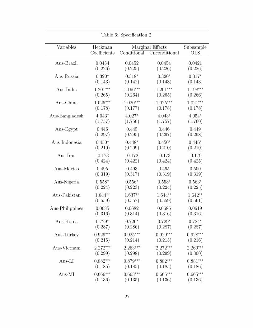
Table 6: Specification 2

Variables Heckman Marginal E↵ects SubsampleCoe�cients Conditional Unconditional OLS

Aus-Brazil 0.0454 0.0452 0.0454 0.0421(0.226) (0.225) (0.226) (0.226)

Aus-Russia 0.320⇤ 0.318⇤ 0.320⇤ 0.317⇤

(0.143) (0.142) (0.143) (0.143)

Aus-India 1.201⇤⇤⇤ 1.196⇤⇤⇤ 1.201⇤⇤⇤ 1.198⇤⇤⇤

(0.265) (0.264) (0.265) (0.266)

Aus-China 1.025⇤⇤⇤ 1.020⇤⇤⇤ 1.025⇤⇤⇤ 1.021⇤⇤⇤

(0.178) (0.177) (0.178) (0.178)

Aus-Bangladesh 4.043⇤ 4.027⇤ 4.043⇤ 4.054⇤

(1.757) (1.750) (1.757) (1.760)

Aus-Egypt 0.446 0.445 0.446 0.449(0.297) (0.295) (0.297) (0.298)

Aus-Indonesia 0.450⇤ 0.448⇤ 0.450⇤ 0.446⇤

(0.210) (0.209) (0.210) (0.210)

Aus-Iran -0.173 -0.172 -0.173 -0.179(0.424) (0.422) (0.424) (0.425)

Aus-Mexico 0.495 0.493 0.495 0.500(0.319) (0.317) (0.319) (0.319)

Aus-Nigeria 0.558⇤ 0.556⇤ 0.558⇤ 0.563⇤

(0.224) (0.223) (0.224) (0.225)

Aus-Pakistan 1.644⇤⇤ 1.637⇤⇤ 1.644⇤⇤ 1.642⇤⇤

(0.559) (0.557) (0.559) (0.561)

Aus-Philippines 0.0685 0.0682 0.0685 0.0619(0.316) (0.314) (0.316) (0.316)

Aus-Korea 0.729⇤ 0.726⇤ 0.729⇤ 0.724⇤

(0.287) (0.286) (0.287) (0.287)

Aus-Turkey 0.929⇤⇤⇤ 0.925⇤⇤⇤ 0.929⇤⇤⇤ 0.928⇤⇤⇤

(0.215) (0.214) (0.215) (0.216)

Aus-Vietnam 2.272⇤⇤⇤ 2.263⇤⇤⇤ 2.272⇤⇤⇤ 2.269⇤⇤⇤

(0.299) (0.298) (0.299) (0.300)

Aus-LI 0.882⇤⇤⇤ 0.879⇤⇤⇤ 0.882⇤⇤⇤ 0.881⇤⇤⇤

(0.185) (0.185) (0.185) (0.186)

Aus-MI 0.666⇤⇤⇤ 0.663⇤⇤⇤ 0.666⇤⇤⇤ 0.665⇤⇤⇤

(0.136) (0.135) (0.136) (0.136)

27


Variables Heckman Marginal E↵ects SubsampleConditional Unconditional OLS

Aus-HI 0.779⇤⇤⇤ 0.776⇤⇤⇤ 0.779⇤⇤⇤ 0.778⇤⇤⇤

(0.112) (0.112) (0.112) (0.113)

Can-Brazil -0.154 -0.154 -0.154 -0.158(0.204) (0.203) (0.204) (0.205)

Can-Russia -0.0891 -0.0887 -0.0891 -0.0921(0.107) (0.106) (0.107) (0.107)

Can-India 0.757⇤⇤ 0.754⇤⇤ 0.757⇤⇤ 0.754⇤⇤

(0.238) (0.237) (0.238) (0.239)

Can-China 0.642⇤⇤⇤ 0.639⇤⇤⇤ 0.642⇤⇤⇤ 0.637⇤⇤⇤

(0.140) (0.140) (0.140) (0.141)

Can-Bangladesh 3.458⇤ 3.444⇤ 3.458⇤ 3.468⇤

(1.752) (1.745) (1.752) (1.755)

Can-Egypt -0.321 -0.320 -0.321 -0.319(0.278) (0.277) (0.278) (0.279)

Can-Indonesia 0.000740 0.000737 0.000740 -0.00268(0.179) (0.178) (0.179) (0.179)

Can-Iran -0.688 -0.685 -0.688 -0.694(0.409) (0.408) (0.409) (0.410)

Can-Mexico 0.145 0.144 0.145 0.149(0.306) (0.304) (0.306) (0.306)

Can-Nigeria -0.0683 -0.0681 -0.0683 -0.0643(0.189) (0.189) (0.189) (0.190)

Can-Pakistan 1.034 1.030 1.034 1.031(0.547) (0.545) (0.547) (0.549)

Can-Philippines -0.407 -0.406 -0.407 -0.414(0.295) (0.293) (0.295) (0.295)

Can-Korea 0.275 0.274 0.275 0.270(0.274) (0.273) (0.274) (0.275)

Can-Turkey 0.560⇤⇤ 0.557⇤⇤ 0.560⇤⇤ 0.558⇤⇤

(0.192) (0.191) (0.192) (0.193)

Can-Vietnam 1.530⇤⇤⇤ 1.524⇤⇤⇤ 1.530⇤⇤⇤ 1.526⇤⇤⇤

(0.273) (0.272) (0.273) (0.273)

Can-LI 0.411⇤⇤⇤ 0.409⇤⇤⇤ 0.411⇤⇤⇤ 0.410⇤⇤⇤

(0.116) (0.116) (0.116) (0.117)

28



Can-MI 0.362⇤⇤⇤ 0.360⇤⇤⇤ 0.362⇤⇤⇤ 0.360⇤⇤⇤

(0.0912) (0.0909) (0.0912) (0.0916)

Can-HI 0.386⇤⇤⇤ 0.384⇤⇤⇤ 0.386⇤⇤⇤ 0.384⇤⇤⇤

(0.0799) (0.0796) (0.0799) (0.0802)

EU-Brazil 0.469⇤ 0.467⇤ 0.469⇤ 0.467⇤

(0.194) (0.193) (0.194) (0.194)

EU-Russia 0.688⇤⇤⇤ 0.686⇤⇤⇤ 0.688⇤⇤⇤ 0.688⇤⇤⇤

(0.0692) (0.0689) (0.0692) (0.0694)

EU-India 1.192⇤⇤⇤ 1.187⇤⇤⇤ 1.192⇤⇤⇤ 1.192⇤⇤⇤

(0.212) (0.212) (0.212) (0.213)

EU-China 1.049⇤⇤⇤ 1.044⇤⇤⇤ 1.049⇤⇤⇤ 1.047⇤⇤⇤

(0.110) (0.109) (0.110) (0.110)

EU-Bangladesh 3.975⇤ 3.959⇤ 3.975⇤ 3.986⇤

(1.750) (1.743) (1.750) (1.752)

EU-Egypt 0.376 0.375 0.376 0.381(0.263) (0.262) (0.263) (0.264)

EU-Indonesia 0.452⇤⇤ 0.450⇤⇤ 0.452⇤⇤ 0.451⇤⇤

(0.157) (0.156) (0.157) (0.157)

EU-Iran -0.324 -0.322 -0.324 -0.329(0.399) (0.397) (0.399) (0.400)

EU-Mexico 0.659⇤ 0.656⇤ 0.659⇤ 0.666⇤

(0.299) (0.298) (0.299) (0.300)

EU-Nigeria 0.907⇤⇤⇤ 0.903⇤⇤⇤ 0.907⇤⇤⇤ 0.912⇤⇤⇤

(0.159) (0.159) (0.159) (0.160)

EU-Pakistan 1.557⇤⇤ 1.550⇤⇤ 1.557⇤⇤ 1.556⇤⇤

(0.541) (0.539) (0.541) (0.542)

EU-Philippines 0.220 0.219 0.220 0.216(0.283) (0.282) (0.283) (0.284)

EU-Korea 0.763⇤⇤ 0.760⇤⇤ 0.763⇤⇤ 0.760⇤⇤

(0.267) (0.266) (0.267) (0.268)

EU-Turkey 1.090⇤⇤⇤ 1.086⇤⇤⇤ 1.090⇤⇤⇤ 1.092⇤⇤⇤

(0.177) (0.176) (0.177) (0.177)

EU-Vietnam 2.371⇤⇤⇤ 2.361⇤⇤⇤ 2.371⇤⇤⇤ 2.369⇤⇤⇤

(0.252) (0.251) (0.252) (0.253)

EU-LI 1.054⇤⇤⇤ 1.049⇤⇤⇤ 1.054⇤⇤⇤ 1.054⇤⇤⇤

29



(0.0562) (0.0560) (0.0562) (0.0564)

EU-MI 0.997⇤⇤⇤ 0.992⇤⇤⇤ 0.997⇤⇤⇤ 0.997⇤⇤⇤

(0.0492) (0.0490) (0.0492) (0.0494)

EU-HI 0.978⇤⇤⇤ 0.974⇤⇤⇤ 0.978⇤⇤⇤ 0.979⇤⇤⇤

(0.0475) (0.0473) (0.0475) (0.0476)

US-Brazil 0.000333 0.000332 0.000333 -0.00336(0.198) (0.197) (0.198) (0.198)

US-Russia 0.236⇤⇤ 0.235⇤⇤ 0.236⇤⇤ 0.233⇤⇤

(0.0885) (0.0881) (0.0885) (0.0888)

US-India 0.906⇤⇤⇤ 0.902⇤⇤⇤ 0.906⇤⇤⇤ 0.903⇤⇤⇤

(0.226) (0.225) (0.226) (0.227)

US-China 0.892⇤⇤⇤ 0.888⇤⇤⇤ 0.892⇤⇤⇤ 0.888⇤⇤⇤

(0.128) (0.127) (0.128) (0.128)

US-Bangladesh 3.543⇤ 3.529⇤ 3.543⇤ 3.553⇤

(1.750) (1.743) (1.750) (1.752)

US-Egypt 0.213 0.212 0.213 0.216(0.270) (0.269) (0.270) (0.271)

US-Indonesia 0.236 0.235 0.236 0.233(0.168) (0.167) (0.168) (0.169)

US-Iran -1.157⇤⇤ -1.152⇤⇤ -1.157⇤⇤ -1.163⇤⇤

(0.412) (0.411) (0.412) (0.413)

US-Mexico 0.302 0.301 0.302 0.307(0.302) (0.300) (0.302) (0.302)

US-Nigeria 0.505⇤⇤ 0.503⇤⇤ 0.505⇤⇤ 0.509⇤⇤

(0.176) (0.175) (0.176) (0.177)

US-Pakistan 1.219⇤ 1.214⇤ 1.219⇤ 1.217⇤

(0.542) (0.540) (0.542) (0.544)

US-Philippines -0.138 -0.138 -0.138 -0.145(0.288) (0.287) (0.288) (0.289)

US-Korea 0.571⇤ 0.569⇤ 0.571⇤ 0.566⇤

(0.271) (0.269) (0.271) (0.271)

US-Turkey 0.907⇤⇤⇤ 0.903⇤⇤⇤ 0.907⇤⇤⇤ 0.906⇤⇤⇤

(0.184) (0.183) (0.184) (0.185)

US-Vietnam 1.841⇤⇤⇤ 1.833⇤⇤⇤ 1.841⇤⇤⇤ 1.837⇤⇤⇤

(0.263) (0.262) (0.263) (0.263)

30



US-LI 0.587⇤⇤⇤ 0.584⇤⇤⇤ 0.587⇤⇤⇤ 0.585⇤⇤⇤

(0.0929) (0.0926) (0.0929) (0.0932)

US-MI 0.594⇤⇤⇤ 0.591⇤⇤⇤ 0.594⇤⇤⇤ 0.592⇤⇤⇤

(0.0733) (0.0730) (0.0733) (0.0736)

US-HI 0.601⇤⇤⇤ 0.599⇤⇤⇤ 0.601⇤⇤⇤ 0.600⇤⇤⇤

(0.0650) (0.0647) (0.0650) (0.0652)

ROW-Brazil 0.605⇤⇤ 0.602⇤⇤ 0.605⇤⇤ 0.602⇤⇤

(0.191) (0.190) (0.191) (0.192)

ROW-Russia 0.775⇤⇤⇤ 0.772⇤⇤⇤ 0.775⇤⇤⇤ 0.773⇤⇤⇤

(0.0702) (0.0699) (0.0702) (0.0704)

ROW-India 1.624⇤⇤⇤ 1.617⇤⇤⇤ 1.624⇤⇤⇤ 1.621⇤⇤⇤

(0.216) (0.216) (0.216) (0.217)

ROW-China 1.363⇤⇤⇤ 1.357⇤⇤⇤ 1.363⇤⇤⇤ 1.359⇤⇤⇤

(0.115) (0.114) (0.115) (0.115)

ROW-Bangladesh 4.196⇤ 4.179⇤ 4.196⇤ 4.207⇤

(1.750) (1.742) (1.750) (1.752)

ROW-Egypt 0.600⇤ 0.598⇤ 0.600⇤ 0.603⇤

(0.264) (0.263) (0.264) (0.265)

ROW-Indonesia 0.678⇤⇤⇤ 0.676⇤⇤⇤ 0.678⇤⇤⇤ 0.676⇤⇤⇤

(0.157) (0.156) (0.157) (0.158)

ROW-Iran -0.0992 -0.0988 -0.0992 -0.105(0.401) (0.400) (0.401) (0.402)

ROW-Mexico 0.762⇤ 0.759⇤ 0.762⇤ 0.767⇤

(0.298) (0.297) (0.298) (0.299)

ROW-Nigeria 1.024⇤⇤⇤ 1.020⇤⇤⇤ 1.024⇤⇤⇤ 1.028⇤⇤⇤

(0.156) (0.155) (0.156) (0.156)

ROW-Pakistan 1.812⇤⇤⇤ 1.804⇤⇤⇤ 1.812⇤⇤⇤ 1.810⇤⇤⇤

(0.536) (0.534) (0.536) (0.537)

ROW-Philippines 0.377 0.375 0.377 0.371(0.282) (0.281) (0.282) (0.283)

ROW-Korea 0.898⇤⇤⇤ 0.894⇤⇤⇤ 0.898⇤⇤⇤ 0.893⇤⇤⇤

(0.267) (0.266) (0.267) (0.267)

ROW-Turkey 1.258⇤⇤⇤ 1.253⇤⇤⇤ 1.258⇤⇤⇤ 1.258⇤⇤⇤

(0.176) (0.175) (0.176) (0.177)

31



ROW-Vietnam 2.461⇤⇤⇤ 2.451⇤⇤⇤ 2.461⇤⇤⇤ 2.458⇤⇤⇤

(0.251) (0.250) (0.251) (0.252)

ROW-LI 1.183⇤⇤⇤ 1.179⇤⇤⇤ 1.183⇤⇤⇤ 1.183⇤⇤⇤

(0.0638) (0.0636) (0.0638) (0.0640)

ROW-MI 1.088⇤⇤⇤ 1.084⇤⇤⇤ 1.088⇤⇤⇤ 1.087⇤⇤⇤

(0.0532) (0.0530) (0.0532) (0.0534)

ROW-HI 1.077⇤⇤⇤ 1.073⇤⇤⇤ 1.077⇤⇤⇤ 1.076⇤⇤⇤

(0.0505) (0.0503) (0.0505) (0.0507)

Adjacent 0.209⇤⇤⇤ 0.260⇤⇤⇤ 0.209⇤⇤⇤ 0.205⇤⇤⇤

(0.0417) (0.0488) (0.0419) (0.0419)

Common 0.513⇤⇤⇤ 0.559⇤⇤⇤ 0.513⇤⇤⇤ 0.513⇤⇤⇤

Language (0.0306) (0.0323) (0.0305) (0.0307)

Colony 0.540⇤⇤⇤ 0.520⇤⇤⇤ 0.539⇤⇤⇤ 0.541⇤⇤⇤

(0.0394) (0.0427) (0.0394) (0.0395)

lnDistance -1.404⇤⇤⇤ -1.449⇤⇤⇤ -1.404⇤⇤⇤ -1.406⇤⇤⇤

(0.0138) (0.0150) (0.0139) (0.0138)

PTA 0.131⇤⇤⇤ 0.196⇤⇤⇤ 0.132⇤⇤⇤ 0.129⇤⇤⇤

(0.0239) (0.0252) (0.0239) (0.0240)

athrho -0.0424⇤⇤⇤

(⇢) (0.00886)

lnsigma 0.320⇤⇤⇤

(ln�) (0.00651)

Adjusted R

2 0.990Log-Likelihood -78563.8 -70428.7

F-test 41453.2Chi2 9113480.9

Observations 47360 47360 47360 40513

Marginal e↵ects; Standard errors in parentheses⇤p < 0.05, ⇤⇤

p < 0.01, ⇤⇤⇤p < 0.001

32

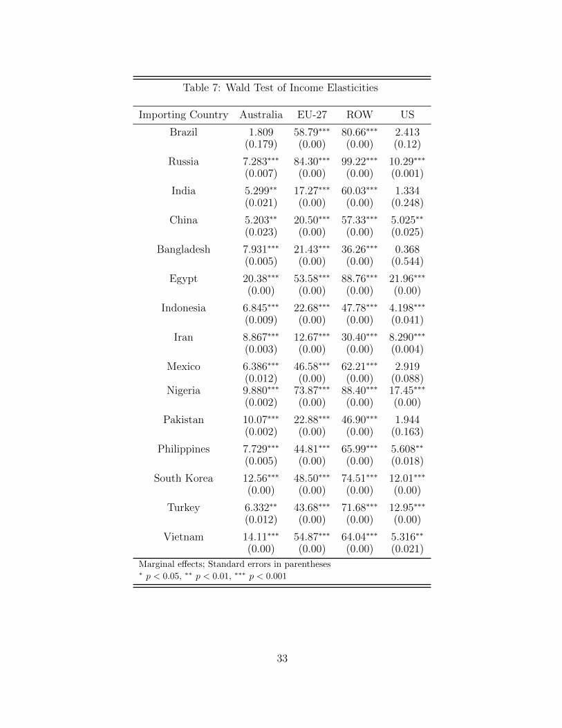
Table 7: Wald Test of Income Elasticities

Importing Country Australia EU-27 ROW US

Brazil 1.809 58.79⇤⇤⇤ 80.66⇤⇤⇤ 2.413(0.179) (0.00) (0.00) (0.12)

Russia 7.283⇤⇤⇤ 84.30⇤⇤⇤ 99.22⇤⇤⇤ 10.29⇤⇤⇤

(0.007) (0.00) (0.00) (0.001)

India 5.299⇤⇤ 17.27⇤⇤⇤ 60.03⇤⇤⇤ 1.334(0.021) (0.00) (0.00) (0.248)

China 5.203⇤⇤ 20.50⇤⇤⇤ 57.33⇤⇤⇤ 5.025⇤⇤

(0.023) (0.00) (0.00) (0.025)

Bangladesh 7.931⇤⇤⇤ 21.43⇤⇤⇤ 36.26⇤⇤⇤ 0.368(0.005) (0.00) (0.00) (0.544)

Egypt 20.38⇤⇤⇤ 53.58⇤⇤⇤ 88.76⇤⇤⇤ 21.96⇤⇤⇤

(0.00) (0.00) (0.00) (0.00)

Indonesia 6.845⇤⇤⇤ 22.68⇤⇤⇤ 47.78⇤⇤⇤ 4.198⇤⇤⇤

(0.009) (0.00) (0.00) (0.041)

Iran 8.867⇤⇤⇤ 12.67⇤⇤⇤ 30.40⇤⇤⇤ 8.290⇤⇤⇤

(0.003) (0.00) (0.00) (0.004)

Mexico 6.386⇤⇤⇤ 46.58⇤⇤⇤ 62.21⇤⇤⇤ 2.919(0.012) (0.00) (0.00) (0.088)

Nigeria 9.880⇤⇤⇤ 73.87⇤⇤⇤ 88.40⇤⇤⇤ 17.45⇤⇤⇤

(0.002) (0.00) (0.00) (0.00)

Pakistan 10.07⇤⇤⇤ 22.88⇤⇤⇤ 46.90⇤⇤⇤ 1.944(0.002) (0.00) (0.00) (0.163)

Philippines 7.729⇤⇤⇤ 44.81⇤⇤⇤ 65.99⇤⇤⇤ 5.608⇤⇤

(0.005) (0.00) (0.00) (0.018)

South Korea 12.56⇤⇤⇤ 48.50⇤⇤⇤ 74.51⇤⇤⇤ 12.01⇤⇤⇤

(0.00) (0.00) (0.00) (0.00)

Turkey 6.332⇤⇤ 43.68⇤⇤⇤ 71.68⇤⇤⇤ 12.95⇤⇤⇤

(0.012) (0.00) (0.00) (0.00)

Vietnam 14.11⇤⇤⇤ 54.87⇤⇤⇤ 64.04⇤⇤⇤ 5.316⇤⇤

(0.00) (0.00) (0.00) (0.021)

Marginal e↵ects; Standard errors in parentheses⇤p < 0.05, ⇤⇤

p < 0.01, ⇤⇤⇤p < 0.001

33

References

Anderson, J., and E. van Wincoop. 2003. “Gravity with Gravitas: A Solution to the Border

Puzzle.” The American Economic Review 93:170.

Baier, S., and J. Bergstrand. 2007. “Do free trade agreements actually increase member’s

international trade?” Journal of International Economics 71:72–95.

Baier, S.L., and J.H. Bergstrand. 2004. “Economic determinants of free trade agreements.”

Journal of International Economics 64:29–63.

CAFTA. 2008. “Harvesting the WTO agreement.”

Cairns, A.P., and K.D. Meilke. 2012. “The Next-11 and the BRICs: Are They the Future

Markets for Agrifood Trade?” Working Paper No. 2012-03, Canadian Agricultural Trade

Policy and Competitiveness Research Network.

CAPI. 2011. “Canada’s Agrifood Destination.” Government, Canadian Agrifood Policy In-

stitute (CAPI), Feburary.

Cranfield, J., P. Preckel, J. Eales, and T. Hertel. 2002. “Estimating Consumer Demand

Across the Development Spectrum: Maximum Likelihood Estimates of the Implicit Direct

Additivity Model.” Journal of Development Economics 68:289.

Dow, W., and E. Norton. 2003. “Choosing Between and Interpreting the Heckit and Two-

part Models for Corner Solutions.” Health Services and Outcomes Research Methodology

4:5.

Egger, P. 2000. “A note on the proper econometric specification of the gravity model.”

Economic Letters 66:25–31.

34

Grant, J., and D. Lambert. 2008. “Do Regional Trade Agreements Increase Member’s Agri-

cultural Trade?” American Journal of Agricultural Economics 90:765.

Hallak, J. 2006. “Product Quality and the Direction of Trade.” Journal of International

Economics 68:238.

Haq, Z., and K. Meilke. 2009a. “Do the BRICs and Emerging Markets Di↵er in their Agrifood

Imports?” Journal of Agricultural Economics 61:1–14.

—. 2009b. “The Role of Income in Trading-Di↵erentiated Agri-Food Products: The Case of

Canada, the United States, and Selected EU Countries.” Canadian Journal of Agricultural

Economics 57:343–363.

Haq, Z., K. Meilke, and J. Cranfield. 2010. “Does the Gravity Model Su↵er from Selection

Bias?” Working Paper No. 2010-01, Canadian Agricultural Trade Policy and Competi-

tiveness Research Network.

Head, K., and T. Mayer. 2002. “Illusory Border E↵ects: Distance Mismeasurements Inflates

Estimates of Home Bias in Trade.” CEPII Working Paper No. 2002-01, CEPII.

Heckman, J.J. 1976. “Common Structure of Statistical Models of Truncation, Sample Selec-

tion and Limited Dependent Variables and a Simple Estimator for Such Models.” Annals

of Economic and Statistical Measurement 5:475–492.

Leung, S., and S. Yu. 1996. “On Choice Between Sample Selection and Two-Part Models.”

Journal of Econometrics 72:197.

Matyas, L. 1997. “Proper Econometric Specification of the Gravity Model.” The World

Economy 20:363–368.

Mayer, T., and S. Zignago. 2005. “Market Access in Global and Regional Trade.” Cepii

working paper 2, CEPII, Feburary.

35

Puhani, P. 2000. “The Heckman Correction for Sample Selection and its Critique.” Journal

of Economic Surveys 14:53–68.

United Nations. 2010. “United Nations Commodity Trade Statistics Database.”

Wilson, D., and R. Purushothaman. 2003. “Dreaming With BRICs: The Path to 2050.”

Global economics paper no:99, Goldman Sachs.

Wilson, D., and A. Stupnytska. 2007. “The N-11: More Than an Acronym.” Global eco-

nomics paper no: 153, Goldman Sachs.

Wooldridge, J.M. 2002. Econometric Analysis of Cross Section and Panel Data. MIT Press.

WTO. 2009. “Chapter 2: Merchandise Trade by Product.” International trade statistics,

World Trade Organization.

36

canadian agrifood export performance and the growth potential...

Documents