LBNL-1006282

Can We Practically Bring Physics-

based Modeling Into Operational

Analytics Tools?

Jessica Granderson, Marco Bonvini1, Mary Ann Piette,

Janie Page, Guanjing Lin, R. Lily Hu2

1Wisker Labs

2UC Berkeley

Energy Technologies Area

August, 2016

Published in the Proceedings of the 2016 ACEEE

Summer Study on Energy Efficiency in Buildings,

Pacific Grove, CA, August 2016.

Disclaimer This document was prepared as an account of work sponsored by the United States

Government. While this document is believed to contain correct information, neither the

United States Government nor any agency thereof, nor The Regents of the University of

California, nor any of their employees, makes any warranty, express or implied, or

assumes any legal responsibility for the accuracy, completeness, or usefulness of any

information, apparatus, product, or process disclosed, or represents that its use would not

infringe privately owned rights. Reference herein to any specific commercial product,

process, or service by its trade name, trademark, manufacturer, or otherwise, does not

necessarily constitute or imply its endorsement, recommendation, or favoring by the

United States Government or any agency thereof, or The Regents of the University of

California. The views and opinions of authors expressed herein do not necessarily state or

reflect those of the United States Government or any agency thereof or The Regents of the

University of California.

Can We Practically Bring Physics-based Modeling Into Operational Analytics

Tools?

Jessica Granderson, Lawrence Berkeley National Laboratory

Marco Bonvini, Whisker Labs

Mary Ann Piette, Lawrence Berkeley National Laboratory

Janie Page, Lawrence Berkeley National Laboratory

Guanjing Lin, Lawrence Berkeley National Laboratory R.

Lily Hu, UC Berkeley

ABSTRACT

Analytics software is increasingly used to improve and maintain operational efficiency in

commercial buildings. Energy managers, owners, and operators are using a diversity of

commercial offerings often referred to as Energy Information Systems, Fault Detection and

Diagnostic (FDD) systems, or more broadly Energy Management and Information Systems, to

cost-effectively enable savings on the order of ten to twenty percent. Most of these systems use

data from meters and sensors, with rule-based and/or data-driven models to characterize system

and building behavior. In contrast, physics-based modeling uses first-principles and engineering

models (e.g., efficiency curves) to characterize system and building behavior. Historically, these

physics-based approaches have been used in the design phase of the building life cycle or in

retrofit analyses. Researchers have begun exploring the benefits of integrating physics-based

models with operational data analytics tools, bridging the gap between design and operations. In

this paper, we detail the development and operator use of a software tool that uses hybrid data-

driven and physics-based approaches to cooling plant FDD and optimization. Specifically, we

describe the system architecture, models, and FDD and optimization algorithms; advantages and

disadvantages with respect to purely data-driven approaches; and practical implications for

scaling and replicating these techniques. We conclude with an evaluation of the future potential

for such tools and future research opportunities.

Introduction

This paper presents the development of a hybrid data-driven and physics model-based

operational tool for energy efficiency in central cooling plants. The tool, PlantInsight, offers fault

detection and diagnostics (FDD) functionality, setpoint optimization, and visualization of key

performance parameters. Operational tools that combine analysis of historical data with a

representation of the physics of the building and its systems may offer increased diagnostic

power. Whereas empirical data-driven analytics permit assessment of operations based on actual

prior system performance, physics-based approaches also enable assessment relative to design

intent, and underlying physical principles. While the potential advantages of these hybrid tools

are clear, it is less clear whether they can practically be developed and deployed for routine use

in today’s buildings. In this work, we detail the development of PlantInsight, including its

architecture, model creation and calibration, and analysis algorithms. We describe development

challenges that were encountered, as well as operator reception of the tool, and savings

opportunities identified. Based on this experience we provide discussion of practical implications

for scaling and replicating these techniques, and conclude with an evaluation of the future

potential for such tools and future research opportunities. Current State of the Art

Data-driven and rule-based analytics tools, as defined in Katipamula 2005, are

increasingly used for operational efficiency in today’s commercial buildings. Energy

Management and Information Systems (EMIS) span a family of technologies and including

energy information systems (EIS), building automation systems, fault detection and diagnostics,

and monthly energy analysis tools. These tools have enabled whole-building energy savings of

up to 10-20% with rapid paybacks, often under three years (Granderson 2011, 2016). Savings are

achieved through multiple strategies such as identification of operational efficiency improvement

opportunities, fault and energy anomaly detection, and inducement of behavioral change among

occupants and operations personnel. The market for commercial analytics tools has expanded

quickly over recent years, marking one of the largest market growth areas in commercial

building technologies. In contrast to data-driven approaches, physics-based modeling tools use first-principles

and engineering models (e.g., efficiency curves) to characterize system and building behavior.

Historically, these physics-based approaches have been used in the design phase of the building

life cycle or in retrofit analyses; EnergyPlus, eQuest, Sefaira, and Integrated Environmental

Solutions (IES) VE, are just a few tools that are founded on these physics-based methods. There

are also instances of simulation models used for HVAC design, such as Trane Trace. In the

commercial market, there are a modest yet growing number of tools that have begun to

incorporate physics-based models into applications that target the identification of operational

efficiency opportunities, such as simuwatt Energy Auditor and Retroficiency Building

Efficiency Intelligence. Those that do are often used to identify capital and operational measures,

but are most commonly applied at single points in time for activities such as audits,

commissioning, and portfolio opportunity assessment, as opposed to being integrated into

continuous tools for operations staff. These examples notwithstanding, the use of hybrid data-

driven and model-based approaches for operational tools that conduct continuous fault detection

and energy use optimization is largely still the domain of exploratory research. For example, a

previous attempt to use EnergyPlus physics-based models to identify whole-building level

operational energy waste was proposed by (Pang 2012). Overview of PlantInsight: A Physics-based Operational Analytics Tool

PlantInsight is a hybrid data-driven and physics model-based operational tool for energy

efficiency in central cooling plants. It provides detection and diagnosis of three types of faults –

fan cycling, chiller cycling, and poor chiller efficiency. It also provides analysis of optimal

condenser water setpoint temperatures to minimize plant energy consumption. A calibrated

Modelica model is used in the algorithms to identify poor chiller efficiency, and optimal

condenser water temperature, while the cycling faults are identified using purely data-driven

models. In addition, the tool offers visualization for operators to track key parameters such as

cooling plant load and chilled water loop temperature. Through provision of these features,

PlantInsight targets ten percent plant energy savings, given engaged users who use the tool daily,

and are able to take action on the tool’s outputs.

Development Methodology

The development of the PlantInsight tool comprised four primary elements: model

construction and calibration, creation of FDD and optimization algorithms, architecture

definition, and operator feedback. These elements are detailed in the following subsections. Model Construction and Calibration

The Modelica models that simulate the operation of the central cooling plant were

developed using a diversity of information from the cooling plant design specifications,

nameplate data, drawings, and trend-log data. Beginning with the design drawings, the plant

configuration, components, and equipment were replicated in model form. The Modelica

Buildings Library (Wetter 2014) was used to build a representation of a specific central cooling

system a large university campus. In this case, the system included 2 interconnected chilled

water plants. The first plant contains one 2500-ton York MaxETM

YD Centrifugal Liquid Chiller

and two 1250-ton York MaxETM

YK Centrifugal Liquid Chillers, with four cooling towers and

five primary pumps. The second plant contains three 2500-ton York MaxETM

YD Centrifugal

Liquid Chillers (with space available for an additional 2500 ton chiller), three cooling towers,

and four pumps. Typical off-peak operations use the first plant exclusively, while peak summer

operations use the second plant either exclusively, or in combination with the first. Once the

plant design was represented, manufacturer data including nameplate values, chiller loading

curves, and pump curves, were used to quantify key equipment and component-level

characteristics. Finally, the specific control sequences that are in use at the plant were embedded

into the model. In-person site visits were necessary to compile all of the information needed for

model creation, since not all information was readily accessible in digital form.

Once constructed, the models were calibrated to the measured historic data from the cooling plant. The first step in calibration was to filter the historic data to that representing

steady state plant operation. From the steady state data, we ensured as large as possible a range

in the variation of each variable, for maximum coverage of operational conditions. Next, the

GenOpt (Wetter 2001) optimization engine was used to search the (un-calibrated) model

parameters to minimize the difference between the model outputs and the associated measured

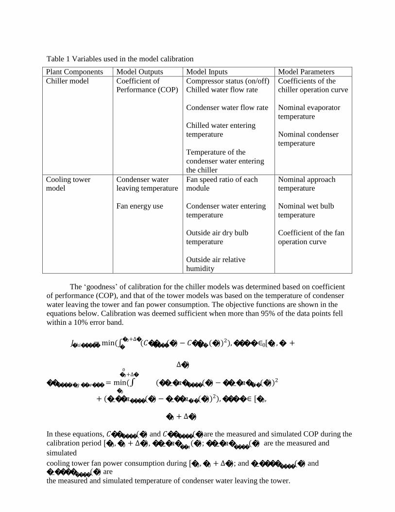
data. The variables involved in the calibration are listed in Table 1. Model parameters are values

used in the model that are known a priori, and are specific to the equipment and plant design.

�ℎ𝑖����� � ���� �𝑖� 0 0

Table 1 Variables used in the model calibration

Plant Components Model Outputs Model Inputs Model Parameters

Chiller model Coefficient of Performance (COP)

Compressor status (on/off) Chilled water flow rate

Condenser water flow rate

Chilled water entering

temperature

Temperature of the

condenser water entering

the chiller

Coefficients of the chiller operation curve

Nominal evaporator

temperature

Nominal condenser

temperature

Cooling tower model

Condenser water leaving temperature

Fan energy use

Fan speed ratio of each module

Condenser water entering

temperature

Outside air dry bulb

temperature

Outside air relative

humidity

Nominal approach temperature

Nominal wet bulb

temperature

Coefficient of the fan

operation curve

The ‘goodness’ of calibration for the chiller models was determined based on coefficient

of performance (COP), and that of the tower models was based on the temperature of condenser

water leaving the tower and fan power consumption. The objective functions are shown in the

equations below. Calibration was deemed sufficient when more than 95% of the data points fell

within a 10% error band.

𝐽 = min(∫�0 +∆�

(𝐶�� (�) − 𝐶�� (�))2 ), ��� � ∈ [� , � +

∆�) 0

�0 +∆�

������𝑖�𝑔 ��𝑤��� = min(∫ (��_�𝑎����� (�) − ��_�𝑎��𝑖� (�))2

�0

+ (�_��𝑎���� (�) − �_��𝑎�𝑖� (�))2), ��� � ∈ [�0,

�0 + ∆�)

In these equations, 𝐶������(�) and 𝐶������ (�)are the measured and simulated COP during the

calibration period [�0, �0 + ∆�), ��_�𝑎���𝑎

(�); ��_�𝑎�����

(�) are the measured and

simulated cooling tower fan power consumption during [�0, �0 + ∆�); and �_��������(�) and

�_�������� (�) are

the measured and simulated temperature of condenser water leaving the tower.

FDD and Optimization Algorithms

To-date PlantInsight addresses three faults. Poor chiller efficiency is determined by

comparing the model-predicted versus the metered coefficient of performance. Described in

detail in Bonvini 2014a, 2014b, and briefly summarized here, the FDD algorithm is based on an

advanced Bayesian nonlinear state estimation technique called Unscented Kalman Filtering

(Julier 1996) that quickly reconciles model predictions with measured data. A back smoothing

method is added to reduce the likelihood of false positives from operational variability and data

uncertainties. A clustering and decision tree analysis procedure was developed to group detected

faults based on the similarity of conditions under which they occur; similar instances are

grouped, and summarized in the tool interface to support root cause diagnostics by the operator.

First, a k-means clustering algorithm divides the observed faults into distinct operational

conditions under which the faults can be characterized. Each k cluster corresponds to a

diagnostic message for the operator (see Figure 4). Once the clusters are identified, a human

readable diagnostic message must be assigned. A decision tree is used to determine the

boundaries in the feature space that distinguish between regular and faulty data, and thus identify

them. The variables used in the decision tree, i.e. the feature space, are condenser and evaporator

water temperatures, cooling load, electric power, time of the day, outside air temperature and the

condenser and evaporator mass flow rates. The results of the decision tree are then sorted in

order of importance to find the set that best describes the majority of the faulty conditions. This

algorithm will be evaluated in field testing to assess the effectiveness of the clustering and

decision tree analysis, as well as the thresholds used in the probabilistic identification of faults.

Excessive chiller cycling and excessive cooling tower fan cycling are detected using data-

driven algorithms that rely upon chiller motor current data and fan speed data. The data is

collected every 5 minutes and interpolated to 10 seconds, using cubic interpolation (linear and

quadratic interpolation created spurious high frequencies, and large oscillations respectively).

Interpolation was needed to increase the number of data points in order to use Fourier

transformation. The time series data is transformed into the frequency domain using a Fourier

transform on a rolling two-hour window. The area under the amplitude versus frequency curve of

the Fourier transform is calculated using trapezoid integration, for the area between a frequency

of 4 cycles per hour to a frequency of 6 cycles per hour. Due to the data sampling frequency of

every 5 minutes, the shortest cycling frequency (the Nyquist frequency) that can be detected is 6

cycles per hour. Higher frequency of data collection is desirable to avoid aliasing problems but

was unfortunately not available. If the area under the curve is higher than a reference value, then

an excessive cycling fault is identified.

The optimization algorithm determines the most effective condenser water temperature

setpoint.The chillers’ efficiency increases when the temperature of condenser water entering the

chillers (Tcw,ent) decreases. On the other hand, reducing Tcw,ent may increase the energy

consumption of cooling towers. Therefore, there is an optimum condenser water temperature

setpoint for cooling towers that the total energy consumption of the chillers and the cooling

towers is minimized. To determine the optimal condenser water temperature setpoint, the

component models of multiple chillers, cooling towers and pumps were packaged into a system

model. The system model was run to predict the energy consumption under different condenser

water set points. Optimization constraints, such as the desired cooling load, were also

incorporated into the model. As with the calibration activity, GenOpt was used as the

optimization engine. The optimization period can be set to any desired value, in the case of this

work, ranging from one hour to one day. Specifically, the optimal condenser water set point is

�

𝑤� 0 0 0

�

𝑃

determined by solving the optimization problem defined in the equation below, and documented

in Huang, 2014.

min(��|�0

+Δ� 0

�0 +∆�

) = min (∫ �(����,����

(�0), �̇

�0

𝑃 (�) , � 𝑃 (�), �⃗(� ))) , for � ∈ [� , � +

∆�)

such that ����,����,𝐿 ≤ ����,���� (�0) ≤ ����,����,𝐻 ,

In these equations, ��|�0

+Δ�

0

is the total energy consumption of the chillers and cooling towers

during the optimization period [�0, �0 + ∆�), ����,���� is the condenser water set point, �̇ 𝑃 is the predicted cooling load, �𝑤� is the predicted wet bulb temperature from a weather forecast, �⃗ is the state vector of the system (e.g. equipment operating status, water temperature in chiller condenser and evaporator), and ����,����,𝐿 and ����,����,𝐻 are the low and high limits of the condenser water set point during [�0, �0 + ∆�).

Architecture

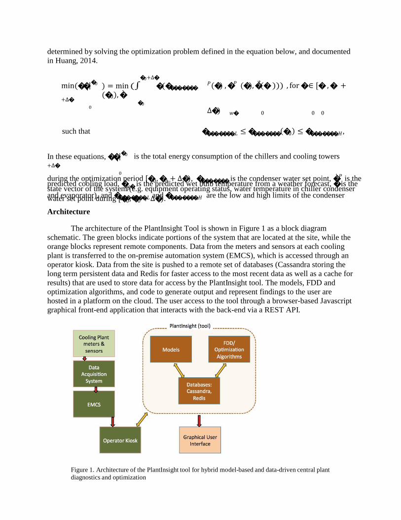
The architecture of the PlantInsight Tool is shown in Figure 1 as a block diagram

schematic. The green blocks indicate portions of the system that are located at the site, while the

orange blocks represent remote components. Data from the meters and sensors at each cooling

plant is transferred to the on-premise automation system (EMCS), which is accessed through an

operator kiosk. Data from the site is pushed to a remote set of databases (Cassandra storing the

long term persistent data and Redis for faster access to the most recent data as well as a cache for

results) that are used to store data for access by the PlantInsight tool. The models, FDD and

optimization algorithms, and code to generate output and represent findings to the user are

hosted in a platform on the cloud. The user access to the tool through a browser-based Javascript

graphical front-end application that interacts with the back-end via a REST API.

Figure 1. Architecture of the PlantInsight tool for hybrid model-based and data-driven central plant

diagnostics and optimization

Operator Feedback and Tool Reception

To ensure that the tool would be of maximum utility to plant operators, design feedback

was obtained iteratively, throughout development. The most important feedback that was (and is

being) integrated into the tool design and functionality is summarized in the following:

Add key performance indicators: Primary chilled water loop temperature, and weather

forecast are critical parameters that are tracked by the operations staff. In addition, staff

also requested that the tool-predicted plant load forecast be added to the interface. Since

these variable are tracked on a continual basis under existing operations, it was important

that they be included in the PlantInsight tool. If excluded the tool would be less likely to

be integrated into daily management processes because it would lack the most valuable

monitoring features are included in the current EMCS.

Convert energy units to dollars: while campus energy managers regularly track kWh and

Btus, tons and dollars resonate more strongly with plant operations staff. Therefore, the

impact of faults and optimal setpoints are represented in terms of utility costs. Operators

and energy management staff were interested in two cost scenarios – savings gained from

changes that are implemented (to communicate the value of the team’s contributions to

others in the organization), and the cost of not addressing changes (to facilitate approval

of remedial actions and associated expenditures).

Limit the frequency of optimization: Although the tool was initially configured to

generate optimal setpoints each hour, the operations staff were not comfortable

implementing changes more than once a day. More frequent changes were deemed

impractical, and risky. Over time, twice-daily changes may be integrated into operational

routines to address overnight conditions.

Both the alpha and beta versions of the tool were well received by the plant operations

staff. The site has plans to develop standard operating procedures to formalize action taking

based on findings from use of the tool. This is an important aspect of maximizing value - if there

is no process to authorize changes required to modify setpoints and to eliminate faults, energy

saving benefits cannot be achieved.

Screen shots of the beta version of PlantInsight are provided in Figures 2-4. Figure 2

shows the landing page of the tool. Since the text size in the images is small the contents are

described in detail in the following. The period of time for which data is shown, and faults are

summarized is user-selected and shown in the upper right hand date summary. In the plot, the

total load on both plants (tons) is overlaid with the load from each plant individually. Above the

plot, the total cost of operations, total consumption, maximum load, and number of current faults

are summarized in KPI tiles.

Figure 3 shows the condenser water temperature setpoint optimization features in the

tool. In the upper plot, the total load on the plant (tons) is overlaid with the actual measured

power, and that power that would be consumed under the model-determined optimal condenser

water temperature setpoint. In the lower plot, the actual setpoint (degrees F) is plotted; as

reflected in the horizontal trend, this is an annual constant under current operational strategies.

The model-determined hourly optimal setpoint is also shown, along with the wet bulb

temperature. The model-determined optimal generally follows the trend of the wet bulb

temperature, suggesting that an automated solution could be implemented to remove the need for

operators to manual adjust this control parameter.

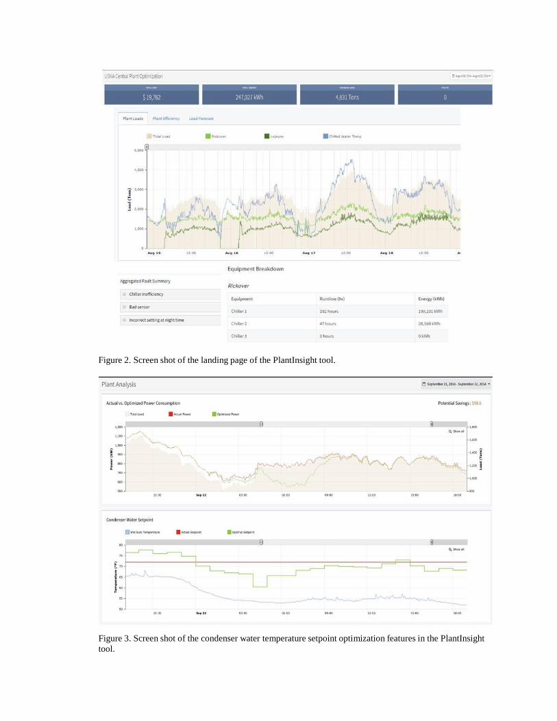
Figure 2. Screen shot of the landing page of the PlantInsight tool.

Figure 3. Screen shot of the condenser water temperature setpoint optimization features in the PlantInsight

tool.

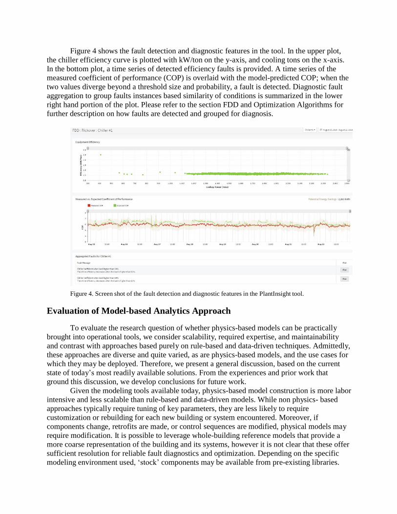
Figure 4 shows the fault detection and diagnostic features in the tool. In the upper plot,

the chiller efficiency curve is plotted with kW/ton on the y-axis, and cooling tons on the x-axis.

In the bottom plot, a time series of detected efficiency faults is provided. A time series of the

measured coefficient of performance (COP) is overlaid with the model-predicted COP; when the

two values diverge beyond a threshold size and probability, a fault is detected. Diagnostic fault

aggregation to group faults instances based similarity of conditions is summarized in the lower

right hand portion of the plot. Please refer to the section FDD and Optimization Algorithms for

further description on how faults are detected and grouped for diagnosis.

Figure 4. Screen shot of the fault detection and diagnostic features in the PlantInsight tool.

Evaluation of Model-based Analytics Approach

To evaluate the research question of whether physics-based models can be practically

brought into operational tools, we consider scalability, required expertise, and maintainability

and contrast with approaches based purely on rule-based and data-driven techniques. Admittedly,

these approaches are diverse and quite varied, as are physics-based models, and the use cases for

which they may be deployed. Therefore, we present a general discussion, based on the current

state of today’s most readily available solutions. From the experiences and prior work that

ground this discussion, we develop conclusions for future work.

Given the modeling tools available today, physics-based model construction is more labor

intensive and less scalable than rule-based and data-driven models. While non physics- based

approaches typically require tuning of key parameters, they are less likely to require

customization or rebuilding for each new building or system encountered. Moreover, if

components change, retrofits are made, or control sequences are modified, physical models may

require modification. It is possible to leverage whole-building reference models that provide a

more coarse representation of the building and its systems, however it is not clear that these offer

sufficient resolution for reliable fault diagnostics and optimization. Depending on the specific

modeling environment used, ‘stock’ components may be available from pre-existing libraries.

However the models must then be adapted for use with specific diagnostic algorithms. For

example, in this work, the chiller model from the Modelica Buildings Library was adapted and

modified for use in the state/parameter estimation phase of the fault detection algorithm.

Model calibration requires a significant degree of specialized expertise in building

modeling, operations, and building science. In general however, it can largely be conducted with

data that is commonly available from building control systems. As in the case of rule-based and

data-driven models, the required data often needs to be cleansed to fill gaps and filter extreme or

erroneous values. Cost effective integration of control system data into analytics tools remains

one of the most significant challenges to advancing the state of today’s technology, whether

model-based or data-driven approaches are employed. In principle it is possible, but in practice

the associated cost and complexity often outweigh the benefits of the advanced analytics that

require the data integration. Once the data is obtained, care must be taken to ensure that the

models are being calibrated in a physically meaningful way. Auto-calibration routines that codify

some of the expertise that is needed for successful calibration are being developed by

researchers, and are beginning to be offered to the industry (Sanyal 2014; Sun 2016). However,

calibration approaches must be matched to the application. For example, calibration of a model

used for a chiller fault detection as it operates through dynamic and steady state regimes may be

quite different from that of a whole-building model that is used to determine faults in centralized

HVAC systems. Finally, the questions of when to recalibrate and how to account for faults

present in the calibration data are the subjects of ongoing research.

As described in the Introduction, in theory, model-based approaches offer the potential for enhanced diagnostic power. PlantInsight permits detection of periods of low chiller efficiency

that may be difficult to detect purely with data-driven approaches that are limited only to historic

data. In general however, more research is needed to validate whether model-based fault

detection, in practice, is more or equally effective than data-driven techniques. Finally, one can

consider the infrastructural aspects of practically delivering model-based approaches for use in

continuous operational analytics. The infrastructural requirements for such systems do not

present a practical challenge for scaled delivery. Cloud-based software services dominate today’s

solutions for operational analytics tools, precisely because of the cost-efficient, scalable,

computational and hosting flexibility that they provide.

Conclusions, Future Work

This paper presented the development of a physical model-based FDD and optimization

tool for a cooling plant. One conclusion on this work is that this approach is still cumbersome

given all of the steps to build and calibrate the model for ongoing operational use. With further

research to automatically calibrate and construct models, these types of tools could be made

more ready for production use. These physics-based techniques remain a compelling direction

for the continuous commissioning, optimization and FDD systems of the future. One major

advantage of a physics based models over data-driven models is the ability to extend them for

retrofit analysis as well as those that focus on operational efficiency analysis. One can drop in

new chillers, towers, or pumps and use the model for further analysis beyond the realm of prior

historic operations. In addition, how the system should operate can be compared to how it has

operated in the past.

Scaled delivery of these approaches will require a change in industry capacity and

expertise, as well as continued research and development to lower the bar of expertise that is

required. Today’s building energy analytics providers tend to have in-house data scientists, rather

than the building scientists who are currently needed to work with these complex models. We

also need to demonstrate the costs and benefits of these tools, and their advantages, to build

market demand. Ideally, physics-based models will be used throughout the building life cycle –

from design, to initial commissioning, to ongoing operations, valuation of proper maintenance,

and retrofit exploration. Even if these approaches are costly and complex if used solely for

identifying and diagnosing waste and efficiency opportunities, there is certainly a role for model-

based approaches in holistic strategies for advanced, efficient building operation. The building

energy analysis community is only beginning to have tools to deliver energy-aware transactive

controls and dynamic, anytime optimization – capabilities that will surely be needed in the

buildings and energy supply systems of the future.

Future research will explore auto-calibration techniques for diverse types and

applications of system and whole-building-level physical models. Solutions to automate and

simplify the creation of physics-based models based on existing specifications, drawings, and

building information models (BIM) are also needed for practical scalability. If the BIM vision

were successful, and coupled with information on sequences of operations, one could generate

digital specifications in a format that was interoperable with energy analysis tools. The next

stage for greater tool interoperability would be the capability to automatically import trend log

data to a model calibration routine. The development of standard, open FDD algorithms could

ensure that algorithms, models, and calibration routines can be seamlessly integrated. Finally,

there is a need for auto-correction and auto-tuning of controls based on the outputs of FDD

algorithms. Most of today’s systems either optimize controls or perform FDD, but it is rare to

close the loop by connecting the two. While not yet practical for deployment in today’s

buildings, these model-based systems are important for the eventual delivery of truly optimal

building performance.

Acknowledgement This work was supported by the Assistant Secretary for Energy Efficiency and Renewable

Energy, Building Technologies Office, of the U.S. Department of Energy under Contract No.

DE-AC02-05CH11231. Development of the PlantInsight tool was conducted under funding from

the U.S. Department of Defense’s Environmental Security Technology

Certification program, and with the generous participation of the operations staff at the US Naval

Academy. The authors thank the following team members who contributed to this research over

its duration – Sen Huang, Daniel McQuillen, Oren Schetrit, Michael Sohn, Michael Spears,

Michael Wetter, and Wangda Zuo.

References Bonvini, M., Piette, M.A., Wetter, M., Granderson, J., and Sohn, M. 2014. “FDD Bridging the

gap between simulation and the real world: An application to FDD.” Proceedings of the 2014

ACEEE Summer Study on Energy Efficiency in Buildings: (11)25-35. Bonvini, M., Sohn, M., Granderson, J., Wetter, M., and Piette, M.A. 2014. “Robust on-line fault

detection and diagnosis for HVAC components based on nonlinear state estimate

techniques.” Applied Energy 124:156-166. Granderson, J. and Lin, G. 2016. “Building energy information systems: Synthesis of costs,

savings, and best-practice uses.” Energy Efficiency, Online 19 February 2016: 1-16. Granderson, J., Piette M.A., and Ghatikar, G. 2011. “Building energy information systems: User

case studies.” Energy Efficiency 4(1): 17-30. Huang, S., and Zuo, W. 2014. “Optimization of the Water-Cooled Chiller System Operation.”

Proceedings of 2014 ASHRAE/IBPSA-USA Building Simulation Conference, Atlanta, GA,

United States, September 10-12: 300-307 Julier, S.J. and Uhlmann, J.K. 1996. “A general method for approximating nonlinear

transformations of probability distributions.” Robotics Research Group Technical Report,

Department of Engineering Science, University of Oxford: 1–27. Katipamula, S, Brambley, M. 2005. Methods for fault detection, diagnostics, and prognostics for

building systems – A review, part I.” HVAC&R Research. 11(1): 3–25. Pang, X., Wetter, M., Bhattacharya, P., and P. Haves. 2012. “A Framework for Simulation-based

Real-time whole building performance assessment.” Building and Environment, Volume

54:100-108. Sanyal, J., New, J.R., Edwards, R.E. and Parker, Lynne E. 2014. "Calibrating Building Energy

Models Using Supercomputer Trained Machine Learning Agents." Journal on Concurrency

and Computation: Practice and Experience, (26)13:2122-2133. Sun, K., Hong, T., Taylor-Lange, S., and Piette, M.A. 2016. “A Pattern-based Automated

Approach to Building Energy Model Calibration.” Applied Energy, Vol. 165, 1 March 2016:

214-224.

Wetter, M. 2001. “GenOpt – a generic optimization program.” Proceedings of the 7th

IBPSA

conference, Rio de Janeiro, Brazil: 601–8. Wetter, M., Zuo, W., Nouidui, T. S., and Pang, X. 2014. “Modelica Buildings Library.”

Journal of Building Performance Simulation, 7(4):253-270.