Policy Research Working Paper 8975

Can Taxes Help Ensure a Fair Globalization?François LangotRossana Merola

Samil Oh

Poverty and Equity Global Practice August 2019

Pub

lic D

iscl

osur

e A

utho

rized

Pub

lic D

iscl

osur

e A

utho

rized

Pub

lic D

iscl

osur

e A

utho

rized

Pub

lic D

iscl

osur

e A

utho

rized

Produced by the Research Support Team

Abstract

The Policy Research Working Paper Series disseminates the findings of work in progress to encourage the exchange of ideas about development issues. An objective of the series is to get the findings out quickly, even if the presentations are less than fully polished. The papers carry the names of the authors and should be cited accordingly. The findings, interpretations, and conclusions expressed in this paper are entirely those of the authors. They do not necessarily represent the views of the International Bank for Reconstruction and Development/World Bank and its affiliated organizations, or those of the Executive Directors of the World Bank or the governments they represent.

Policy Research Working Paper 8975

This paper analyzes whether taxation can be successfully used to reduce the incidence of labor informality and achieve higher equality in a globalized economy. To this purpose, it develops a two-area model: a developed country and an emerging country. The two areas differ according to the size of the informal sector, which is characterized by a more flexible labor market and lower productivity. To illustrate the potential role of taxation in achieving a more fair income distribution, the paper introduces a trade shock to simulate the effects of trade liberalization. Trade expansion has often been blamed for leading to an expan-sion of the informal sector and a widening of wage income

disparities. In this context, the paper analyzes whether a budget-neutral tax reform—switching the tax burden from payroll taxes paid by firms operating in the formal sector to a consumption tax—can mitigate possible adverse effects of trade liberalization and support labor formalization. The effects of taxation are seen in the context of the trade-offs between growth, labor formality and equity. The analysis suggests that small improvements in formalization, result-ing from the tax reform, come at the cost of widening income inequality. To reduce the incidence of low-quality jobs, tax policy interventions should go hand in hand with more effective social protection systems and labor laws.

This paper is a product of the Poverty and Equity Global Practice. It is part of a larger effort by the World Bank to provide open access to its research and make a contribution to development policy discussions around the world. Policy Research Working Papers are also posted on the Web at http://www.worldbank.org/prwp. The authors may be contacted at merola@ilo.org.

Can taxes help ensure a fair globalization? ∗

François Langot† Rossana Merola‡ Samil Oh

∗Funding from the World Bank-ILO Research Fund is gratefully acknowledged. The work greatly ben-eted from helpful comments by Stéphane Adjemian, Thomas Brand, Matteo Cacciatore, Valerie Cerra,Ralph Chami, Olivier Charlot, Ekkehard Ernst, Aurelien Eyquem, Miguel Foguel, Fabio Ghironi, Jinill Kim,Stefan Kühn, Gladys Lopez-Acevedo, Hugo Ñopo, Pierella Paci, Ugo Panizza, Stela Rubinova, RaymondSaner, Thepthida Sopraseuth, Christian Viegelahn, Sergio Vieira, the DYNARE team, as well as partici-pants in seminars and conferences at the World Bank, the ILO, the Graduate Institute of International andDevelopment Studies in Geneva, the International Labour and Employment Relations Association (ILERA)2018 Congress, the 2018 Asian Meeting of Econometric Society, the 2019 Congress of the Swiss Society ofEconomics and Statistics and the EcoMod 2019 Conference. However, all errors remain our own. The viewscontained here are ours own and not necessarily those of the ILO and the World Bank Group.†Le Mans University (Gains-TEPP & IRA), Paris School of Economics & Cepremap. E-mail:

angot@univ-lemans.fr‡ILO, International Labour Oce, Research Department. E-mail: merola@ilo.orgBank of Korea, Research Department. E-mail: samil.oh@bok.or.kr

Contents

1 Introduction 1

2 Model 3

2.1 Households . . . . . . . . . . . . . . . . . . . . . . . . . . . . . . . . . . . . 42.2 Production . . . . . . . . . . . . . . . . . . . . . . . . . . . . . . . . . . . . 6

2.2.1 Intermediate goods . . . . . . . . . . . . . . . . . . . . . . . . . . . . 72.2.2 Final goods . . . . . . . . . . . . . . . . . . . . . . . . . . . . . . . . 10

2.3 Government . . . . . . . . . . . . . . . . . . . . . . . . . . . . . . . . . . . . 132.4 Closing conditions . . . . . . . . . . . . . . . . . . . . . . . . . . . . . . . . . 13

3 Calibration 14

4 The impact of trade liberalization 17

5 Tax reform 22

6 Conclusions 27

A Dynare equations 34

B Steady states 37

2

List of Figures

1 The nal good sector . . . . . . . . . . . . . . . . . . . . . . . . . . . . . . . 192 The labor market . . . . . . . . . . . . . . . . . . . . . . . . . . . . . . . . . 233 Unemployment . . . . . . . . . . . . . . . . . . . . . . . . . . . . . . . . . . 244 Wage inequality . . . . . . . . . . . . . . . . . . . . . . . . . . . . . . . . . . 375 Goods markets . . . . . . . . . . . . . . . . . . . . . . . . . . . . . . . . . . 386 Labor markets . . . . . . . . . . . . . . . . . . . . . . . . . . . . . . . . . . . 397 Unemployment . . . . . . . . . . . . . . . . . . . . . . . . . . . . . . . . . . 40

List of Tables

1 Calibration . . . . . . . . . . . . . . . . . . . . . . . . . . . . . . . . . . . . 16

3

1 Introduction

In the three decades prior to the global nancial crisis, household income inequality increasedin a large majority of OECD countries. Emerging countries have income inequality signi-cantly higher than the OECD average, although some countries (such as Brazil, Indonesiaand, on some indicators, Argentina) have recorded signicant progress in reducing inequalityover the past 20 years (OECD, 2011).

In addition, during the late 20th century there was a general increase in the informaleconomy in many countries around the world (see Schneider and Enste (2000)). Heintz andPollin (2005), for example, show that within a data set of 23 countries, 19 showed increasesin informality. Similarly, ILO data show that from 2002 self-employment increased in alldeveloping regions, and world-wide it increased from about one-quarter to one-third of non-agricultural employment during 1980-2000 (ILO, 2013). The high incidence of informalityis an issue of concern especially in developing countries, where on average, more than 50percent of the labor force is informal.1

Among the drivers of rising informality, the conventional view blames trade liberalizationfor being responsible for the fall in wages for unskilled and low-income workers, as well as therise in informal and less protected forms of employment. Therefore, despite its uncontrover-sial expansionary eects on global growth, trade expansion has not always been translatedinto more equal incomes and better working conditions.2

In these circumstances, an ecient tax system is indeed an important tool for addressingrising inequality and informality and restoring robust economic growth. On the one side,taxation is a powerful policy tool to redistribute income and make the post-tax incomedistribution less unequal. On the other side, taxation is a potential tool to lessen the costs ofoperating in the formal sector, since formality choices are very elastic to marginal tax rates.Indeed, a targeted and well-balanced tax code is an essential element in making furtherprogress in achieving the Sustainable Development Goals by providing a stable funding basefor high-quality public services for all and eective transfers targeted to those most in need.

In this context, our analysis contributes to the literature by investigating whether tax-ation may be an ecient policy tool to support labor formalization in a globalized econ-omy without widening income disparities. Our analysis is based on a Dynamic StochasticGeneral Equilibrium (DSGE) model with two asymmetric countries: a developed and anemerging country. These two countries dier according to the size of the informal sector inthe intermediate-good sector. The informal sector is characterized by a more exible labormarket (i.e. rapid entry and exit and more exible adjustment to change in demand) andlower productivity. In this respect, our paper relates to the recent theoretical literature em-bedding the informal sector in DSGE models (e.g. Conesa et al. (2002), Busato and Chiarini(2004), Orsi et al. (2014), Pappa et al. (2015), Dellas et al. (2017)). Within this strand

1In many Latin American countries informal employment exceeds 50 percent of total urban labor force(Gasparini and Tornarolli (2007)). Estimates for Sub-Saharan Africa and Asia are even higher (Jütting etal. (2008)). For an overview on job quality in emerging economies, see OECD (2015).

2For a more comprehensive discussion, see Bacchetta et al. (2009).

1

of literature, very few works enrich DSGE models with both informality and a fully-edgedlabor market with search and matching frictions. The few exceptions, to the best of ourknowledge, are Cook and Nosaka (2005), Zenou (2008), Satchi and Temple (2010), Batiniet al. (2011), Colombo et al. (2018), Bosch and Esteban-Pretel (2015) for Mexico, Anandand Khera (2016) for India and Poirier and Trupkin (2018) for Argentina. However, most ofthe aforementioned theoretical works have a dierent focus and very often analyze the roleof regulation, while none of them analyzes the eect of taxation on informality. In addition,models developed in the aforementioned studies describe closed economies and none of themis suitable to analyze the impact of policies in a globalized economy from both a developedand a developing country perspective.

The novelty of our paper is to focus on the role of taxation in reallocating labor betweenformal and informal activities in countries which participate in international trade. The ef-fects of taxation are seen in the context of the trade-os between growth, labor formality andequity. We start from a model à la Melitz (2003) and we extend it in two directions. First,we propose a dynamic model as in Ghironi and Melitz (2005), with search and matchingfrictions as in Helpman, Itskhoki and Redding (2010) and Cacciatore and Ghironi (2015).Second, we distinguish two asymmetric areas, a developed and an emerging country, charac-terized by dierent incidence of informality. We model informality as proposed by Charlot,Malherbet and Terra (2015)3 in a closed economy static model. Our model closely followsCacciatore and Ghironi (2015). However, Cacciatore and Ghironi (2015) focus on developedeconomies where a representative agent can be employed in only one sector, the presence ofinformality being not considered. In order to fully capture the impact of a tax reform inemerging economies, it seems to be crucial to model the interplay between the formal andinformal sectors. Therefore, our main contribution is that we embed the informal sector,as we believe that the analysis of labor market dynamics cannot be limited solely to theformal sector, given the high incidence of informality especially in developing and emergingcountries. Furthermore, in order to assess whether a scal reform can enable transition toformalization, we add taxation as well as hand-to-mouth agents in the model, which is notembedded in Cacciatore and Ghironi (2015).

Our work is related to the literature analyzing the impact of taxation on informality. Em-pirical evidence points out that reducing taxation on formal businesses eases the migrationof entrepreneurs from the informal to the formal sector, where productivity is higher, withpositive eect on output and economic eciency (see Slonimczyk (2012) for the Russian Fed-eration and Araujo and Rodrigues (2016) for Brazil). Higher tax rates among rm-ownersinduce not only substantial movements to the informal sector, but also under-reporting oftaxable earnings and income shifting to tax-favored business forms, which may ultimatelylead to inecient allocation or resources (see Waseem (2018) for an analysis of the Pakistanitax reform introduced in 2009). If informality is voluntary, lower taxation rates should reducerms' incentives to enter the informal sector. However, even if informality is involuntary,lower tax rates could reduce informality by encouraging formal sector rms to expand em-

3These authors limit their analysis to a closed economy static model.

2

ployment and create more formal jobs. This strand of the literature suggests that the bestapproach to reduce the size of the informal sector is using taxation to reduce the costs ofbeing formal and create the right incentives for companies and workers intending to switchto the formal sector. However, dierent tax instruments may have dierent eects in pro-moting the transition to the formal economy. For instance, lower taxes on social securitycontributions or on capital translates to a lower degree of informality, whereas cutting taxeson labor income has the opposite eect. Reducing personal income taxes increases grosswages, thus making the informal sector which is labor intensive more attractive.

Our analysis highlights a number of interesting results. We start by introducing a tradeshock which simulates the eect of trade liberalization in a globalized economy. Simulationsin our model point out that in the short term trade liberalization boosts economic activityand employment in both the formal and informal sectors. However, this employment ex-pansion is biased toward the informal sector, which is not subject to labor regulation andhence is more exible. In addition, in the long run after the strong employment gainsrecorded during the initial phase of trade expansion there is a phase characterized by acontraction on the labor market. We then investigate whether it is possible to correct thisbias in favor of the informal sector by reducing payroll taxes paid by rms operating in theformal sector. This policy exercise simulates the eects of several programs implemented inemerging economies (e.g. SIMPLES and SUPERSIMPLES in Brazil and the Monotax inArgentina) aiming at reducing the tax burden for small enterprises which are more likely tooperate in the informal sector.4 We show that an increase of the consumption tax could bea relevant strategy to nance the payroll tax cuts. Although this budget-neutral tax reformsupports the formalization process on the labor market, we observe that small improvementsin formalization come at the cost of widening income inequality.

The rest of the paper is structured as follows. In Section 2 we describe the model, whilein Section 3 we discuss the calibration. In Section 4 we introduce the trade shock to simulatethe eect of trade liberalization. The impact of a budget-neutral tax reform is discussed inSection 5. Finally, Section 6 concludes. Some technical aspects are reported in the Appendix.

2 Model

We develop a two-country model, calibrated on a developed and an emerging country. Thetwo economies are modeled exactly symmetrically, so that the following description in thisSection holds for both economies. We assume a dual labor market, with formal and informalworkers. The two countries dier for the incidence of labor informality, since emerging coun-tries are characterized by higher informality than advanced economies. Variables appearingwith an asterisk refer to the modeled foreign economy.

4These types of programs, such as microcredit and tax reliefs for small enterprises, have been blamed forlimiting growth opportunities in emerging economies, since they increase the incentives for small enterprisesto remain small (see Hsieh and Olken (2014)). For an analysis on the diculties of Brazilian small rms tosurpass the threshold of medium-size plants, see Coelho et al. (2017).

3

There are four actors in each country: households, rms producing intermediate goods,rms producing nal goods and the government. The model features heterogeneous house-holds: Ricardian and non-Ricardian. Ricardian households hold bonds but do not supplylabor, whereas non-Ricardian households do not have access to nancial markets to nancetheir consumption needs. Therefore, non-Ricardian households need to supply labor in orderto nance their consumption needs. Since recent evidence shows that there is no segmen-tation between the formal and the informal sector (see Charlot et al. (2015)), we assumethat workers can move between the two sectors.5 They may decide to either supply laborin the formal sector, or supply labor in the informal sector or be unemployed. Labor ishence supplied only by non-Ricardian households to intermediate good producers. Inter-mediate good producers operate in a perfect competitive market and hire labor either onthe formal or informal market to produce intermediate goods which are sold to nal goodproducers. Final good producers combine intermediate goods into a nal good which is soldon a monopolistically-competitive market.6 Finally, to provide public goods and unemploy-ment benets, the government collects taxes paid on consumption by all households as wellas payroll taxes paid only by employees and employers (i.e. intermediate good producers)operating in the formal sector.

For the sake of simplicity, the model does not feature nominal price rigidities and goodsare produced using only labor without capital.

2.1 Households

There are two types of households in the economy: Ricardian and non-Ricardian. Ricardianhouseholds (indexed by a) do not work, hold assets and have access to international nancialmarkets. Non-Ricardian households supply labor, but have no access to nancial markets.Non-Ricardian households can work in the formal sector (indexed by F ), work in the informalsector (indexed by I) or being unemployed (indexed by u).

For all agents, the consumption basket Ct aggregates Home and Foreign consumption ina Dixit-Stiglitz form:

Ct =

[∫ 1

0

Ct(i)φ−1φ di

] φφ−1

(1)

5For the sake of simplicity, we focus only on labor informality and we abstract from business informality,i.e. we abstract from modeling how rms can switch from the formal to the informal sector and vice versa.Chacaltana et al. (2018) show that business informality does not imply labor informality and vice versa.The decision of a rm to go formal is the product of a complex evaluation based not only on the tax burdenbut also on other factors, such as the opportunity to have access to credit. Modeling rms' choice to switchbetween the formal and informal sector would require embedding the nancial sector into the model, whichwill pose challenges to the analytical manageability of the model. Becker (2018) provides an example of amodel featuring a sector-switching mechanism.

6The distinction between formal and informal labor arises only for rms producing intermediate goodswhich are used by nal good producers as the sole input. Intermediate good producers are not allowed todirectly export abroad. This assumption is needed because exporting means some minimal formality andrespect of customs requirements and are more subject to control and customs inspection.

4

where φ > 1 is the symmetric elasticity of substitution across goods. The correspondingconsumption-based price index, Pt, is given by:

Pt =

[∫ 1

0

Pt(i)1−φdi

] 11−φ

(2)

Ricardian agents smooth their consumption, Cat, over time and thus maximize the life-time utility function E0

∑∞t=0 β

t[

(Cat)1−γc

1−γc

], where γ is the risk aversion parameter and β is

the discount factor. Utility maximization is subject to the following budget constraint:

At+1 + StA∗t+1 + Pt

ψ

2

(At+1

Pt

)2

+ StP∗t

ψ

2

(A∗t+1

P ∗t

)2

+ (1 + τ ct )PtCat

= (1 + iNt )At + (1 + i∗Nt )A∗tSt + Pt(TAt + T it + T ft )

Ricardian agents hold domestic assets At (denominated in domestic currency) on which theyreceive the nominal interest rate iNt and foreign assets A∗t+1 (denominated in foreign currency)on which they receive the interest rate i∗Nt . Assets are subject to quadratic adjustment costs,measured by the parameter ψ . These costs are paid to nancial intermediaries whose onlyfunction is to collect these transaction fees and rebate the revenue to households in lump-sumfashion in equilibrium. Ricardian households pay a consumption tax τ ct on their consumptionCat . St is the nominal exchange rate. Moreover, TAt is a lump-sum rebate of costs of adjusting

asset holdings from the intermediaries to which it is paid and T it and T ft are a lump-sumrebate of prots from intermediate and nal goods production.78

If we denote At+1

Pt= at+1 and

A∗t+1

P ∗t

= a∗t+1, we can re-write the budget constraint in realterms:

at+1 +Qta∗t+1 +

ψ

2(at+1)2 +Qt

ψ

2

(a∗t+1

)2+ (1 + τ ct )Cat

=(1 + iNt )

1 + πtat +

(1 + i∗Nt )

1 + π∗tQta

∗t + TAt + T it + T ft

where πt is the ination rate and 1 + πt = PtPt−1

. The term Qt = StP∗t /Pt stands for the real

exchange rate. If we dene the domestic and foreign gross real interest rates as 1+it =(1+iNt )

1+πt

and 1 + i∗t =(1+i∗Nt )

1+π∗t, we can re-write the budget constraint as:

at+1+Qta∗t+1+

ψ

2(at+1)2+

ψ

2Qt

(a∗t+1

)2+(1+τ ct )Cat = (1+it)at+(1+i∗t )a

∗tQt+T

At +T it+T

ft (3)

7We assume that Ricardian households are rms' owners.8The denition of this set of lump-sum rebate of costs and prots is the same as in Cacciatore and

Ghironi (2015) and hence we refer to their paper for a complete derivation of these variables. The onlydierence in our model concerns the lump-sum rebate of prots from intermediate goods, which is dened

as: T it = Pt

(φtZFtlFt − wFt

PtlFt − wIt

PtlIt − κFVFt − κIVIt

).

5

where it and i∗t are respectively the real interest rates on domestic and foreign assets.The Euler equations for domestic and foreign asset holding are respectively:

(1 + ψat+1) = (1 + it+1)βEt

(C−γcat+1

C−γcat

1 + τ ct1 + τ ct+1

)(4)

(1 + ψa∗t+1) = (1 + i∗t+1)βEt

(C−γcat+1

C−γcat

Qt+1

Qt

1 + τ ct1 + τ ct+1

)(5)

On the other hand, non-Ricardian households do not have access to nancial marketsand hence they can nance their consumption needs either though labor income (wFt if theysupply labor to the formal sector and wIt if they supply labor to the informal sector) orthrough unemployment benets (bt) if they do not work.

The following equations dene non-Ricardian agents' consumption depending on whetherthey work in the formal sector, or they work in the informal sector, or they are unemployed:

CFt =(1− τwt )

(1 + τ ct )wFt lFt (6)

CIt =wIt

(1 + τ ct )lIt (7)

Cut =bt

(1 + τ ct )(1− lt) (8)

The payroll tax on employees, τwt , is borne only by non-Ricardian agents employed inthe formal sector. Total labor supply, lt, is the sum of labor supplied by non-Ricardianhouseholds in the formal and informal sectors, i.e. lt = lFt + lIt. In equilibrium, aggregateunemployment is given by:

Ut = 1− lFt − lIt (9)

Total consumption Ct is dened as the weighted sum of consumption of Ricardian house-holds (Cat) and non-Ricardian households working in the formal sector (CFt), in the informalsector (CIt) or unemployed (Cut):

Ct = ωCat + (1− ω)(CFt + CIt + Cut) (10)

where ω is the share of Ricardian households.

2.2 Production

There are two vertically integrated production sectors. In the upstream, in both the formaland the informal sector, intermediate goods are produced in perfect competition using onlylabor. Intermediate goods are then sold to nal good producers. In the downstream, eachsector i is populated by a representative monopolistically competitive multi-product rm,which uses intermediate goods as inputs to produce dierentiated varieties. In equilibrium,some of these varieties are exported while others are sold only on the domestic market.

6

2.2.1 Intermediate goods

We assume a unit mass of intermediate good producers, which operate both in the formaland informal sectors. Both sectors are subject to search and matching frictions as in theDiamond-Mortensen-Pissarides framework. Unemployed agents search for a job in bothsectors and search eorts are endogenous. Wages are set through an individual bargainingprocess.

We assume a constant-return-to-scale matching technology in each sector j, for j = F, I,where F and I refer respectively to the formal and the informal sector. The matchingtechnology converts aggregate unemployed workers, Ut, and aggregate vacancies, Vt, intoaggregate matches, Mt. The matching rate in each j sector is:

Mjt = χj(ejtUt)1−εV ε

jt (11)

where Ut is the total number of unemployed workers and Vt is the number of vacancies. Theparameters χ and ε measure respectively the matching eciency and the matching functionelasticity, with χ > 0 and 0 < ε < 1. Let ejt denote search eorts for the job type j whenagents are unemployed.

The job lling rate, qt, is:

qjt =Mjt

Vjt= χj

(ejtUtVjt

)1−ε

(12)

The job nding rate, ι is:

ιjt =Mjt

Ut= χj

(VjtejtUt

)εejt (13)

As in Krause and Lubik (2007), we assume that newly created matches become productiveonly in the next period. The law of motion of employment, ljt, is:

ljt = (1− λj)ljt−1 + qjt−1vjt−1 (14)

where λj ∈ (0, 1) is the exogenous separation rate and vjt is the number of vacancies postedby the rm in period t. In equilibrium vjt = Vjt.

Firms, both in the formal and informal sector, hire labor lt to produce an intermediategood yjt according to the following technology :

yIntjt = Zjtljt ∀ j = F, I (15)

where Zjt is an exogenous technology term which follows an autoregressive process AR(1):

logZjt = φZ1 logZjt−1 + φZ2 logZ∗jt−1 + εZjt. (16)

7

In both sectors j = F, I, intermediate rms choose the number of vacancies, vjt, andemployment, ljt, to maximize the discount value of their prots:

E0

∞∑t=0

βtuC,tuC,0

(ϕtZjtljt − wjtljt(1 + τ fjt)− κjvjt

)(17)

subject to the law of motion for labor: ljt = (1 − λj)ljt−1 + qjt−1vjt−1, where ϕt is the realprice at which intermediate goods producers sell their goods to nal good producers and itis expressed in units of consumption9; wFt is the wage paid to workers in the formal sector(lFt), while wIt is the wage paid to workers in the informal sector (lIt). In both sectors,intermediate good producers incur a cost of κj units of consumption per vacancy postedvjt. The term τ fjt represents a payroll tax on employers. These taxes are paid only by rmsoperating in the formal sector. Hence τ fF t > 0, whereas τ fIt = 0.

The rst order conditions (hereafter, FOCs) on vjt and ljt in the formal and informalsector are respectively:

κjqjt

= Et [βt,t+1µjt+1] (18)

µjt = ϕjtZjt − wjt(1 + τ fjt) + Et [βt,t+1(1− λj)µjt+1] (19)

where µjt is the Lagrangian multiplier for labor adjustment and measures the current valueof an additional worker. Combining both FOCs leads to the job creation conditions in bothsectors:

κFqFt

= Et

βt,t+1

[(1− λF )

κFqFt+1

+ ϕt+1ZFt+1 − wFt+1(1 + τ fF t+1)

](20)

κIqIt

= Et

βt,t+1

[(1− λI)

κIqIt+1

+ ϕt+1ZIt+1 − wIt+1

](21)

where βt,t+1 ≡ βuC,t+1

uC,tis the one period ahead stochastic discount factor.

For both the formal and the informal sector, the job creation conditions state that, inequilibrium, the vacancy creation cost incurred by the rm per current match is equal to theexpected discounted value of the vacancy creation cost per future match, further discountedby the probability of current match survival 1− λ, plus the prots from the match at timet. Prots from the match take into account the future marginal revenue product from thematch and its wage cost.

Wages Nominal wages are set through an individual Nash bargaining process. In eacht period and in both sectors J = F, I, the real value of an existing, productive match fora producer, Jt, is the sum of the marginal product of the match (ϕtZjt) and the expecteddiscounted continuation value of the match (Etβt,t+1(1− λj)Jjt+1), net of the wage bill:

Jjt = ϕtZjt − wjt(1 + τ fjt) + Etβt,t+1(1− λj)Jjt+1 (22)

9Firms are owned by households and uC,t is the marginal utility of consumption. This ensures that rstorder conditions are measured in the same units.

8

The worker's value of being matched, in both the formal and informal sector, is given bythe sum of real wage received and the expected discounted future value of being matched bythe rm:

Wjt =(1− τwjt)(1 + τ ct )

wjt + Etβt,t+1[(1− λj)Wjt+1 + λjUu,t+1] (23)

The expected future value of being matched by the rm (the last term on the right-handside of Eq.(23)) is a weighted average of probability 1− λ that the match will survive or theprobability λ that the worker will become unemployed.

The value of being unemployed is dened as:

Ut =bt

(1 + τ ct )−ϑ e

1+%Ft

1 + %−ϑ e

1+%It

1 + %+Etβt,t+1[ιFtWFt+1 +ιItWIt+1 +(1−ιFt−ιIt)Uu,t+1] (24)

where ϑe1+%jt

1+%is a convex search cost and % is the elasticity of disutility of searching. Therefore,

the value of being unemployed is the sum of unemployment benets10 net of search costs and the expected discounted future value of future states, where ιFt and ιIt are the probabilityof becoming employed respectively in the formal or informal sector.

We dene worker's surplus Hjt ≡ Wjt−Ut. The worker surplus in the formal and informalsector is given by:

HFt =(1− τwjt)(1 + τ ct )

wjt −(

bt(1 + τ ct )

− ϑ e1+%Ft

1 + %− ϑ e

1+%It

1 + %

)+ (1− λF − ιFt − ιIt)Et(βt,t+1HFt+1)

(25)

HIt =wIt

(1 + τ ct )−(

bt(1 + τ ct )

− ϑ e1+%Ft

1 + %− ϑ e

1+%It

1 + %

)+ (1− λI − ιFt − ιIt)Et(βt,t+1HIt+1) (26)

Nash bargaining maximizes the joint surplus JηjtH1−ηjt with respect to wjt, where Hjt and

Jjt stand for surpluses respectively for workers and rms and the parameter η measures thebargaining power of rms. The FOC implies:

ηHjt∂Jjt∂wjt

+ (1− η)Jjt∂Hjt

∂wjt= 0 (27)

where ∂Jjt∂wjt

= −(1 + τ fjt) and ∂Hjt∂wjt

=1−τwjt1+τct

. Hence, the sharing rule can be rewritten in thefollowing form:

(1 + τ fjt)ηHjt =1− τwjt1 + τ ct

(1− η)Jjt (28)

10We assume that the informal sector does not allow the worker to be eligible for the unemploymentbenets. Given that we have a representative unemployed worker, we set an average unemployment benets,bt = lFt/(lFt + lIt)bWFt, where the parameter b is the replacement rate and measures benet generosity bycomparing unemployment benets received when not working to wages earned when employed.

9

The bargained wage satises the following condition, respectively in the formal and informalsector:

wFt =η

1− τwFt

[bt

(1 + τ ct )− ϑ e

1+%Ft

1 + %− ϑ e

1+%It

1 + %

]+

1− η1 + τ fF t

ϕtZFt + Et

[βt,t+1JFt+1

((1− λF )− (1− λF − ιFt)

1 + τ fF t1 + τ fF t+1

1− τwFt+1

1− τwFt

)](29)

wIt = η

[bt

(1 + τ ct )− ϑ e

1+%Ft

1 + %− ϑ e

1+%It

1 + %

]+ (1− η) [ϕtZIt + ιItEt (βt,t+1JIt+1)] (30)

Wages are a linear combination determined by the bargaining power parameter η ofworker's outside option and the marginal revenue product generated by the worker plus theexpected discounted continuation value of the match to the rm. For high values of η, thebargaining power of rms is higher and the portion of the net marginal revenue product andcontinuation value to the rm appropriated by workers as wage payments is smaller, hencethe outside option becomes more relevant.

Optimal search intensities are given by ∂Ut/∂ejt = 0, which yields:

ϑe%jt =∂ιjt∂ejt

Et(βt,t+1Hjt+1) (31)

ϑe%Ft =

(1− ηη

)χF

(VFteFtUt

)ε( 1− τwt+1

(1 + τ ft+1)(1 + τ ct+1)

)κFqFt

(32)

ϑe%It =

(1− ηη

)χI

(VIteItUt

)ε(1

1 + τ ct+1

)κIqIt

(33)

This set of equations shows that search eorts are increasing in market tightness (Vjt/Ujt)

and decreasing in taxes. We dene the tax wedge as TWFt =1−τwt+1

(1+τft+1)(1+τct+1)in the formal

sector and TWIt =(

11+τct+1

)in the informal sector. Equations above show that the higher the

tax wedge, the lower the search eort. However, the tax wedge is not symmetrical betweensectors and hence the incentive to search for an informal job are reduced only by an increasein the consumption tax, τ ct , but they are not aected by changes in payroll taxes, τ ft and τwt .

2.2.2 Final goods

In this subsection variables denoted by the letter d refer to a country's own goods consumedor produced domestically, whereas x refers to quantities and prices of exports.

Producer i is a multi-product rm that produces a set of dierentiated product varieties,indexed by ω, y(ω, i), which is dened over a continuum Ω:

Yt(i) =

(∫ ∞ω∈Ω

yt(ω, i)θ−1θ dω

) θθ−1

(34)

10

where θ > 1 is the symmetric elasticity of substitution across varieties. To save notation,from now on, we omit the index i, since consumption-producing sectors are symmetric inthe economy.

We dene P yt , the cost of the product bundle Yt:

P yt =

(∫ ∞ω∈Ω

pyt (ω)1−θdω

) 11−θ

(35)

where pyt (ω) is the nominal marginal cost of producing variety ω.To create a new variety ω, each retailer needs to create a new plant, facing a sunk

investment, fe,t, denominated in units of intermediate input. Each plant produces usingdierent technologies indexed by relative productivity z(ω), which is drawn from a commondistribution G(z) with support on [zmin,∞). For the sake of simplicity, from now on weomit ω. This relative productivity level remains xed thereafter. Productivity level offoreign plants are drawn from an identical distribution. Each plant uses intermediate inputsto produce its dierentiated product variety, facing the real marginal cost:

ϕz,t ≡pyt (z)

PT=ϕtz

(36)

The number of products created and commercialized by each retailer is endogenous. Ateach point in time, only a subset of varieties Ωt ⊂ Ω is actually available to consumers.Therefore, at time t, each Home retailer commercializes Nd,t varieties and creates Ne,t newproducts that will be available for sale at time t+ 1. New and incumbent plants can be hitby a "death" shock with probability δ ∈ (0, 1) at the end of each period. The law of motionfor the stock of producing plants is:

Nd,t+1 = (1− δ)(Nd,t +Ne,t) (37)

where δ is the rm's exit rate. When serving the foreign market, each retailer faces per-uniticeberg trade costs, τt > 1, as well as xed export costs, fx,t paid for each exported productand denominated in units of intermediate input. We dene total xed costs fx,t = fx,tNx,t,where Nx,t denotes the number of product varieties exported abroad. If xed export costsare absent (fx,t = 0), each producer would nd it optimal to sell all its product varietiesboth domestically and abroad. Fixed export costs imply that only varieties produced byplants with suciently high productivity (above a cuto level zx,t, determined below) areexportable.

We dene two special average productivity levels (weighted by relative output shares):an average zd for all producing plants and an average zx,t for all exporting plants:

zd =

(∫ ∞zmin

zθ−1dG(z)

) 1θ−1

zx,t =

[1

1−G(zx,t)

](∫ ∞zx,t

zθ−1dG(z)

) 1θ−1

11

We assume that G(·) is Pareto with shape parameter kp > θ−1.11 As a result, zd = κ1θ−1 zmin

and zx,t = κ1θ−1 zx,t, where κ = kp/[kp − (θ − 1)]. The share of exporting plants is given by:

Nx,t = [1−G(zx,t)]Nd,t =

(zminzx,t

)−kpκ

kpθ−1Nd,t (38)

The real costs of producing the bundles Yd,t and Yx,t are respectively:

P yd,t

Pt= N

11−θd,t

ϕtzd,

P yx,t

Pt= N

11−θx,t

ϕtzx,t

(39)

The nal producer determines Nd,t+1 and the productivity cuto zx,t to minimize thepresent discount value of costs:

∞∑s=t

βt,s

[P yd,s

PsYd,s + τs

P yx,s

PsYx,s +

(Ns+1

1− δ−Ns

)fe,sϕs +Nx,sfx,sϕs

](40)

subject to (38), (39), and zx,t = κ1θ−1 zx,t.

The FOC with respect to zx,t yields:

τtP yx,t

Pt

Yx,tNx,t

=(θ − 1)kpkp − (θ − 1)

fx,tϕt (41)

In equilibrium, the marginal revenue from adding a variety with productivity zx,t to theexport bundle has to be equal to the xed cost. Thus, varieties produced by plants withproductivity below zx,t are distributed only in the domestic market. The composition ofthe traded bundle is endogenous and the set of exported products uctuates over time withchanges in the protability of export.

The FOC with respect to Nd,t+1 determines product creation:

ϕtfe,t = (1− δ)βt,t+1

ϕt+1

(fe,t+1 − Nx,t+1

Nd,t+1fx,t+1

)+ 1θ−1

(P yd,t+1

Pt+1

Yd,t+1

Nd,t+1+ τt+1

P yx,t+1

Pt+1

Yx,t+1

Nx,t+1

Nx,t+1

Nd,t+1

) (42)

In equilibrium, the cost of producing an additional variety, ϕtfe,t, must be equal to itsexpected benet, which includes expected savings on future sunk investment costs augmentedby the marginal revenue from commercializing the variety, net of xed export costs, if it isexported.

11Hence, G(x) =(

zzmin

)−kp

.

12

Domestic and export prices Let Pd,t and Px,t be the price of the product bundle Yd,tand Yx,t. Each nal producer faces the following domestic and foreign demand for its productbundles:

Yd,t =

(Pd,tPt

)−φY Ct , Yx,t =

(Px,tP ∗t

)−φY C∗t (43)

where Y Ct and Y C∗

t stand for aggregate demands of the consumption basket in the domesticand foreign country. The elasticity of substitution across sectoral bundles for the aggregatedemand, φ > 1, is equal to the elasticity of substitution for the consumption basket, al-though aggregate demand in each country includes sources other than consumption. Thisassumption ensures that the consumption price index for the the consumption aggregator isalso the price index for aggregate demand of the basket.

We assume producer currency pricing (PCP): nal producers set the price of the productbundle, Pd,t, and the the price of the export bundle, P h

x,t, in their own domestic currency,letting the price in the foreign market move with the nominal exchange rate, that is: Px,t =τP h

x,t/St. Because of xed export costs, the composition of domestic and export bundlesis dierent, and hence producers face dierent marginal costs of producing these bundles.Therefore nal producers set two dierent prices for the Home and Foreign markets. Theoptimal price for domestic sales and exported sales satises respectively:

Pd,tPt

=φ

φ− 1

P yd,t

Pt,

P hx,t

Pt=

τtQt

φ

φ− 1

P yx,t

Pt(44)

where Qt = StP∗t /Pt is the real exchange rate.

We dene the average price of a domestic variety, ρd,t ≡ N1θ−1

d,t (Pd,t/Pt) and the average

price of an exported variety, ρx,t ≡ N1θ−1

x,t (Px,t/P∗t ). Combining the equations (39) and (44),

we obtain the average price of a domestic and an exported variety, respectively dened as:

ρd,t =φ

φ− 1

ϕtzd, ρx,t =

φ

φ− 1

τtQt

ϕtzx,t

(45)

Finally, the average output of, respectively, a domestic and exported variety are dened as:

yd,t = ρ−φd,tNθ−φ1−θd,t Y C

t , yx,t = ρ−φx,tNθ−φ1−θx,t Y C∗

t (46)

2.3 Government

In each period, we assume that government spending and unemployment benets are fundedby taxation on consumption and wage income:

Gt = τ ct [ωCat + (1− ω)(CFt + CIt + Cut)] + (τwt + τ ft )wFtlFt − btUt (47)

13

2.4 Closing conditions

Aggregate demand is the sum of private and public consumption and is dened as:

Y Ct = ωCat + (1− ω)(CFt + CIt + Cut) + κFVFt + κIVIt +Gt (48)

We assume that the cost of opening new vacancies are socially shared.Assets are in zero net supply, which implies the equilibrium condition:

at+1 + a∗t+1 = 0 (49)

Net foreign assets are determined by:

(at+1 − at) +Qt(a∗t+1 − a∗t ) = itat +Qti

∗ta∗t +

(QtNx,tρx,tyx,t −N∗x,tρ∗x,ty∗x,t

)(50)

where the last term in brackets represents the trade balance: TBt = QtNx,tρx,tyx,t −N∗x,tρ

∗x,ty∗x,t.

3 Calibration

We calibrate the model using quarterly data from the U.S. and Brazilian economies. Webelieve that Brazil is an illustrative example of an emerging country which, starting formhigh level of informality in the late 1990s, has adopted a set of policy initiatives to facilitatethe move to formality.12 A rst program, called SIMPLES, was launched in 1996 and wasfollowed by a second one, the SUPERSIMPLES program, in 2006. Since, in Brazil there isa strong correlation between size of company and prevalence of informality, these programsaimed at reducing the costs of formalization through a simplication and a reduction of taxrates and tax regulations for Brazilian micro rms with no more than ve paid employees.13

Since the SUPERSIMPLES came into force in July 2007, some 9 million businesses havejoined this system of taxation and the formal rate has increased by 11 percentage points (seeFajnzylber et al. (2011)).14

In this section we discuss the calibration strategy. Broadly speaking, we choose someparameter values from the literature, while other parameters are set so to match macroeco-nomic series observed for the United States and Brazil. We assume that the two countries areasymmetric, hence some parameters describing labor and goods markets may dier acrosscountries. Table 1 summarizes the asymmetric calibration.

12See ILO (2014) for a discussion and an evaluation of other programs launched in emerging countries tomove to formalization.

13The SIMPLES program combined six dierent federal taxes and social contributions into a singlemonthly-based rate. The two reforms also reduced the tax burden considerably.

14While Fajnzylber et al. (2011) nd very large eects of the SIMPLES program on formality rates,Monteiro and Assunção (2012) nd positive and signicant eects on formalization rates only among rmsin the retailer sector. For a reconciliation of these two studies, see Piza (2016).

14

We set the discount factor β at 0.99, implying that the annual real interest rate is 4percent. The value of the risk aversion parameter, γc, is equal to 2. Following Bernardet al. (2003), we set the elasticity of substitution across product varieties, θ, equal to 3.8.Following Ghironi and Melitz (2005), we set the elasticity of substitution across Home andForeign goods, φ, equal to θ, and the dispersion of rm productivity kp equal to 3.4. Wenormalize zmin to 1. We set iceberg trade costs τ equal to 1.7, following the estimates oftrade costs reported by Anderson and van Wincoop (2004). We calibrate the xed exportcosts fx so that the shares of exporting plants in the developed and emerging country arerespectively equal to 21 percent and 18 percent, consistently with data reported in Bernardet al. (2003) for the United States and in the World Bank Enterprise Survey for Brazil.15 Toensure steady-state determinacy stationarity of net foreign assets, we set the parameter ψmeasuring asset adjustment costs equal to 0.0025 as in Ghironi and Melitz (2005). FollowingEbell and Haefke (2009), we set entry costs, fe, so that regulation costs amount to 5.2 monthsof per capita output. To pin down the rm exit rate δ, we target the portion of workerseparation due to rm exit equal to 30 percent in the United States and to 37 percent inBrazil: these values fall within the range of estimates reported by Haltiwanger et al. (2008).Empirical evidence indicates that informal rms are less productive than formal ones. Wenormalize the productivity parameter in the informal sector to unity and we assume thatthe productivity in the formal sector is 30 percent higher than in the informal sector.16

Regarding the parameters specic to the search and matching framework, the gross re-placement rate for unemployment benets b in the formal sector is set to 13 percent forthe United States and 15.2 percent for Brazil. The parameter measuring rms' bargainingpower, η, is equal to 0.4, as estimated by Flinn (2006). The elasticity of the matching func-tion ε is equal to 0.4, so that it falls within the range of estimates reported by Petrongoloand Pissarides (2006) and the Hosios condition holds. We set the costs of vacancy posting(κF and κI), matching eciency (χF and χI) and exogenous separation rate (λF and λI) inthe formal and informal sectors so to match the underlying structure of the two countries,with the values of steady-state ratios summarized in Table 1. We choose a calibration basedon the long-run averages (1992-2017) from ILO data. Steady-state unemployment rates arerespectively 6 percent and 8.7 percent in the United States and Brazil, while the ratio ofinformal employment to total employment is respectively 7 percent and 30 percent in theUnited States and Brazil.17 This calibration yields an informal wage gap (i.e. dierencebetween wages for formal and informal workers) equal to 66 percent in the United Statesand 11 percent in Brazil. This latter value is very close to estimates in Bargain and Kwenda(2010, 2014) who conclude that earning dierentials driven by the informal wage penaltiesare quite modest in Brazil and remain below 10 percent all along the distribution. Labormarket regulations and high employer costs attached to formal employment in Brazil maysimultaneously explain the large extent of informal work and the relatively modest informal

15As a caveat, we point out that the World Bank Enterprise Survey covers only rms of the formal privatesector with ve or more employees. Hence informal and micro rms are excluded from the sample.

16This assumption allows us to reproduce a wage premium equal to 30 percent as in Charlot et al. (2015).17We use vulnerable employment as a proxy for informal employment.

15

wage gap. Firms tend to recoup high employers' payroll taxes paid to hire formal workers,which could partly explain low informal wage gaps. In Brazil informal wage penalties mayonly partly be related to the rm size eect, since many informal workers are to be found inlarge formal rms.

Finally, we set the initial value of tax rates at their respective steady-state levels. TheUnited States employs a retail sales tax rather than a value added tax (VAT) as the principalconsumption tax. The retail sales tax in the United States is not a federal, but it is a taximposed at the state and local government levels. The total tax rate ranges between 0 percent(e.g. in Delaware, Oregon, New Hampshire, Montana) and 13.5 percent (in Alabama). Wedecide to set τ c for the United States at the average rate, 7.8 percent. Brazil operates amultiple rate system with ICMS (Imposto de Circulação de Mercadorias e Serviços) taxlevied at the state level. The standard state rate of ICMS is 17 percent (18 percent in SãoPaulo, Minas Gerais and Paraná and 19 percent in Rio de Janeiro). Therefore, for Brazil weset τ c equal to 17 percent. The personal income tax rate ranges between 0 percent and 37percent in the United States and between 0 percent and 27.5 percent in Brazil. We choosethe average value of the personal income tax rate and we set τw equal to 18 percent for theUnited States and 14 percent for Brazil. In the United States, the social security tax rateis 12.4 percent (6.2 percent on employees and 6.2 percent on employers). On top, there isa tax of 2.9 percent (half imposed on employer and half withheld from the employee's pay)of all wages for Medicare. In Brazil, the employer's contribution is determined at the rateof approximately 20 percent of salary to be paid to the National Institute of Social Security(Instituto Nacional do Seguro Nacional, INSS). On top, the FGTS is the Fundo de Garantiapor Tempo de Serviço which is the Employee Indemnity Guarantee Fund and an employeecompulsory fund. All Companies are obligated to deposit the FGTS contribution into theiremployers account. The tax corresponds to an 8 percent rate on top of the gross salary.Since in our model we consider only the share of payroll taxes paid by employers, we set thesteady-state payroll tax rate, τ f equal to 7.65 percent for the US and 28 percent for Brazil.

16

Table 1: Calibration

Targets and parameters Notation Developed Emerging SourceCalibration targets

Formal employment lF /(lF + lI) 93% 70% ILO, Trends Econometric ModelsInformal employment lI/(lF + lI) 7% 30% ILO, Trends Econometric ModelsUnemployment rate U 6% 8.7% ILO, Trends Econometric ModelsShare of exporting rms Nx/Nd 21% 18% World Bank and Bernard et al. (2003)Final good Market

Sunk entry costs fe 0.4 0.4 Ebell and Haefke (2009)Fixed export costs fx 0.0062 0.0090 Calibration targetsIceberg trade costs τ 1.7 1.7 Anderson and van Wincoop (2004)Pareto shape κp 3.4 3.4 Ghironi and Melitz (2005)Plant exit δ 0.026 0.026 Haltiwanger et al. (2008)Elasticity of substitution θ = φ 3.8 3.8 Bernard et al. (2003)Taxation

Consumption tax τ c 7.8% 17%Income tax τw 18% 14%Payroll tax τf 7.65% 28%Labor market

Bargaining power η 0.4 0.4 Flinn (2006)Matching function elasticity ε 0.4 0.4 Petrongolo and Pissarides (2006)Vacancy costs, formal κF 2.5 2.5 Calibration targetsVacancy costs, informal κI 1.5 1.5 Calibration targetsMatching eciency, formal χF 0.30 0.28 Calibration targetsMatching eciency, informal χI 0.35 0.38 Calibration targetsSeparation rate, formal λF 0.032 0.055 Calibration targetsSeparation rate, informal λI 0.27 0.15Disutility of search, scale ϑ 2 2Disutility of search, elasticity % 1.3 1.3Unemployment benets, formal b 13 15.2 Aleksynska and Schindler (2011)Other parameters

Risk aversion γc 2 2Discount factor β 0.99 0.99Bond adjustment cost ψ 0.0025 0.0025 Ghironi and Melitz (2005)

17

4 The impact of trade liberalization

In this section we introduce a trade shock which simulates the eects of trade liberalization.18

Since trade liberalization has often been blamed to be biased toward informality and to favorskilled/high-income workers, we believe that a trade shock is suitable to illustrate the possiblerole of taxation in supporting labor formalization and achieving higher equality.19

The conventional view posits that trade liberalization causes an expansion of labor in-formality. However, the mechanism through which trade aects workers in the presenceof informality is not clear. Intuitively, on the one side trade liberalization induces lower-productivity formal rms to switch to the informal sector to remain protable. The inci-dence of informality will increase accordingly. On the other side, trade liberalization induceslower-productivity informal rms to exit the market and hence the incidence of informalitywill decrease. The net eect on informality remains ambiguous. According to Bacchetta etal. (2009), trade expansion has not led to a corresponding improvement in working condi-tions and living standards for many. In many developing economies job creation has mainlytaken place in the informal economy. The empirical literature provides mixed evidence onthe eects of trade liberalization on informality, most likely because these eects are country-and/or industry-specic. Therefore, the relationship between trade liberalization and infor-mality strictly depends on the data underlying the empirical analysis. Some papers ndlittle or no eect of trade liberalization on informality (e.g. Goldberg and Pavcnik (2003),Menezes-Filho and Muendler (2011), Bosch et al. (2012)), whereas some others nd signif-icant eects of trade liberalization on informality. According to some studies trade reducesinformal employment. Among these, Aleman-Castilla (2006) nds that a decline in US tar-is reduces informality in Mexico especially in export-oriented sectors. Currie and Harrison(1997) reach similar conclusions for government-owned rms in Morocco. Conversely, someother studies reach opposite conclusions and state that trade liberalization is associatedwith an increase in the share of informal workers (e.g. Ponczek and Ulyssea (2015) forBrazil and Acosta and Montes-Rojas (2014) for manufacturing rms in Argentina). Finally,some studies provide mixed evidence. Among these, Fugazza and Fiess (2010) show thatmacro-founded data tend to support the conventional view according to which trade liberal-ization causes a rise in informality, while micro-founded data do not. Using Brazilian data,Paz (2014) nds that while a cut in trading partner import taris decreases the share ofdomestic informal employment, a cut in domestic import taris has the opposite eect.

Concerning the distributional eects of trade liberalization, the empirical literature pro-vides mixed evidence. On the one side, trade liberalization is deemed to have boosted thedemand of skilled workers and hence triggered an increase in the relative wage of skilled

18We acknowledge that the calibrated parameters already reect the eects of past liberalization in Brazil.By introducing a trade shock, we simulate the eects of possible further opening of the economy.

19We consider a deterministic (perfect foresight), permanent reduction of policy parameters. Given thelarge size of the shocks, transition dynamics from the initial equilibrium to the nal equilibrium are foundby solving the model as a nonlinear forward looking deterministic system using a Newton method. Thismethod solves simultaneously all equations for each period.

18

to unskilled workers, the so called skill premium. As a consequence, income inequality haswidened (see Epifani and Gancia (2006), Matsuyama (2007), Verhoogen (2008), Goldbergand Pavcinik (2007) and the literature mentioned herein). On the other side, other studiesnd that trade liberalization reduces the skill premium and hence inequality especially inmiddle and low-income countries (see McCaig (2011) for Vietnam, Zhang and Wan (2006)for China, Amiti and Cameron (2012) for Indonesia, Robertson (2005) for Mexico, Gonzagaet al. (2006) for Brazil, Kumar and Mishra (2008) for India).

In our set-up, trade liberalization is captured by a reduction in xed export costs in bothcountries and it is modeled in the following way: in a rst phase, the "Home" country, whichis the developed country (i.e. the United States), cuts its per-unit iceberg trade costs (i.e.τt decreases from 1.7 to 1.5). This process starts at the beginning of the simulation periodand ends 70 quarters later (i.e. 17.5 years later). The cut in iceberg trade costs gives acompetitive advantage to the developed country. In a second phase, which starts 5 yearslater (i.e. 20 quarters later), the emerging country (i.e. Brazil) experiments the same declinein its own iceberg costs. Hence, 22.5 years after the initial reduction of trade costs observedin the developed country, iceberg costs in the emerging country will have converged to thoseobserved in the developed country. At this third phase, the two countries benet from thesame reduction in trade costs and trade liberalization becomes symmetrical. For the sakeof clarity, we rst analyze the dynamics in the developed country and then in the emergingcountry.

We discuss the dynamics both in the short term, i.e. before than the emerging countrybenets from trade liberalization, and in the medium to long term, i.e. when both countriescan take advantage for the trade cost reductions. Simulations for the good sector and pricesare displayed in Figure 1, while for the labor market are displayed in Figure 2 and Figure 3.Responses to the trade shock are represented by the blue solid lines.

The impact on the goods sector. In the rst phase of trade liberalization, the devel-oped country cuts its trade costs, but the emerging country still does not benet from newtechnologies allowing it to reduce its trade costs. In this phase, lower trade costs in thedeveloped country allow exporters to have higher prots. Trade translates into increasedprotable opportunities for exporting rms, which induces more rms to enter the exportmarket. These rms face lower costs and hence increase their labor demand, which ulti-mately leads to higher real wage. Higher production costs, in turn, brings down the protsof the least productive rms and hence, at a second stage, rm entry is reduced. Notice thatlower-productivity rms do not export and produce only for the domestic market. Hence, asit is shown in the Figure 1, the number of rms producing only for the domestic market inthe developed country declines, but at the same time the number of exporters in this countryincrease (the export-cuto decreases).

A higher proportion of exporting rms in the developed country leads to higher averagequality of goods and higher productivity, as indicated also in other studies (e.g. Aleman-Castilla (2006)).

In the short run, the emerging economy does not observe a decline of trade costs. In-

19

Figure 1: The nal good sector

20 40 60 80 100 120

-3

-2

-1

0Domestic producers-H

TL

TL&TR

20 40 60 80 100 120

10

20

30

40Exporters-H

20 40 60 80 100 120

0.1

0.2

0.3

0.4Productivity-H

20 40 60 80 100 120

0.40.60.8

11.2

Price in H -H

20 40 60 80 100 120-0.4

-0.3

-0.2

-0.1

Price in F -H

20 40 60 80 100 120

-1.4-1.2

-1-0.8-0.6-0.4-0.2

Real exch. rate

20 40 60 80 100 120-4

-3

-2

-1

Domestic producers-F

20 40 60 80 100 120

10

20

30

40Exporters-F

20 40 60 80 100 1200.2

0.4

0.6

Productivity-F

20 40 60 80 100 120

0.5

1

1.5Price in H -F

20 40 60 80 100 120

0

0.2

0.4

Price in F -F

Note: H and F indicate respectively the Home country (i.e. the developed country) which is representedby a solid line and the Foreign country (i.e. the emerging country) which is represented by a dotted line.The blue lines display the dynamics with only trade liberalization, and the red lines display the dynamicswhen the tax reform is implemented.

20

stead, higher home prices in the developed country, combined with the decrease in the realexchange rate, lead consumers in the developed country to redirect their demand towardtheir trade partner (i.e. the emerging economy). This increase in demand addressed toemerging economy motivates more exporting rms in the emerging country. This, in turn,leads to a rise in input demand, and thus to a rise in the production costs (see Figure 1). Asa consequence, input demand and production costs increase, which ultimately reduce protsfor low-productive domestic rms. As a consequence, the number of new rm entries: thenumber of rms (Nf = "Domestic producers - F") declines in the emerging country.

In the medium run, trade liberalization also aects the emerging country, where icebergcosts also decline, although with a delay. Hence, higher rms' prots worldwide boost incomeand labor demand leading to higher wages. The increase in labor costs leads both economiesto be more selective: the number of rms declines, but the share of exporting rms, whichare more productive, increases.

In the emerging economy, in the medium run, trade liberalization ultimately inducesmore rms to export, thereby increasing labor demand and real wages. As in the developedeconomy, this leads to high share of exporters and informality in emerging economy.

In the long run, when the developed country has reached its long-run level of iceberg costs,in the emerging country trade expansion is still ongoing. In the emerging country, revenuegrowth is now driven by iceberg cost reduction which takes place only in the emerging countryand still generates growth gains. Growth gains, in this phase, are obviously more modestthan during the rst phase of trade expansion.

The impact on prices and exchange rate. In the developed country, at each period,domestic market prices (ρd,t in the model notation and "Price in H - H" in the gures) andexport prices (ρx,t in the model notation and "Price in F - H" in the gures) are given bythe following equations:

ρd,t =φ

φ− 1

ϕtzd

ρx,t =τtQt

φ

φ− 1

ϕtzx,t

Hence, the increase in input prices, ϕt, generated by the expansion in nal good producers'demand explains the rise in domestic market prices ρd,t. On the other hand, export pricesρx,t drops as trade liberalization, through the decline in trade costs τt, compensates theincrease in input prices as well as the decline in productivity (zx,t) of export rms. Finally,lower iceberg costs in the developed country leads to a decline in the real exchange rate (Qt)underlining the gains in competitiveness of this country.

In the emerging country, at each period, the price of domestic goods (ρ∗d,t and "Price in H- F" in the gures) and the price of exported goods (ρ∗x,t and "Price in F - F" in the gures)

21

are modeled as in the developed economy, in a symmetric way:

ρ∗d,t =φ

φ− 1

ϕ∗tz∗d

ρ∗x,t = τtQtφ

φ− 1

ϕ∗tz∗x,t

It is clear that the rise of input price causes the rise in the domestic price (ρ∗d). The increaseof the input price (ϕ∗) as well as the decline of productivity of exporters (z∗x) raises theexport price, even though the real exchange rate (Qt) declines.

In the medium run, the larger participation of the emerging country to the world tradestabilizes export prices in the developed country: the real exchange rate is more stable andthe bias cost in favor of the developed country slows down (see Figure 1).

In the long run, when the developed country has reached its long-run level of icebergcosts, in the emerging country trade expansion is still ongoing. Therefore, the emergingcountry still benets from decreasing iceberg costs. Hence, its competitiveness is restoredand the real exchange rate increases (see Figure 1).

The impact on the labor market. In the developed country, higher input prices fornal producers translate into higher marginal revenues for the intermediate good producers,and ultimately into higher wages. Figure 2 shows that labor demand increases in both theformal and the informal sector, driven by the increase in the price of intermediate goodssold to nal producers. A part of this increase in the job surplus is redistributed to workersvia wage increases. Figure 2 shows that wages increase in both the formal and the informalsector. Given that these wage increases are driven by the rise in the price of intermediategoods in both sectors, they are similar across the formal and the informal sector and thuswage inequalities remain stable (see Figure 4 in Appendix B).

Although employment increases in both sectors, in the informal sector the increase isrelatively larger, due to lower labor costs, which ensures that more job vacancies are openedin the informal sector. Indeed, expanded job creation in the informal sector encouragesunemployed agents to search for a job more intensively in this sector, thus reinforcing thesector's advantage in the hiring process (see Figure 3). Therefore, at the beginning of theprocess trade liberalization induces higher informality in the developed country, along witha reduction in unemployment (see Figure 3).

Tightness in labor market increases in the emerging country, although for reasons dier-ent from those observed in the developed country, and consequently employment and wagerise. As in the developed country, lower labor costs in the informal sector favor this sectorduring the expansion (see Figure 2). Moreover, unemployment declines, while the share ofinformality goes up (see Figure 3). Note that the rise in informality is of small amplitudein the emerging economy. This is due to the initial share of informal employment. As theemerging economy has a larger share of informality, it causes a more negative congestioneect: the job lling rate falls more rapidly with vacancy postings. Hence, this curbs jobopenings in the informal sector.

22

In the medium run, the increasing participation of both countries in the world trade, byincreasing incomes and thus the demand for goods, boosts labor demand (see Figure 2) andreduces unemployment (see Figure 3).

In the long run, when trade costs drop only in the emerging country, income growthgenerated by new exports is marginal: employment gains become smaller and smaller inboth countries (i.e. developed and emerging) and both sectors (i.e. formal and informal).When iceberg costs converge to their long-term levels in both countries, variables convergetowards the new steady-state levels. This phase is characterized by an over-adjustment,which is the result of vacancy-posting strategies adopted by rms (see Figure 2). As longas prot opportunities grow, there are strong incentives to post vacancies to benet fromgrowth. This competition leads rms to over-hiring. Once growth falters, employmentstarts decreasing through the exogenous rate of destruction and the slowdown in new jobopportunities. This process takes time and explains why, after the strong employment gainsrecorded during the period of trade expansion, both countries enter a phase characterizedby a contraction on the labor market. Since the separation rate is higher in the informalsector than in the formal sector, the decline in employment is faster in the informal sector,which explains the rise in the share of formal employment in this phase of the long-termadjustment.

To sum up, we observe that following a decline in trade costs wages increase in both theformal and the informal sector without changing the wage gap. Lower trade costs, althoughnot harmful to equity, are biased toward labor informality.

5 Tax reform

In order to reduce the increasing incidence of informality induced by trade liberalization, bothcountries should introduce incentives to develop businesses in the formal economy. An easyway to promote formal employment is to reduce the payroll tax paid by rms operating inthe formal sector. Nevertheless, the cost of this policy is a reduction of public revenues whichthe government may use to nance public expenditures on social security. An alternativesolution might be implementing a budget-neutral tax reform, consisting in increasing theconsumption tax to fund the cut in payroll taxes. An advantage of this strategy is that theconsumption tax has a larger base, it is easier to collect and more dicult to evade. Thispolicy mix, called "social VAT", has been implemented in many European countries, forinstance in Denmark in 1988, in Sweden in 1993, in Germany in 2006 and in France in 2012.

In the rest of the paper, the tax reform is implemented in both countries at the beginningof their respective trade liberalization process. The tax reform is country-specic and budget-neutral. Given these constraints, the payroll tax is reduced from 8.0 percent to 5.8 percentwith an increase in the consumption tax from 8 percent to 9.8 percent in the developedcountries, whereas in the emerging country, the payroll tax is reduced from 28.0 percent to24.0 percent with an increase in the consumption tax from 17.0 percent to 18.8 percent.

Simulations for the goods sector are displayed in Figure 1, while for the labor market

23

Figure 2: The labor market

20 40 60 80 100 120

1

2

3

Formal wage−H

20 40 60 80 100 1200

0.02

0.04Formal employment−H

20 40 60 80 100 120

−0.04

−0.02

0

0.02

Share of formal emp−H

20 40 60 80 100 1200.40.60.8

11.21.4

Informal wage−H

20 40 60 80 100 120

−0.20

0.20.40.6

Informal employment−H

20 40 60 80 100 120

−0.20

0.20.40.6

Share of informal emp−H

20 40 60 80 100 120

12345

Formal wage−F

20 40 60 80 100 120

0

0.05

0.1

Formal employment−F

20 40 60 80 100 120−0.04

−0.02

0

0.02

Share of formal emp−F

20 40 60 80 100 120

0.5

1

1.5

Informal wage−F

20 40 60 80 100 120−0.1

0

0.1

0.2

Informal employment−F

20 40 60 80 100 120

−0.05

0

0.05

Share of informal emp−F

TLTL&TR

Note: H and F indicate respectively the Home country (i.e. the developed country) and the Foreigncountry (i.e. the emerging country). The blue lines display the dynamics with only trade liberalization, andthe red lines display the dynamics when the tax reform is implemented.

24

Figure 3: Unemployment

20 40 60 80 100 120

−1

−0.5

0

Unemployment−H

20 40 60 80 100 120

0

0.2

0.4

0.6

0.8

Formal search effort−H

20 40 60 80 100 120

−0.5

0

0.5

1

Informal search effort−H

20 40 60 80 100 120

−1.5

−1

−0.5

0

Unemployment−F

20 40 60 80 100 120

0.2

0.4

0.6

0.8

1

Formal search effort−F

20 40 60 80 100 120

−0.5

0

0.5

1

Informal search effort−F

TLTL&TR

Note: H and F indicate respectively the Home country (i.e. the developed country) and the Foreigncountry (i.e. the emerging country). The blue lines display the dynamics with only trade liberalization, andthe red lines display the dynamics when the tax reform is implemented.

25

they are displayed in Figure 2 and Figure 3. The scenario simulating the eects of the taxreform when the two countries are hit by a trade shock is represented by the red dotted lines.

The impact on the nal good sector. Figure 1 depicts the eects of trade liberalizationin the nal good sector when the government implements a budget-neutral tax reform.Taxation has no direct impact on the behavior of nal goods producers. The comparisonwith the pre-reform scenario (represented by the blue solid lines in Figure 1) points out thatthe dynamics of variables in the nal good sector remain unchanged because the main driverof both short-run and long-run changes in productivity and prices is trade liberalization. Thetax reform only aects the distribution of jobs, across the formal and informal sector leavingthe aggregate demand of intermediate goods unchanged.20 This is due to the ambiguouseect of a budget-neutral tax reform on the tax wedge: on the one hand, it reduces thetax wedge by lowering the taxes paid by the employers, on the other hand it increases it byincreasing the tax on consumption.

The impact on labor markets. Figure 2 reports the eects of trade liberalization onlabor markets when the government implements a budget-neutral tax reform. Recall thatwages in both sectors are determined by the following equations:

wFt =η

1− τwF0

(b

(1 + τ c1)− ϑ e

1+%Ft

1 + %− ϑ e

1+%It

1 + %

)+

1− η1 + τ fF1

(ϕtZFt + κF

ιFqFt

)wIt = η

(b

(1 + τ c1)− ϑ e

1+%Ft

1 + %− ϑ e

1+%It

1 + %

)+ (1− η)

(ϕtZIt + κI

ιItqIt

)where τwF0 is the tax paid by employees before the reform (indexed by 0). This tax rateremains unchanged, while the payroll tax paid by employers and the consumption tax jumpinstantaneously to their new post-reform values (respectively τ fF1 and τ c1).

As observed for the baseline simulation without the tax reform (Figure 2, blue solidlines), wages increase in both sectors. However, when the tax reform is implemented, theincrease in wages is more remarkable in the formal sector than in informal sector (Figure 2,red dotted lines). As a consequence, the wage gap between formal and informal workers isgetting wider. Figure 4 shows that, before the tax reform, the wage gap between the formaland the informal sector was 65.7 percent in the advanced economy and 10.6 percent in theemerging country (see blue solid lines). After the reform, this gap rises to 69.2 percent inthe advanced economy and to 14.4 percent in the emerging country (see red dotted lines).Widening wage gaps across the two sectors stem from the reduction of tax wedges, leadingto a larger job surplus and thus higher wages. The tax reform also changes the sharing rulebetween rms and workers, at the advantage of the workers. The underlying mechanismis due to two channels: on the one hand, the drop in the tax paid by employers increases

20To be more precise, changes in tax rates alter the equilibrium level of the production of intermediategoods. However, these changes have a second-order magnitude.

26

the share of productivity paid to employees in the formal sector. On the other hand, theincrease in the consumption tax reduces the disposable wage. However, this moderation isproportional to the weight of the unemployment benets in the wage: as it is weak for workersin the formal sector, this wage moderation induced by the increase of the consumption taxis of small amplitude for the formal sector. The rst channel clearly dominates and leads towage increases in the formal sector after the tax reform.

Given that the search eort is endogenous, the tax reform also changes workers' reser-vation wage. Indeed, the cut in payroll taxes stimulates rms to open new vacancies in theformal sector, which in turn increases the chance for unemployed agents to nd a job in theformal sector. The optimistic job prospect in the formal sector encourages unemployed tofocus their search eorts more on this sector. Hence, search eorts increase in the formalsector and decline in the informal sector (see Figure 3, red dotted lines). Overall, the taxreform ultimately redirects the labor force toward formal employment.21

Figure 3 shows that, following the tax reform, unemployment increases on impact and inthe short-run. The underlying reason is that benets from trade liberalization are gradual,while the tax reform is immediate: given the lack of attractiveness of the informal sector,search eorts devoted to nd a job in the informal sector before the implementation ofthe tax reform now decrease, leading to an increase of unemployment in the short run(see Figure 3, red dotted lines). At the beginning of the trade liberalization process, themarginal value of intermediate goods and workers' productivity, although higher, are notlarge enough to absorb the excess of unemployed workers who stop searching for an informaljob. This explains why unemployment increases on impact and in the short-term especiallyin the emerging country, which is characterized by higher incidence of informality.

To sum up, we observe that a tax reform switching the tax burden from payroll taxes tothe VAT supports labor formality. Overall, output and economic eciency improve as theshare of formality increases by 1 percentage point. However, as shown in Figure 4, thesegains in formalization come at the cost of widening inequality between formal and informalworkers. Our model estimates that the wage gap will rise from 65.7 to 69.2 percent inthe advanced economy and from 10.6 to 14.4 percent in the emerging economy. Wideninginequality may be attributed to the specic design of this tax reform, since the VAT hastraditionally deemed to be regressive and hence harmful to equity. However, more recentlysome commentators and especially international organizations have pointed out that theVAT is not necessarily bad for redistribution. For instance, the distributional consequencesof a tax reform switching the tax burden on the VAT have to be assessed in the perspectiveof the whole tax-spending system, of which the VAT is just one part (OECD (2010)). TheVAT can still be progressive, if VAT revenues are used to nance benets targeted for poorerhouseholds. Notwithstanding these caveats, the empirical evidence (albeit limited) for a few

21Similar conclusions are drawn in Antón (2014) who analyzes the eects of the 2012 tax reform inColombia. He suggests that the reform would increase total employment by between 0.3 to 0.5 percent andformal employment by between 3.4 to 3.7 percent over the pre-reform scenario. In Brazil, tax cuts for smallrms introduced by the reforms in 1996 and 2006 have led more than 9 millions of businesses into the formalsector.

27

developing countries nds that the VAT is not necessarily regressive. Empirical evidencefrom Bangladesh based on household income expenditure survey data nds that the VATmay have progressive elements (Faridy and Sarker (2011)). Therefore, as pointed out by theInternational Tax Dialogue (2013), the incidence of this regressivity is very country specicand generalizations can be misleading. Moreover, Ciminelli et al. (2019) nd that the labormarket response does matter to assess the redistributive eects of the VAT. The VAT canreduce income inequality by triggering a positive labor supply channel. Higher indirect taxesincrease the price of the consumption basket and create incentives for agents to increase theirlabor supply. This eect tends to be stronger for middle-aged women.

6 Conclusions

In this paper, we show that trade liberalization boosts economic activity in both developedand emerging countries. However, we nd that trade liberalization is associated to higherinformality, which ultimately implies less job security and lower employment quality.

Policy makers should consider placing a high priority on promoting job quality andincome equality. Policy interventions to curb informality should follow a comprehensiveapproach that rests on three pillars: increasing the benets of formality, decreasing the costsof formalization and improving enforcement methods. In this respect, we investigate whethertaxation may smooth the way for formalization of jobs. To this purpose, we extend the Melitz(2003) model and develop a two-country DSGE model, featuring a developed and emerging(or developing) country as in Cacciatore and Ghironi (2015). In addition, we embed the taxsystem and the informal labor sector in the model with the aim to analyze whether taxationmay correct the bias toward informality introduced by trade liberalization. We argue thata scal reform can mitigate these adverse eects of trade on the labor market. A SocialVAT, switching the tax burden from payroll taxes paid by rms in the formal sector tothe consumption tax, can increase the incentives to operate in the formal sector. Overall,output and economic eciency improve as the share of formality increases by 1 percentagepoint. However, these (small) gains in formalization come at the cost of widening inequalitybetween formal and informal workers. Our model estimates that the wage gap will rise from65.7 to 69.2 percent in the advanced economy and from 10.6 to 14.4 percent in the emergingeconomy.

Our results suggest that (budget-neutral) tax reforms might play only a minor role inimproving formalization rates in emerging countries. To reduce the incidence of informality,tax policy interventions should go hand in hand with other more eective spending andregulatory policies. Extending unemployment benets to all workers in the formal sectorincluding those working part-time and/or on temporary contracts, could prevent the unem-ployed from looking for an informal job. Another step to enhance the quality of existingjobs is intensifying labor inspections in those sector where the incidence of informal work ishigher.

28

References

Acosta, P.; Montes-Rojas, G. 2014. Informal jobs and trade liberalisation in Argentina,in Journal of Development Studies, Vol. 50, No. 8, pp. 1104-1118.

Adjemian, S.; Bastani, H.; Juillard, M.; Karamé, F.; Maih, J.; Mihoubi, F.; Perendia,G.; Pfeifer, J.; Ratto, M.; Villemot, S. 2011. Dynare: Reference Manual Version 4,Dynare Working Papers No. 1 (CEPREMAP).

Aleksynska, M.; Schindler, M. 2011. Labor market regulations in low-, middle- andhigh-income countries: A new panel database, IMF Working Paper No. 11/154 (In-ternational Monetary Fund).

Aleman-Castilla, B. 2006. The eect of trade liberalization on informality and wages:Evidence from Mexico, CEP Discussion Paper No. 763 (London School of Economics).

Amiti, M.; Cameron, L. 2012. Trade liberalization and the wage skill premium: Evidencefrom Indonesia, inJournal of International Economics, Vol. 87, No. 2, pp. 277-287.

Anand, R.; Khera, P. 2016. Macroeconomic impact of product and labor market reformson informality and unemployment in India, IMF Working Papers No. 16/47 (Inter-national Monetary Fund).

Anderson, J. E.; van Wincoop, E. 2004. Trade costs, in Journal of Economic Literature,Vol. 42, No. 3, pp. 691-751.

Antón, A. 2014. The eect of payroll taxes on employment and wages under high laborinformality, in IZA Journal of Labor & Development, Vol. 31, pp. 1-23.

Araujo, J.; Rodrigues, M. 2016. Taxation, credit constraints and the informal economy,in EconomiA, Vol. 17, pp. 43-55.

Bacchetta, M.; Ernst, E.; Bustamante, J. 2009. Globalization and informal jobs in devel-oping countries. A joint study of the International Labour Oce and the Secretariatof the World Trade Organization, Geneva.

Bargain, O.; Kwenda, P. 2014. The informal sector wage gap: New evidence using quantileestimations on panel data, in Economic Development and Cultural Change, Vol. 63,No. 1, pp. 117-153.

Bargain, O.; Kwenda, P. 2010. Is informality bad? Evidence from Brazil, Mexico andSouth Africa, IZA Discussion Papers No. 4711.

Batini, N.; Levine, P.; Lotti, E.; Bo, Y. 2011. Informality, frictions and monetary policy,University of Surrey School of Economics Discussion Papers No. 0711 .

29

Becker, D. 2018. Heterogeneous rms and informality: The eects of trade liberalizationon labour markets, in Oxford Economic Papers, Vol. 70, No. 1, pp. 47-72.

Bernard, A.; Eaton, J.; Jensen, B.; Kortum, S. 2003. Plants and productivity in interna-tional trade, in American Economic Review, Vol. 93; No. 4, pp. 1268-1290.

Bosch, M.; Goñi-Pacchioni, E.; Maloney, W. 2012. Trade liberalization, labor reforms andformal-informal employment dynamics, in Labour Economics, Vol. 19, No. 5, pp.653-667.

Bosch, M.; Esteban-Pretel, J. 2015. The labor market eects of introducing unemploymentbenets in an economy with high informality, in European Economic Review, Vol.75(C), pp. 1-17.

Busato, F.; Chiarini, B. 2004. Market and underground activities in a two-sector dynamicequilibrium model, in Economic Theory, Vol. 23; No. 4, pp. 831-861.

Cacciatore, M.; Ghironi, F. 2015. Trade, unemployment, and monetary policy, manuscript.

Chacaltana, J.; Diaz, J. J.; Rigolini, J.; Ruiz, C. 2018. Pathways to formalization: Goingbeyond the formality dichotomy, World Bank Policy Research Working Paper No.8551.

Charlot, O.; Malherbet, F.; Terra, C. 2015. Informality in developing economies: Regula-tion and scal policies, in Journal of Economic Dynamics and Control, Vol. 51(C),pp. 1-27.

Ciminelli, G.; Ernst, E.; Giuliodori, M.; Merola, R. 2019. The composition eects of tax-based consolidations on income inequality, in European Journal of Political Economy,Vol. 57(C), pp. 107-124.

Coelho, D.; Corseuil, C. H.; Foguel, M. N. 2017. Employment growth of establishmentsin the Brazilian economy: Results by age and size groups, in Business Dynamics and

Productivity (OECD Publishing, Paris).

Colombo, E.; Menna, L.; Tirelli, P. 2018. Informality and the labor market eects of -nancial crises, DISEIS - Quaderni del Dipartimento di Economia internazionale, delleistituzioni e dello sviluppo dis1801, Università Cattolica del Sacro Cuore, Diparti-mento di Economia internazionale, delle istituzioni e dello sviluppo (DISEIS).

Conesa, J. C.; Diaz-Moreno, C.; Galdon-Sanchez, J. E. 2002. Explaining cross-countrydierences in participation rates and aggregate uctuations, in Journal of Economic

Dynamics and Control, Vol. 26, pp. 333-345.

Cook, D.; Nosaka, H. 2005. Dual labor markets and business cycles, Federal Reserve Bankof San Francisco Working Paper Series No. 2006-36.

30

Currie, J.; Harrison, A. 1997. Sharing the costs: The impact of trade reform on capitaland labor in Morocco, in Journal of Labor Economics, Vol. 15, No. 3, pp. 44-71.

Dellas, H.; Malliaropulos, D.; Papageorgiou, D.; Vourvachaki, E. 2017. Fiscal policy withan informal sector, Bank of Greece Working Papers No. 235.

Ebell, M.; Haefke, C. 2009. Product market deregulation and the U.S. employment mira-cle, in eview of Economic Dynamics, Vol. 12, No. 3, pp. 479-504.

Enste, D. H.; Schneider, F. 2000. Shadow economies: Size, causes, and consequences, inJournal of Economic Literature, Vol. 38, No. 1, pp. 77-114.

Epifani, P.; Gancia, P. 2006. Increasing returns, imperfect competition, and factor prices,in The Review of Economics and Statistics, LXXXVIII, 4, pp. 583-598.

Fajnzylber, P.; Maloney, W. F.; Montes-Rojas, G. W. 2011. Does formality improvemicro-rm performance? Evidence from the Brazilian SIMPLES program, in Journal

of Development Economics, Vol. 94, pp. 262-276.

Faridy, N.; Sarker, T. K. 2011. Progressivity of Value Added Tax in developing countries:Empirical evidence from Bangladesh, in Asia-Pacic Tax Bulletin, Vol. 17, No. 3,pp. 185-191.

Flinn, C. J. 2006. Minimum wage eects on labor market outcomes under search, matching,and endogenous contact rates, in Econometrica, Vol. 74, No. 4, pp. 1013-1062.

Fugazza, M.; Fiess, N. 2010. Trade liberalization and informality: New stylized facts,UN Policy Issues in International Trade and Commodities Study Series No. 43.

Gasparini, L.; Tornarolli, L. 2007. Labor informality in Latin America and the Caribbean:Patterns and trends from household survey microdata, CEDLAS Working Paper.

Ghironi, F.; Melitz, M. 2005. International trade and macroeconomic dynamics withheterogeneous rms, in The Quarterly Journal of Economics, Vol. 120, No. 3, pp.865-915.

Goldberg, P. K.; Pavcnik, N. 2003. The response of the informal sector to trade liberal-ization, in Journal of Development Economics, Vol. 72, No. 2, pp. 463-496.

Goldberg, P. K.; Pavcnik, N. 2007. Distributional eects of trade liberalization in devel-oping countries, in Journal of Economic Literature, Vol. 45, No. 1, pp. 39-82.

Gonzaga, G.; Filho, N. M.; Terra, C. 2006. Trade liberalization and the evolution of skillearnings dierentials in Brazil, in Journal of International Economics, Vol. 68, pp.345-367.

31

Haltiwanger, J.; Scarpetta, S.; Schweiger, H. 2008. Assessing job ows across countries:The role of industry, rm size and regulations, NBER Working Papers No. 13920(National Bureau of Economic Research, Inc.).

Heintz,J.; Pollin, R. 2005. Informalization, economic growth, and the challenge of cre-ating viable labor standards in developing countries, in Rethinking Informalization:Poverty, Precarious Jobs and Social Protection, N. Kudva and L. Beneria (eds.) Cor-nell University Open Access Repository.

Helpman, E.; Itskhoki, O.; Redding, S. 2010. Inequality and unemployment in a globaleconomy, in Econometrica, Vol. 78, No. 4, pp. 1239-1283.

Hsieh, C.-T.; Olken, B. A. 2014. The missing `missing middle' , in Journal of Economic

Perspective, Vol. 28, No. 3, pp. 89-108.

ILO 2013. Growth strategies and quality employment generation (International LabourOrganization, Geneva).

ILO 2014. Enterprise formalization: Fact or ction? New ILO/GIZ study on what worksto formalize enterprises (International Labour Organization, Geneva).

International Tax Dialogue 2013. A decade of sharing tax experiences and knowledge:Key issues and debates in VAT, SME taxation and the tax treatment of the nancialsector.

Jütting, J.; Parlevliet, J.; Xenogiani, T. 2008. Informal employment re-loaded, in IDSBulletin, Vol. 39, No. 2, pp. 28-36.

Krause, M. U.; Lubik, T. A 2007. The (ir)relevance of real wage rigidity in the NewKeynesian model with search frictions, in Journal of Monetary Economics, Vol. 54,pp. 706-727.

Kumar, U.; Mishra, P. 2008. Trade liberalization and wage inequality: Evidence fromIndia, in Review of Development Economics, Vol. 12, No. 2, pp. 291-311.

Matsuyama, K. 2007. Beyond icebergs: Towards a theory of biased globalization, inReview of Economic Studies, Vol. 74, No. 1, pp. 237-253.

McCaig, B. 2011. Exporting out of poverty: Provincial poverty in Vietnam and U.S.market access, in Journal of International Economics, Vol. 85, No. 1, pp. 102-113.

Melitz, M. 2003. The impact of trade on intra-industry reallocations and aggregate indus-try productivity, in Econometrica, Vol. 71, No. 6, pp. 1695-1725.

Menezes-Filho, N. A.; Muendler, M. A. 2011. Labor reallocation in response to tradereform, NBER Working Paper No. 17372 (National Bureau of Economic Research).

32

Monteiro, J. C. M.; Assunção, J. J. 2012. Coming out of the shadows? Estimating the im-pact of bureaucracy simplication tax cut on formality in Brazilian microenterprises,in Journal of Development Economics, Vol. 99, pp. 105-115.

OECD 2010. Tax policy reform and economic growth, Tax Policy Study No. 2 (OECDPublishing, Paris).

OECD 2011. Divided we stand: Why inequality keeps rising (OECD Publishing, Paris).

OECD 2015. Enhancing job quality in emerging economies, in OECD Employment Out-look 2015 (OECD Publishing, Paris).

Orsi, R.; Raggi, D.; Turino, F. 2014. Size, trend, and policy implications of the under-ground economy, in Review of Economic Dynamics, Vol. 17, No. 3, pp. 417-436.

Pappa, E.; Sajedi, R.; Vella, E. 2015. Fiscal consolidation with tax evasion and corruption,in Journal of International Economics, Vol. 96(S1), pp. 56-75.

Paz, L. S. 2014. The impacts of trade liberalization on informal labor markets: A the-oretical and empirical evaluation of the Brazilian case, in Journal of International

Economics, Vol. 92, No. 2, pp. 330-348.

Petrongolo, B.; Pissarides, C. 2006. Scale eects in markets with search, in Economic

Journal, Vol. 116(508), pp. 21-44.

Piza, C. 2016. Revisiting the impact of the Brazilian SIMPLES program of rms' formal-ization rates, World Bank Policy Research Working Paper No. 7605 (World Bank).

Poirier, A.; Trupkin, D. R. 2018. A model with labour market frictions and informalityestimated for Argentina, manuscript.

Ponczek, V.; Ulyssea, G. 2015. Trade opening, enforcement and informality: Evidencefrom Brazil, manuscript.

Robertson, R. 2005. Relative prices and wage inequality: Evidence from Mexico, inJournal of International Economics, Vol. 64, No. 2, pp. 387-409.

Satchi, M.; Temple, J. 2009. Labor markets and productivity in developing countries, inReview of Economic Dynamics, Vol. 26, pp. 333-345.

Slonimczyk, F. 2012. The eect of taxation on informal employment: Evidence fromthe Russian at tax reform, in Informal Employment in Emerging and TransitionEconomies, Vol. 34 of Research in Labor Economics, chapter 2, pp. 55-99, Lehmann,H. and Tatsiramos, K. (eds.).

33

Verhoogen, E. A. 2008. Trade, quality upgrading and wage inequality in the Mexicanmanufacturing sector, in Quarterly Journal of Economics, Vol. 123, No. 2, pp. 489-530.

Waseem, M. 2018. Taxes, informality and income shifting: Evidence from a recent Pak-istani tax reform, in Journal of Public Economics, Vol. 157(C), pp. 41-77.

Zenou, Y. 2008. Job search and mobility in developing countries: Theory and policyimplications, in Journal of Development Economics, Vol. 86, pp. 336-355.

Zhang, Y.; Wan, G. 2006. Globalization and the urban poor in China, United NationsUniversity World Institute for Development Economics Research (WIDER) Paper No.2006/42.

34

A Dynare equations

To solve the model, we use the Dynare software (see Adjemian et al. (2011)). After solvingthe steady state of the model, we use the following equation set in order to obtain theequilibrium paths.

• The equilibrium price index

1 = ρ1−θd,t N

1−φ1−θd,t + ρ∗1−θx,t N

∗ 1−φ1−θ

x,t

• Average export productivity

ρ−θx,tNθ−φ1−θx,t Y C∗

t =θ − 1

kp − (θ − 1)

zx,tτtfx,t

• Labor market clearing

ZF lFt + ZI lIt = Nd,tyd,tzd

+Nx,tyx,tzx,t

τt +Ne,tfe,t +Nx,tfx,t

• Law of motion of employment

ljt = (1− λj)ljt−1 + qjt−1Vjt−1

• New variety (product) creation

1 = (1− δ)βEt

[C−γct+1

C−γct

1 + τ ct1 + τ ct+1

ρd,t+1

ρd,t

( fe,t+1

fe,t− Nx,t+1

Nd,t+1

fx,t+1

fe,t

+ 1(θ−1)fe,t

(yd,t+1

zd+ Nx,t+1

Nd,t+1

τt+1

zx,t+1yx,t+1

) )]

• Job creation

1 = βEt

C−γct+1

C−γct

1 + τ ct1 + τ ct+1

[(1− λj)

qjtqjt+1

+qjtκj

(ϕt+1Zjt+1 − wjt+1(1 + τ fjt+1)

)]• Wage determination

wFt =η

1− τwFt

(b

(1 + τ ct )− ϑ e

1+%Ft

1 + %− ϑ e

1+%It

1 + %

)+

1− η1 + τ fF t

(ϕtZFt + +

κFqFt

[(1− λF )− (1− λF − ιFt)

1 + τ fF t1 + τ fF t+1

1− τwFt+1

1− τwFt

])

wIt = η

(b

(1 + τ ct )− ϑ e

1+%Ft

1 + %− ϑ e

1+%It

1 + %

)+ (1− η)

(ϕtZIt + κI

ιItqIt

)35

• Search intensity

ϑe%Ft =

(1− ηη

)χF

(VFteFtUt

)ε( 1− τwt+1

(1 + τ ft+1)(1 + τ ct+1)

)κFqFt

ϑe%It =

(1− ηη

)χI

(VIteItUt

)ε(1

1 + τ ct+1

)κIqIt

• Euler equation for domestic bond holding

(1 + ψat+1) = (1 + it+1)βEt

(C−γcat+1

C−γcat

1 + τ ct1 + τ ct+1

)• Euler equation for foreign bond holding

(1 + ψa∗t+1) = (1 + i∗t+1)βEt

(C−γcat+1

C−γcat

Qt+1

Qt

1 + τ ct1 + τ ct+1

)• Bond market clearing

at+1 + a∗t+1 = 0

• Net foreign assets

(at+1 − at) +Qt(a∗t+1 − a∗t ) = itat +Qti

∗ta∗t +QtNx,tρx,tyx,t −N∗x,tρ∗x,ty∗x,t

• Law of motion for the stock of producing plants

Nd,t+1 = (1− δ)(Nd,t +Ne,t)

• Share of exporting plants

Nx,t =

(zmin

zx,t

)kpα

kpθ−1Nd,t

• Export productivity cutozx,t = α

1θ−1 zx,t

• Average price of a domestic variety

ρd,t =φ

φ− 1

ϕtzd

• Average price of an exported variety

ρx,t =φ

φ− 1

τtQt

ϕtzx,t

36

• Average output of a domestic variety

yd,t = ρ−φd,tNθ−φ1−θd,t Y C

t

• Average output of an exported variety

yx,t = ρ−φx,tNθ−φ1−θx,t Y C∗

t

• Aggregate demand

Y Ct = ωCat + (1− ω)(CFt + CIt + Cut) + κFVFt + κIVIt +Gt

• Formal workers' consumption

CFt = wFt lFt1− τwt1 + τ ct

• Unemployed agents' consumption

Cut =bt(1− lt)

1 + τ ct

• Informal workers' consumption

CIt = wItlIt

1 + τ ct

• Total consumptionCt = ωCat + (1− ω)(CFt + CIt + Cut)

• UnemploymentUt = 1− lFt − lIt

• Job lling rate

qjt = χj

(ejtUtVjt

)1−ε

• Job nding rate

ιjt = χj

(VjtejtUt

)εejt

• Productivity shock

logZjt = φZ1 logZjt−1 + φZ2 logZ∗jt−1 + εZjt

• Government spending

Gt = τ ct [ωCat + (1− ω)(CFt + CIt + Cut)] + (τwt + τ ft ) wFt lFt − btUt

37

B Steady states

Figure 4: Wage inequality

Initial TL TL&TR60

62

64

66

68

70

72

65.8 65.7

69.2

Wage inequality-H

Initial TL TL&TR

6

8

10

12

14

16

18

10.7 10.6

14.4

Wage inequality-F

Note: H and F indicate respectively the Home country (i.e. the developed country) and the Foreigncountry (i.e. the emerging country). Wage inequality is dened by wFt/wIt − 1.

38

Figure 5: Goods markets

Initial tl tr19

20

21

22Domestic producers−H

Initial tl tr

4

6

Exporters−H

Initial tl tr1

1.5

Export cutoff−H

Initial tl tr3

3.1

3.2Price in H−H

Initial tl tr3.335

3.34

3.345Price in F−H

Initial tl tr1

1.005

1.01

Real exch. rate

Initial tl tr17

18

19Domestic producers−F

Initial tl tr3

4

5Exporters−F

Initial tl tr1

1.5

Export cutoff−F

Initial tl tr2.8

3

3.2Price in H−F

Initial tl tr3.15

3.155

3.16Price in F−F

Initial tl tr

0.2

0.3

Share of exporters

Note: H and F indicate respectively the Home country (i.e. the developed country) and the Foreigncountry (i.e. the emerging country).

39

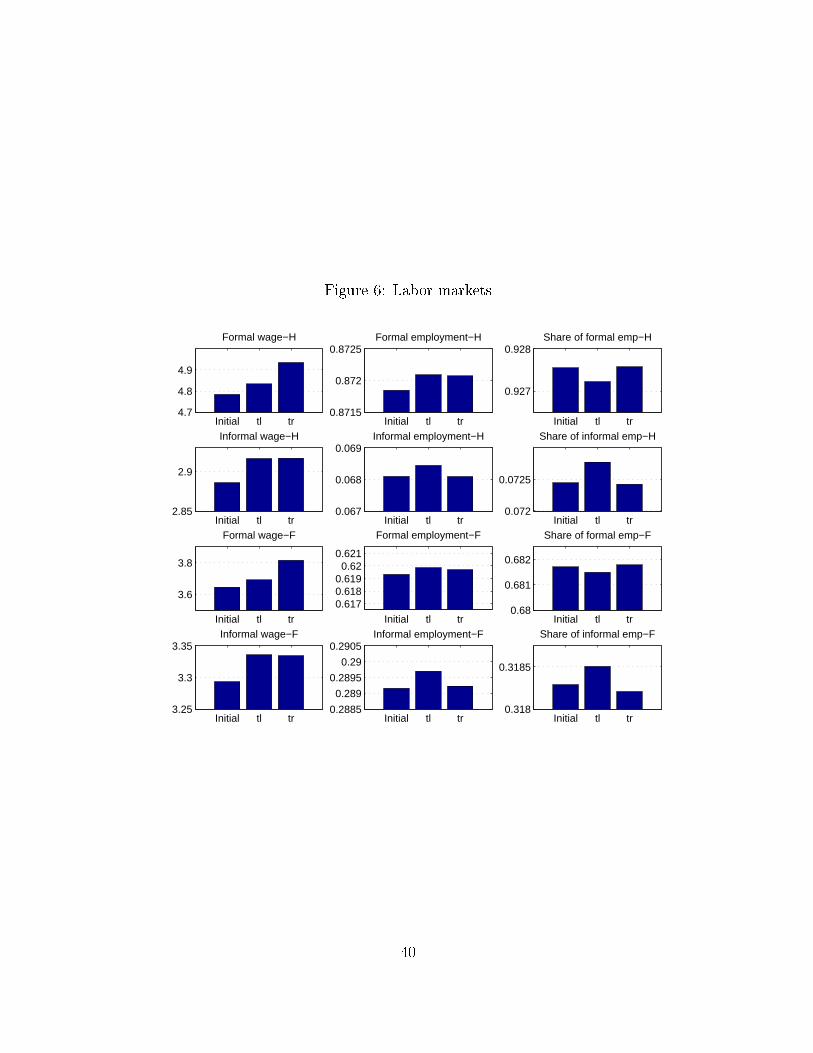
Figure 6: Labor markets

Initial tl tr4.7

4.8

4.9

Formal wage−H

Initial tl tr0.8715

0.872

0.8725Formal employment−H

Initial tl tr

0.927

0.928Share of formal emp−H

Initial tl tr2.85

2.9

Informal wage−H

Initial tl tr0.067

0.068

0.069Informal employment−H

Initial tl tr0.072

0.0725

Share of informal emp−H

Initial tl tr

3.6

3.8

Formal wage−F

Initial tl tr

0.6170.6180.619

0.620.621

Formal employment−F

Initial tl tr0.68

0.681

0.682

Share of formal emp−F

Initial tl tr3.25

3.3

3.35Informal wage−F

Initial tl tr0.2885

0.289

0.2895

0.29

0.2905Informal employment−F

Initial tl tr0.318

0.3185

Share of informal emp−F

40

Figure 7: Unemployment

Initial tl tr

0.0594

0.0596

0.0598

0.06

Unemployment−H

Initial tl tr1.36

1.365

1.37

1.375

1.38

1.385

Formal search effort−H

Initial tl tr1.01

1.015

1.02

1.025

1.03

1.035

1.04Informal search effort−H

Initial tl tr0.09

0.0905

0.091

0.0915

0.092Unemployment−F

Initial tl tr1.25

1.255

1.26

1.265Formal search effort−F

Initial tl tr1.2

1.205

1.21

1.215

1.22Informal search effort−F

Note: H and F indicate respectively the Home country (i.e. the developed country) and the Foreigncountry (i.e. the emerging country).

41