Can FPGAs Beat GPUs in Accelerating

Next-Generation Deep Neural Networks?

Eriko Nurvitadhi1, Ganesh Venkatesh1, Jaewoong Sim1, Debbie Marr1, Randy Huang2, Jason Gee Hock Ong2, Yeong Tat Liew2,

Krishnan Srivatsan3, Duncan Moss3, Suchit Subhaschandra3, Guy Boudoukh4

1Accelerator Architecture Lab,

2Programmable Solutions Group,

3FPGA Product Team,

4Computer Vision Group

Intel Corporation

ABSTRACT Current-generation Deep Neural Networks (DNNs), such as AlexNet and VGG, rely heavily on dense floating-point matrix multiplication (GEMM), which maps well to GPUs (regular parallelism, high TFLOP/s). Because of this, GPUs are widely used for accelerating DNNs. Current FPGAs offer superior energy efficiency (Ops/Watt), but they do not offer the performance of today’s GPUs on DNNs. In this paper, we look at upcoming FPGA technology advances, the rapid pace of innovation in DNN algorithms, and consider whether future high-performance FPGAs will outperform GPUs for next-generation DNNs.

The upcoming Intel® 14-nm StratixTM 10 FPGAs will have thousands of hard floating-point units (DSPs) and on-chip RAMs (M20K memory blocks). They will also have high bandwidth memories (HBMs) and improved frequency (HyperFlex™ core architecture). This combination of features brings FPGA raw floating point performance within striking distance of GPUs. Meanwhile, DNNs are quickly evolving. For example, recent innovations that exploit sparsity (e.g., pruning) and compact data types (e.g., 1-2 bit) result in major leaps in algorithmic efficiency. However, these innovations introduce irregular parallelism on custom data types, which are difficult for GPUs to handle but would be a great fit for FPGA’s extreme customizability.

This paper evaluates a selection of emerging DNN algorithms on two generations of Intel FPGAs (ArriaTM 10, StratixTM 10) against the latest highest performance Titan X Pascal GPU. We created a customizable DNN accelerator template for FPGAs and used it in our evaluations. First, we study various GEMM operations for next-generation DNNs. Our results show that Stratix 10 FPGA is 10%, 50%, and 5.4x better in performance (TOP/sec) than Titan X Pascal GPU on GEMM operations for pruned, Int6, and binarized DNNs, respectively. Then, we present a detailed case study on accelerating Ternary ResNet which relies on sparse GEMM on 2-bit weights (i.e., weights constrained to 0,+1,-1) and full-precision neurons. The Ternary ResNet accuracy is within ~1% of the full-precision ResNet which won the 2015 ImageNet competition. On Ternary-ResNet, the Stratix 10 FPGA can deliver 60% better performance over Titan X Pascal GPU, while being 2.3x better in

performance/watt. Our results indicate that FPGAs may become the platform of choice for accelerating next-generation DNNs.

Keywords Deep Learning, Accelerator, Intel Stratix 10 FPGA, GPU.

1. INTRODUCTION The exponential growth of digital data such as images,

videos, and speech, from myriad sources (e.g., social media, internet-of-things) is driving the need for analytics to extract knowledge from the data. Data analytics often rely on machine learning (ML) algorithms. Among ML algorithms, deep convolutional neural networks (DNNs) offer state-of-the-art accuracies for important image classification tasks, and therefore are becoming widely adopted.

Mainstream current-generation DNNs (e.g., AlexNet, VGG) rely heavily on dense matrix multiplication operations (GEMM) on 32-bit floating-point data (FP32). Such operations are well-suited for GPUs, which are known to do well on regular parallelism and are equipped with many floating-point compute units and high-bandwidth on-chip and off-chip memories. As such, recent GPUs are becoming more widely used for accelerating DNNs, since they can offer high performance (i.e., multi-TFLOP/s) for mainstream DNNs.

While FPGAs have provided superior energy efficiency (Performance/Watt) than GPUs for DNNs, they have not been known for offering top performance. However, FPGA technologies are advancing rapidly. The upcoming Intel Stratix 10 FPGA [17] will offer more than 5000 hardened floating-point units (DSPs), over 28MB of on-chip RAMs (M20Ks), integration with high-bandwidth memories (up to 4x250GB/s/stack or 1TB/s), and improved frequency from the new HyperFlex technology, thereby leading to a peak 9.2 TFLOP/s in FP32 throughput. In comparison, the latest Nvidia Titan X Pascal GPU offers 11 TFLOPs in FP32 throughput. This means that FPGA performance may be just within striking distance.

Moreover, DNN algorithms are evolving rapidly. Recent developments point toward next-generation DNNs that exploit network sparsity [4,5,6] and use extremely compact data types (e.g., 1bit, 2bit) [1,2,3,4,5]. These emerging DNNs offer orders of magnitude algorithmic efficiency improvement over “classic” DNNs that rely on dense GEMM on FP32 data type, but they introduce irregular parallelism and custom data types, which are difficult for GPUs to handle. In contrast, FPGAs are designed for extreme customizability. FPGAs shine on irregular parallelism and custom data types. An inflection point may be near!

Permission to make digital or hard copies of all or part of this work for personal or classroom use is granted without fee provided that copies are not made or distributed for profit or commercial advantage and that copies bear this notice and the full citation on the first page. Copyrights for components of this work owned by others than ACM must be honored. Abstracting with credit is permitted. To copy otherwise, or republish, to post on servers or to redistribute to lists, requires prior specific permission and/or a fee. Request permissions from Permissions@acm.org. FPGA’17, February 22-24, 2017, Monterey, CA, USA. © 2017 ACM. ISBN 978-1-4503-4354-1/17/02…$15.00.

DOI: http://dx.doi.org/10.1145/3020078.3021740

The key question is: For next-generation DNNs, can FPGAs beat GPUs in performance? This paper is the first to shed light on the answer by offering the following contributions:

First, we survey key trends in next-generation DNNs that exploit sparsity and compact data types. We cover pruned sparse networks [6], low N-bit networks [6,7], 1-bit binarized networks [1,2,3], and 2-bit sparse ternary networks [4,5].

Second, we develop a customizable DNN hardware accelerator template for FPGA that can support various next-generation DNNs. The template offers first-class hardware support for exploiting sparse computation and custom data types. It can be customized to produce optimized hardware instances for FPGA for a user-given variant of DNN.

Third, using the template, we evaluate various key matrix multiplication operations for next-generation DNNs. Our evaluation is done on the current- and next-generation of FPGAs (Arria 10, Stratix 10) and the latest high-performance Titan X Pascal GPU. We show that Stratix 10 FPGA is able to offer 10%, 50%, and 5.4x better in performance (TOP/sec) than Titan X Pascal GPU on GEMM operations for pruned, Int6, and binarized DNNs, respectively. We also show that both Arria 10 and Stratix 10 FPGAs offer compelling energy efficiency (TOP/sec/watt) relative to Titan X GPU.

Lastly, we conduct a case study on Ternary ResNet [5], where the key operation is multiplication of two sparse matrices. One matrix has FP32 values, and the other has ternary 2-bit values (i.e., weights are constrained to 0,+1,-1). The accuracy of Ternary ResNet [5] is within ~1% of the best reported accuracy of the most recent 2015 ImageNet competition winner (i.e., full-precision ResNet). For Ternary ResNet, the Stratix 10 FPGA can deliver 60% better performance than Titan X Pascal GPU, while being 2.3x better in performance/watt.

The rest of the paper is organized as follows. Section 2 provides background on DNN, FPGA, and GPU trends. Section 3 discusses our customizable DNN hardware accelerator template, which we use to derive FPGA implementation instances to evaluate against the GPU. Section 4 compares various types of GEMMs for next-generation DNNs. Section 5 presents a case study on Ternary ResNet on FPGAs and GPUs. Section 6, 7, and 8 offers discussions, related work, and concluding remarks.

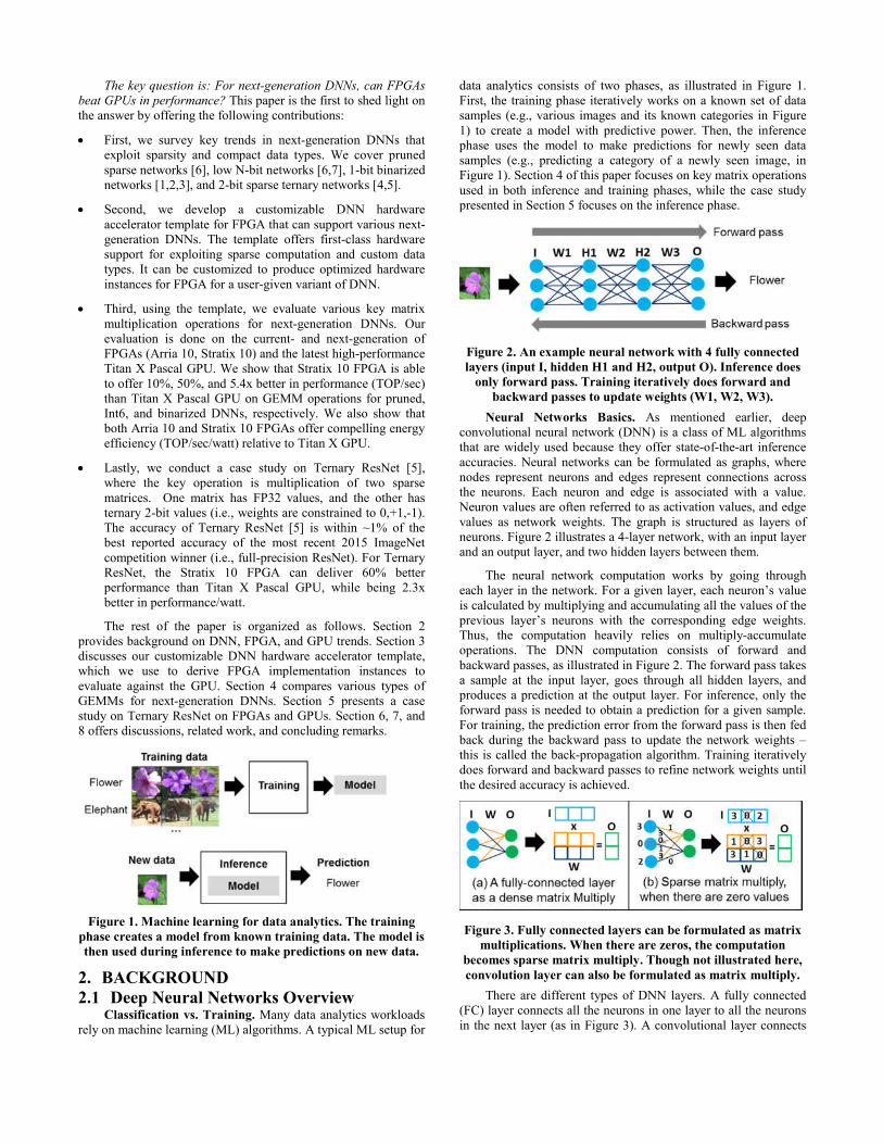
Figure 1. Machine learning for data analytics. The training phase creates a model from known training data. The model is then used during inference to make predictions on new data.

2. BACKGROUND 2.1 Deep Neural Networks Overview

Classification vs. Training. Many data analytics workloads rely on machine learning (ML) algorithms. A typical ML setup for

data analytics consists of two phases, as illustrated in Figure 1. First, the training phase iteratively works on a known set of data samples (e.g., various images and its known categories in Figure 1) to create a model with predictive power. Then, the inference phase uses the model to make predictions for newly seen data samples (e.g., predicting a category of a newly seen image, in Figure 1). Section 4 of this paper focuses on key matrix operations used in both inference and training phases, while the case study presented in Section 5 focuses on the inference phase.

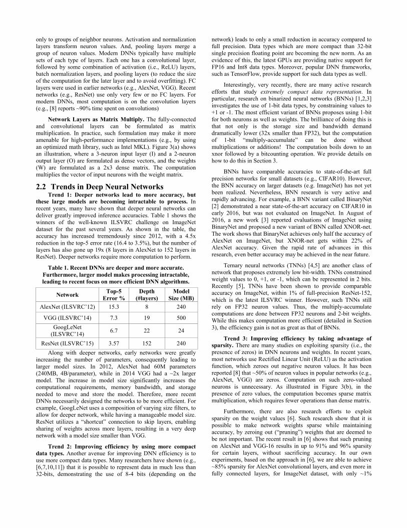
Figure 2. An example neural network with 4 fully connected layers (input I, hidden H1 and H2, output O). Inference does

only forward pass. Training iteratively does forward and backward passes to update weights (W1, W2, W3).

Neural Networks Basics. As mentioned earlier, deep convolutional neural network (DNN) is a class of ML algorithms that are widely used because they offer state-of-the-art inference accuracies. Neural networks can be formulated as graphs, where nodes represent neurons and edges represent connections across the neurons. Each neuron and edge is associated with a value. Neuron values are often referred to as activation values, and edge values as network weights. The graph is structured as layers of neurons. Figure 2 illustrates a 4-layer network, with an input layer and an output layer, and two hidden layers between them.

The neural network computation works by going through each layer in the network. For a given layer, each neuron’s value is calculated by multiplying and accumulating all the values of the previous layer’s neurons with the corresponding edge weights. Thus, the computation heavily relies on multiply-accumulate operations. The DNN computation consists of forward and backward passes, as illustrated in Figure 2. The forward pass takes a sample at the input layer, goes through all hidden layers, and produces a prediction at the output layer. For inference, only the forward pass is needed to obtain a prediction for a given sample. For training, the prediction error from the forward pass is then fed back during the backward pass to update the network weights – this is called the back-propagation algorithm. Training iteratively does forward and backward passes to refine network weights until the desired accuracy is achieved.

Figure 3. Fully connected layers can be formulated as matrix multiplications. When there are zeros, the computation

becomes sparse matrix multiply. Though not illustrated here, convolution layer can also be formulated as matrix multiply.

There are different types of DNN layers. A fully connected (FC) layer connects all the neurons in one layer to all the neurons in the next layer (as in Figure 3). A convolutional layer connects

only to groups of neighbor neurons. Activation and normalization layers transform neuron values. And, pooling layers merge a group of neuron values. Modern DNNs typically have multiple sets of each type of layers. Each one has a convolutional layer, followed by some combination of activation (i.e., ReLU) layers, batch normalization layers, and pooling layers (to reduce the size of the computation for the later layer and to avoid overfitting). FC layers were used in earlier networks (e.g., AlexNet, VGG). Recent networks (e.g., ResNet) use only very few or no FC layers. For modern DNNs, most computation is on the convolution layers (e.g., [8] reports ~90% time spent on convolutions)

Network Layers as Matrix Multiply. The fully-connected and convolutional layers can be formulated as matrix multiplication. In practice, such formulation may make it more amenable for high-performance implementations (e.g., by using an optimized math library, such as Intel MKL). Figure 3(a) shows an illustration, where a 3-neuron input layer (I) and a 2-neuron output layer (O) are formulated as dense vectors, and the weights (W) are formulated as a 2x3 dense matrix. The computation multiplies the vector of input neurons with the weight matrix.

2.2 Trends in Deep Neural Networks Trend 1: Deeper networks lead to more accuracy, but

these large models are becoming intractable to process. In recent years, many have shown that deeper neural networks can deliver greatly improved inference accuracies. Table 1 shows the winners of the well-known ILSVRC challenge on ImageNet dataset for the past several years. As shown in the table, the accuracy has increased tremendously since 2012, with a 4.5x reduction in the top-5 error rate (16.4 to 3.5%), but the number of layers has also gone up 19x (8 layers in AlexNet to 152 layers in ResNet). Deeper networks require more computation to perform.

Table 1. Recent DNNs are deeper and more accurate. Furthermore, larger model makes processing intractable, leading to recent focus on more efficient DNN algorithms.

Network Top-5

Error % Depth

(#layers) Model

Size (MB)

AlexNet (ILSVRC’12) 15.3 8 240

VGG (ILSVRC’14) 7.3 19 500

GoogLeNet (ILSVRC’14)

6.7 22 24

ResNet (ILSVRC’15) 3.57 152 240

Along with deeper networks, early networks were greatly increasing the number of parameters, consequently leading to larger model sizes. In 2012, AlexNet had 60M parameters (240MB, 4B/parameter), while in 2014 VGG had a ~2x larger model. The increase in model size significantly increases the computational requirements, memory bandwidth, and storage needed to move and store the model. Therefore, more recent DNNs necessarily designed the networks to be more efficient. For example, GoogLeNet uses a composition of varying size filters, to allow for deeper network, while having a manageable model size. ResNet utilizes a “shortcut” connection to skip layers, enabling sharing of weights across more layers, resulting in a very deep network with a model size smaller than VGG.

Trend 2: Improving efficiency by using more compact data types. Another avenue for improving DNN efficiency is to use more compact data types. Many researchers have shown (e.g., [6,7,10,11]) that it is possible to represent data in much less than 32-bits, demonstrating the use of 8-4 bits (depending on the

network) leads to only a small reduction in accuracy compared to full precision. Data types which are more compact than 32-bit single precision floating point are becoming the new norm. As an evidence of this, the latest GPUs are providing native support for FP16 and Int8 data types. Moreover, popular DNN frameworks, such as TensorFlow, provide support for such data types as well.

Interestingly, very recently, there are many active research efforts that study extremely compact data representation. In particular, research on binarized neural networks (BNNs) [1,2,3] investigates the use of 1-bit data types, by constraining values to +1 or -1. The most efficient variant of BNNs proposes using 1-bit for both neurons as well as weights. The brilliance of doing this is that not only is the storage size and bandwidth demand dramatically lower (32x smaller than FP32), but the computation of 1-bit “multiply-accumulate” can be done without multiplications or additions! The computation boils down to an xnor followed by a bitcounting operation. We provide details on how to do this in Section 3.

BNNs have comparable accuracies to state-of-the-art full precision networks for small datasets (e.g., CIFAR10). However, the BNN accuracy on larger datasets (e.g. ImageNet) has not yet been realized. Nevertheless, BNN research is very active and rapidly advancing. For example, a BNN variant called BinaryNet [2] demonstrated a near state-of-the-art accuracy on CIFAR10 in early 2016, but was not evaluated on ImageNet. In August of 2016, a new work [3] reported evaluations of ImageNet using BinaryNet and proposed a new variant of BNN called XNOR-net. The work shows that BinaryNet achieves only half the accuracy of AlexNet on ImageNet, but XNOR-net gets within 22% of AlexNet accuracy. Given the rapid rate of advances in this research, even better accuracy may be achieved in the near future.

Ternary neural networks (TNNs) [4,5] are another class of network that proposes extremely low bit-width. TNNs constrained weight values to 0, +1, or -1, which can be represented in 2 bits. Recently [5], TNNs have been shown to provide comparable accuracy on ImageNet, within 1% of full-precision ResNet-152, which is the latest ILSVRC winner. However, such TNNs still rely on FP32 neuron values. Thus, the multiply-accumulate computations are done between FP32 neurons and 2-bit weights. While this makes computation more efficient (detailed in Section 3), the efficiency gain is not as great as that of BNNs.

Trend 3: Improving efficiency by taking advantage of sparsity. There are many studies on exploiting sparsity (i.e., the presence of zeros) in DNN neurons and weights. In recent years, most networks use Rectified Linear Unit (ReLU) as the activation function, which zeroes out negative neuron values. It has been reported [8] that ~50% of neuron values in popular networks (e.g., AlexNet, VGG) are zeros. Computation on such zero-valued neurons is unnecessary. As illustrated in Figure 3(b), in the presence of zero values, the computation becomes sparse matrix multiplication, which requires fewer operations than dense matrix.

Furthermore, there are also research efforts to exploit sparsity on the weight values [6]. Such research show that it is possible to make network weights sparse while maintaining accuracy, by zeroing out (“pruning”) weights that are deemed to be not important. The recent result in [6] shows that such pruning on AlexNet and VGG-16 results in up to 91% and 96% sparsity for certain layers, without sacrificing accuracy. In our own experiments, based on the approach in [6], we are able to achieve ~85% sparsity for AlexNet convolutional layers, and even more in fully connected layers, for ImageNet dataset, with only ~1%

degradation in accuracy. We were also able to prune GoogleNet with only ~0.2% drop in accuracy, while achieving ~65% sparsity for all convolution layers, except for the first layer.

Another method to sparsify weights is by ternarization. As mentioned earlier, TNNs constrain weights to 0, +1, or -1. Thus, it introduces many zeros to the weights. A Ternarized ResNet that delivers comparable accuracy to full-precision ResNet introduces ~50% sparsity to the weights.

Other Trends. DNN research is rapidly evolving and there are trends not covered in this paper. We offer discussions on these in Section 6. Nevertheless, we believe that sparsity exploitation and the use of extremely compact data types are two major trends likely to become the norm in the next-generation DNNs. Therefore, we focus on these in the remainder of the paper.

2.3 GPU vs. FPGA Trends GPUs are known to do well on data parallel computation that

exhibits regular parallelism and demands high floating point compute throughput. Across generations, GPUs offer increased FLOP/s, by incorporating more floating-point units, on-chip RAMs, and higher memory bandwidth. For example, the latest Titan X Pascal offers peak 11 TFLOP/s of 32-bit floating-point throughput, a noticeable improvement from the previous generation Titan X Maxwell that offered 7 TFLOP/s peak throughput. However, GPUs can face challenges from issues, such as divergence, for computation that exhibits irregular parallelism. Further, GPUs support only a fixed set of native data types. So, other custom-defined data types may not be handled efficiently. These challenges may lead to underutilization of hardware resources and unsatisfactory achieved performance.

Meanwhile, FPGAs have advanced significantly in recent years. There are several FPGA trends to consider. First, there are much more on-chip RAMs on next-generation FPGAs. For example, Stratix 10 [17] offers up to ~28 MBs worth of on-chip RAMs (M20Ks). Second, frequency can improve dramatically, enabled by technologies such as HyperFlex. Third, there are many more hard DSPs available. Fourth, off-chip bandwidth will also increase, with the integration of HBM memory technologies. Fifth, these next-generation FPGAs use more advanced process technology (e.g., Stratix 10 uses 14nm Intel technology). Overall, it is expected that Intel Stratix 10 can offer up to 9.2 TFLOP/s of 32bit floating-point performance. This brings FPGAs closer in raw performance to state-of-the-art GPUs. Unlike GPUs, the FPGA fabric architecture was made with extreme customizability in mind, even down to bit-levels. Hence, FPGAs have the opportunity to do increasingly well on the next-generation DNNs as they become more irregular and use custom data types.

In addition, the software ecosystem for FPGAs is advancing as well. High-level FPGA programming tools (e.g., Altera OpenCL SDK) are now commercially available. They allow programming FPGAs at a higher level of abstraction than RTL (e.g., Verilog). These tools make FPGAs more accessible to developers who are not hardware experts. FPGAs are integrating into mainstream compute systems, e.g., alongside a server CPU in an upcoming Intel Xeon®+FPGA offering [12], inside a network card, or as a “GPU form factor” PCIe card. These trends can speed up FPGA adoption into the mainstream systems. Indeed, there are ongoing efforts from leading technology companies to incorporate FPGAs into datacenters (e.g., [12,13]).

3. CUSTOMIZABLE HARDWARE ARCHITECTURE TEMPLATE FOR DNNS

We have developed customizable hardware architecture “template” for DNNs, which takes into account the emerging DNN trends mentioned in Section 2 (i.e., sparsity, compact data types). The template can be configured to derive hardware instances (i.e., RTL implementation) for a given user-specified DNN variant. Such instances can then be mapped to FPGA (or ASIC). We use this template to facilitate our evaluations of next-generation DNNs on FPGAs and to compare them against GPUs, which we will discuss in the next two sections. Meanwhile, we describe our customizable DNN hardware template in this section.

Figure 4. Customizable hardware architecture template for DNNs. (a) shows top-level design. (b) and (c) show variants of GEMM unit supported by our template. (d) and (f) show PE

designs for handling dense and sparse data. (e) shows optimization for binarized GEMM, where multiply-

accumulate operation is done using xnor and bitcounting.

3.1 Overview The top-level design of our template is shown in Figure 4(a).

The design consists of Memory and On-chip data management units (MDM, ODM), GEMM Unit to compute convolutional and fully connected layers, and Misc Layers Unit (MLU) to compute the other DNN layer types (ReLU, Batch Norm, Pool).

The design works as follows. First, weights and input neurons are loaded into on-chip buffers in ODM from memory. The convolution and fully-connected layers are computed by dynamically flattening the weights and input feature maps (neurons) onto blocked matrix operations, as in [10]. The GEMM Unit performs such matrix operations and outputs the result to MLU, which then performs the ReLu/BatchNorm/Pooling layers, as dictated by the desired DNN configuration. The output goes into the on-chip buffer in ODM, to be read by the next convolution/FC layer. If there is not enough buffer in ODM, the output is spilled out to memory by MDM.

The GEMM Unit consists of multiple processing elements (PEs). The GEMM Unit is customizable to use systolic-based [14] or broadcast-based [15] architecture across PEs, as shown in Figures 4(b) and 4(c). PE is customizable to be able to perform one or more multiply-accumulate operations.

In overall, the template is customizable to use various GEMM and PE architectures (systolic/broadcast; sparse/dense) and data types (1bit/2bit/Nbit/FP), as well as the typical sizing parameters (e.g., number of PEs, GEMM units, buffer sizes, etc.).

3.2 Support for Emerging DNNs Our architecture template incorporates features to exploit

sparsity and to handle compact data types, which are needed by emerging DNNs. We describe these features below.

3.2.1 Support for N-bit data type FPGAs have been known to be extremely flexible to handle

various data types. Many prior DNN works (e.g., [6,7,10,11]) have shown promising results implementing customized N-bit data. Our architecture template can also support customization to N-bit data. PEs can be customized to handle varying width of dot product calculations based on data type width. Accordingly, the data management units (ODM, MDM) can be customized to handle packing/unpacking of the desired N-bit data types.

3.2.2 Support for Sparse Pruned DNNs There are many existing studies on processing sparse

matrices (e.g., in HPC applications). However, such studies typically use matrices that are extremely sparse (i.e., 1% or less non-zeros). We observe that the sparsity in DNNs is not as extreme (i.e., ~5-50% non-zeros). Therefore, instead of utilizing a sparse matrix format (e.g., CSR), we opted to use a dense format, but dynamically checked/tracked zeros and skipped zero computation (i.e., similar to the approach from [8]). Specifically, prior to feeding data to GEMM Unit, on-chip data manager checks for zero values and includes metadata (index or bitvector) to identify the locations of the zeros in the block of data providing to the GEMM unit. Each processing element (PE) inside the GEMM unit will read a set of matrix elements along with the metadata. It will then schedule computation based on information in the metadata. Those zero elements are not scheduled onto the multiply-accumulate compute units inside the PE, therefore reducing number of cycles needed to complete the matrix operations and improving overall performance. The design of the PE to support sparsity is shown in Figure 4(f). In contrast, the PE design for regular dense computation is shown in Figure 4(d).

Figure 5. Binarized Matrix Multiplication. By representing -1 as 0, standard multiply and add operations (a) can be replaced

by xnor and bit counting operations (b), where bit counting can be done using a lookup table (c).

3.2.3 Support for Binarized DNNs In binarized DNNs (BNNs), both weight and neuron values

are constrained to +1 or -1. Therefore, the key operation in BNNs is 1-bit matrix multiplication. Figure 5(a) shows an example of a 1-bit matrix multiply. To improve computation efficiency -1 can be represented as zeros, and computation can be done using an xnor followed by a bit counting operation (as in Figure 5(b)). The bit counting itself can further be implemented using a lookup table, as shown in Figure 5(c). Our DNN architecture template provides a customization option for a PE that performs N-bit dot products using the aforesaid approach, as depicted in Figure 4(e).

3.2.4 Support for Ternarized DNNs Lastly, the support for Ternarized DNNs (TNNs) in our

architecture is as follows. In TNNs, weights are constrained to 0, +1, or -1, but neurons are still using N-bit precision. In this case, we represent ternary weights using 2 bits, with 1 bit indicating whether the value is 0 and another bit indicating whether the value is +1 or -1 (as in BNNs). The PE uses the 1-bit zero indicator in the same way as the metadata bits used to exploit sparsity in Section 3.2.2. As such, whenever there is an operation against a zero weight, the operation will be skipped and not be scheduled onto the PE’s compute unit(s). If the weight is either +1 or -1, instead of performing multiplication against N-bit precision neuron values, we simplify the computation by negating the sign of the neuron value (i.e., a sign bit flip if neuron is floating-point, or negation if it is fixed point). As such, PE for ternary computation does not require a multiplication unit.

4. EVALUATION OF MATRIX MULTIPLY FOR NEXT-GENERATION DNNS

Matrix multiplication is a key operation in DNNs. It is important to have a thorough understanding of the achievable peak performance of this key operation on the platforms studied. For this reason, we evaluate matrix multiplication on a variety of matrix and data types. We selected dense and sparse matrices, 32-bit floating point data types vs. narrow bit-width data types, and even an extremely compact binarized 1-bit data type.

Table 2. FPGAs and GPU under study. Based on [16,17,18]

Type Arria 10 1150

FPGA Stratix 10 2800

FPGA TitanX Pascal

GPU Peak FP32 TFLOPs

1.36 9.2 11

On-chip RAMs

6.6 MB (M20Ks)

28.6 MB (M20Ks)

13.5 MB (RF, SM, L2)

Memory BW Assume same

as Titan X Assume same as

Titan X 480 GB/s

4.1 Methodology Since we would like to understand the top possible

performance achievable by FPGAs and GPUs for the types of matrix multiplications under study, we allow freely choosing matrix sizes that provide the best performance for the target platform. This ended up being in the range of dimensions of 2K-4K. We also chose amenable batch sizes (i.e., number of independent matrix multiplications), since batching is a common practice when running DNNs on GPUs to maximize throughput.

The specific FPGAs and GPU studied are shown in Table 2. We include two generations of FPGAs (Arria 10 and Stratix 10) and compare them with the Titan X Pascal GPU, the latest and highest performance GPU available for purchase at this paper’s submission deadline (September of 2016).

To make a fair FPGA comparison to the GPU, we decided to allow the FPGA to have the same memory capacity and bandwidth as the GPU. Although readily-available FPGA cards have less capable memory system than the GPU card, integrated HBM stacks in the upcoming Stratix 10 will allow FPGA packages and cards to have the equivalent memory bandwidth and capacity as the GPU cards. We want to evaluate the potential fundamental advantages of FPGA vs. GPU rather than penalizing our FPGA study with memory limitations that can be addressed with packaging and card-level solutions.

For our FPGA evaluation, we derived RTL instances from our DNN hardware template, with customizations selected to optimize for the matrix operations under study. Then, we use Altera QuartusTM software, EPE tool [19], analytical modeling, and simulations to estimate performance and power. For Stratix 10, which has been announced, but not yet available, we use Quartus Early Beta release. Note that its quality is not necessarily reflective of future more mature releases of Quartus for Stratix 10.

For our GPU evaluation, we conduct real system measurements on the Nvidia Titan X Pascal card. We use nvprof to collect performance and power numbers.

4.2 “Classic” DNNs Current mainstream (i.e., “classic”) DNNs, such as AlexNet,

VGG, Googlenet, ResNet, etc., typically rely on dense matrix multiplication on single-precision floating point numbers (FP32).

Figure 6. Matrix multiplication results for “Classic” DNNs. It

operates on dense matrices with FP32 data type

For GPU, we measured the FP32 dense matrix multiplication performance using the cuBLAS library in the Nvidia CUDA Toolkit 8.0 RC. Most of the instructions in the cuBLAS SGEMM implementation are FMAs, leading to high compute efficiency. The peak theoretical performance of Titan X Pascal is 11 TFLOPs, and we achieved 10.88 TFLOPs with the cuBLAS matrix multiplication library call.

FP32 dense matrix multiplication is a sweet spot for GPUs, not FPGAs, so we did not create an optimized FPGA implementation for this. We present comparison of peak numbers based on the FPGA and GPU datasheets instead (in Figure 6).

As Figure 6(a) shows, Stratix 10 with its far greater number of DSPs will offer much improved FP32 performance compared to the Arria 10, bringing the Stratix 10 within striking distance to Titan X performance. However, the peak FP32 TOP/s still lags behind the GPU. It could be possible for FPGAs to win in performance/Watt. Figure 6(b) shows that the Stratix 10 can be up to ~40% better than Titan X if we assume the FPGA peak TOP/s.

4.3 Sparse (Pruned) DNNs As described in Section 2, next-generation DNNs are likely

to operate on sparse matrices. Pruning [6] is a recent, popular

technique to make DNN weights sparse without little or no loss in accuracy. For our study, we replicated the pruning results for AlexNet from [6] using our in-house software reference. We also ran further experiments to fine-tune (e.g., pruning threshold, number of re-training iterations) and optimize our results. We are able to achieve on average ~85% sparsity in the convolution layers of AlexNet with less than a 1% degradation in accuracy (fully connected layers are even more sparse). Hence, our evaluation uses matrices with 85% sparsity (i.e., 15% non-zeros).

4.3.1 Sparse Matrix Multiply on GPU Evaluating sparse matrix multiply for pruned DNNs can be

challenging for GPUs. Modern GPU architectures employ what is known as a single-instruction multiple-thread (SIMT) execution model, in which multiple threads execute the same sequence of instructions, on different data, in a lock step fashion. As such, although a few threads may skip zero computation, the corresponding SIMT lanes simply remain idle while the threads on the other SIMT lanes perform non-zero computation. In addition, checking for zeros in the matrices adds extra instructions to the execution kernel, which reduces compute efficiency.

Another approach is to use sparse linear algebra libraries for zero-skipping. However, existing GPU libraries such as cuSPARSE are targeted for traditional sparse matrix operations that perform on extremely sparse matrices with less than 1% of zeros (e.g., well-known in the High-Performance Computing domain). Also, for sparse matrix multiplication, the input matrices need to be converted to one of the standard sparse matrix formats such as compressed sparse row (CSR) or compressed sparse column (CSC). Since the matrices in DNNs are not extremely sparse (i.e., ~5%-50% sparsity), using these sparse libraries leads to large overhead.

To address this problem, we wrote our own sparse matrix multiply implementation. Our implementation uses dense matrix format, but it checks and skips zeros dynamically in a similar way as our FPGA implementation. Our implementation is a modification on top of an optimized open-source MAGMA [29] dense matrix multiply library. While we would have liked to implement our algorithm on top of cuBLAS, the code for cuBLAS is not open-source. The MAGMA library is one of the most optimized open-source GPU libraries that we could find.

Figure 7. GPU performance on sparse (zero-skipping) GEMM versus dense GEMM for various sparsity levels. Zero-skipping

sparse GEMM performs worse than normal dense GEMM.

Figure 7 shows the comparison between the baseline SGEMM (without zero-skipping) and SGEMM with zero-skipping for varying sparsity levels. As explained before, dynamically checking zero values degrades performance as it needs to execute more non-useful instructions, without increasing SIMT utilization. Across the different sparsity percentages, zero-skipping kernel performs worse than without zero-skipping. Hence, for comparison against FPGA, we use GPU performance on dense matrix multiplication. This is because the GPU performance is far better on dense matrix, computing all the

0

5000

10000

0 25 50 75

GFL

OP

s

Sparsity (%)

Baseline Zero-Skipping

multiplications, including the zeros. Specifically, we use the cuBLAS library in the Nvidia CUDA Toolkit 8.0 RC.

Figure 8. Matrix multiplication results for DNNs with pruning. It operates on sparse matrices with FP32 data type. We use 85% sparsity, based on pruned AlexNet experiments.

For GPU, we report achieved performance on FP32 dense matrix multiply, since we found that sparse matrix

multiplication lead to GPU performance degradation.

4.3.2 Sparse Matrix Multiply on FPGA For FPGA, we use the design described in Section 3.2.2.

Since on FPGA we can detect and skip zero computation in a fine grained manner, at 85% sparsity we observe ~4x speedups in cycle count, as our GEMM Unit is able to skip many zeros.

For Stratix 10, we made conservative, moderate, and aggressive performance projections. The conservative estimate is based on mapping and scaling up our GEMM implementation for Arria 10 directly to Stratix 10 without doing any optimization for HyperFlex to achieve higher frequency. Hence, the conservative estimate uses 300MHz frequency, matching the Arria 10 design. The moderate and aggressive projections anticipate frequency boosts from HyperFlex to 500MHz and 700MHz, respectively.

4.3.3 FPGA vs. GPU The performance and performance/watt for FPGAs and GPU

under study is shown in Figure 8. As shown in Figure 8(a), even the conservative 300 MHz estimate for Stratix 10 is only ~34% worse in performance than GPU. The moderate estimate using 500 MHz brings Stratix 10 performance to ~10% better than GPU, and the aggressive estimate improves it even further.

In terms of performance/watt, Figure 8(b) shows that FPGAs offer more compelling results than GPU across the board. Arria 10 offers 16% better performance/watt over GPU, with Stratix 10 offering even further improvements.

Figure 9. Matrix multiplication results for DNNs with compact data types. It operates on dense matrices. We use 6-bit (Int6) data type for FPGA. For GPU, which does not have

native support for Int6, we use theoretical peak Int8 GPU performance for comparison.

4.4 Compact Narrow-Bitwidth DNNs As described in Section 2, there is significant prior work in

quantizing data to reduce computation requirements and bit-widths to values smaller than 32-bit floating point. While 8-bit or larger data types were used in the past DNN proposals, there are trends towards even smaller sub-8-bit data types [6,7]. Here, we evaluate dense matrix multiplication using the Int6 data type.

We use FPGA implementation based on systolic GEMM (shown in Figure 4(b)) that is well optimized for frequency. It can achieve 440MHz for Arria 10 and 920MHz in Stratix 10. For GPU, we use theoretical peak Int8 performance for Titan X, since GPU does not have native support for Int6 computations.

Our evaluation results are shown in Figure 9. As Figure 9(a) shows, Stratix 10 Int6 performance is more than 50% better than the Titan X theoretical peak Int8 performance (Titan X Int6 performance is expected to not be better than Int8). As Figure 9(b) shows, performance/watt of FPGA is either comparable (Arria 10) or more than 2x better (Stratix 10) than Titan X GPU.

4.5 Binarized DNNs Recent “binarized” DNNs have proposed using extremely

compact 1bit data types. As detailed earlier, 1bit matrix multiplications in binarized DNNs can be done more optimally using xnor and bitcounting operations.

For GPU evaluation, we use a binary matrix multiply kernel (xnor_gemm) from BinaryNet [2], which is based on the blocked version of matrix multiply in the CUDA Programming Guide. In the xnor_gemm implementation, instead of performing FMA operations for matrix multiply, each CUDA thread performs xnor and population count operations to compute one element of the resulting matrix. The population count operation is supported in Nvidia GPUs via __popc() (for 32-bit) and __popcll() (for 64-bit) intrinsic functions. When these intrinsics are used in the CUDA kernel, the CUDA compiler maps __popc() to a single instruction and __popcll() to a few instructions.

On Titan X Pascal, 32 32-bit population count operations can be issued every cycle per Streaming Multiprocessor (SM), which leads to 1024 “binary ops” per cycle per SM. As Titan X can issue up to 128 FP32 FMA instructions every cycle per SM, the peak throughput of “binary ops” over FP32 operations is 4x. In our Titan X Pascal, we achieve 45.6 TOPs for binary GEMM performance.

For FPGA, we use systolic array GEMM unit with the PE for binarized DNNs, which we described earlier in Section 3.2.3. Our PE is configured to do 256-wide binary dot product operations. We synthesized our implementation to Arria 10 and Stratix 10. For validation, we also deployed and ran the design on an Arria 10 development system.

Figure 10. Matrix multiplication results for binarized DNNs. It operates on dense matrices with 1bit data types. Multiply

and add operations are replaced with xnor and bitcount.

Our evaluation results are shown in Figure 10. Stratix 10 can deliver 3x (conservative) to 12x (aggressive) better performance than achieved performance on Titan X GPU, and 70% (conservative) and over 6x (aggressive) than theoretical performance of Titan X. Meanwhile, Arria 10 can deliver 25% better performance than achieved Titan X GPU performance. In terms of performance/watt, the Arria 10 and Stratix 10 can deliver 3x to over 10x better energy efficiency relative to Titan X.

5. TERNARY RESNET CASE STUDY In the previous section, we evaluated key operations in

various emerging DNNs. In this section, we zoom in on a specific DNN. In particular, we report a case study on accelerating Ternary version of the state-of-the-art ResNet [5].

5.1 Ternary ResNet Overview Ternary DNNs (i.e., Ternary Weight Networks) [4,5] have

recently proposed constraining neural network weights to +1, 0, or -1, allowing for weights to be represented with just 2 bits, while simultaneously introducing more sparsity to these weights. Neurons are still represented using full precision (FP32). The reported ImageNet accuracy results on Ternary DNNs have been very compelling. The earlier paper [4] in May 2016 reported only 1.8% top-5 accuracy degradation on Ternary ResNet-18 relative to full precision ResNet-18 (i.e., 86.2% Ternary vs. 88% full precision accuracies). The very recent work [5] in September 2016 reports only 0.64% accuracy degradation for ResNet-152 (i.e., 93.2% ternary vs. 93.84% full precision). This work also reports accuracy for ternary ResNet-50, which is within 1% accuracy of full precision ResNet-50. We focus on ResNet-50 here, since its accuracy is close to ResNet-152 (within ~1.2%), but requires much less computation.

Figure 11. Sparsity of Ternary ResNet-50. The x-axis shows the different layers of ResNet-50. The y-axis shows

percentages of zeros for each layer. Sparsity results for the ternary weights and runtime neuron values are provided.

Figure 12. FPGA accelerator speedups from exploiting sparsity for each Ternary ResNet-50 layer. E.g., 1.5 means

that enabling sparse support to skip zeros leads to 1.5x faster run (in cycle count) over normal dense processing.

5.2 Software Reference and Sparsity Study Our software reference is based on the work in [5], which is

built on top of the Torch framework for ResNet [20]. We ran our

own experiments on ImageNet dataset with Ternary ResNet. Indeed, we were able to obtain accuracies mentioned earlier.

First, to understand the opportunity for sparsity exploitation, we collected average sparsity data for the resulting weights from training with Ternary ResNet-50. Since ResNet uses ReLU as the activation function, we also report runtime sparsity at the input neuron values. Figure 11 shows the results.

As Figure 11 shows, the sparsity varies layer by layer. On a weighted average across the layers, the weights are 51% sparse and the neurons are 60% sparse. This means, that in the upper bound, there can be 70-80% overall sparsity across both the weights and neurons. In an ideal case, if it is possible to avoid the 70-80% unnecessary zero computations with perfect efficiency, the upper bounds for speedups are 3.3x-5x. While this is promising, in practice the actual speedups depend on whether the compute platform can avoid these zero computations efficiently.

5.3 FPGA Evaluation We used the hardware template detailed in Section 3 and

considered several possible instances of RTL implementations for Ternary ResNet-50. In particular, we enabled customizations for ternary DNNs discussed in Section 3.2.4.

First, we customized for 2bit ternary data format, and replaced multiplication with a sign bit manipulation. Thus, our PE only contains a floating-point accumulator. Nevertheless, a single Stratix 10 DSP block contains an FP32 multiplier and an FP32 adder. Even though we are not using the multiplier, we still have to use an entire DSP for our accumulator, so we do not gain any DSP savings in this case. We do obtain ALM and M20K savings from having very compact 2-bit ternary data representation.

Second, we evaluated different configurations for zero skipping support. Generally, there is a tradeoff between the aggressiveness of our sparse data scheduler to skip zero computations and the FPGA resources needed and frequency. A more aggressive sparse scheduler can look further ahead to a larger set of weights and/or neurons, and identify and skip larger portions of zeros dynamically. However, it costs more resources and may impact frequency if it introduces data dependencies.

For this study, we chose a simper design more amenable to frequency optimizations. Specifically, we opted for a less aggressive but simpler sparse scheduler, at the expense of less opportunity to skip zero computations. Furthermore, instead of having the sparse scheduler skip zeros on both neurons and weights, we chose to skip only zero neurons, as they use wider 32-bit data type and sparser than the weights. Zero skipping only on neurons lets us use only one of the “Sparse Mgt” unit outside of the GEMM unit (i.e., inside “ODM” in Figure 4(a)) and to simplify “zero-skip scheduler” inside each PE. Based on ResNet-50 layer dimensions, we customize our DNN accelerator with GEMM units with 4x8 PEs and 8 FMA units/PE.

Figure 12 shows our simulation results. We get only ~2x reduction in cycle count from skipping zeros, even though as stated earlier the upper bounds for exploiting sparsity are 3.3x-5x speedups. More comprehensive design exploration is needed to find an optimal design point. We leave this for a future study.

Because we exploit sparsity less aggressively, we ended up with a simpler more regular design that is amenable to frequency optimizations. The design runs at 450 MHz, even without explicitly optimizing for HyperFlex yet. Due to time constraints, we are not yet able to fully optimize our design. We are also using

Quartus Early Beta release for Stratix 10. Even though this is the latest version available to us at present, it may or may not reflect the synthesis result of more mature future releases of Quartus for Stratix 10. Due to this, we made projections with conservative, moderate, and aggressive optimization targets. Our conservative estimate targets 450MHz, which we currently already achieved without explicit optimizations for HyperFlex. HyperFlex has been reported to enable much higher frequency (e.g., 896MHz in 400G Ethernet CRC assembly [22]), so we use 600MHz and 750MHz as our moderate and aggressive projections.

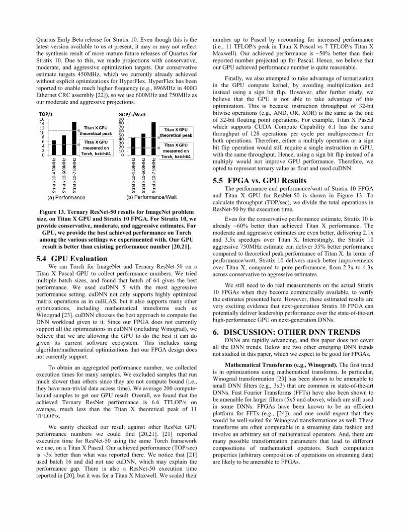
Figure 13. Ternary ResNet-50 results for ImageNet problem size, on Titan X GPU and Stratix 10 FPGA. For Stratix 10, we provide conservative, moderate, and aggressive estimates. For

GPU, we provide the best achieved performance on Torch among the various settings we experimented with. Our GPU result is better than existing performance number [20,21].

5.4 GPU Evaluation We ran Torch for ImageNet and Ternary ResNet-50 on a

Titan X Pascal GPU to collect performance numbers. We tried multiple batch sizes, and found that batch of 64 gives the best performance. We used cuDNN 5 with the most aggressive performance setting. cuDNN not only supports highly optimized matrix operations as in cuBLAS, but it also supports many other optimizations, including mathematical transforms such as Winograd [23]. cuDNN chooses the best approach to compute the DNN workload given to it. Since our FPGA does not currently support all the optimizations in cuDNN (including Winograd), we believe that we are allowing the GPU to do the best it can do given its current software ecosystem. This includes using algorithm/mathematical optimizations that our FPGA design does not currently support.

To obtain an aggregated performance number, we collected execution times for many samples. We excluded samples that run much slower than others since they are not compute bound (i.e., they have non-trivial data access time). We average 200 compute-bound samples to get our GPU result. Overall, we found that the achieved Ternary ResNet performance is 6.6 TFLOP/s on average, much less than the Titan X theoretical peak of 11 TFLOP/s.

We sanity checked our result against other ResNet GPU performance numbers we could find [20,21]. [21] reported execution time for ResNet-50 using the same Torch framework we use, on a Titan X Pascal. Our achieved performance (TOP/sec) is ~3x better than what was reported there. We notice that [21] used batch 16 and did not use cuDNN, which may explain the performance gap. There is also a ResNet-50 execution time reported in [20], but it was for a Titan X Maxwell. We scaled their

number up to Pascal by accounting for increased performance (i.e., 11 TFLOP/s peak in Titan X Pascal vs 7 TFLOP/s Titan X Maxwell). Our achieved performance is ~50% better than their reported number projected up for Pascal. Hence, we believe that our GPU achieved performance number is quite reasonable.

Finally, we also attempted to take advantage of ternarization in the GPU compute kernel, by avoiding multiplication and instead using a sign bit flip. However, after further study, we believe that the GPU is not able to take advantage of this optimization. This is because instruction throughput of 32-bit bitwise operations (e.g., AND, OR, XOR) is the same as the one of 32-bit floating point operations. For example, Titan X Pascal which supports CUDA Compute Capability 6.1 has the same throughput of 128 operations per cycle per multiprocessor for both operations. Therefore, either a multiply operation or a sign bit flip operation would still require a single instruction in GPU, with the same throughput. Hence, using a sign bit flip instead of a multiply would not improve GPU performance. Therefore, we opted to represent ternary value as float and used cuDNN.

5.5 FPGA vs. GPU Results The performance and performance/watt of Stratix 10 FPGA

and Titan X GPU for ResNet-50 is shown in Figure 13. To calculate throughput (TOP/sec), we divide the total operations in ResNet-50 by the execution time.

Even for the conservative performance estimate, Stratix 10 is already ~60% better than achieved Titan X performance. The moderate and aggressive estimates are even better, delivering 2.1x and 3.5x speedups over Titan X. Interestingly, the Stratix 10 aggressive 750MHz estimate can deliver 35% better performance compared to theoretical peak performance of Titan X. In terms of performance/watt, Stratix 10 delivers much better improvements over Titan X, compared to pure performance, from 2.3x to 4.3x across conservative to aggressive estimates.

We still need to do real measurements on the actual Stratix 10 FPGAs when they become commercially available, to verify the estimates presented here. However, these estimated results are very exciting evidence that next-generation Stratix 10 FPGA can potentially deliver leadership performance over the state-of-the-art high-performance GPU on next-generation DNNs.

6. DISCUSSION: OTHER DNN TRENDS DNNs are rapidly advancing, and this paper does not cover

all the DNN trends. Below are two other emerging DNN trends not studied in this paper, which we expect to be good for FPGAs.

Mathematical Transforms (e.g., Winograd). The first trend is in optimizations using mathematical transforms. In particular, Winograd transformation [23] has been shown to be amenable to small DNN filters (e.g., 3x3) that are common in state-of-the-art DNNs. Fast Fourier Transforms (FFTs) have also been shown to be amenable for larger filters (5x5 and above), which are still used in some DNNs. FPGAs have been known to be an efficient platform for FFTs (e.g., [24]), and one could expect that they would be well-suited for Winograd transformations as well. These transforms are often computable in a streaming data fashion and involve an arbitrary set of mathematical operators. And, there are many possible transformation parameters that lead to different compositions of mathematical operators. Such computation properties (arbitrary composition of operations on streaming data) are likely to be amenable to FPGAs.

Compression. There are various compression techniques that have been proposed for DNNs, such as weight sharing [6], hashing [25], etc. These techniques require find-grained data accesses, with indexing and indirection on lookup tables, which an FPGA fabric is particularly good at.

7. RELATED WORK To the best of our knowledge, this is the first paper that

projects performance of DNNs on Stratix 10, provides comparison against the latest Titan X Pascal GPU, and offers comprehensive coverage for many emerging DNNs (i.e., sparse, binary, ternary).

FPGA Accelerators. There has been a plethora of prior work focusing on FPGA-based deep learning accelerators (e.g., [10,11]). However, these works target older generation FPGAs, with many of them targeting embedded FPGA platforms. In contrast, this paper projects deep learning acceleration on state-of-the-art Stratix 10 FPGA for high-performance applications. Furthermore, prior works do not provide comparison to the latest high-performance Titan X Pascal GPU. And, their accelerators do not cover all of the variety of emerging DNN optimizations that we evaluate here.

ASIC Accelerators. Aside from FPGA acceleration, there have also been many works focusing on ASIC accelerators for deep learning (e.g., [8,9,26]). Most of these studies focus on “classic” DNNs that rely on dense matrix computation. There are more recent ASIC accelerators [8,9] that have been optimized for sparse DNNs and compact data types. Unlike these works, we focus on FPGAs in this paper.

FPGA vs. GPU Studies. Finally, there are existing studies that compare FPGAs against GPUs. The work in [27] compares BLAS matrix operations among CPU, FPGA, and GPUs. The work in [28][30] compare Neural Networks implemented on CPU, FPGA, GPU, and ASIC. However, these studies target older generation FPGAs and GPUs, while we target the latest Stratix 10 FPGA and Titan X Pascal GPU. Moreover, these prior studies do not focus on all emerging DNNs that are studied in this paper.

8. CONCLUSION Can FPGAs beat GPUs in performance for next-generation

DNNs? Our evaluation of a selection of emerging DNN algorithms on two generations of FPGAs (Arria 10 and Stratix 10) and the latest Titan X GPU shows that current trends in DNN algorithms may favor FPGAs, and that FPGAs may even offer superior performance. We created a customizable DNN hardware template for FPGAs and used this to study various GEMM operations for next-generation DNNs on FPGAs and GPUs. Our results show that projected Stratix 10 performance is 10%, 50%, and 5.4x better in performance (TOP/sec) than Titan X Pascal GPU on GEMM operations for pruned, Int6, and binarized DNNs, respectively. We also presented a case study on Ternary ResNet, which relies on sparse GEMM on 2-bit weights, and achieved accuracy within ~1% of the full-precision ResNet. On Ternary-ResNet, the Stratix 10 FPGA is projected to deliver 60% better performance over Titan X Pascal GPU, while being 2.3x better in performance/watt. Our results indicate that FPGAs may become the platform of choice for accelerating DNNs.

9. REFERENCES [1] M. Courbariaux, Y. Bengio, J-P. David “BinaryConnect: Training

Deep Neural Networks with binary weights during propagations,” NIPS 2015.

[2] M. Courbariaux, I. Hubara, et al., “Binarized Neural Networks: Training Deep Neural Networks with Weights and Activations Constrained to +1 or -1,” arXiv:1602.02830 [cs.LG].

[3] M. Rastegari, V. Ordonez, J. Redmon, A. Farhadi “XNOR-Net: ImageNet Classification Using Binary Convolutional Neural Networks,” arXiv:1603.05279 [cs.CV]

[4] F. Li, B. Liu. “Ternary Weight Networks,” arXiv:1605.04711 [cs.CV]

[5] G. Venkatesh, E. Nurvitadhi, D. Marr, “.Accelerating Deep Convolutional Networks Using Low-Precision and Sparsity,” ICASSP, 2017.

[6] S. Han, H. Mao, W. J. Dally, “Deep Compression: Compressing Deep Neural Networks with Pruning, Trained Quantization, and Huffman Coding,” ICLR 2016.

[7] P. Gysel, et al., “Hardware-Oriented Approximation of Convolutional Neural Networks,” ICLR Workshop 2016.

[8] J. Albericio, P. Judd, T. Hetherington, et al, “Cnvlutin: Ineffectual-Neuron-Free Deep Convolutional Neural Network Computing,” ISCA 2016.

[9] S. Han, X. Liu, et al., “EIE: Efficient Inference Engine on Compressed Deep Neural Network,” ISCA 2016.

[10] N. Suda, V. Chandra, et al., “Throughput-Optimized OpenCL-based FPGA Accelerator for Large-Scale Convolutional Neural Networks,” ISFPGA 2016.

[11] J. Qiu, et al., “Going Deeper with Embedded FPGA Platform for Convolutional Neural Network,” ISFPGA 2016.

[12] P.K. Gupta, “Accelerating Datacenter Workloads,” Keynote at FPL 2016. Slides available at www.fpl2016.org.

[13] A. Putnam, A. M. Caulfield, et al., “A Reconfigurable Fabric for Accelerating Large-Scale Datacenter Services,” ISCA 2014.

[14] S. Y. Kung, “VLSI Array Processors,” Prentice-Hall, Inc. Upper Saddle River, NJ, USA, 1987.

[15] A. Pedram, et al., “A High-Performance, Low-Power Linear Algebra Core,” ASAP 2011.

[16] Altera Arria 10 Website. https://www.altera.com/products/fpga/arria-series/arria-10/overview.html

[17] Altera Stratix 10 Website. https://www.altera.com/products/fpga/stratix-series/stratix-10/overview.html

[18] Nvidia Titan X Website. http://www.geforce.com/hardware/10series/titan-x-pascal

[19] Altera’s PowerPlay Early Power Estimators (EPE) and Power Analyzer, https://www.altera.com/support/support-resources/operation-and-testing/power/pow-powerplay.html

[20] S. Gross, M. Wilber, “Training and investigating Residual Nets,” http://torch.ch/blog/2016/02/04/resnets.html

[21] J. C. Johnson, “cnn-benchmarks”, available at https://github.com/jcjohnson/cnn-benchmarks

[22] G. Baeckler, “HyperPipelining of High-Speed Interface Logic,” ISFPGA Tutorial, 2016.

[23] A. Lavin, S. Gray, “Fast Algorithms for Convolutional Neural Networks,” arXiv:1509.09308 [cs.NE].

[24] P. D’Alberto, P. A. Milder, et al., “Generating FPGA Accelerated DFT Libraries,” FCCM 2007.

[25] W. Chen, J. Wilson, et al., “Compressing Neural Networks with the Hashing Trick,” ICML 2015.

[26] Y. Chen, T. Luo, S. Liu, et al., “Dadiannao: A machine-learning supercomputer,” Int. Symposium on Microarchitecture (MICRO), 2014.

[27] S. Kestur, et al., “BLAS Comparison on FPGA, CPU and GPU,” IEEE Annual Sym. on VLSI (ISVLSI), 2010

[28] E. Nurvitadhi, J. Sim, D. Sheffield, et al, “Accelerating Recurrent Neural Networks in Analytics Servers: Comparison of FPGA, CPU, GPU, and ASIC,” FPL 2016.

[29] MAGMA: Matrix Algebra on GPU and Multicore Architectures. Website: http://icl.cs.utk.edu/magma/

[30] E. Nurvitadhi, D. Sheffield, J. Sim, et al, “Accelerating Binarized Neural Networks: Comparison of FPGA, CPU, GPU, and ASIC,” FPT 2016.