california state university of northridge static

CALIFORNIA STATE UNIVERSITY OF NORTHRIDGE

Static Synchronous Series Compensator (SSSC) Application & Simulation in Power

System

A graduate project submitted in partial fulfillment of the requirements

For a Master of Science in Electrical Engineering

By

Naif Abushamah

May 2015

ii

The graduate project of Naif Abushamah is approved:

Dr. Xiyi Hang Date

Dr. Benjamin Mallard Date

Dr. Bruno Osorno, Chair Date

California State University, Northridge

iii

Table of Contents

Signature Page .................................................................................................................... ii

List of Figures ..................................................................................................................... v

List of Tables ..................................................................................................................... vi

Abstract ............................................................................................................................. vii

1 Introduction ...................................................................................................................... 1

1.1 Series Controllers ....................................................................................................... 2

1.2 Shunt Controllers ....................................................................................................... 2

1.3 Series-Series Controllers ............................................................................................ 3

1.4 Combined Series-Shunt Controllers .......................................................................... 3

1.5 Objective .................................................................................................................... 3

2 What is SSSC ................................................................................................................... 4

2.1 SSSC Theory .............................................................................................................. 6

2.2 Immunity to Resonance ............................................................................................. 8

2.3 SSSC Rating............................................................................................................... 9

3 Parameters Control......................................................................................................... 10

3.1 Closed Loop Neural Control .................................................................................... 10

3.2 Power Oscillation Damper ....................................................................................... 13

(A) POD Time Constants Calculation and Setting ...................................................... 14

(B) Genetic Algorithm Optimization ........................................................................... 15

a) Chromosome Representation ................................................................................ 16

b) Selection Function ................................................................................................ 16

c) Genetic Operators ................................................................................................. 16

d) Initialization, Termination and Fitness Function .................................................. 17

4 Power System Model ..................................................................................................... 19

4.1 Case 1: Varying Real Power .................................................................................... 21

(A) Simulation One: System Validity .......................................................................... 21

(B) Simulation Two ..................................................................................................... 24

(C) Simulation Three ................................................................................................... 27

4.2 Case 2: Daming L1 Real Power ............................................................................... 30

4.3 Case 3: Daming Rotor Oscillation and Line Power ................................................. 35

(A) Damping Rotor Speed ........................................................................................... 35

iv

(B) Damping both Rotor Speed and Line Power ......................................................... 39

4.4 Results and Discussion ............................................................................................ 42

5. Conclusion .................................................................................................................... 44

Bibliography ..................................................................................................................... 45

Appendix A ....................................................................................................................... 49

Appendix B ....................................................................................................................... 50

v

List of Figures

Figure 1. SSSC single line diagram and control circuit. [43] ...................................................................... 4 Figure 2. SSSC control circuit. [43] .................................................................................................................... 4 Figure 3. SSSC compensation equivalent circuit. [18] .................................................................................. 6 Figure 4. Transmitted power versus compensation voltage Vq. ................................................................. 7 Figure 5. Closed loop neural control first circuit. [23] ................................................................................ 11 Figure 6. Closed loop neural control second circuit. [23] ........................................................................... 12 Figure 7. Power Oscillation Damper (POD) controller ............................................................................... 13 Figure 8. Eigenvalues motion in POD controller. [30] ................................................................................ 14 Figure 9. Flowchart of genetic algorithm. [45] .............................................................................................. 18 Figure 10. Power system model used in the study. ....................................................................................... 19 Figure 11. Case one control circuit. ................................................................................................................... 20 Figure 12. Voltage profile in per unit measured at bus 1. ........................................................................... 21 Figure 13. Current in per unit of line 1 measured at bus 2. ........................................................................ 22 Figure 14. Real power transfer thru line one measured at bus 2. ............................................................. 22 Figure 15. Reactive power transfer thru line one measured at bus 2. ..................................................... 23 Figure 16. Control circuit reference voltage & injected voltage fed to SSSC. .................................... 23 Figure 17. Voltage profile in per unit measured at bus 1. ........................................................................... 24 Figure 18. Current in per unit of line 1 measured at bus 2. ........................................................................ 24 Figure 19. Real power transfer thru line one measured at bus 2. ............................................................. 25 Figure 20. Reactive power transfer thru line one measured at bus 2. ..................................................... 25 Figure 21. Control circuit referenced voltage & injected voltage fed to grid. ...................................... 26 Figure 22. Voltage profile in per unit measured at bus 1. ........................................................................... 27 Figure 23. Current in per unit of line 1 measured at bus 2. ........................................................................ 28 Figure 24. Real power transfer thru line one measured at bus 2. ............................................................. 28 Figure 25. Reactive power transfer thru line one measured at bus 2. ..................................................... 29 Figure 26. Control circuit referenced voltage & injected voltage fed to grid. ...................................... 29 Figure 27. One stage LL controller used in case2. ........................................................................................ 31 Figure 28. GA flowchart process. ....................................................................................................................... 32 Figure 29. Fitness function convergence. ........................................................................................................ 33 Figure 30. Power response to 3Q fault with/out SSSC measured at bus 2. ........................................... 34 Figure 31. Control circuit referenced voltage & injected voltage fed to grid. ...................................... 35 Figure 32. Rotor speed damper control circuit. .............................................................................................. 36 Figure 33. Fitness function convergence. ........................................................................................................ 37 Figure 34. Rotor speed deviation response with SSSC damping. ............................................................ 38 Figure 35. Control circuit referenced voltage & injected voltage fed to grid. ...................................... 38 Figure 36. Case3B control circuit....................................................................................................................... 39 Figure 37. Fitness function convergence. ........................................................................................................ 40 Figure 38. Power response with/out SSSC measured at bus 2. ................................................................. 41 Figure 39. Rotor speed deviation response with/out SSSC damping. ..................................................... 41 Figure 40. Control circuit referenced voltage & injected voltage fed to grid. ...................................... 42

vi

List of Tables

Table 1. Equations 15, 16, & 17 restrains. ....................................................................................................... 31 Table 2. GA operators setting .............................................................................................................................. 32 Table 3. GA final solutions. ................................................................................................................................. 33 Table 4. Rotor speed damper controller parameters. .................................................................................... 36 Table 5. GA final solutions. ................................................................................................................................. 37 Table 6. GA final solutions. ................................................................................................................................. 40 Table 7. Power system model data. .................................................................................................................... 50

vii

Abstract

Static Synchronous Series Compensator (SSSC) Application & Simulation in Power

System

By

Naif Abushamah

Master of Science in Electrical Engineering

Flexible Alternating Current Transmission System (FACTS) idea was first suggested in

late 1980s by Narain G. Hingorani under Electric Power Research Institute (EPRI) power

transmission development. Vast and fast development of industry and population impose

huge increase in power demand. FACTS devices consist of power electronics controllers

that measure system voltage, current, power, etc, and fine tune influential parameters in

transmission system. For instance, both series and shunt FACTS dynamically change

series/shunt line impedance to maintain maximum and stable power transmission

operation. The Static Synchronous Series Compensator (SSSC) is a series FACTS

controller that is used to control power flow and damp power oscillation on power grid.

The objective of this project is to study behavior and applications of SSSC in power

system. First, SSSC topology and principle of operation is explained. Then, SSSC

applications in power system is illustrated. Finally, Genetic Algorithm is utilized to

optimize LL controller in order to set fitness values of controller coefficients. Simulation

is carried out in Matlab platform using Simulink Tool.

1

1. INTRODUCTION

Flexible Alternating Current Transmission System (FACTS) idea was first suggested in

late 1980s by Narain G. Hingorani under Electric Power Research Institute (EPRI) power

transmission development [1]. Vast and fast development of industry and population

impose huge increase in power demand. Not only new power generation is needed but

also transmission line capacity has to be upgraded to match proportional demand.

Environmental and regulatory concerns restrict expansion of electric power transmission

facilities and/or building power plants near loads center. Moreover, power facilities

expansion are thwarted by high cost, land availability and manpower.

The capacity of transmission systems to transmit power is subjected to some limitations,

like thermal limits, voltage magnitude, angular stability, dynamic stability and transient

stability [41]. These factors determine maximum transmitted power without permanent

damage to transmission system. Transmission line structure, length, topology and

equivalent impedance are parameters from which steady state and dynamic behaviors are

derived or studied. FACTS devices consist of power electronics controllers that measure

system voltage, current, power, etc, and fine tune influential parameters in transmission

system. For instance, both series and shunt FACTS dynamically change series/shunt line

impedance to maintain maximum and stable power transmission operation.

These are some of FACTS objectives in power system:

1. Power regulation in prearranged transmission routes.

2. Maximum loading of transmission lines without exceeding thermal boundaries.

3. Controlling outages emergency to avoid total blackouts.

2

4. Damping of oscillations that can damage system vital devices and secure power

continuity. [41]

FACTS are classified based on connection method into four categories, shunt controllers,

series controllers, combined series-shunt controllers and combined series-series

controllers.

1.1 Series Controllers

Series controllers work in two modes of operation. They control real power when injected

voltage is in quadrature with feeder current, otherwise they can control real and reactive

power [41, 42]. Static Synchronous Series Compensator (SSSC), Thyristor-Switched

Series Capacitor (TSSC), and Thyristor-Controlled Series Reactor (TCSR) are series

controllers. They are successfully utilized to control power flow and to damp system

oscillations after disturbances. SSSC is the most popular device in this family due to

multipurpose capability.

1.2 Shunt Controllers

Shunt controllers work in the same manner as series controllers. The only difference is

that they inject current into system instead of voltage at point of common coupling. The

current control strategy is achieved by varying shunt impedance causing variable

injecting current into the system. Shunt Controllers control active & reactive power by

means of injected current angle, hence they are utilized as voltage regulators [41, 42].

Shunt controllers include STATCOM, Thyristor Controlled Inductor (TCR), Thyristor-

Switched Inductor (TSR), Thyristor-Switched Capacitor (TSC), and Thyristor-Switched

Resistor (TCBR).

3

1.3 Series-Series Controllers

Combined series-series controllers comprise of two separate controllers; series controllers

operate in multiline transmission system, and another provide independent reactive power

control for each line of same multiline transmission system [41, 42]. The Interline Power

Flow Controller (IPFC) is an example of this controllers which balance both real and

reactive power flows on transmission lines.

1.4 Combined Series-Shunt Controllers

Combined series-shunt controllers consist of two separate controllers; series and shunt

controllers. Series controllers provide series voltage while Shunt controllers inject current

into the grid. Therefore, when shunt and series controllers are combined, real power can

be exchanged between them thru power links. Combined series-shunt controllers family

include combination of STATCOM & SSSC (UPFC), Phase-Shifting Transformer

Adjusted by Thyristor Switches (TCPST), and Thyristor Controlled Phase Angle

Regulator (TCPAR).

1.5 Objective

The objective of this project is to study behavior and applications of SSSC in power

system. First, SSSC topology and principle of operation is explained. Then, SSSC

applications in power system is illustrated. There are number of approaches to control

SSSC in sake of power stability and control. Lead-Lag (LL) controller is widely used in

industrial application to dynamically control by providing reference voltage

compensation to SSSC. Finally, Genetic Algorithm is utilized to optimize LL controller

in order to set fitness values of controller coefficients. Simulation is carried out in Matlab

platform using Simulink Tool [43].

4

2. What is SSSC?

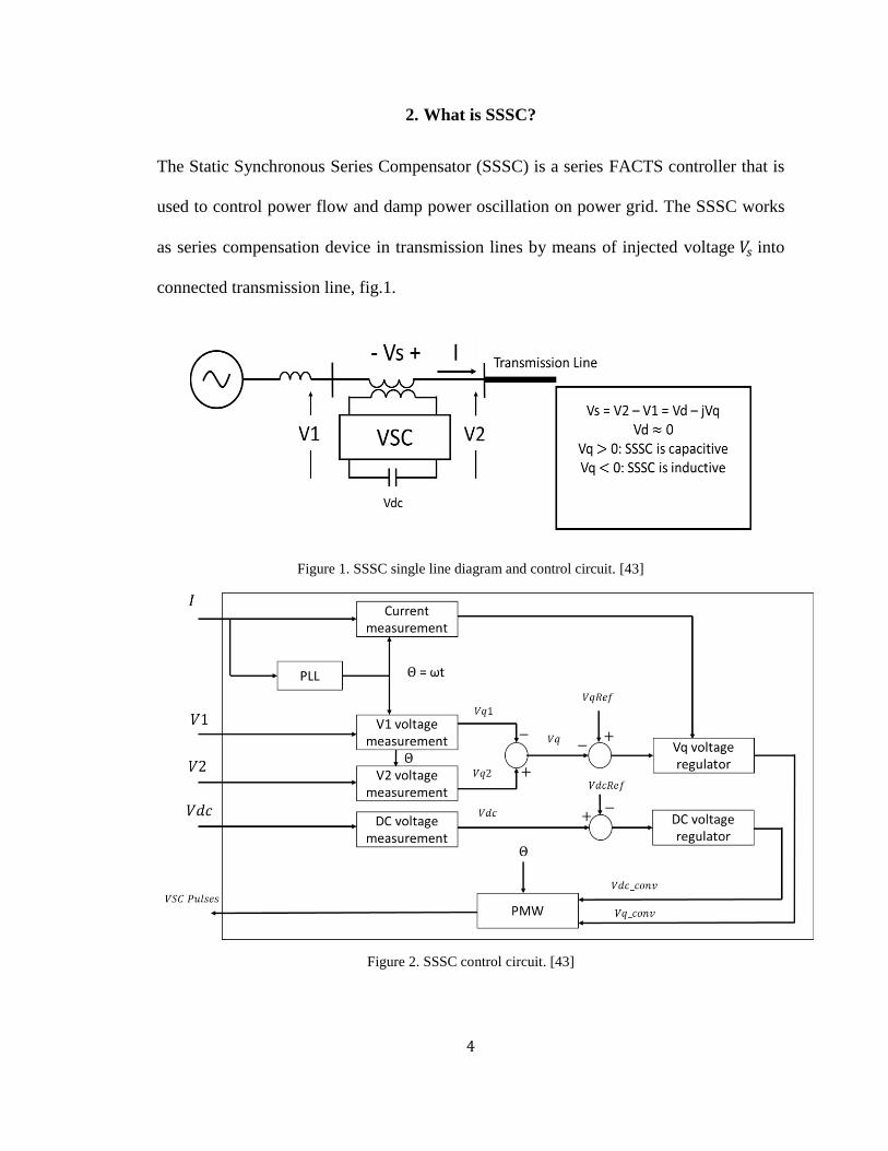
The Static Synchronous Series Compensator (SSSC) is a series FACTS controller that is

used to control power flow and damp power oscillation on power grid. The SSSC works

as series compensation device in transmission lines by means of injected voltage 𝑉𝑠 into

connected transmission line, fig.1.

Figure 1. SSSC single line diagram and control circuit. [43]

Figure 2. SSSC control circuit. [43]

5

Due to lack of thermal, mechanical or renewable energy conversion to generate real

power, injected voltage 𝑉𝑠 must be in quadrature with line current. A distinguishing

feature of SSSC is its ability to resemble both capacitive and inductive compensation.

Alternating magnitude of imaginary ( 𝑉𝑞 ) part of 𝑉𝑠 forms capacitive or inductive as

follows:

𝑉𝑞 > 0, 𝐼𝑛𝑑𝑢𝑐𝑡𝑖𝑣𝑒

𝑉𝑞 < 0, 𝐶𝑎𝑝𝑎𝑐𝑖𝑡𝑖𝑣𝑒

Alternation of 𝑉𝑞 is achieved by Voltage Sourced Converter (VSC) located on low

voltage side of potential transformer in fig.1. GTOs, IGBTs or IGCTs of VSC employs

forced-commutation to create 𝑉𝑑_𝑐𝑜𝑛𝑣 from DC source [43]. Injected voltage 𝑉𝑠 is 90 out

of phase with line current because of active power drawn from grid to supply coupling

transformer with losses and to charge coupling capacitor. VSC in this model consists of

IGBT-based with Pulse-Width Modulation (PWM). PWM synthesizes sinusoidal voltage

from DC voltage at predetermined cutoff frequency in order of kHz. Eventually, 𝑉𝑐𝑜𝑛𝑣 is

changed in response to varying PWM modulation index. The control circuit consists of

phase locked loop (PLL), measurement system and AC&DC voltage regulators. PLL is

locked to positive sequence current of line to calculate line current argument, or phase

(𝜃 = 𝜔𝑡). This argument is compared with grid three phase voltages and currents (𝑉𝑑,

𝑉𝑞 , 𝐼𝑑 , 𝐼𝑞). Measurement blocks measures grid AC three phase components in addition to

DC voltage of coupling capacitor. [43]

6

2.1 SSSC Theory

As explained previously, SSSC is a series compensation device that injects series voltage

in quadrature with line current. Consider simple representation of equivalent circuit

where SSSC is used to compensate between S and R buses, fig.3.

VS, VR = Active power source voltages

Vq = SSSC injected voltage

The real power transfer thru the transmission line is expressed by following formula [18]:

𝑃 = |𝑉𝑆| ∗ |𝑉𝑅|

𝑋𝐿sin 𝛿 +

𝑉

𝑋𝐿𝑉𝑞 cos( 𝛿/2) (1)

𝛿 = power angle between 𝑉𝑆 & 𝑉𝑅

Consequently, SSSC can either increase or decrees real power transfer by means of

alternating of injected voltage Vq between positive and negative respectively, fig.4.

Crucial fact can be read from equation (1) that if Vq has exceeded voltage drop across

uncompensated transmission line reactance 𝑉𝐿, power flow reverses its direction. That is,

power will flow from bus R towards bus S. In stability studies, SSSC has excellent

subcycle response period, also has continuous and smooth transmission between positive

Figure 3. SSSC compensation equivalent circuit. [18]

7

Figure 4. Transmitted power versus compensation voltage Vq.

and negative voltage compensation [18]. As SSSC creates virtual reactance, either

capacitive or inductive, added in series with transmission line, another way of

considering SSSC is adding its reactance to line reactance in power equation. Therefore,

equation (1) becomes: [23, 31]

𝑃 = |𝑉𝑆| ∗ |𝑉𝑅|

𝑋𝐿 ∓ 𝑋𝑆𝑆𝑆𝐶sin 𝛿 (2)

When XL = XSSSC and XSSSC is negative, denominator of equation (2) is zero and hence

power goes infinity in other words becomes unstable. However, series compensation is

usually defined as varying or changing line impedance values to increase/decrease

transmitted power. In practice, series compensation does so by means of enforcing its

voltage across compensated transmission line to increase/decrease line current thus

controlling transmitted power consequently [31].

0 20 40 60 80 100 120 140 160 180-1

-0.5

0

0.5

1

1.5

2

Tra

nsfe

red P

ow

er

in P

U

Power angle in PU

Transmitted Power versus Injected Voltage

Vq = -0.707

Vq = -0.353

Vq = 0

Vq = 0.353

Vq = 0.707

8

2.2 Immunity to Resonance

AC inductor and capacitive impedance is a function of system frequency. In reference to

equation (2), SSSC virtual reactance might react with overall system loading and

impedance to cause sub-frequency or multiple-frequency resonance. If not detected and

critical conditions are met ferroresonance might occur. Sub-frequency resonance is the

most dangerous phenomena due to its severe impact on turbine-generator mechanical

system. At this resonance, electrical system overloads mechanical system and drives it to

resonance in a desperate action to mitigate resonance disturbances [23]. Moreover, Sub-

frequency considers the egestion or first stage of ferroresonance phenomena the most

harmful resonance of all kinds. Contrary to traditional compensation device (capacitor

banks and reactors), SSSC is a voltage source connected in series with transmission line.

By this means, it has fixed injected voltage control output that operates at system

fundamental frequency only. Because of harmonics filters presented in previous section

SSSC harmonics impedances are approximately zero [23].

Although, SSSC contains coupling transformer that has leakage inductance and draws

some real power from grid for that sake. The voltage drop due to this inductance is

reimbursed, or eliminated, by capacitance compensation injected by SSSC. Thus, SSSC

equivalent reactance at all frequencies but fundamental is negligible. Accordingly,

probability of sub-frequency resonance by reason of SSSC compensation very low or

even zero especially in well-designed system. In addition, SSSC provides fast and robust

response to grid disturbances such as faults or post-faults sub-synchronous oscillations.

Actually, this one of prevalent features of SSSC, damping power oscillation, which will

provided later in this project.

9

2.3 SSSC Rating

SSSC injects compensation voltage in quadrature with feeder current. The voltage

magnitude can be either positive or negative. Therefore, SSSC rating can be expressed in

VA as follows:

𝑆𝑆𝑆𝑆𝐶 = √3 ∗ 𝐼 𝐿𝑖𝑛𝑒 𝑀𝑎𝑥 ∗ 𝑉 𝑆𝑆𝑆𝐶 𝑀𝑎𝑥 (𝑉𝐴) (3)

That is, maximum line current multiplied by maximum injected voltage SSSC is capable

of. For instant, SSSC with 1 pu injected voltage has rating of 2 pu VA due to

positive/negative characteristics of SSSC. Yet, the sake of this study is not determine the

optimal rating of SSSC. So that, later in simulation chapter SSSC might be over sized to

limited injected voltage to 10 percent only of nominal voltage. This constrain avoids

overshooting of injected voltage over recommended voltage provided by controller

during system fault. In addition, voltage restrain reduces required time to reach

maximum and desired damping point. This practice will be touched on surface in

simulation chapter.

10

3. Parameters Control

SSSC can effectively control real and reactive power as well as damp power oscillation

during system disturbances. SSSC accepts reference voltage as recommended scalar of

injected voltage. The reference voltage can be real positive or negative only, for inductive

or capacitive compensation. The reference voltage shall follow desired controlled

parameter. For example, when real power is to be controlled in a transmission line, then

input of control circuit shall be real power measured and output, reference voltage, shall

follow the changed in line power in reference to set point. Likewise, derivative of

generator angular velocity (𝑑𝜔), or rate of change in generator angular speed, might be

also fed into control circuit to acquire less generator oscillation in order to avoid out of

synchronism situation.

3.1 Closed Loop Neural Control

Reference [23] proposes control scheme based on neural topology. As illustrated earlier,

SSSC accepts referenced voltage input to be injected by SSSC into compensated line.

This scheme calculates reference voltage as product of line current and recommended

compensating reactance (𝑋𝑞𝑟𝑒𝑓 ). Though, 𝑋𝑞𝑟𝑒𝑓 is hard to anticipate especially with

dynamic grid switching or operation, not to say grid disturbance when SSSC

compensation is mostly needed. In fig.5, first part of control circuit is depicted showing

three terms (𝑚, 𝛽, 𝑘) derived from referenced power values based on following equations.

𝑃𝑖𝑛𝑠𝑡 =3 𝑉𝑑 𝐼𝑑

2 (𝑊) (4)

11

𝑄𝑖𝑛𝑠𝑡 =3 𝑉𝑞 𝐼𝑞

2 (𝑉𝐴𝑅) (5)

Where currents and voltages are peak values not RMS values. Instantaneous power

quantities are calculated in fig.6 using dq0 transformation. From equations (4, 5),

referenced currents are:

𝐼𝑑𝑟𝑒𝑓 =2 𝑃𝑟𝑒𝑓

3 𝑉𝑑 (6)

𝐼𝑞𝑟𝑒𝑓 =2 𝑄𝑟𝑒𝑓

2 𝑉𝑞 (7)

Figure 5. Closed loop neural control first circuit. [23]

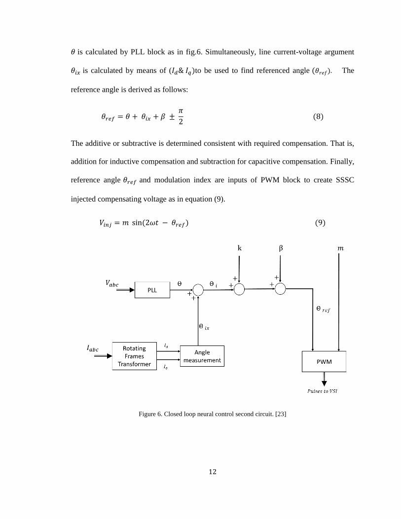
In fig.6, three phase line voltages and currents are measured and transformer into dq0

components. Then measured currents and voltages are compared with calculated ones

derived in fig.5 using equation (6, 7). The error signals are fed into neural controller to

produce displacement angle β and modulation index 𝑚. Instantaneous line voltage angle

12

𝜃 is calculated by PLL block as in fig.6. Simultaneously, line current-voltage argument

𝜃𝑖𝑥 is calculated by means of (𝐼𝑑& 𝐼𝑞)to be used to find referenced angle (𝜃𝑟𝑒𝑓). The

reference angle is derived as follows:

𝜃𝑟𝑒𝑓 = 𝜃 + 𝜃𝑖𝑥 + 𝛽 ± 𝜋

2 (8)

The additive or subtractive is determined consistent with required compensation. That is,

addition for inductive compensation and subtraction for capacitive compensation. Finally,

reference angle 𝜃𝑟𝑒𝑓 and modulation index are inputs of PWM block to create SSSC

injected compensating voltage as in equation (9).

𝑉𝑖𝑛𝑗 = 𝑚 sin(2𝜔𝑡 − 𝜃𝑟𝑒𝑓) (9)

Figure 6. Closed loop neural control second circuit. [23]

13

3.2 Power Oscillation Damper

This kind of control is utilized for damping power oscillation during major disturbances

hence call Power Oscillation Damper (POD). POD controller contains gain block, low-

pass filter, washout (high-pass) filter, r stages of lead-lag (LL) blocks see fig.7.

Figure 7. Power Oscillation Damper (POD) controller. [35]

The transfer function of POD controller is as follows:

𝐻(𝑠) = 𝐾 (1

1 + 𝑠𝑇𝑚) (

𝑠𝑇𝑤

1 + 𝑠𝑇𝑤) (

1 + 𝑠𝑇𝑙𝑒𝑎𝑑

1 + 𝑠𝑇𝑙𝑎𝑔)

𝑟

= 𝐾𝑌(𝑠) (10)

Where 𝐾 is a positive gain, 𝑇𝑚 & 𝑇𝑤 are low-pass and washout filters time constant

respectively. The depicted controller in fig.7 contains two stages lead-lag block

hence 𝑟 = 2, and 𝑇𝑙𝑒𝑎𝑑 & 𝑇𝑙𝑎𝑔 are time constants. The low pass filter is designed to filter

high frequency variance of input signal. The washout acts like a high pass filter to pass

signal oscillation unharmed. Therefore, steady state components in input signal will be

eliminated by reaching (LL) blocks. (LL) blocks works as phase compensator to correct

phase shift occurred due to aforementioned two filters. The setting of POD controller

time constants is in next section.

14

(A) POD Time Constants Calculation and Setting

This section introduces calculation of POD parameters based on eigenvalue value and

instantaneous oscillation angle [30]. SSSC provides dynamic series compensation to

damp power oscillation which means eigenvalue λ must change to match dynamic

compensation. Consequently, ∆𝜆𝑖 must always remain in the left half of the complex

plane for controller stability, fig.8 [30]. The compensation angle (∅𝑐𝑜𝑚𝑝), depicted in

fig.4, is the mandatory shift to line up eigenvalue motion in parallel with negative real

axis. This phase shift is introduced by LL block and its time constants, namely 𝑇𝑙𝑒𝑎𝑑 &

𝑇𝑙𝑎𝑔.

Figure 8. Eigenvalues motion in POD controller. [30]

15

The following equation are used to calculated controller parameter.

∅𝑐𝑜𝑚𝑝 = 180 − 𝑎𝑛𝑔(𝑅𝑖) (11)

𝛼𝑐 =𝑇𝑙𝑒𝑎𝑑

𝑇𝑙𝑎𝑔=

1 − 𝑠𝑖𝑛 (∅𝑐𝑜𝑚𝑝

𝑟 )

1 + 𝑠𝑖𝑛 (∅𝑐𝑜𝑚𝑝

𝑟 )

(12)

𝑇𝑙𝑎𝑔 =1

𝑤𝑖√𝛼𝑐

(13)

𝑇𝑙𝑒𝑎𝑑 = 𝛼𝑐𝑇𝑙𝑎𝑔 (13)

Where (𝑎𝑛𝑔(𝑅𝑖)) denotes phase angle of the system residue oscillation [30]. Then, it is

clear that this design depends substantial on estimation or prediction of oscillation residue

which can be a weakness issue.

(B) Genetic Algorithm Optimization

This section discusses employment of Genetic Algorithm (GA) Optimization to predict or

select fittest values of POD time constants. GA is an optimization, or linearization,

method that has been developed to solve sophisticated mathematical and/or engineering

problems when analytical or numerical methods are not beneficial [45]. As strange as it

sounds to be, GA principle is based on biological evolution and natural selection

mechanism. GA creates and operates population of solutions and selects best solutions

based on the fittest strategy. After that, best individuals, or solutions, are mixed

genetically to reproduce and create new set of solutions. The reproduced children are

considered the fittest individual to survive to next generation (iteration). As generations

advance, individuals shall return better results than their own parents in respect to a

16

fitness function. This process continuous until stopping criteria is met. GA has six major

operator, namely: initialization, selection function, chromosome representation, genetic

operators, termination and fitness function that need to be understood and set prior to

utilization. A brief description of each item are to be followed.

a) Chromosome Representation

Chromosome representation option defines problem structure in GA algorithm engine,

and creates appropriate genetic operators. Chromosome is formed of set of genes

following its nature formation in life. Yet, Chromosome is formed digitally as integers,

floating numbers, binary digits, real numbers, matrices, and etc. depending on sought

solution numbers. Usually, natural representations are effective and yield optimum

solution. Real coded representation is recommended for less computation time [45].

b) Selection Function

Selection function is the most significant factor in GA to produce successive generations

towards the best solution. This function provides survive passports for individuals to

proceed to next generation. It is actually a probabilistic function that evaluates or grades

individuals so that only fittest individuals are chosen. Each software offers several

schemes for section function. For instant, Matlab program provides stochastic uniform,

remainder, uniform, roulette and tournament schemes are available.

c) Genetic Operators

Genetic operators are search tools in GA that create new solution out of past generation

solution. There are two main operators, Crossover and Mutation. Crossover selects pairs

of individuals as parents to produce children (new individuals). Mutation, as it does in

17

nature, modifies parents genes so that newly produced children make different solution

than their own parent once did. Crossover has the following options: constraint

dependent, scattered, single point, two point, intermediate, heuristic, and arithmetic.

Mutation has the following options: constraint dependent, Gaussian, uniform, adaptive

feasible.

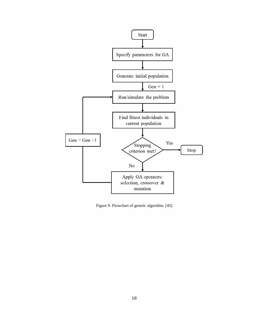
d) Initialization, Termination and Fitness Function

First, a population is required to start GA procedure. Usually GA chooses lower limits of

user input variables otherwise, initial population is chosen randomly. GA continuously

starts new generation after a generation unless a stopping criterion is satisfied. There are

several stopping conditions are available such as population convergence, maximum

number of generations, solution cannot be improved, and a target value of problem

function is found. Fitness function is the function entered by user that GA uses to

evaluate individuals, or solutions, in order to compare and thus select best solutions. Such

a function could be an error signal in PID controller for simple step input signal. Fig.9 is

flowchart summarizes GA steps.

18

Figure 9. Flowchart of genetic algorithm. [45]

19

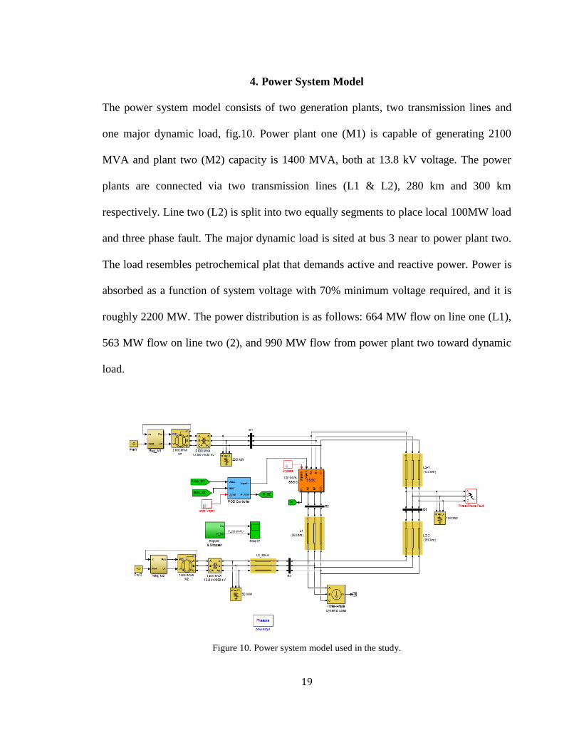
4. Power System Model

The power system model consists of two generation plants, two transmission lines and

one major dynamic load, fig.10. Power plant one (M1) is capable of generating 2100

MVA and plant two (M2) capacity is 1400 MVA, both at 13.8 kV voltage. The power

plants are connected via two transmission lines (L1 & L2), 280 km and 300 km

respectively. Line two (L2) is split into two equally segments to place local 100MW load

and three phase fault. The major dynamic load is sited at bus 3 near to power plant two.

The load resembles petrochemical plat that demands active and reactive power. Power is

absorbed as a function of system voltage with 70% minimum voltage required, and it is

roughly 2200 MW. The power distribution is as follows: 664 MW flow on line one (L1),

563 MW flow on line two (2), and 990 MW flow from power plant two toward dynamic

load.

Figure 10. Power system model used in the study.

20

SSSC rating can be calculated using equation (3) in chapter 2, with maximum 𝑉 𝑆𝑆𝑆𝐶

chosen to be 10 percent and line current is measured from model.

𝑉 𝑆𝑆𝑆𝐶 = 0.1 ∗ 500𝑘 = 50 𝑘𝑉

𝐼 𝑙𝑖𝑛𝑒 ≅ 6.7 ∗ (100𝑀

√3 ∗ 500𝑘) = 774 𝐴𝑚𝑝

𝑆𝑆𝑆𝑆𝐶 = √3 ∗ 𝐼 𝑙𝑖𝑛𝑒 ∗ 𝑉 𝑆𝑆𝑆𝐶 = 67 MVA

Yet, SSSC is chosen to be 100 MVA, that to minimize injected voltage into the grid as

much as possible. Also, it serves stability as it minimize injected voltage rate of change in

respect to time, that is to say how fast SSSC response is. Rapid SSSC response has a

number of disadvantages one of which is oscillation at system dynamic instants. Full

description of each block will be given later in appendix A.

Control circuit contains L1 real power transfer measured at bus 2, simple PID controller

and one stage LL controller.

Figure 11. Case one control circuit.

21

4.1 Case 1: Varying Real Power

This case study demonstrations model validity and then SSSC ability to control power

transfer in line one. This case consists of three simulations: system without SSSC, L1

power is increases to 700 MW by SSSC and L1 power is decrease to 600MW by SSSC.

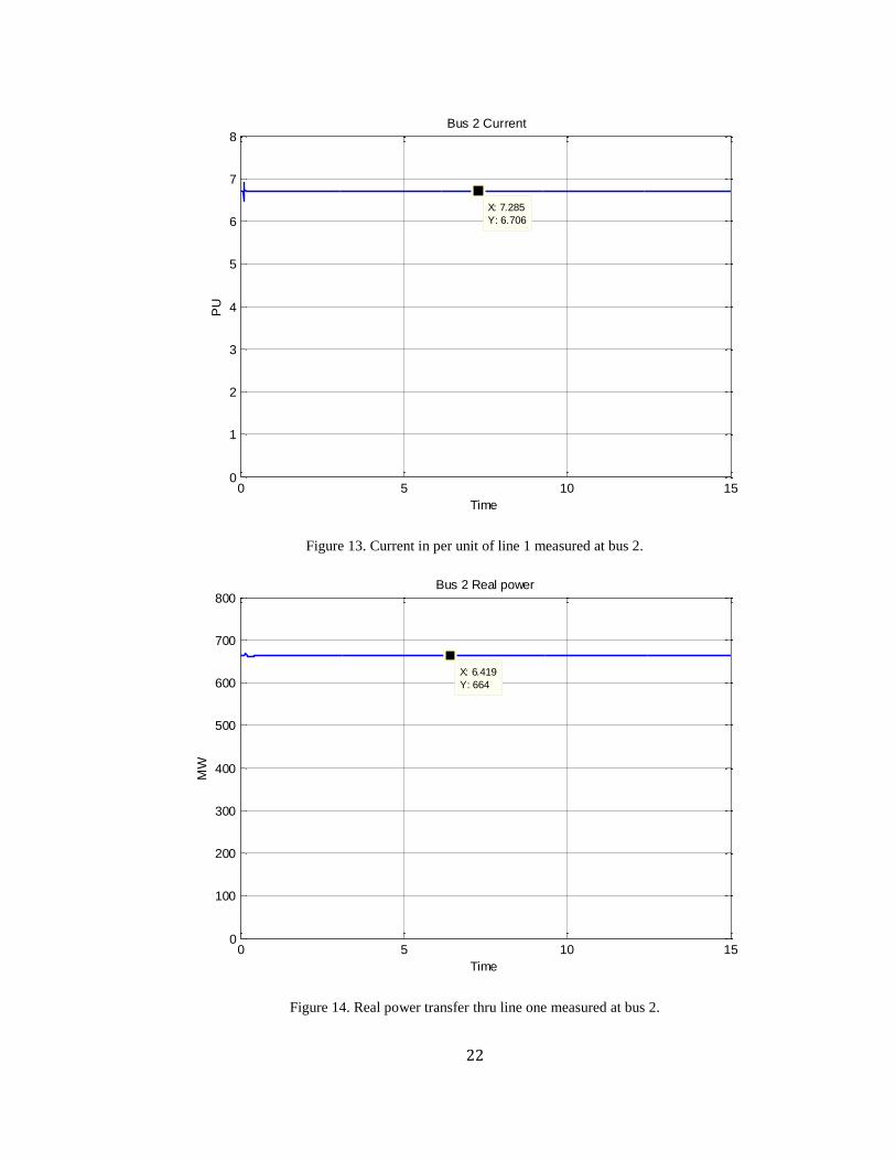
(A) Simulation One: system validity

Figure 12. Voltage profile in per unit measured at bus 1.

0 5 10 150

0.5

1

1.5

X: 8.09

Y: 1.007

Bus 2 Voltage

Time

PU

22

Figure 13. Current in per unit of line 1 measured at bus 2.

Figure 14. Real power transfer thru line one measured at bus 2.

0 5 10 150

1

2

3

4

5

6

7

8

X: 7.285

Y: 6.706

Bus 2 Current

Time

PU

0 5 10 150

100

200

300

400

500

600

700

800

X: 6.419

Y: 664

Bus 2 Real power

Time

MW

23

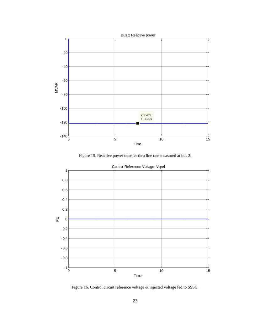
Figure 15. Reactive power transfer thru line one measured at bus 2.

Figure 16. Control circuit reference voltage & injected voltage fed to SSSC.

0 5 10 15-140

-120

-100

-80

-60

-40

-20

0

X: 7.455

Y: -121.9

Bus 2 Reactive power

Time

MV

AR

0 5 10 15-1

-0.8

-0.6

-0.4

-0.2

0

0.2

0.4

0.6

0.8

1Control Reference Voltage Vqref

Time

PU

24

(B) Simulation Two: L1 power = 700 MW



0 5 10 150.99

0.995

1

1.005

1.01

1.015

1.02

1.025

X: 7.948

Y: 1.002

Bus 2 Voltage

Time

PU

No SSSC

SSSC

0 5 10 156.4

6.5

6.6

6.7

6.8

6.9

7

7.1

7.2

X: 7.341

Y: 7.091

Bus 2 Current

Time

PU

No SSSC

SSSC

25



0 5 10 15660

665

670

675

680

685

690

695

700

705

X: 6.916

Y: 700

Bus 2 Real power

Time

MW

No SSSC

SSSC

0 5 10 15-140

-120

-100

-80

-60

-40

-20

0Bus 2 Reactive power

Time

MV

AR

No SSSC

SSSC

26

Figure 21. Control circuit referenced voltage & injected voltage fed to grid.

Note that in fig.21 𝑉𝑞𝑟𝑒𝑓 is the control circuit reference signal to SSSC and 𝑉𝑞𝑖𝑛𝑗 is the

actual injected voltage to grid. Here is a brief calculation of SSSC compensation to L1.

Even though SSSC injected voltage to system is depicted in Fig.21, resultant power

cannot be calculated using fig.21 only. SSSC compensation changes three main

parameters that shall be encountered to correctly get transferred power. Transmission line

sending end voltage, receiving end voltage and equivalent impedance are ought to be

used in equation (2). These three values are obtained from model simulation as follows.

|𝑉 𝑏𝑢𝑠1| = 1.0087 𝑝𝑢

|𝑉 𝑏𝑢𝑠2| = 1.0011 𝑝𝑢

|𝑋 𝑙𝑖𝑛𝑒 ∓ 𝑋 𝑆𝑆𝑆𝐶| = 0.0338 𝑝𝑢

𝛿12 = 𝜃(𝑉 𝑏𝑢𝑠1) − 𝜃(𝑉 𝑏𝑢𝑠2) = 13.6839 𝑑𝑒𝑔

0 5 10 15-0.005

0

0.005

0.01

0.015

0.02

0.025

0.03

0.035SSSC Injected Voltage Vqinj

Time

PU

Vqref

Vqinj

27

Substituting in equation (2):

𝑃 = (1.0087) ∗ (1.0011)

0.0338sin(13.6839) = 7.07 𝑝𝑢 ≈ 700 𝑀𝑊

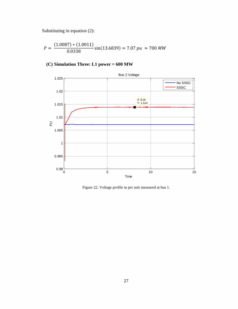
(C) Simulation Three: L1 power = 600 MW


0 5 10 150.99

0.995

1

1.005

1.01

1.015

1.02

1.025

X: 8.16

Y: 1.014

Bus 2 Voltage

Time

PU

No SSSC

SSSC

28



0 5 10 156

6.1

6.2

6.3

6.4

6.5

6.6

6.7

6.8

6.9

7

X: 8.712

Y: 6.035

Bus 2 Current

Time

PU

No SSSC

SSSC

0 5 10 15590

600

610

620

630

640

650

660

670

X: 7.48

Y: 600

Bus 2 Real power

Time

MW

No SSSC

SSSC

29



0 5 10 15-140

-120

-100

-80

-60

-40

-20

0Bus 2 Reactive power

Time

MV

AR

No SSSC

SSSC

0 5 10 15-0.06

-0.05

-0.04

-0.03

-0.02

-0.01

0


Time

PU

Vqref

Vqinj

30

4.2 Case 2: Damping L1 Real Power

After validation of SSSC ability to control real power, this case shows another crucial

feature of SSSC that is power damping during severe power system faults. The Same

model in previous case is used with three-phase-fault applied at 1.333 seconds and

cleared at 1.5 seconds. The fault location is the same as in fig.10 at the middle of line

two. A disturbance, or oscillation, is a deviation of instantaneous power from a designed

or preferred set point, thus (𝑃𝑖𝑛𝑠𝑡 − 𝑃𝑝𝑟𝑒𝑓 ) can be used as an error signal. Hence,

minimizing the error signal leads to minimum power oscillation. In addition, an

integration over simulation time of absolute error signal delivers better result than using

error signal only. The objective equation becomes:

𝐸 = ∫ |𝑃𝑖𝑛𝑠𝑡 − 𝑃𝑝𝑟𝑒𝑓|

𝑡𝑠𝑖𝑚

0

𝑑𝑡 (14)

GA tool will be used to tune Lead-Lag parameters to find minimum value of equation

(14). GA is the best candidate because it employs advance algorithm in a search of fittest

parameters that returns minimum error value. GA runs in generations, or iterations, at

which a group of possible solutions are tested in the system model and fitness function

value is recorded. GA stops when maximum number of generation is exceeded or when a

desired value of fitness function is met. Such a feature makes GA a simulation of

scientific empiricism. GA simulation that runs 100 generations is worth hundred years of

real life experience. GA is designed to minimize equation (14) subjected to following

constrains:

𝐾𝑚𝑖𝑛 ≤ 𝐾 ≤ 𝐾𝑚𝑎𝑥 (15)

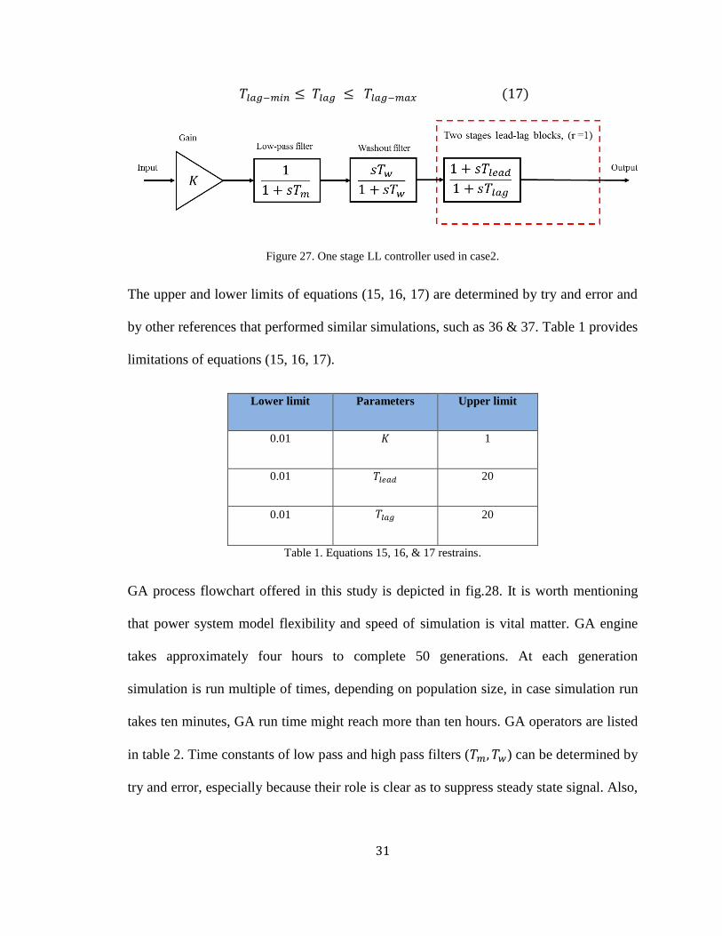
𝑇𝑙𝑒𝑎𝑑−𝑚𝑖𝑛 ≤ 𝑇𝑙𝑒𝑎𝑑 ≤ 𝑇𝑙𝑒𝑎𝑑−𝑚𝑎𝑥 (16)

31

𝑇𝑙𝑎𝑔−𝑚𝑖𝑛 ≤ 𝑇𝑙𝑎𝑔 ≤ 𝑇𝑙𝑎𝑔−𝑚𝑎𝑥 (17)

Figure 27. One stage LL controller used in case2.

The upper and lower limits of equations (15, 16, 17) are determined by try and error and

by other references that performed similar simulations, such as 36 & 37. Table 1 provides

limitations of equations (15, 16, 17).

Lower limit Parameters Upper limit

0.01 𝐾 1

0.01 𝑇𝑙𝑒𝑎𝑑 20

0.01 𝑇𝑙𝑎𝑔 20

Table 1. Equations 15, 16, & 17 restrains.

GA process flowchart offered in this study is depicted in fig.28. It is worth mentioning

that power system model flexibility and speed of simulation is vital matter. GA engine

takes approximately four hours to complete 50 generations. At each generation

simulation is run multiple of times, depending on population size, in case simulation run

takes ten minutes, GA run time might reach more than ten hours. GA operators are listed

in table 2. Time constants of low pass and high pass filters (𝑇𝑚, 𝑇𝑤) can be determined by

try and error, especially because their role is clear as to suppress steady state signal. Also,

32

some references, e.g. 35, 36, 45, suggest that (𝑇𝑚, 𝑇𝑤) values might be in rage of [0 to

0.1] and [1 to 10] respectively. In this case [1e-6, 1] are used for (𝑇𝑚, 𝑇𝑤).

Figure 28. GA flowchart process.

GA Operators Setting

Operator Setting

Population size 50

Fitness scaling Rank

Selection function Uniform

Mutation Constraint dependent

Crossover function Arithmetic

Generations 50

Table 2. GA operators setting

33

Fitness function convergence graph is shown in fig.29, generated from GA tool. The

figure shows fitness function, equation (14), best value for each generation along with

average value for all population size. A fitness function goes to convergence when mean

value matches or come in contact with best value.

Figure 29. Fitness function convergence.

The final solution parameters are tabulated in table 3.

Parameters 𝐾 𝑇𝑙𝑒𝑎𝑑 𝑇𝑙𝑎𝑔

Final Value 0.08 15.759 7.332

Table 3. GA final solutions.

The resultant damping behavior of SSSC is outstanding, fig.30. Line power drops to

almost 200 MW during fault while with SSSC compensation it barely reaches 280 MW.

After clearing fault, line power overshoots passing 900 MW and goes under 700 MW

after 2.4 seconds after which it continue oscillating until 7 seconds. Whereas, when

0 5 10 15 20 25 30 35 40 45 501

2

3

4

5

6

7

8

9

10x 10

4

Generation

Fitness v

alu

e

Best: 16308.4 Mean: 17322.8

Best f itness

Mean fitness

34

compensation is in active it rapidly damps down below 700 at ~ 1.6 second, and then

smoothly reaches nominal line power (664 MW) with oscillation free manner.

Figure 30. Power response to 3Q fault with/out SSSC measured at bus 2.

0 1 2 3 4 5 6 7 8 9 10200

300

400

500

600

700

800

900

1000Bus 2 Real power

Time

MW

No SSSC

SSSC

35


4.3 Case 3: Damping Rotor Oscillation and Line Power

Power system disturbance affects multiple parameters, like power quantity, power

quality, power angle and generator rotor speed. Compensation that minimize deviation in

any, or all, aforementioned parameters leads to quicker damping of oscillation. This study

seeks damping rotor speed as well as line power instantaneously.

(A) Damping Rotor Speed

First, let seek damping rotor oscillation. A fitness function shall be identified to measure

rotor speed deviation due to a disturbance. The chosen function is an integration of

absolute difference between generators angular speed times simulation time period [45].

The fitness function is expressed in equation (18).

𝐷 = ∫ |∆𝜔1 − ∆𝜔2| ∗ 𝑡 𝑑𝑡𝑡𝑠𝑖𝑚

0

(18)

0 1 2 3 4 5 6 7 8 9 10-0.2

-0.15

-0.1

-0.05

0

0.05

0.1


Time

PU

Vqref

Vqinj

36

Where (∆𝜔1, ∆𝜔2) are speed deviation of generator one and two respectively. Simulation

goal to find minimum value of equation (18) aiming to enhance system response to

disturbances. The controller is two stages lead-Lag controller similar to fig. 7. The

controller circuit is given in table 4.

Figure 32. Rotor speed damper control circuit.

Rotor speed damper controller

Constants Value

Gain, K [10-500], To be determined by GA

Sensor, 𝑇𝑠 0.001

Washout filter, 𝑇𝑤 10

LL#1, 𝑇1𝑛 , 𝑇1𝑑 [.01-3], To be determined by GA

LL#2, 𝑇2𝑛 , 𝑇2𝑑 [.01-3], To be determined by GA

Table 4. Rotor speed damper controller parameters.

GA is employed to determine controller constants same way it has been used in case. GA

process flowchart and operators are given in fig.28 and table 2 respectively with 60

generations instead of 50.

37


Fitness function is depicted in fig.33 showing fast and consistent convergence. The final

solution values and figures are as follows.

Parameters 𝐾 𝑇1𝑛 𝑇1𝑑 𝑇2𝑛 𝑇2𝑑

Final Value 300.243 0.0899 0.35 2.88 0.88


0 10 20 30 40 50 602.5

3

3.5

4

4.5

5

5.5

6

6.5

7

7.5

Generation

Fitness v

alu

e

Best: 2.60577 Mean: 2.71153

Best f itness

Mean fitness

38

Figure 34. Rotor speed deviation response with SSSC damping.


0 1 2 3 4 5 6 7 8-4

-3

-2

-1

0

1

2

3x 10

-3dw1 - dw2

Time

rad/s

ec

No SSSC

SSSC

0 1 2 3 4 5 6 7 8-0.2

-0.15

-0.1

-0.05

0

0.05

0.1

0.15


Time

PU

Vqref

Vqinj

39

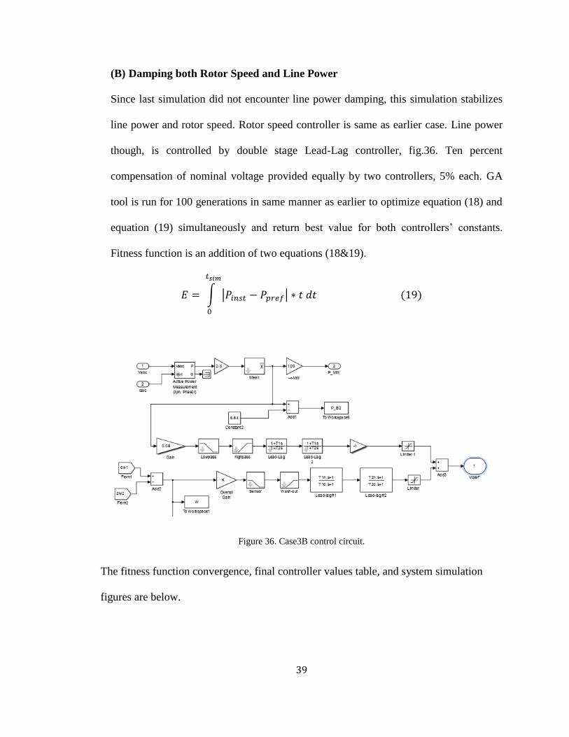
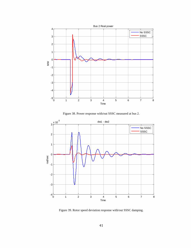
(B) Damping both Rotor Speed and Line Power

Since last simulation did not encounter line power damping, this simulation stabilizes

line power and rotor speed. Rotor speed controller is same as earlier case. Line power

though, is controlled by double stage Lead-Lag controller, fig.36. Ten percent

compensation of nominal voltage provided equally by two controllers, 5% each. GA

tool is run for 100 generations in same manner as earlier to optimize equation (18) and

equation (19) simultaneously and return best value for both controllers’ constants.

Fitness function is an addition of two equations (18&19).

𝐸 = ∫ |𝑃𝑖𝑛𝑠𝑡 − 𝑃𝑝𝑟𝑒𝑓|

𝑡𝑠𝑖𝑚

0

∗ 𝑡 𝑑𝑡 (19)

Figure 36. Case3B control circuit.

The fitness function convergence, final controller values table, and system simulation

figures are below.

40


Fitness function is depicted in fig.37 showing fast and consistent convergence. The final

solution values and figures are as follows.

Power damper controller Rotor damper controller

K 0.08 K 104.027

LL#1, 𝑇1𝑛 0.619 LL#1, 𝑇1𝑛 0.599

LL#1, 𝑇1𝑑 0.381 LL#1, 𝑇1𝑑 0.664

LL#2, 𝑇1𝑛 0.688 LL#2, 𝑇1𝑛 0.454

LL#2, 𝑇2𝑑 0.69 LL#2, 𝑇2𝑑 0.353


0 10 20 30 40 50 60 70 80 90 1004.4

4.6

4.8

5

5.2

5.4

5.6

5.8

6

6.2

6.4x 10

4

Generation

Fitness v

alu

e

Best: 44455.8 Mean: 45577.7

Best f itness

Mean fitness

41

Figure 38. Power response with/out SSSC measured at bus 2.

Figure 39. Rotor speed deviation response with/out SSSC damping.

0 1 2 3 4 5 6 7 8-5

-4

-3

-2

-1

0

1

2

3

4Bus 2 Real power

Time

MW

No SSSC

SSSC

0 1 2 3 4 5 6 7 8-4

-3

-2

-1

0

1

2

3x 10

-3dw1 - dw2

Time

rad/s

ec

No SSSC

SSSC

42


4.4 Results and Discussion

Three simulation cases have been carried out on SSSC transmission line compensation

objective. The first case was only demonstration of SSSC capability during normal

operation, showing only power transfer control for particular set points. Last two, SSSC

has been employed to damping power transfer and generator speed during system

disturbances. Study cases utilized lead-lag controller for damping and PID controller to

control line power transfer. Two types of lead-lag controller was used, stage one and

stage two. Stage one was effective in damping transferred power thru transmission line.

The reason behind that is input signal, or error signal, was integer numbers. Also, that’s

why gain value was very small (0.08). The case proves that lead-lag controller structure is

very sensitive hence effective in detection power deviation or disturbance. When power

0 1 2 3 4 5 6 7 8-0.2

-0.15

-0.1

-0.05

0

0.05

0.1


Time

PU

Vqref

Vqinj

43

remains fixed or in steady state condition no compensation is injected. Case two is a solid

evidence on SSSC capability of limiting power drop during faults and elimination of post

fault oscillations. On other hand, small error signal and fast oscillations require two stage

lead-lag controller, as in case two. Final case shows SSSC flexibility to control two

deviations at same time, power line and rotor speed. Therefore, SSSC can be used to

serve multiple tasks such as power factor correction, maximize power transfer and

generator oscillations.

44

5. Conclusion

Due to Vast and fast development of industry and population impose huge increase in

power demand. Not only new power generation is needed but also transmission line

capacity has to be upgraded to match proportional demand. SSSC is a series FACTS

device that used for transmission line compensate to control transferred power and damp

system oscillations during disturbances. The scope of this project is to demonstrate

behavior and applications of SSSC in power system. Three simulation cases have been

carried out in Matlab Simulink tool. The cases have been carried out on power system

model with SSSC installed in series with transmission line. The first case was only

demonstration of SSSC capability during normal operation, showing only power transfer

control for particular set points. Last two, SSSC has been employed to damping power

transfer and generator speed during system disturbances. Achieved results are in approval

with theoretical predictions of device functioning and capability. SSSC behavior in

different conditions was outstanding in all cases. Lead-Lag controller was used in two

kinds, stage one and two. GA tool was employed to optimize selected fitness function,

usually error signal, to tune controller constants. GA tool optimization improves SSSC

compensation performance and hence power system oscillations are successfully

eliminated or damped out even during severe faults conditions. Finally, fast and dynamic

response qualifies SSSC for further research and improvement to meet desired system

disturbance damping and power controlling.

45

Bibliography

[1] Gjerde, J.O., et al, “Use of HVDC and FACTS-components for enhancement of power system

stability”, Electrotechnical Conference, 1996. MELECON '96., 8th Mediterranean

[2] Wang, Y., et al, “Power System Load Modeling”, Power System Technology, 1998. Proceedings.

POWERCON '98. 1998 International Conference

[3] Reed, G.F., et al, “Applications of Voltage Source Inverter (VSI) Based Technology for FACTS

and Custom Power Installations”, Power System Technology, 2000. Proceedings. PowerCon

2000. International Conference

[4] Moran, L., “Power Electronics Applications in Utility Systems”, Industrial Electronics Society,

2003. IECON '03. The 29th Annual Conference of the IEEE

[5] Milano, F., “An Open Source Power System Analysis Toolbox”, Power Systems, IEEE

Transactions, Aug. 2005

[6] Oskoui, A., et al, “Holly STATCOM - FACTS to Replace Critical Generation, Operational

Experience”, Po Transmission and Distribution Conference and Exhibition, 2005/2006 IEEE PES

[7] Sullivan, D., “Design and Application of a Static VAR Compensator for Voltage Support in the

Dublin, Georgia Area”, Transmission and Distribution Conference and Exhibition, 2005/2006

IEEE PES

[8] Pourbeik, P., et al, “Operational Experiences with SVCs for Local and Remote Disturbances”,

Power Systems Conference and Exposition, 2006. PSCE '06. 2006 IEEE PES

[9] Kowalski, J., et al, “Application of Static VAR Compensation on the Southern California Edison

System to Improve Transmission System Capacity and Address Voltage Stability Issues - Part 1.

Planning, Design and Performance Criteria Considerations”, Power Systems Conference and

Exposition, 2006. PSCE '06. 2006 IEEE PES

http://ieeexplore.ieee.org/search/searchresult.jsp?searchWithin=p_Authors:.QT.Gjerde,%20J.O..QT.&searchWithin=p_Author_Ids:37348692200&newsearch=true

46

[10] Sullivan, D., et al, “Voltage Control in Southwest UtahWith the St. George Static Var System”,

Power Systems Conference and Exposition, 2006. PSCE '06. 2006 IEEE PES

[11] Hassink, P., et al, “Dynamic Reactive Compensation System for Wind Generation Hub”, Power

Systems Conference and Exposition, 2006. PSCE '06. 2006 IEEE PES

[12] Poshtan, M., Singh, B.N., Rastgoufard, P., “A Nonlinear Control Method for SSSC to Improve

Power System Stability”, Power Electronics, Drives and Energy Systems, 2006. PEDES '06.

International Conference

[13] Paserba, J., “Recent Power Electronics/FACTS Installations to Improve Power System Dynamic

Performance”, Power Engineering Society General Meeting, 2007. IEEE

[14] Huang, A.Q., et al, “Active Power Management of Electric Power System Using Emerging Power

Electronics Technology”, Power Engineering Society General Meeting, 2007. IEEE

[15] Kumar, N., et al, “Damping Subsynchronous Oscillations in Power System Using Shunt and Series

Connected FACTS Controllers”, Power, Control and Embedded Systems (ICPCES), 2010


[16] Aggarwal, G., et al, “MATLAB/Simulink Based Simulation of a Hybrid Power Flow Controller”,

Advanced Computing & Communication Technologies (ACCT), 2014 Fourth International

Conference

[17] Dejvises, J., Green, T.C., “Control of a Unified Power Flow Controller in Fault Recovery and

With Harmonic Filter”, Power Electronics and Variable Speed Drives, 2000. Eighth International

Conference

[18] Saraf, N., et al. “A Model of the Static Synchronous Series Compensator for the Real Time Digital

Simulator”, Future Power Systems, 2005 International Conference

47

[19] Liu Qing, et al, “Study and Simulation of SSSC and TCSC Transient Control Performance”, Power

System Technology and IEEE Power India Conference, 2008. POWERCON 2008. Joint


[20] Ye, Y., et al, “Current-Source Converter Based SSSC: Modeling and Control”, Power

Engineering Society Summer Meeting, 2001

[21] Vyakaranam, B., et al, “Dynamic Harmonic Evolution in FACTS via the Extended Harmonic

Domain Method”, Power and Energy Conference at Illinois (PECI), 2010

[22] Sarvi, G.A., Bina, M.T., “SSSC Circuit Model for Three-wire Systems Coupled with Delta-

Connected Transformer”, Power and Energy Engineering Conference (APPEEC), 2010 Asia-

Pacific

[23] Padma, S., et al., “Neural Network Controller for Static Synchronous Series Compensator (SSSC)

in Transient Stability Analysis”, Power Electronics (IICPE), 2010 India International Conference

[24] Faridi, M., et al., “Power System Stability Enhancement Using Static Synchronous Series

Compensator (SSSC)”, Computer Research and Development (ICCRD), 2011 3rd International

Conference

[25] Raphael, S., Massoud, A.M., “Static Synchronous Series Compensator for Low Voltage Ride

Through Capability of Wind Energy Systems”, Renewable Power Generation (RPG 2011), IET

Conference

[26] Muruganandham, J., Gnanadass, R., “Performance Analysis of Interline Power Flow Controller

for Practical Power System”, Electrical, Electronics and Computer Science (SCEECS), 2012

IEEE Students' Conference

[27] Kumar, S.A., “Multi Machine Power System Stability Enhancement Using Static Synchronous

Series Compensator (SSSC)”, Computing, Electronics and Electrical Technologies (ICCEET),

2012 International Conference

48

[28] Li Wang, Quang-Son Vo, “Power Flow Control and Stability Improvement of Connecting an

Offshore Wind Farm to a One-Machine Infinite-Bus System Using a Static Synchronous Series

Compensator”, Sustainable Energy, IEEE Transactions, April 2013

[29] Kamboj, N., et al, “A Comparative Study of Damping Subsynchronous Resonance Using SSSC and

STATCOM”, Power Electronics (IICPE), 2012 IEEE 5th India International Conference

[30] Anwer, N., et al, “Analysis of UPFC, SSSC with and without POD in Congestion Management of

Transmission System”, Power Electronics (IICPE), 2012 IEEE 5th India International Conference

[31] Gyugyi, Laszlo, et al, “Static Synchronous Series Compensator: A Solid-State Approach to the

Series Compensation of Transmission Lines”, Power Engineering Review, IEEE, Jan 1997

[32] Faried, S.O., et al, “The Use of Static Synchronous Series Compensator for Improving Power

System Stability in Response to Selective-Pole Switching”, Innovative Smart Grid Technologies

Conference Europe (ISGT Europe), 2010 IEEE PES

[33] Ugalde-Loo, C.E., et al, “Comparison between Series and Shunt FACTS Controllers using

Individual Channel Analysis and Design”, Universities Power Engineering Conference (UPEC),

2010 45th International

[34] Chauhan, Y.K., et al, “Performance of a Three-Phase Self-Excited Induction Generator with Static

Synchronous Series Compensator”, Power Electronics, Drives and Energy Systems (PEDES) &

2010 Power India, 2010 Joint International Conference

[35] Taheri, H., et al, “Application of Synchronous Static Series Compensator (SSSC) on Enhancement

of Voltage Stability and Power Oscillation Damping”, EUROCON 2009, EUROCON '09. IEEE

[36] Su, Chi, Chen, Zhe, “Damping Inter-Area Oscillations Using Static Synchronous Series

Compensator (SSSC)”, Universities' Power Engineering Conference (UPEC), Proceedings of 2011

46th International

49

[37] Narne, R., “Damping of Inter-area Oscillations in Power System using Genetic Optimization

Based Coordinated PSS with FACTS Stabilizers”, India Conference (INDICON), 2012 Annual

IEEE

[38] Narne, R., Panda, P.C., “Optimal Coordinate Control of PSS with Series and Shunt FACTS

Stabilizers for Damping Power Oscillations”, Power Electronics, Drives and Energy Systems

(PEDES), 2012 IEEE International Conference

[39] Weihao Hu, et al “Comparison Study of Power System Small Signal Stability Improvement Using

SSSC and STATCOM”, Industrial Electronics Society, IECON 2013 - 39th Annual Conference of

the IEEE

[40] Kotwal, C., et al “Improving Power Oscillation Damping Using Static Synchronous Series

Compensator”, India Conference (INDICON), 2013 Annual IEEE

[41] Georgilakis, P., Vernados, P., “Flexible AC Transmission System Controllers: An Evaluation”,

Materials Science Forum, Trans Tech Publications, Switzerland, 2011

[42] Kumar, P., et al, “Static Synchronous series Compensator for Series Compensation of EHV

Transmission Line”, International Journal of Advanced Research in Electrical, Electronics and

Instrumentation Engineering, Vol. 2, Issue 7, July 2013

[43] Mathworks Inc, website.

<http://www.mathworks.com/help/physmod/sps/powersys/ref/staticsynchronousseriescompensator

phasortype.html?searchHighlight=SSSC>

[44] Falehi, A.D. et al, “Coordinated design of PSSs and SSSC-based damping controller based on GA

optimization technique for damping of power system multi-mode oscillations”, Power Electronics,

Drive Systems and Technologies Conference (PEDSTC), 2011

[45] Panda, G., Rautraya, P., “Damping of Oscillations in Multi Machine Integrated Power Systems by

SSSC Based Damping Controller Employing Modified Genetic Algorithms”, International Journal

of Electrical, Computer, Electronics and Communication Engineering Vol:8 No:2, 2014

50

Appendix A

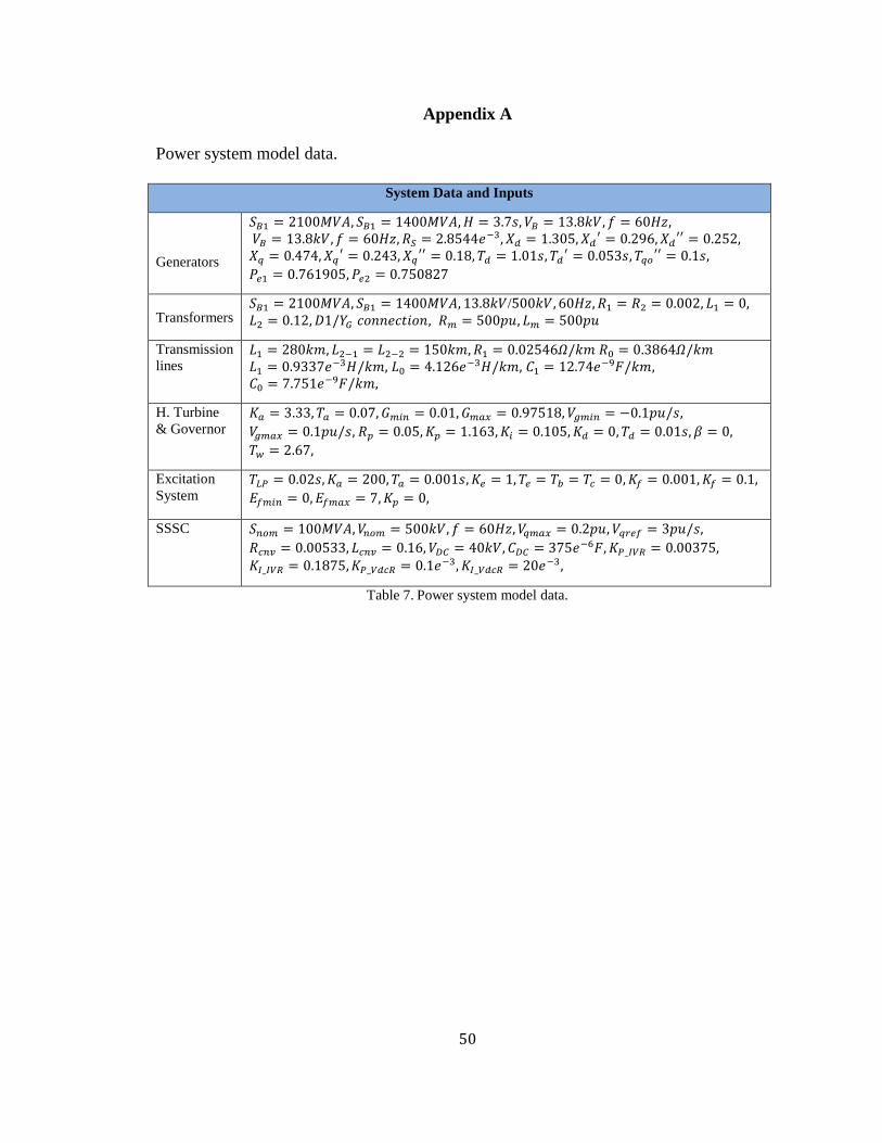
Power system model data.

System Data and Inputs

Generators

𝑆𝐵1 = 2100𝑀𝑉𝐴, 𝑆𝐵1 = 1400𝑀𝑉𝐴, 𝐻 = 3.7𝑠, 𝑉𝐵 = 13.8𝑘𝑉, 𝑓 = 60𝐻𝑧, 𝑉𝐵 = 13.8𝑘𝑉, 𝑓 = 60𝐻𝑧, 𝑅𝑆 = 2.8544𝑒−3, 𝑋𝑑 = 1.305, 𝑋𝑑

′ = 0.296, 𝑋𝑑′′ = 0.252,

𝑋𝑞 = 0.474, 𝑋𝑞′ = 0.243, 𝑋𝑞

′′ = 0.18, 𝑇𝑑 = 1.01𝑠, 𝑇𝑑′ = 0.053𝑠, 𝑇𝑞𝑜

′′ = 0.1𝑠,

𝑃𝑒1 = 0.761905, 𝑃𝑒2 = 0.750827

Transformers 𝑆𝐵1 = 2100𝑀𝑉𝐴, 𝑆𝐵1 = 1400𝑀𝑉𝐴, 13.8𝑘𝑉/500𝑘𝑉, 60𝐻𝑧, 𝑅1 = 𝑅2 = 0.002, 𝐿1 = 0, 𝐿2 = 0.12, 𝐷1/𝑌𝐺 𝑐𝑜𝑛𝑛𝑒𝑐𝑡𝑖𝑜𝑛, 𝑅𝑚 = 500𝑝𝑢, 𝐿𝑚 = 500𝑝𝑢

Transmission

lines 𝐿1 = 280𝑘𝑚, 𝐿2−1 = 𝐿2−2 = 150𝑘𝑚, 𝑅1 = 0.02546𝛺/𝑘𝑚 𝑅0 = 0.3864𝛺/𝑘𝑚

𝐿1 = 0.9337𝑒−3𝐻/𝑘𝑚, 𝐿0 = 4.126𝑒−3𝐻/𝑘𝑚, 𝐶1 = 12.74𝑒−9𝐹/𝑘𝑚, 𝐶0 = 7.751𝑒−9𝐹/𝑘𝑚,

H. Turbine

& Governor 𝐾𝑎 = 3.33, 𝑇𝑎 = 0.07, 𝐺𝑚𝑖𝑛 = 0.01, 𝐺𝑚𝑎𝑥 = 0.97518, 𝑉𝑔𝑚𝑖𝑛 = −0.1𝑝𝑢/𝑠, 𝑉𝑔𝑚𝑎𝑥 = 0.1𝑝𝑢/𝑠, 𝑅𝑝 = 0.05, 𝐾𝑝 = 1.163, 𝐾𝑖 = 0.105, 𝐾𝑑 = 0, 𝑇𝑑 = 0.01𝑠, 𝛽 = 0, 𝑇𝑤 = 2.67,

Excitation

System 𝑇𝐿𝑃 = 0.02𝑠, 𝐾𝑎 = 200, 𝑇𝑎 = 0.001𝑠, 𝐾𝑒 = 1, 𝑇𝑒 = 𝑇𝑏 = 𝑇𝑐 = 0, 𝐾𝑓 = 0.001, 𝐾𝑓 = 0.1, 𝐸𝑓𝑚𝑖𝑛 = 0, 𝐸𝑓𝑚𝑎𝑥 = 7, 𝐾𝑝 = 0,

SSSC 𝑆𝑛𝑜𝑚 = 100𝑀𝑉𝐴, 𝑉𝑛𝑜𝑚 = 500𝑘𝑉, 𝑓 = 60𝐻𝑧, 𝑉𝑞𝑚𝑎𝑥 = 0.2𝑝𝑢, 𝑉𝑞𝑟𝑒𝑓 = 3𝑝𝑢/𝑠,

𝑅𝑐𝑛𝑣 = 0.00533, 𝐿𝑐𝑛𝑣 = 0.16, 𝑉𝐷𝐶 = 40𝑘𝑉, 𝐶𝐷𝐶 = 375𝑒−6𝐹, 𝐾𝑃_𝐼𝑉𝑅 = 0.00375, 𝐾𝐼_𝐼𝑉𝑅 = 0.1875, 𝐾𝑃_𝑉𝑑𝑐𝑅 = 0.1𝑒−3, 𝐾𝐼_𝑉𝑑𝑐𝑅 = 20𝑒−3,

Table 7. Power system model data.

51

Appendix B

Matlab codes.

%Case 1A

V1 = V1_A.data;

V1T = V1_A.time;

V2 = V2_A.data;

V2T = V2_A.time;

V3 = V3_A.data;

V3T = V3_A.time;

I2 = I2_A.data;

I2T = I2_A.time;

P = P_B2.data;

PT = P_B2.time;

Q = Q_B2.data;

QT = Q_B2.time;

% voltages

figure

plot(V2T, abs(V2),'-b'), title('Bus 2 Voltage'), xlabel('Time'),

ylabel('PU'), grid

axis([min(V2T) max(V2T) 0 1.5 ])

% current

figure

plot(I2T, abs(I2),'-b'), title('Bus 2 Current'), xlabel('Time'),

ylabel('PU'), grid

axis([min(V2T) max(V2T) 0 8 ])

% Real Power

figure

plot(PT, P,'-b'), title('Bus 2 Real power'), xlabel('Time'),

ylabel('MW'), grid

axis([min(PT) max(PT) 0 800 ])

% Reactive Power

figure

plot(QT, Q,'-b'), title('Bus 2 Reactive power'), xlabel('Time'),

ylabel('MVAR'), grid

% Ref & Injected voltage

figure

plot(Vqref_pu.time, Vqref_pu.data,'-b'), title('Control Reference

Voltage Vqref'), xlabel('Time'), ylabel('PU'), grid

%helpful codes for calculation

figure, compass(V1_A.data(end)), figure, compass(V3_A.data(end)),

theta = (angle(V1_A.data(end)) - angle(V3_A.data(end)))*180/pi

abs(V1_A.data(end)), abs(V3_A.data(end))

52

%Case 1B

V1 = V1_A.data;

V1T = V1_A.time;

V2 = V2_A.data;

V2T = V2_A.time;

V3 = V3_A.data;

V3T = V3_A.time;

I2 = I2_A.data;

I2T = I2_A.time;

P = P_B2.data;

PT = P_B2.time;

Q = Q_B2.data;

QT = Q_B2.time;

% voltages

figure


ylabel('PU'), grid

% axis([min(V2T) max(V2T) 0 1.5 ])

hold on

plot(V2_A.time, abs(V2_A.data),'-r'), title('Bus 2 Voltage'),

xlabel('Time'), ylabel('PU'), grid


hleg = legend('No SSSC','SSSC','Location','NorthEast'); grid

% current

figure


ylabel('PU'), grid

% axis([min(V2T) max(V2T) 0 8 ])

hold on

plot(I2_A.time, abs(I2_A.data),'-r'), title('Bus 2 Current'),


%axis([min(P1.time) max(P1.time) min(Q1.data)-20 max(P1.data)+20 ])


% Real Power

figure


ylabel('MW'), grid

% axis([min(PT) max(PT) 0 800 ])

hold on

plot(P_B2.time, P_B2.data,'-r'), title('Bus 2 Real power'),

xlabel('Time'), ylabel('MW'), grid



53

% Reactive Power

figure




hold on

plot(Q_B2.time, Q_B2.data,'-r'), title('Bus 2 Reactive power'),

xlabel('Time'), ylabel('MVAR'), grid




figure




hold on

plot(Vqinj_pu.time, Vqinj_pu.data,'-r'), title('SSSC Injected

Voltage Vqinj'), xlabel('Time'), ylabel('PU'), grid


hleg = legend('Vqref','Vqinj','Location','NorthEast'); grid

%Case 1C

V1 = V1_A.data;

V1T = V1_A.time;

V2 = V2_A.data;

V2T = V2_A.time;

V3 = V3_A.data;

V3T = V3_A.time;

I2 = I2_A.data;

I2T = I2_A.time;

P = P_B2.data;

PT = P_B2.time;

Q = Q_B2.data;

QT = Q_B2.time;

% voltages

figure


ylabel('PU'), grid


hold on

plot(V2_A.time, abs(V2_A.data),'-r'), title('Bus 2 Voltage'),




54

% current

figure


ylabel('PU'), grid

% axis([min(V2T) max(V2T) 0 8 ])

hold on

plot(I2_A.time, abs(I2_A.data),'-r'), title('Bus 2 Current'),




% Real Power

figure


ylabel('MW'), grid


hold on





% Reactive Power

figure




hold on

plot(Q_B2.time, Q_B2.data,'-r'), title('Bus 2 Reactive power'),

xlabel('Time'), ylabel('MVAR'), grid




figure




hold on





55

%Case 2

P = P_B2.data;

PT = P_B2.time;

% Real Power

figure


ylabel('MW'), grid


hold on






figure




hold on





%Case 2 Fitness function

function F = Fcn2(X)

global T1n T1d K

T1n = X(1); T1d = X(2); K = X(3);

sim('SSSC_2',5);

f = @(t) sum(abs((W.data)));

F = integral (f, 0, max(W.time),'ARRAYVALUED', true);

end

56

%Case 3A

dW = W.data;

WT = W.time;

%dw

figure

plot(WT, dW,'-b'), title('Control Reference Voltage Vqref'),



hold on

plot(W.time, W.data,'-r'), title('dw1 - dw2'), xlabel('Time'),

ylabel('rad/sec'), grid




figure




hold on





%Case 3A Fitness function

function F = Fcn3A(X)

global T1n T1d T2n T2d K

%T1n = X(1); T1d = X(2);

T1n = X(1); T1d = X(2); T2n = X(3); T2d = X(4); K = X(5);

sim('SSSC_3A',8);

f = @(t) sum(abs(W.data))*t;

F = integral (f, 0, max(W.time),'ARRAYVALUED', true);

end

57

%Case 3B

P = P_B2.data;

PT = P_B2.time;

dW = W.data;

WT = W.time;

% Real Power

figure


ylabel('MW'), grid


hold on





%dw

figure

plot(WT, dW,'-b'), title('Control Reference Voltage Vqref'),



hold on

plot(W.time, W.data,'-r'), title('dw1 - dw2'), xlabel('Time'),

ylabel('rad/sec'), grid




figure




hold on





58

%Case3B Fitness function

function F = Fcn3B(X)

global T1 T2 T3 T4 T1n T1d T2n T2d K

T1 = X(1); T2 = X(2); T3 = X(3); T4 = X(4);

T1n = X(5); T1d = X(6); T2n = X(7); T2d = X(8); K = X(9);

sim('SSSC_3B',8);

f1 = @(t) sum(abs(P_B2.data))*t;

F1 = integral (f1, 0, max(P_B2.time),'ARRAYVALUED', true);

f2 = @(t) sum(abs(W.data))*t;

F2 = integral (f2, 0, max(P_B2.time),'ARRAYVALUED', true);

F = F1 + F2;

end

%helpful codes for calculation

figure, compass(V1_A.data(end)), figure, compass(V3_A.data(end)),

theta = (angle(V1_A.data(end)) - angle(V3_A.data(end)))*180/pi

abs(V1_A.data(end)), abs(V3_A.data(end))

drop13 = abs((V1_A.data(end) - V3_A.data(end))/(I2_A.data(end)))

po =

abs(V3_A.data(end))*abs(V1_A.data(end))*sin(angle(V1_A.data(end)) -

angle(V3_A.data(end)))/abs(drop13)

59

%figure 4 graph

V1 = 1;

V2 = 1;

XL = 1;

s = [0:180/1000:180];

Vq = [0.707 0.353 0 -0.353 -0.707];

for i = 1:5;

p(i,:) = (V1*V2/XL).*sin(s*pi/180) + Vq(i).*(V1/XL).*cos(s*pi/360);

end

plot(s, p(1,:),s, p(2,:),s, p(3,:),s, p(4,:),s, p(5,:)),

ylabel('Transfered Power in PU'), xlabel('Power angle in PU'),

title ('Transmitted Power versus Injected Voltage'), grid

california state university of northridge static

Documents