california state university, northridge design and
TRANSCRIPT

CALIFORNIA STATE UNIVERSITY, NORTHRIDGE
DESIGN AND ANALYSIS OF FORMULA SAE
CAR SUSPENSION MEMBERS
A thesis submitted in partial fulfillment of the requirements
For the degree of Master of Science in
Mechanical Engineering
By
Evan Drew Flickinger
May 2014
ii
The thesis of Evan Drew Flickinger is approved:
Dr. Robert Ryan Date
Dr. Nhut Ho Date
Dr. Stewart Prince, Chair Date
California State University, Northridge

iii
DEDICATION
I dedicate this thesis in loving memory of my grandfather Russell H. Hopps (November
15th
, 1928 – July 19th
, 2012).
Mr. Hopps graduated with high honors from Illinois in 1956. He joined Lockheed-
California Company in 1967 and held numerous positions with the company before being
named to vice president and general manager of engineering. He was responsible for all
engineering at Lockheed and supervised 3500 engineers and scientists. Mr. Hopps was
directly responsible for the preliminary design of six aircraft that have gone into
production and for the incorporation of advanced systems in aircraft. He was an advisor
for aircraft design and aeronautics to NASA, a receipt of the UIUC Aeronautical and
Astronautical Engineering Distinguished Alumnus Award, and of the San Fernando
Valley Engineers Council Merit Award.

iv
TABLE OF CONTENTS
SIGNATURE PAGE .......................................................................................................... ii
DEDICATION ................................................................................................................... iii
LIST OF TABLES ............................................................................................................. vi
LIST OF FIGURES ......................................................................................................... viii
GLOSSARY ...................................................................................................................... xi
ABSTRACT ..................................................................................................................... xiv
1. CHAPTER 1 – INTRODUCTION .............................................................................. 1
1.1 Needs Statement and Problem Overview .................................................................. 1
1.2 Hypothesis and Concept for Solution........................................................................ 2
1.3 Research Objectives .................................................................................................. 2
1.4 Scope of Project ........................................................................................................ 4
2. CHAPTER 2 – PRELIMINARY CALCULATIONS ................................................. 5
2.1 Input Forces / Road Load Scenarios ......................................................................... 5
2.2 Linear Acceleration ................................................................................................... 9
2.4 Steady State Cornering ............................................................................................ 13
2.5 Linear Acceleration with Cornering ........................................................................ 15
2.6 Braking with Cornering ........................................................................................... 21
2.7 5g Bump .................................................................................................................. 22
3. CHAPTER 3 – HAND CALCULATIONS ............................................................... 23
3.1 Outline of Method ................................................................................................... 23
3.2 Assumptions and Key Methodology ....................................................................... 25
3.3 Configuration of Equations ..................................................................................... 27
3.4 Coordinate Vectors .................................................................................................. 28
3.5 Summation of Forces .............................................................................................. 30

v
3.6 Summation of Moments .......................................................................................... 32
3.7 Formation of Matrices ............................................................................................. 37
3.8 Solving of Matrices ................................................................................................. 41
3.9 Suspension Geometry Impact.................................................................................. 43
3.10 Visual Basic Iteration Method............................................................................... 46
3.11 Member Forces versus Vertical Acceleration ....................................................... 46
3.12 Member forces versus Scrub Radius ..................................................................... 48
3.13 Member forces versus Kingpin Inclination Angle ................................................ 49
3.14 Member forces versus Caster Angle ..................................................................... 51
3.15 Member Forces versus Kingpin Inclination and Caster Angles ............................ 54
4. CHAPTER 4 – MEMBER SPECIFICATIONS ........................................................ 56
4.1 Connection Type ..................................................................................................... 56
4.2 Boundary Conditions............................................................................................... 57
4.3 Material Properties and Geometry .......................................................................... 61
CHAPTER 5 – DESIGN OF THE SUSPENSION MEMBERS ...................................... 64
5.1 Design Criteria ........................................................................................................ 64
5.2 Resultant Forces ...................................................................................................... 66
5.3 Factor of Safety ....................................................................................................... 69
5.4 Design Process ........................................................................................................ 74
REFERENCES ................................................................................................................. 77
APPENDIX A-1................................................................................................................ 78
APPENDIX A-2................................................................................................................ 82
APPENDIX A-3................................................................................................................ 85

vi
LIST OF TABLES
Table 2.1 – Typical FSAE vehicle parameters. .................................................................. 8
Table 2.2 – Component forces based on the linear acceleration loading scenario. .......... 10
Table 2.3 – Component forces based on the brake performance loading scenario. .......... 12
Table 2.4 – Component forces based on steady state right hand cornering at a value of
constant 1.0g acceleration. .......................................................................... 15
Table 2.5 – Component forces based on right hand cornering with linear acceleration. .. 20
Table 2.6 – Component forces based on right hand cornering with braking. ................... 21
Table 2.7 – Component forces based on a 5g bump condition. ........................................ 22
Table 3.1 – Suspension points for the right front corner of the FSAE vehicle. ................ 28
Table 3.2 – Vector formation and calculations for each of the front suspension members.
..................................................................................................................... 29
Table 3.3 – Wheel center points for the right front corner of the FSAE vehicle. ............. 33
Table 3.4 – Moment arm for each of the suspension members, with respect to the center
of the wheel. ................................................................................................ 34
Table 3.5 – Moment arm for center tire patch forces about the wheel center .................. 38
Table 3.6 – Determination of member forces in the suspension for the braking with right-
hand cornering load case ............................................................................. 41
Table 4.1 – Inboard and outboard boundary conditions for the FSAE vehicle suspension
members ...................................................................................................... 59
Table 4.2 – Member geometry for the tie rod and lower control arm .............................. 62
Table 4.3 – Member geometry for the push rod and upper control arm ........................... 62
Table 4.4 – Member material properties ........................................................................... 63

vii
Table 5.1 – Critical loads (lbf) determined by Euler’s buckling ....................................... 65
Table 5.2 – Maximum allowable tensile force (pound force lbf) based on yield strength 66
Table 5.3 – Member resultant forces (pound force lbf) for braking performance ............ 67
Table 5.4 – Maximum resultant compression and tension forces ..................................... 67
Table 5.5 – Resultant forces for each suspension member for the first five plots. ........... 68
Table 5.6 – Comparison of results from the two overall input loading types. .................. 69
Table 5.7 – Factor of safety against buckling and yielding for each member (dynamic
scenarios) ..................................................................................................... 70
Table 5.8 – Factor of safety against buckling and yielding for each member (suspension
parameters impact) ...................................................................................... 71

viii
LIST OF FIGURES
Figure 2.1 – 2013 CSUN Formula SAE vehicle isometric view, with coordinate system. 5
Figure 2.2 - Local coordinate system defined for vehicle [4]. From Fundamentals of
Vehicle Dynamics, Society of Automotive Engineers, by Gillespie, T. ....... 6
Figure 2.3 – Global coordinate system defined for vehicle suspension. ............................ 7
Figure 2.4 – Arbitrary forces acting on a vehicle [4]. From Fundamentals of Vehicle
Dynamics, Society of Automotive Engineers, by Gillespie, T. .................... 9
Figure 2.5 – Force analysis of a simple vehicle in cornering [4]. From Fundamentals of
Vehicle Dynamics, Society of Automotive Engineers, by Gillespie, T. ..... 16
Figure 3.1 – Typical suspension geometry of a FSAE vehicle (front, RH side shown). .. 24
Figure 3.2 – FSAE suspension members with inboard and outboard coordinates shown. 25
Figure 3.3 – FBD of the upright for the right-hand FR suspension. ................................. 26
Figure 3.4 – FSAE vehicle wheel center coordinates defined by SolidWorks model, WCy
not shown. ................................................................................................... 32
Figure 3.5 – Forces and moments acting on a RH road wheel [4]. From Fundamentals of
Vehicle Dynamics, Society of Automotive Engineers, by Gillespie, T. ..... 39
Figure 3.6 – SAE tire force and moment axis system [4]. From Fundamentals of Vehicle
Dynamics, Society of Automotive Engineers, by Gillespie, T. .................. 40
Figure 3.7 – Steer rotation geometry at the road wheel [4]. From Fundamentals of
Vehicle Dynamics, Society of Automotive Engineers, by Gillespie, T. ..... 44
Figure 3.8 – Member forces versus vertical gs ranging from 1 to 2. ................................ 47
Figure 3.9 – Member forces versus gs in all directions; vertical 1 to 2, lateral 0 to 1 and
longitudinal 0 to 1. ...................................................................................... 47

ix
Figure 3.10 - Member forces versus scrub radius subjected to a 1g vertical input........... 48
Figure 3.11 – Member forces versus scrub radius; gs in all directions – vertical 1 to 2,
lateral 0 to 1 and longitudinal 0 to 1 ............................................................ 49
Figure 3.12 – Member forces versus kingpin inclination angle from 0 to 10 degrees; scrub
radius set to 1” with a 1g vertical input. ...................................................... 50
Figure 3.13 – Member forces versus kingpin inclination angle; gs in all directions –
vertical 1 to 2, lateral 0 to 1 and longitudinal 0 to 1.................................... 50
Figure 3.14 – Caster angle ν resolved into x component on ground plane [4]. From
Fundamentals of Vehicle Dynamics, Society of Automotive Engineers,
Gillespie, T. ................................................................................................. 51
Figure 3.15 – Member forces versus caster angle from 0 to 10 degrees; scrub radius set to
0” with a 1g vertical input ........................................................................... 52
Figure 3.16 – Tie rod member forces versus caster angle; input gs in all directions –
vertical 1 to 2, lateral 0 to 1 and longitudinal 0 to 1.................................... 53
Figure 3.17 – Tie rod member versus caster and kingpin inclination angles; input gs in all
directions – vertical 1 to 2, lateral 0 to 1 and longitudinal 0 to 1. ............... 55
Figure 3.18 – A part of the spreadsheet table for the formation of the plot in Figure 3.14.
..................................................................................................................... 55
Figure 4.1 – Spherical bearing connection of the FSAE vehicle suspension members. ... 57
Figure 4.2 – Outboard connections for the FSAE vehicle suspension members. ............. 58
Figure A.1 – Member forces versus lateral gs ranging from 0 to 1, vertical 1g. .............. 85
Figure A.2 - Member forces versus longitudinal gs from 0 to 1, vertical 1g.................... 85

x
Figure A.3 – Member forces versus scrub radius, lateral gs vary from 0 to 1, 1g vertical.
..................................................................................................................... 86
Figure A.4 – Member forces versus scrub radius, longitudinal gs vary from 0 to 1, 1g
vertical. ........................................................................................................ 86
Figure A.5 – Member forces versus kingpin inclination angle, 1” scrub radius, 1g
vertical, lateral gs vary from 0 to 1 ............................................................. 87
Figure A.6 – Member forces versus kingpin inclination angle, 1” scrub radius, 1g
vertical, longitudinal gs vary from 0 to 1 .................................................... 87
Figure A.7 – Member forces versus caster angle, 1g vertical, lateral gs vary 0 to 1 ........ 88
Figure A.8 – Member forces versus caster angle, 1g vertical, long gs vary 0 to 1 ........... 88
Figure A.9 – Member forces versus kingpin inclination and caster angle; 1g vertical .... 89
Figure A.10 – Member forces versus kingpin inclination angle and caster angle; 1g
vertical, lateral gs vary from 0 to 1 ............................................................. 89
Figure A.11 – Member forces versus kingpin inclination angle and caster angle, 1g
vertical, longitudinal gs vary from 0 to 1 .................................................... 90

xi
GLOSSARY
Acceleration – Of a point; the time rate of change of the velocity of the point.
Aligning Moment – The component of the tire moment vector tending to rotate the
tire about the Z axis, positive clockwise when looking in the positive direction of the
Z axis.
ARB – Anti-Roll Bar; part of an automobile suspension that helps reduce the body roll of a vehicle during fast cornering or over road irregularities. It increases the
suspension’s roll stiffness – its resistance to roll in turns, independent of its spring
rate in the vertical direction.
Body Roll – A reference to the load transfer of a vehicle towards the outside of a turn.
Braking Force – The negative longitudinal force resulting from braking torque
application.
Camber Angle – The inclination of the wheel plane to the vertical. It is considered positive when the wheel leans outward at the top and negative when it leans inward.
Caster Angle – The angle in side elevation between the steering axis and the vertical. It is considered positive when the steering axis is inclined rearward and negative
when the steering axis is inclined forward.
Center of Mass – The unique point where the weighted relative position of the
distributed mass sums to zero.
Center of Tire Contact – The intersection of the wheel plane and the vertical projection of the spin axis of the wheel onto the road plane.
Degree of Freedom – The number of parameters of the system that may vary independently.
Driving Force – The longitudinal force resulting from driving torque application.
g (gravity) – The nominal gravitational acceleration of an object in a vacuum near the surface of the earth, defined precisely as 9.80665 m/s
2 or about 32.174ft/s
2.
Lateral Force – The component of the tire force vector in the Y direction.
LCA – Abbreviation for Lower Control Arm; a suspension member connecting the bottom of the upright to the body frame.
Longitudinal Force – The component of the tire force vector in the X direction.
Kingpin Inclination – The angle in front elevation between the steering axis and the
vertical.
Kingpin Offset – Kingpin offset at the ground is the horizontal distance in front elevation between the point where the steering axis intersects the ground and the
center of tire contact.
Normal Force – The component of the tire force vector in the Z direction.
Overturning Moment – The component of the tire moment vector tending to rotate
the tire about the X axis, positive clockwise when looking in the positive direction of
the X axis.
Push Rod – A suspension member connecting the LCA to the shock absorber.

xii
Roll Angle – The angle between the vehicle y-axis and the ground plane.
Roll Axis – The line joining the front and rear roll centers.
Roll Center – The point in the transverse vertical plane through any pair of wheel centers at which lateral forces may be applied to the sprung mass without producing
suspension roll.
Rolling Resistance Moment – The component of the tire moment vector tending to rotate the tire about the Y axis, positive clockwise when looking in the positive
direction of the Y axis.
Shock Absorber – A generic term which is commonly applied to hydraulic
mechanisms for producing damping of suspension systems.
Spin Axis – The axis of rotation of the wheel.
Spring Rate – The change in the force exerted by the spring, divided by the change in deflection of the spring.
Sprung Weight – All weight which is supported by the suspension, including
portions of the weight of the suspension members.
Static Weight – The weight resting on each tire contact patch with the car at rest. Steady-State – Steady-state exists when periodic (or constant) vehicle responses to
periodic (or constant) control and/or disturbance inputs do not change over an
arbitrarily long time. The motion responses in steady-state are referred to as steady-
state responses. This definition does not require the vehicle to be operating in a
straight line or on a level road surface.
Suspension Compression (Bump) – The relative displacement of the sprung and
unsprung masses in the suspension system in which the distance between the masses
decreases from that at static condition.
Suspension Extension (Rebound) – The relative displacement of the sprung and unsprung masses in a suspension system in which the distance between the masses
increases from that at static condition.
Suspension Roll – The rotation of the vehicle sprung mass about the x-axis with respect to a transverse axis joining a pair of wheel centers.
Suspension Roll Stiffness – The rate of change in the restoring couple exerted by the
suspension of a pair of wheels on the sprung mass of the vehicle with respect to the
change in suspension roll angle.
Tie Rod – A suspension member connecting the upright to the steering rack.
Tire Forces – The external force acting on the tire by the road.
Tire Moments – The external moments acting on the tire by the road.
Track Width – The lateral distance between the center of tire contact of a pair of wheels.
UCA - Abbreviation for Upper Control Arm; a suspension member connecting the top of the upright to the body frame.
Unsprung Weight – All weight which is not carried by the suspension system, but is
supported directly by the tire or wheel, and considered to move with it.
Vertical Load – The normal reaction of the tire on the road which is equal to the negative of the normal force.

xiii
Wheel Center – The point at which the spin axis of the wheel intersects the wheel plane.
Weight Distribution – The apportioning of weight within a vehicle typically written
in the form x/y, where x is the percentage of weight in the front, and y is the
percentage in the back.
Wheel Rate – The effective spring rate when measured at the wheel as opposed to simply measuring the spring rate along.
Wheel Track – The lateral distance between the center of the tire contact of a pair of wheels.
Wheelbase – The distance between the centers of the front and rear wheels.

xiv
ABSTRACT
DESIGN AND ANALYSIS OF FORMULA SAE
CAR SUSPENSION MEMBERS
By
Evan Flickinger
Master of Science in Mechanical Engineering
The suspension system of a FSAE (Formula Society of Automotive Engineers) vehicle is
a vital system with many functions that include providing vertical compliance so the
wheels can follow the uneven road, maintaining the wheels in the proper steer and
camber attitudes to the road surface and reacting to the control forces produced by the
tires (acceleration, braking and cornering). The members that comprise the suspension
are subjected to a variety of dynamic loading conditions – it is imperative that they are
designed properly to ensure the safety and performance of the vehicle.
The goal of this research is to develop a model for predicting the reaction forces in the
suspension members based on the expected load scenarios the vehicle will undergo. This
model is compared to the current FSAE vehicle system and the design process is
explained. The limitations of this model are explored and future methodologies and
improvement techniques are discussed.

1
CHAPTER 1 – INTRODUCTION
1.1 Needs Statement and Problem Overview
Formula SAE is a student design competition organized by SAE International (formerly
Society of Automotive Engineers). The concept behind Formula SAE is that a fictional
manufacturing company has contracted a design team to develop a small Formula-style
race car. The prototype race car is to be evaluated for its potential as a production item.
Each student team designs, builds and tests a prototype based on a series of rules whose
purpose is both to ensure onsite event operations and promote clever problem solving [5].
The CSUN Formula SAE team needs a reliable method to predict the forces generated by
road loads in each of the suspension members. A crude set of calculations has been used
in the past and although the car has held up in a racing environment, there is no
confirmation that the current design is optimal. It is important to note that the basis of this
research focuses on two parameters: the diameter and the material of suspension
members. Although length is an inherent portion of the buckling calculation, it is not
based on force but rather computed according to the desired geometry and ride
characteristics of the suspension as a whole. It is important to study suspension
optimization in the proposed manner as reduced member diameter or lightweight material
can attribute to cost and weight savings – two aspects that hold high importance to FSAE
vehicles.

2
1.2 Hypothesis and Concept for Solution
The basic approach to the problem is to determine the magnitude of forces generated at
the tire patch during various driving conditions, translate these forces through the vehicle
geometry to the suspension members and calculate the allowable design based on a
minimum required factor of safety. For each of the driving conditions outlined, forces can
be calculated using the fixed geometry parameters of the vehicle such as track width,
weight distribution and center of gravity combined with the dynamic forces such as
braking, acceleration and cornering. To translate these forces from the center of tire patch
to the suspension members, a system of vectors can be outlined which defines each of the
members in 3-D space. These vectors and a summation of forces and moments lead to a
system of equations solvable by matrices. With internal member forces identified, a
factor of safety against yielding and buckling can be established. Assuming the
suspension system is inherently over-designed, either the material can be changed (to a
lower Young’s modulus) or the diameter of the member can be reduced – both yielding
advantageous results with respect to weight reduction.
1.3 Research Objectives
The current member force analysis is based on a SolidWorks Motion Study where a 3-D
quarter vehicle model is subjected to the various load scenarios and the forces are
extracted from the results data. While the accuracy of the data is unknown independent of
this study, a comparison to the data in this study is made. Any discrepancies between data
can be used as a learning experience on how to improve future models and what factors
have the greatest influence on accuracy.

3
The solving method for the problems stated herein is a “hand calculation” type of
approach utilizing a summation of forces and moments with unit vector representations to
build equations which are solved by the method of matrices. Input loading will be based
on two scenarios: typical dynamic conditions that a FSAE vehicle undergoes and varying
magnitudes of acceleration gs with the impact of suspension geometry explored. Once the
results have been determined, the data can be used for the design of the suspension
members. The final objective is to compile these findings into a useful tool for future
FSAE teams and vehicle designs.
A Microsoft Excel spreadsheet has been developed that simplifies the calculations
through the use of iterative techniques in Visual Basic (VBA). The design steps are fairly
straight-forward and are as follows:
Input vehicle parameters, generate the input forces based on desired conditions
Determine the member endpoint coordinates in 3-D space (SolidWorks)
Use the input forces and member data to form the matrices for solving
Analyze the resulting member loading and design specifications to determine the
factor of safety, repeating until the design criteria is met
This technique should set a standard design process, create better understanding of the
problem at hand and allow for greater versatility with future vehicle designs. In the
conclusions and recommendations section explained further on there is discussion about
how to better confirm the accuracy of these results and what future improvements should
consist of.

4
1.4 Scope of Project
The scope of this project pertains to the design and optimization of the suspension
members in a FSAE vehicle under various load scenarios. The primary functions of a
suspension system are to [4]:
Provide vertical compliance so the wheels can follow the uneven road
Maintain the wheels in the proper steer and camber attitudes to the road surface
React to the control forces produced by the tires (acceleration, braking, cornering)
Resist chassis roll
Keep the tires in contact with the road with minimal load variations
The properties of a suspension system important to the dynamics of the vehicle are
primarily seen in the kinematic (motion) behavior and its response to the forces and
moments that it must transmit from the tires to the chassis [4]. Based on the listed
functions of the suspension system, it is crucial that failure does not occur to any
components. Of course the suspension members could be over-designed to negate this
concern, but an equally important topic for any vehicle design is weight. The question
then becomes, how can suspension members be designed to support these dynamic
loading conditions while simultaneously being lightweight? This project will look at
discovering a method for predicting forces in the suspension due to various load inputs.
Once verified, some conclusions will be drawn on how to interpret these results, the
impact on design and future considerations on how to improve these prediction tools.

5
CHAPTER 2 – PRELIMINARY CALCULATIONS
2.1 Input Forces / Road Load Scenarios
Five different load scenarios are used based on what conditions the vehicle suspension
will undergo in a typical road course environment – linear acceleration, braking
performance, steady state cornering, and linear acceleration with cornering and braking
with cornering. It is important to consider as many scenarios as possible because the
forces generated will vary for each member based on the load case. A coordinate system
is developed for the vehicle to properly define each of the generated forces as shown in
Figure 2.1.
Figure 0.1 – 2013 CSUN Formula SAE vehicle isometric view, with coordinate
system.
X
Z
Y

6
Figure 0.2 - Local coordinate system defined for vehicle [4]. From Fundamentals of
Vehicle Dynamics, Society of Automotive Engineers, by Gillespie, T.
The coordinate system adopted by the Society of Automotive Engineers (SAE) is shown
in Figure 2.2. Similarly for the CSUN vehicle and SAE standard, the origin of the
coordinate system is at the center of the tire print when the tire is standing stationary [6]
and the lateral (Y) direction is normal to the outside surface of the tire, positive right as
shown. However, the coordinate system established for the CSUN Formula SAE vehicle
differs from the standard SAE coordinate system in the vertical (Z) and longitudinal (X)
directions. For the SAE standard coordinate system the vertical (Z) is downward and
perpendicular to the tire print, while the longitudinal (X) is at the intersection of the tire
and ground planes, positive to the front. It is important to make this distinction as the
vectors, forces and members are defined based on this convention.

7
Figure 0.3 – Global coordinate system defined for vehicle suspension.
The CSUN Formula SAE vehicle coordinate system is defined with X as positive
rearward, Y positive outboard and Z positive in the bump (normal to the ground)
direction. Fx will denote the force in the X direction which is due to braking and / or
tractive acceleration forces. Fy represents the force in the Y direction which is generated
by the lateral acceleration during cornering. Lastly, Fz is the force due to a combination
of lateral weight transfer during cornering and the static weight on wheels. Fz may also
include dynamic weight transfer from front to back or vice versa due to acceleration or
braking. For simplicity, a quarter vehicle model will be utilized with the front suspension.
This same analysis is valid for the rear suspension as well, however the front combines
steering as well which makes for a more in-depth solution.
Fro
nt
Y
X

8
Before calculations are made, it is necessary to define some typical Formula SAE vehicle
parameters. These values are not representative of a specific vehicle, but are general
estimates based on past vehicles. The overall weight can be divided between front and
rear by the weight distribution. Using the values in Table 2.1 with a 60/40 split, the
weight on the front wheels would be 212lb versus 318lb on the rear wheels. This weight
distribution data becomes important when calculating tractive forces, braking
performance and roll moments.
Weight – W (lbf) 530
Weight Distribution – F (%) 40
Weight Distribution – R (%) 60
Wheelbase – L (in.) 61
CG Height – h (in.) 12
Wheel Radius – r (in.) 10
Static Weight Front – Wfs (lbf) 212
Static Weight Rear – Wrs (lbf) 318
CG to Rear Axle – c (in.) 24.4
Front Axle to CG – b (in.) 36.6
Table 2.1 – Typical FSAE vehicle parameters.
The wheelbase is defined as the distance between the centers of the front and rear wheels.
The distance c (from CG to rear axle) and distance b (front axle to CG) sum to the
wheelbase value. The center of gravity (CG) is the unique point where the weighted
relative position of the distributed mass sums to zero. All calculations are based on a
solid rear axle with non-locking differential. Compared to other drivetrain configurations
and traction limits, this case yields the greatest tractive force (Fx). Figure 2.4 shows the
arbitrary forces acting on a vehicle and the defined parameters are illustrated.
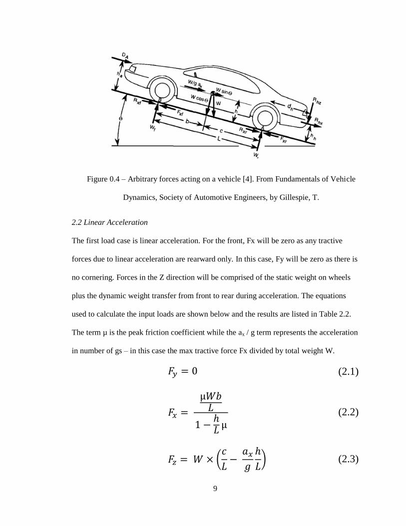
9
Figure 0.4 – Arbitrary forces acting on a vehicle [4]. From Fundamentals of Vehicle
Dynamics, Society of Automotive Engineers, by Gillespie, T.
2.2 Linear Acceleration
The first load case is linear acceleration. For the front, Fx will be zero as any tractive
forces due to linear acceleration are rearward only. In this case, Fy will be zero as there is
no cornering. Forces in the Z direction will be comprised of the static weight on wheels
plus the dynamic weight transfer from front to rear during acceleration. The equations
used to calculate the input loads are shown below and the results are listed in Table 2.2.
The term µ is the peak friction coefficient while the ax / g term represents the acceleration
in number of gs – in this case the max tractive force Fx divided by total weight W.
(2.1)
(2.2)
(
) (2.3)

10
Table 2.2 – Component forces based on the linear acceleration loading scenario.
2.3 Braking Performance
The second load case is linear braking performance. Fx is the braking force calculated
from brake gain, number of brakes per axle, applied pressure and wheel radius. In this
case, Fy will be zero as there is no cornering. The force in the Z direction is due to the
static weight on wheels plus the dynamic weight transfer. The maximum brake force is
dependent on the linear deceleration (Dx) which varies at each axle. The linear
deceleration (Dx) of the vehicle is a function of the maximum braking force on the front
axle (Fxmf), the brake force on the rear axle (Fxr) and the vehicle weight (W):
(2.4)
The maximum front axle brake force (Fxmf) can be rewritten by combining equations
(2.4) and (2.8) on pg. 13 while considering the peak coefficient of friction (μp):
(2.5)

11
Because the maximum front axle brake force is dependent on the rear axle force present,
a balance must be achieved through brake proportioning to avoid a “lock-up” condition.
A valve is used to regulate the hydraulic brake fluid between the front and rear axles –
typically equal pressure up to a specified threshold, and thereafter a percentage of the
front pressure is applied to the rear.
The applied pressure is related to the brake force by equation (2.6):
(2.6)
where:
Fb: Brake force (lb)
r: tire rolling radius (in)
G: Brake gain (in-lb/psi)
Pa: Application pressure (psi)
The brake force (Fb) represents the braking force on each individual wheel – to achieve
the brake force on the rear axle (Fxr) from the previous page; one would simply use the
rear brake gain, rear application pressure and multiply by two to account for two brakes
per axle in equation (2.6).
12
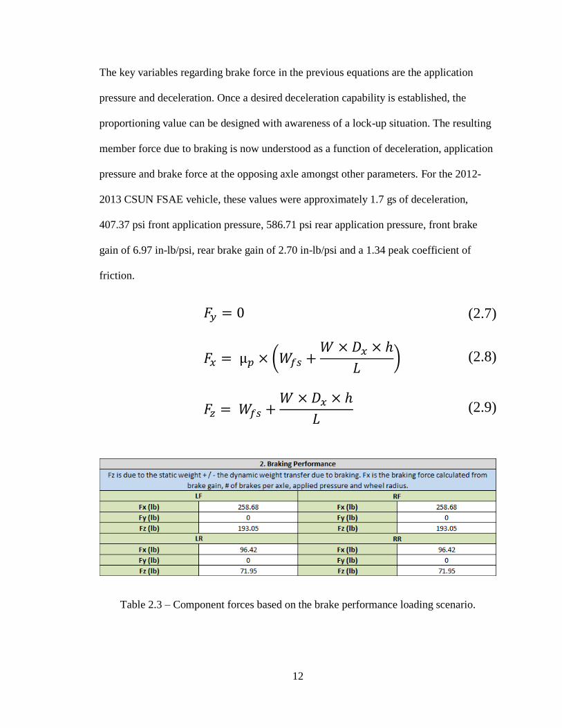
The key variables regarding brake force in the previous equations are the application
pressure and deceleration. Once a desired deceleration capability is established, the
proportioning value can be designed with awareness of a lock-up situation. The resulting
member force due to braking is now understood as a function of deceleration, application
pressure and brake force at the opposing axle amongst other parameters. For the 2012-
2013 CSUN FSAE vehicle, these values were approximately 1.7 gs of deceleration,
407.37 psi front application pressure, 586.71 psi rear application pressure, front brake
gain of 6.97 in-lb/psi, rear brake gain of 2.70 in-lb/psi and a 1.34 peak coefficient of
friction.
(2.7)
(
)
(2.8)
(2.9)
Table 2.3 – Component forces based on the brake performance loading scenario.

13
2.4 Steady State Cornering
The third load case is steady state cornering at 1.0g. Steady state means no increase or
decrease in acceleration or braking, so the forces in the X direction are zero. The forces in
the Y direction are based on the lateral acceleration as a function of the forces of the
forces in the Z direction. Because the acceleration is 1.0g in this example, the forces in Y
and Z directions are equivalent.
During cornering, the weight naturally wants to “roll” or transfer from the outside to the
inside wheel, which creates a moment with respect to the origin. On the other hand, the
suspension will resist this moment through the various components designed to counter-
act the motion: springs, anti-roll bar, etc., hence the term roll stiffness. The Kϕf and Kϕr
terms represent the roll stiffness of the suspension for the front and rear respectively and
their definitions can be found in equation (2.18). A relationship is established between
wheel loads Fz at the outside (o) and inside (i) wheels respectively, the lateral force Fy
and roll angle as shown in equation (2.10):
⁄
⁄ (2.10)
where the roll angle ϕ is defined as:
⁄
(2.11)

14
Many of the terms in these equations are based on vehicle design geometry, such as the
track width (t), roll center height (h), vehicle weight (W) and sprung mass center of
gravity above the roll axis (h1). The (V2 / Rg) term is the velocity of the vehicle, radius of
the turn and gravitational constant g – simply put this is the number of gs (equal to 1.0 for
this case) the vehicle undergoes while cornering.
Typically the cornering number of gs is an input parameter – e.g. it is desired that the
FSAE car can successfully navigate a skid pad at 1g. It is important to recognize that the
Fy term in equation (2.10) on the previous page is simply the lateral force generated by
navigating a vehicle with dynamic front weight (Wf) through a turn with radius (R) at a
velocity (V):
(2.12)
Equations (2.10), (2.11) and (2.12) can now be combined to solve for the force delta in
the Z direction. The force Fz is then multiplied by the front track width (tf) acting as a
moment arm to form the front roll moment (Mʹϕf):
⁄
⁄ (2.13)
The (h1) term is defined as the height of sprung mass center of gravity above the roll axis
[4] which for this vehicle was 12 inches. Similarly, the distance between the front axle
and the roll axis is the (hf) term at 3.03 inches. The front and rear suspension roll stiffness
values (Kϕf and Kϕr) were given by the kinetics engineer as 3219 in-lb/deg and 3663 in-
lb/deg respectively.

15
The roll moment accounts for the dynamic weight transfer due to cornering and is
explored further in section 2.5 Linear Acceleration with Cornering. The force in the Z
direction is now calculated as plus or minus the roll moment divided by the track width
plus the static weight on the front wheels.
(2.14)
(2.15)
(
)
(2.16)
Table 2.4 – Component forces based on steady state right hand cornering at a value of
constant 1.0g acceleration.
2.5 Linear Acceleration with Cornering
The fourth load case is cornering combined with linear acceleration. This load case is
complex, but also the most-likely scenario to occur for a FSAE vehicle. Compared to all
previous conditions where one force direction was always zero, forces are now apparent
in all three directions in the rear section of the vehicle. Force Fx is due to the tractive
forces generated by acceleration, calculated in the same manner as before. However,

16
because the tractive forces are based on the weight, this value will be significantly
different. When the vehicle undergoes cornering with acceleration, weight transfer occurs
not only from front to rear but from side to side as well.
Figure 0.5 – Force analysis of a simple vehicle in cornering [4]. From Fundamentals
of Vehicle Dynamics, Society of Automotive Engineers, by Gillespie, T.
The force in the Y direction is due to the centripetal force – a force that makes a body
follow a curved path. The magnitude of the centripetal force on an object of mass m
moving at tangential speed v along a path with a radius of curvature r is:
(2.17)
In a real world track situation, the radius of the turn and velocity are variables that are
changing throughout the course. In this load case scenario, it is assumed that the velocity

17
and lateral acceleration are held constant and the radius of the turn is calculated using the
above equation. If these values were always changing, it would be difficult to have one
calculated value for the amount of force generated. Because this research focuses on
optimization, the maximum values of lateral acceleration and velocity were used based
on data acquisition from previous FSAE cars.
The question then arises, if the velocity is held constant then the acceleration must be
equal to zero, but how can that be the case for cornering with linear acceleration? It is
important to note two things: the linear acceleration “term” still attributes to weight
transfer (present in all force direction equations) and that the maximum velocity and
lateral force values are used which is a valid use for optimization. The roll stiffness of the
suspension (Kϕf) is the roll resisting moment caused by the lateral separation between the
springs and is defined as follows:
(2.18)
where:
Kϕ: Roll stiffness of the suspension (lb·in/deg)
Ks: Vertical rate of each of the left and right springs (lb/in)
s: Lateral separation between the springs (in)
The spring rate is defined as the amount of weight required to deflect a spring one inch,
thus a higher value of spring rate deflects less under load – a greater resistance to vehicle
roll. Because the roll stiffness is in the numerator as shown by the roll moment equation

18
(2.13), it would seem that as the spring rate increases so does the amount of roll moment.
However, the numerator term is divided by the summation of the vehicle roll stiffness
(front and rear), thus logically reducing the amount of body roll as spring rate is
increased.
The force in the Z direction Fz is calculated from the roll moment, shown by equation
(2.19):
(2.19)
where:
⁄ ( ⁄ ) (2.20)
h1: height from roll axis to CG of vehicle (in.)
hf: roll center height with respect to front axle (in.)
tf: front track width (in.)
Kϕf, r: roll stiffness of the suspension front / rear (lb·in / deg)
These two equations show that the force in the Z direction is a function of vehicle weight,
roll axis height, track width, the roll stiffness of the suspension, velocity of the car and
radius of the turn. The first term in the roll moment equation has the Kφ term
representing the suspension resistance to the generated body roll. This roll resistance can
be varied by changing the spring rates, anti-roll bar sizing and other suspension
geometry. It is worth noting that the track width has a direct input on how much weight

19
will transfer laterally – a long track width means less transfer while a short track width
means more transfer. Body roll can be advantageous, so it should not be the objective to
rid the vehicle of all body roll, but that discussion is beyond the scope of this report.
The second term in the roll moment equation is based on the centripetal force that was
defined in equation (2.17). Although the forces in the Z direction oppose each other in a
force balance, the forces in the Y direction react in the same direction for both the inside
and outside tires. These reaction forces sum to Fy acting at the center of gravity. A
moment is generated with the moment arm as the height of the center of gravity (hf).
The roll moment equation is equal to the total change in Fz multiplied by the track width
of the vehicle. The total change in Fz is then split between the outside and inside tires
respectively. The force on the outside tire will equal the roll moment plus the weight on
the front tires divided by two. For the inside tire, the force will equal the negative roll
moment minus the weight on the front tires divided by two.

20
The calculations in Table 2.5 confirm the equations, showing that for a right hand corner
the inside tire (right hand side) reduces in magnitude while the outside tire (left hand
side) increases in magnitude with respect to a non-cornering state. Recall that in the local
coordinate system designation Fz was defined as positive downward.
The input parameters such as the suspension roll stiffness, roll center height, and roll axis
height are the same as defined in Section 2.4 Steady State Cornering. Recall that the
tractive force (Fx) is the weight on wheel (static plus or minus dynamic depending on
inside or outside wheel) multiplied by the traction limited coefficient of friction, a value
of 1.25 in this example. That is to say, Fx is 1.25 times Fz for this linear acceleration with
cornering load case.
Table 2.5 – Component forces based on right hand cornering with linear acceleration.

21
2.6 Braking with Cornering
The braking with cornering load scenario is similar to the previous linear acceleration
with cornering; however the front of the vehicle now experiences a force in the X
direction. In Table 2.5, the weight and forces are clearly shifting from the right to the left
of the vehicle which is what would be expected during right-hand cornering. In Table 2.6
the same type of weight transfer occurs, but now the transfer of rear to front caused by
braking has been added. Combine both of these weight transfers and one would expect
the left front to be the worst case for braking with right-hand cornering. Clearly in Table
2.6 the left front of the vehicle is undergoing the highest magnitude of force in all
directions.
Table 2.6 – Component forces based on right hand cornering with braking.
In this analysis only the front of the vehicle will be used, however all load cases will be
considered. The model will be setup as a one quarter vehicle, with the force magnitudes
applied regardless of left or right application. This is accomplished by default with the
geometry being symmetrical and the moment arms being the same length. In this case,
the “right-hand” geometry is used, but with the greater left-hand force magnitudes
applied.

22
2.7 5g Bump
The sixth and final load case is a 5g bump. This is an extreme scenario that is not likely
to be experienced during normal track time; however it is worth exploring to determine
the maximum loading that the suspension members can withstand. Because this condition
is already taking into account a “worse-case” situation it is treated as a static state with no
acceleration or braking as shown in Table 2.7. The magnitude of the force is simply the
mass of that vehicle corner multiplied by the acceleration – 5 times g.
Table 2.7 – Component forces based on a 5g bump condition.

23
1. CHAPTER 3 – HAND CALCULATIONS
3.1 Outline of Method
Now that the load scenarios have been established, the focus will shift to calculating the
reaction to these forces in the suspension members. In general a FSAE vehicle suspension
is comprised of six different members: a tie rod, lower control arm, upper control arm
and push (or pull) rod. There are benefits to each type of rod; however it is irrelevant for
this type of analysis. The vehicle used for these calculations utilizes push rod suspension
geometry. This member connects the front knuckle to the bell housing – a mechanism
that rotates about a fixed point on the frame and translates forces into the spring damper
assembly. The tie rod connects the knuckle to the steering gearbox assembly and
translates the linear motion of the gearbox into left / right rotation of the knuckle.
The lower and upper control arms connect the knuckle to the frame of the vehicle and are
typically comprised of two members in an “A” shape as shown in Figure 3.1. These arms
control the camber angle of the wheel and tire assembly.
Camber is described as the measure in degrees of the difference between the wheels
vertical alignment perpendicular to the surface. Basically, if the top of the tire is closer to
the frame (relative to the 0° datum) then it is said to have negative camber, whereas if it
is further away from the frame then is it said to have positive camber. A short upper
control arm combined with a long lower control arm will yield negative camber, while
positive camber is achieved by the opposite configuration. These dimensions are
determined based on what dynamic suspension characteristics are desired.

24
Figure 1.1 – Typical suspension geometry of a FSAE vehicle (front, RH side shown).
To explore the equations and matrices involved in these hand calculations, it is necessary
to define a naming convention for each of the suspension members as follows:
TR – Tie Rod
LCAF – Lower Control Arm Front
LCAR – Lower Control Arm Rear
UCAF – Upper Control Arm Front
UCAR – Upper Control Arm Rear
PR – Push Rod
25
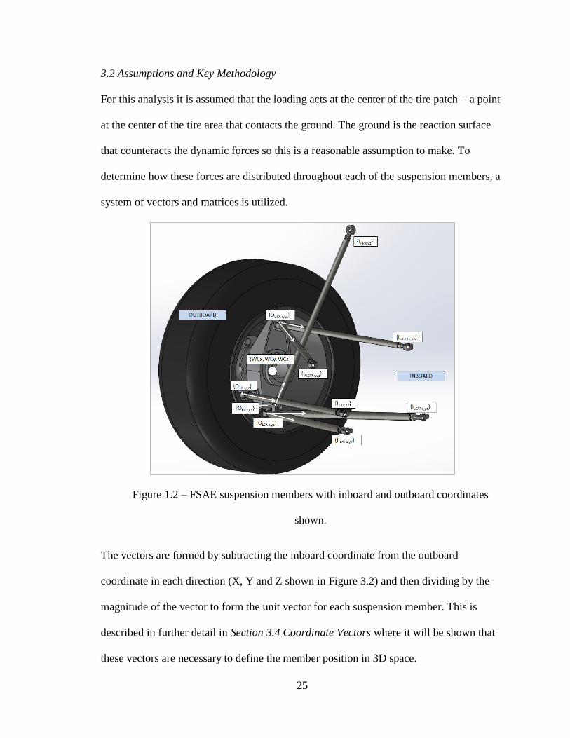
3.2 Assumptions and Key Methodology
For this analysis it is assumed that the loading acts at the center of the tire patch – a point
at the center of the tire area that contacts the ground. The ground is the reaction surface
that counteracts the dynamic forces so this is a reasonable assumption to make. To
determine how these forces are distributed throughout each of the suspension members, a
system of vectors and matrices is utilized.
Figure 1.2 – FSAE suspension members with inboard and outboard coordinates
shown.
The vectors are formed by subtracting the inboard coordinate from the outboard
coordinate in each direction (X, Y and Z shown in Figure 3.2) and then dividing by the
magnitude of the vector to form the unit vector for each suspension member. This is
described in further detail in Section 3.4 Coordinate Vectors where it will be shown that
these vectors are necessary to define the member position in 3D space.
26
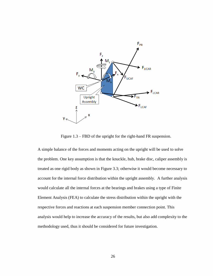
Figure 1.3 – FBD of the upright for the right-hand FR suspension.
A simple balance of the forces and moments acting on the upright will be used to solve
the problem. One key assumption is that the knuckle, hub, brake disc, caliper assembly is
treated as one rigid body as shown in Figure 3.3; otherwise it would become necessary to
account for the internal force distribution within the upright assembly. A further analysis
would calculate all the internal forces at the bearings and brakes using a type of Finite
Element Analysis (FEA) to calculate the stress distribution within the upright with the
respective forces and reactions at each suspension member connection point. This
analysis would help to increase the accuracy of the results, but also add complexity to the
methodology used, thus it should be considered for future investigation.

27
Because all of the suspension members connect to the upright assembly, the rigid body
assumption allows for the simple summation of forces previously outlined. The external
forces generated by the loading scenarios act at the center of the tire patch, however they
need to be resolved about the center of the rigid body (wheel center) defined - this will be
explained further in Section 3.4 Coordinate Vectors and Section 3.7 Formation of
Matrices.
3.3 Configuration of Equations
There are a total of six suspension members (two members for the LCA, two members
for the UCA, one tie rod and one push rod). The tension or compression forces in these
members are the six unknowns to be solved. A force and moment balance in the X, Y and
Z directions can be written with respect to the forces generated at the contact patch,
resolved about the wheel center. The wheel center will be the basis of the rigid body for
which all calculations are referred to as illustrated by the free body diagram (FBD) in
Figure 3.3. This balance will yield six equations and six unknowns (the force in each
member) that will be constructed into matrix format for a simplified solving technique.
The basic format is as follows:
[ ]{ } { } (3.1)
Matrix A is defined as a 6x6 matrix where the first three rows represent the summation of
the forces in each direction respectively. The last three rows are comprised of the
summation of moments in each direction. Matrix x is defined as a 6x1 matrix with a
column vector where each row and corresponding value represents the unknown force in

28
each of the suspension members. Matrix B is defined as a 6x1 matrix with a column
vector consisting of the x, y and z forces and moments generated at the center of the tire
patch resolved about the wheel center. To summarize, Matrix A is the derived equations,
Matrix x is the unknowns and Matrix B is the inputs.
3.4 Coordinate Vectors
To establish matrix A, the vectors for each suspension member must be formed from the
end point coordinates; these values are tabulated in Table 3.1. Using vectors allows for
the summation of the forces in three-dimensional space without the use of trigonometry.
The unit vector represents the direction of the unknown resultant force with respect to the
member geometry in 3-D space. The formation of these unit vectors will further prove to
be useful when evaluating the summation of the moments.
Table 3.1 – Suspension points for the right front corner of the FSAE vehicle.
The outboard coordinates represent the 3D point where the member attaches to the front
upright while the inboard coordinates represent the 3D point where the member attaches
to the frame of the vehicle. The vector OI can be compiled by simply subtracting the
inboard (I) coordinates from the outboard (O) as shown in equation (3.2). This is only
true if it assumed that the push rod goes directly through the ball joint. By design, the

29
push rod is connected as close as possible to the ball joint (lower arm connection point to
the upright) as to not exert a bending moment on the A-arm, thus the assumption made is
reasonable. The vectors are compiled for each suspension member using this technique as
shown in Table 3.2.
[ ] (3.2)
Table 3.2 – Vector formation and calculations for each of the front suspension members.
Once the vectors have been established for each member, a unit vector is formed. The
magnitude of the vector is calculated according to Equation (3.3). The unit vector is then
formed by dividing each component vector by the magnitude as shown in Equation (3.4).
√ ( ) (3.3)
[
] (3.4)

30
3.5 Summation of Forces
With the unit vectors set for each member, Matrix A can be formed. This matrix is simply
the summation of the forces and moments acting on the system. This system is treated as
static because the “dynamic” load scenarios are assumed constant. Because this is an
optimization problem it is important to note that the load scenarios are calculated at a
theoretical “maximum” state to account for the static assumption. Also, the 5g bump load
scenario has been added as an extreme case to help offset any lack of data or dynamic
condition that the vehicle may undergo.
Once a steady state condition has been established, the summation of the forces and
moments can be set to equal zero. Using the nomenclature defined previously for each of
the members, we can write:
∑
(3.5)
In equation (3.5) the FTR term is the axial loading in the tie rod member, while the other
terms in the equation follow the same sequence for the five remaining members. The Fx
term is the input force from the load scenario that the vehicle is subjected to. Because it is
unknown which of the pre-defined load scenarios will cause the “worst-case” condition
for the members, the forces will be evaluated for all load scenarios and then designed
based on the largest magnitude of resulting member force. This process will be repeated
for the forces and moments in the Y and Z directions as well. The sums of forces in the Y
and Z directions are shown in equation (3.6) and equation (3.7) respectively.

31
∑
(3.6)
∑
(3.7)

32
3.6 Summation of Moments
With three unknowns remaining, it is necessary to use the summation of moments to
finish solving all six equations. The wheel center becomes the reference point for all
calculations and for the right front tire it has coordinates as shown in Table 3.3. These
coordinates are based on the SolidWorks model of the FSAE vehicle with the origin [0, 0,
0] along the centerline of the vehicle (Y), at the front most point of the vehicle (X) and on
the ground plane common with the tire patch (Z) as illustrated in Figure 3.4.
Figure 1.4 – FSAE vehicle wheel center coordinates defined by SolidWorks model,
WCy not shown.
These coordinates are more simply explained by their relationship to common FSAE
vehicle parameters. The WCz term is simply the radius of the wheel - the measurement of
8.997” is about ~ 9” which is typical for a FSAE vehicle. The WCy term not shown in
Figure 3.4 is equated to be half of the track width. The track width is defined to be “the
measurement from tire center to tire center” [7] of two wheels on the same axle, each on
WCx
ORIGIN
[0
WCz
z
x

33
the other side of the vehicle. Although not defined in Table 2.1 – Typical FSAE vehicle
parameters, for the 2012-2013 CSUN FSAE the front track width was set at 50.8”
confirming the WCy term of roughly half that value. The last term, WCx is defined along
the wheelbase of the FSAE vehicle. Recall that the wheelbase is defined as “the
measurement from the middle of the front axle to the middle of rear axle” [7]. Although
the distance WCx is from the front most point on the vehicle to the front axle in this case,
the key point is to maintain consistency so that the member coordinates in Table 3.1 and
the wheel center are defined from the same relative coordinate system.
Wheel Center Coordinates (in.)
WCx 25.753
WCy 25.523
WCz 8.977
Table 3.3 – Wheel center points for the right front corner of the FSAE vehicle.
To form the moment arm, the xyz coordinates of the wheel center (WC) from Table 3.3
are subtracted from the outboard endpoints in Table 3.1 for each suspension member as
shown in equation (3.8) using the tie rod (TR) member as an example:
(3.8)
The moment arm is calculated for each axis direction and suspension member – the
results are displayed in Table 3.4. A brief check will confirm that these values are logical,
based on the defined coordinate system and relative member attachment to the upright.
For these calculations, the wheel center is assigned [0, 0, 0] coordinates – the basis of

34
how moment analysis about a point is performed. With z positive upward from the wheel
center, it would be expected that both upper control arms would have a positive moment
arm in that direction. All other members attach downward from the wheel center yielding
a negative moment arm in the Z direction – Table 3.4 is consistent with these
conclusions.
A perhaps more intriguing observation is the moment arm in the X direction. Of course
the tie rod is expected to be offset from the X plane in order to generate the necessary
motion for turning the wheels. Theoretically it should be possible to “lineup” the
attachment of the other members with the wheel center in the XZ plane thus eliminating
select moment arms and reducing internal member force. However, geometrical
constraints and suspension kinematics may prevent such construction and this concept is
beyond the scope of the analysis herein.
Table 3.4 – Moment arm for each of the suspension members, with respect to the center
of the wheel.
To form the moment summation equations, the cross product is taken between the
moment arm and the force magnitude. The cross product is defined as a binary operation
on two vectors in three-dimensional space that results in a vector which is perpendicular
to both and therefore normal to the plane containing them. To properly use the cross
product, the force magnitude needs to be made into a vector so that it has both magnitude
35
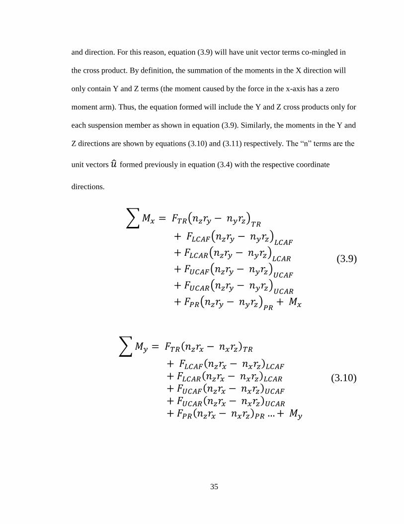
and direction. For this reason, equation (3.9) will have unit vector terms co-mingled in
the cross product. By definition, the summation of the moments in the X direction will
only contain Y and Z terms (the moment caused by the force in the x-axis has a zero
moment arm). Thus, the equation formed will include the Y and Z cross products only for
each suspension member as shown in equation (3.9). Similarly, the moments in the Y and
Z directions are shown by equations (3.10) and (3.11) respectively. The “n” terms are the
unit vectors formed previously in equation (3.4) with the respective coordinate
directions.
∑ ( )
( )
( )
( )
( )
( )
(3.9)
∑
(3.10)

36
∑ ( )
( )
( )
( )
( )
( )
(3.11)
In the above equations the forces (F) represent the unknown loading in the suspension
members. Recall that in the force summation equations (3.5 – 3.7) these unknown
member forces were also realized. Now with six equations and six equations, the solving
by matrices can begin.

37
3.7 Formation of Matrices
Recall the fundamental technique to solving the system of equations as outlined in
equation (3.12).
[ ]{ } { } (3.12)
The Matrix A has been established based on the previous sections 3.5 Summation of
Forces and 3.6 Summation of Moments. The Matrix A is of 6 x 6 form, with the first three
rows representing the summation of the forces equations (3.5 – 3.7) and the bottom three
rows the summation of the moments equations (3.9 – 3.11) as shown in equation (3.13).
[ ]
[
( ) ( )
( ) ( )
( ) ( )
( ) ( )
( ) ( )
( ) ( ) ]
(3.13)
Matrix x is of 6 x 1 form and represents the unknowns to be solved – each of the forces in
the six suspension members, shown in equation (3.14).
{ }
[
]
(3.14)

38
Matrix B is of 6 x 1 form and represents the input load cases defined in section 2.1 Input
Forces / Road Load Scenarios. Because the input load cases vary – a total of six were
outlined previously – the input values will change each time computations are made
although it is fundamentally the same as described here in equation (3.15).
[ ]
[
]
(3.15)
The moments used in Matrix B are due to the forces at the tire patch (see Figure 3.5
below) multiplied by the moment arm from the tire patch to the wheel center. These
moment arms are defined as the wheel center coordinates (WCx, WCy, and WCz from
Table 3.3) minus the coordinates at the center of the tire patch (TP). From Table 3.3, the
wheel center has coordinates of [25.753, 25.523, 8.977] and it has been established from
the SolidWorks model that the center of the tire patch has the following coordinates of
[25.753, 23.523, 0]. A simple subtraction of these coordinates forms the moment arms
shown in Table 3.5.
Moment Arm
Rx (in.) 0
Ry (in.) 0
Rz (in.) 8.997
Table 3.5 – Moment arm for center tire patch forces about the wheel center

39
In this specific example, there is no moment arm in either the X or Y axis. This means
that the center of the tire patch and wheel center are aligned except for the fundamental
difference in height (Z direction) due to the vehicle part components. This condition is
desirable and should be accounted for in the design of the suspension system. It may not
always be feasible and the drawback would be increased loading in the suspension
members (for every force there is a reaction; more forces equals more reactions).
Figure 1.5 – Forces and moments acting on a RH road wheel [4]. From Fundamentals
of Vehicle Dynamics, Society of Automotive Engineers, by Gillespie, T.
Figure 3.5 shows the moments about the tire patch, not to be confused with the moments
generated by the forces and member relative positions to the wheel center (moment arms)
in the load scenarios. The moments described here are a result of the dynamic positions
of the tire and include camber, inclination and steer (see Figure 3.6) and their effect on
the system is explored in Section 3.9 Suspension Geometry Impact.

40
Figure 1.6 – SAE tire force and moment axis system [4]. From Fundamentals of
Vehicle Dynamics, Society of Automotive Engineers, by Gillespie, T.
Figure 3.6 shows the SAE convention by which to describe the force on a tire. The three
unknown forces in matrix x are outlined in Figure 3.6 as the tractive force (Fx), lateral
force (Fy) and normal force (Fz) – the moments about wheel center are not shown here.
On front-wheel drive cars, an additional moment about the spin axis is imposed by the
drive torque. This analysis is for the front suspension of a rear-wheel drive vehicle;
however the impact of this wheel torque could easily be confirmed. A simple
investigation shows that this wheel torque acts through the wheel center; therefore no
moment is generated for the analysis of suspension members.

41
3.8 Solving of Matrices
Recall that the unknown member forces are compiled in Matrix x, thus the fundamental
equation (3.1) will be rearranged so that the unknowns can be solved for as shown in
equation (3.16).
{ } [ ][ ] (3.16)
An Excel spreadsheet has been created to quickly solve this matrix equation although any
solving technique can be applied. The suspension member force results for the braking
with right-hand cornering load scenario are shown in Table 3.6.
Matrix x
Tie Rod Force (lbf) 270.83
LCA [F] Force (lbf) 1218.87
LCA [R] Force (lbf) -1373.07
UCA [F] Force (lbf) -284.69
UCA [R] Force (lbf) 587.99
Push Rod Force (lbf) -283.79
Matrix B
Fx (lbf) 367.87
Fy (lbf) 274.53
Fz (lbf) 274.53
Mx (in- lbf) -2469.95
My (in- lbf) 3309.73
Mz (in- lbf) 0
Table 3.6 – Determination of member forces in the suspension for the braking with right-
hand cornering load case

42
For this case, Matrix B is identical to the values in Table 2.6 where the load scenario was
defined. The left hand side forces were used because they are of greater magnitude. This
analysis used the right hand geometry and the suspension geometry is symmetric about
both sides – thus the worst case situation was applied. These two matrices (x and B) are
the only ones that will change for the iteration – Matrix A by definition is comprised of
the member geometry as a unit vector (forces) along with the cross product between that
unit vector and corresponding moment arm (moments). The suspension geometry in 3-D
space will be assumed fixed for this analysis with no articulation. The results for the five
remaining load scenarios can be found in Appendix A-1.
43
3.9 Suspension Geometry Impact
A total of twenty plots were constructed based on five main scenarios:
1. Member forces vs. vertical gs
2. Member forces vs. scrub radius
3. Member forces vs. kingpin inclination angle (0 to 10 degrees)
4. Member forces vs. caster angle (0 to 10 degrees)
5. Member forces vs. caster angle vs. kingpin inclination angle (3D plot)
Each of the five plots was then repeated to produce a total of twenty plots, for the
following situations:
1. 1g vertical, lateral gs vary from 0 to 1
2. 1g vertical, longitudinal gs vary from 0 to 1
3. Vertical gs vary from 1 to 2, lateral from 0 to 1 and longitudinal from 0 to 1
These plots consider the vehicle parameters such as scrub radius, kingpin inclination
angle and caster while simultaneously subjecting the vehicle to a variety of loading
conditions. From these plots, the worst case factor of safety for each member can be
determined. Before exploring the results of these calculations, it is necessary to define the
parameters used – scrub radius, kingpin inclination angle and caster angle.

44
Figure 1.7 – Steer rotation geometry at the road wheel [4]. From Fundamentals of
Vehicle Dynamics, Society of Automotive Engineers, by Gillespie, T.
The scrub radius is defined as “the distance from the center of the tire patch to the point
where it intersects with the steering axis” [7]. Figure 3.7 illustrates this as the kingpin
offset at the ground. The steering axis is more commonly known as the “kingpin
inclination axis” which is simply the rotation axis for the wheel during steering. The axis
is normally not vertical, but may be tipped outward at the bottom, producing a lateral
inclination angle in the range of 10-15 degrees for passenger cars [4]. Both the scrub
radius and kingpin inclination angle will create an offset from the tire patch center to
wheel center in the Y direction, producing a Y moment arm not realized in previous
calculations.

45
When the steer axis from the previous paragraph is inclined in the longitudinal plane, a
caster angle is formed as illustrated in Figure 3.7. Caster is defined as “the tangential
deviation of the pivot axis in the direction of the vehicle longitudinal axis with respect to
an axis vertical to the roadway” [7]. The caster angle can be used as a tuning parameter to
add stability to the vehicle, depending on the drivetrain configuration – it works to bias
the forces either forward or rearward [8]. The key point for this analysis pertains to the
moment arm that a caster angle imposes on the system. Similar to the kingpin inclination
angle, the caster angle creates an offset (and moment arm) from the tire patch center to
the wheel center, but now in the X direction.
Recall that inherently a moment arm is realized in the Z direction by the difference in
height between the wheel center and center of the tire patch where the forces are applied,
but that Y and X coordinates were shown to be in the same plane (zero moment arms).
Now with the scrub radius, kingpin inclination angle and caster angle declared, the Y and
X moment arms need to be considered and the respective analysis will be explored in the
next section.

46
3.10 Visual Basic Iteration Method
A simple analysis in Visual Basic was used to solve the problems presented in the
previous section and the code is listed in Appendix A-2. Now the procedure used to solve
the five main scenarios will be discussed; the results will be compared to the hand
calculations derived previously, and finally safety factors will be established for each of
the suspension members. It is important to note that the method of solution unchanged
from the technique defined in Section 3.7 Formation of Matrices. This further analysis
simply explores alternative input loads to those already used in Section 2.1 Input Forces
& Road Load Scenarios and considers the impact of suspension geometrical parameters
such as the scrub radius, kingpin inclination angle and caster.
3.11 Member Forces versus Vertical Acceleration
This load case is very similar to the hand calculation methods – all moment arms are the
same, but the main change point is an iteration of the forces in the Z direction. This force
is the weight on the wheel, divided by gravity from values ranging 0 to 1 as illustrated in
equation (3.17). The weight on the wheel is not always constant due to weight transfer –
front to rear during braking and laterally during cornering.
( ⁄ ) (3.17)
The next two plots show the basic 2-D case of how the member forces vary with vertical
acceleration followed by the complex 3-D worst case with all loads – vertical, lateral and
longitudinal.

47
Figure 1.8 – Member forces versus vertical gs ranging from 1 to 2.
Figure 1.9 – Member forces versus gs in all directions; vertical 1 to 2, lateral 0 to 1
and longitudinal 0 to 1.
48
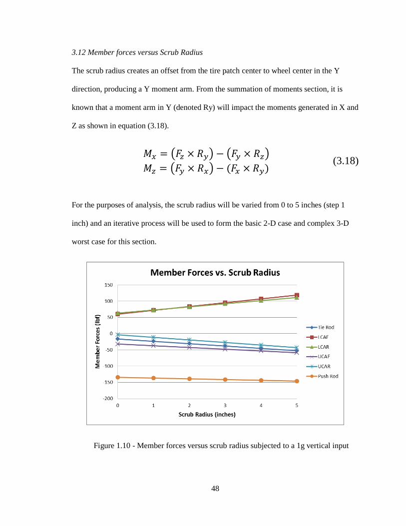
3.12 Member forces versus Scrub Radius
The scrub radius creates an offset from the tire patch center to wheel center in the Y
direction, producing a Y moment arm. From the summation of moments section, it is
known that a moment arm in Y (denoted Ry) will impact the moments generated in X and
Z as shown in equation (3.18).
( ) ( )
( ) (3.18)
For the purposes of analysis, the scrub radius will be varied from 0 to 5 inches (step 1
inch) and an iterative process will be used to form the basic 2-D case and complex 3-D
worst case for this section.
Figure 1.10 - Member forces versus scrub radius subjected to a 1g vertical input

49
Figure 1.11 – Member forces versus scrub radius; gs in all directions – vertical 1 to 2,
lateral 0 to 1 and longitudinal 0 to 1
3.13 Member forces versus Kingpin Inclination Angle
Unlike the scrub radius, the kingpin inclination angle needs to be resolved into a lateral
distance using trigonometry. The kingpin inclination angle is the angle drawn from the
center of the upper ball joint axis through the lower ball joint axis [9]. The scrub radius
accounts for the lateral offset where the kingpin axis intersects the ground plane, but not
the offset of the ball joints from the zero centerline caused by the angle. The kingpin
inclination angle is resolved into the Y component with a scrub radius of 1” as shown in
equation (3.19). The KIA (kingpin inclination angle) is varied from 0 to 10 degrees and
the respective plots are shown in Figure 3.12 and 3.13.
( ⁄ ) (3.19)

50
Figure 1.12 – Member forces versus kingpin inclination angle from 0 to 10 degrees;
scrub radius set to 1” with a 1g vertical input.
Figure 1.13 – Member forces versus kingpin inclination angle; gs in all directions –
vertical 1 to 2, lateral 0 to 1 and longitudinal 0 to 1

51
3.14 Member forces versus Caster Angle
Similar to the kingpin inclination angle, the caster angle needs to be resolved into the
correct offset distance at the ground plane through the use of trigonometry. Instead of
creating a lateral moment arm, the presence of a caster angle leads to a moment arm in
the longitudinal X direction. Caster refers to the angle made between the center of the
lower and upper pivot on the upright when viewed from the side of the vehicle and it is
illustrated in Figure 3.14. The caster angle is resolved into the X component (equation
3.20) and impacts the moments in Y and Z as shown in equation by the Rx term (3.21).
( ⁄ ) (3.20)
( ) (3.21)
Figure 1.14 – Caster angle ν resolved into x component on ground plane [4]. From
Fundamentals of Vehicle Dynamics, Society of Automotive Engineers, Gillespie, T.

52
For this analysis, the caster angle is varied from 0 to 10 degrees as described in equation
(3.20). The following plot shows the caster angle impact to the suspension members for a
1g vertical input with a zero scrub radius.
Figure 1.15 – Member forces versus caster angle from 0 to 10 degrees; scrub radius
set to 0” with a 1g vertical input
In Figure 3.15, the same parameters are used except that now that system is subjected to
input loads in all directions – vertical, lateral and longitudinal, representing the “worst-
case” scenario. Only the tie rod member is shown in this plot, although data exists for all
suspension members and it is listed in Appendix A-3.
It is important to note that although the caster angle and Rx term in equation (3.20) form
a linear relationship, this does not necessarily mean the member forces will follow that
same trend for this “worst-case” condition. This is because the caster angle impact to the
x moment arm and moment equations in equation (3.21) is only a portion of the overall

53
calculations. Figure 3.16 shows that when all inputs vary and the caster angle ranges from
0 to 10 degrees that a maximum occurs between 8 to 9 degrees for the tie rod.
Figure 1.16 – Tie rod member forces versus caster angle; input gs in all directions –
vertical 1 to 2, lateral 0 to 1 and longitudinal 0 to 1.

54
3.15 Member Forces versus Kingpin Inclination and Caster Angles
This section of the analysis combines the impact of the caster and kingpin inclination
angles. It has been shown that the caster angle creates a moment arm in the X direction
(Rx), while the kingpin inclination angle forms a moment arm in the Y direction (Ry). As
with all of these analysis cases, the moment arm in the Z direction (Rz) is caused by the
difference in height between the load application point (tire patch) and the wheel center.
Now, the effect on the suspension member loading by having a moment arm in each
direction will be realized.
(3.22)
Typically in the other scenarios, one of the moment arm terms was zero: caster angle
(Rx) with no scrub radius (Ry = 0) or kingpin inclination angle with scrub radius (both
Ry). Now, all moment arms have a magnitude and the resulting member loading due to
this is shown below in Figure 3.17.
Figure 3.18 shows part of the spreadsheet table used to form the 3-D plot. Because there
are multiple variables – vertical, lateral, and longitudinal accelerations, kingpin
inclination angle and caster angle, this analysis case will be used to determine the safety
factor for each suspension member. The data table in Figure 3.18 (full table can be found
in Appendix A-1) can be used to extract the maximum load that each member is
subjected to and the safety factor can be determined by calculating the applied versus the
allowable stress – this will be discussed in further detail in the next chapter.
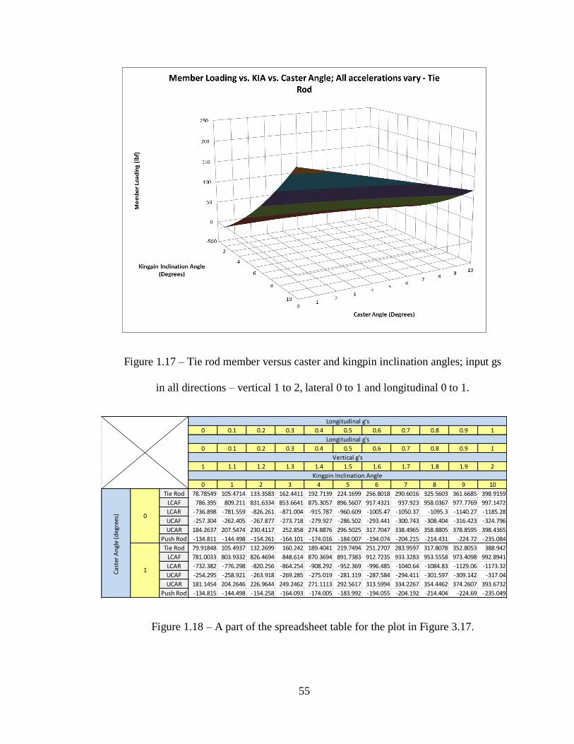
55
Figure 1.17 – Tie rod member versus caster and kingpin inclination angles; input gs
in all directions – vertical 1 to 2, lateral 0 to 1 and longitudinal 0 to 1.
Figure 1.18 – A part of the spreadsheet table for the plot in Figure 3.17.
0 0.1 0.2 0.3 0.4 0.5 0.6 0.7 0.8 0.9 1
0 0.1 0.2 0.3 0.4 0.5 0.6 0.7 0.8 0.9 1
1 1.1 1.2 1.3 1.4 1.5 1.6 1.7 1.8 1.9 2
0 1 2 3 4 5 6 7 8 9 10
Tie Rod 78.78549 105.4714 133.3583 162.4411 192.7139 224.1699 256.8018 290.6016 325.5603 361.6685 398.9159
LCAF 786.395 809.211 831.6334 853.6641 875.3057 896.5607 917.4321 937.923 958.0367 977.7769 997.1472
LCAR -736.898 -781.559 -826.261 -871.004 -915.787 -960.609 -1005.47 -1050.37 -1095.3 -1140.27 -1185.28
UCAF -257.304 -262.405 -267.877 -273.718 -279.927 -286.502 -293.441 -300.743 -308.404 -316.423 -324.796
UCAR 184.2637 207.5474 230.4117 252.858 274.8876 296.5025 317.7047 338.4965 358.8805 378.8595 398.4365
Push Rod -134.811 -144.498 -154.261 -164.101 -174.016 -184.007 -194.074 -204.215 -214.431 -224.72 -235.084
Tie Rod 79.91848 105.4937 132.2699 160.242 189.4041 219.7494 251.2707 283.9597 317.8078 352.8053 388.942
LCAF 781.0033 803.9332 826.4694 848.614 870.3694 891.7383 912.7235 933.3283 953.5558 973.4098 992.8941
LCAR -732.382 -776.298 -820.256 -864.254 -908.292 -952.369 -996.485 -1040.64 -1084.83 -1129.06 -1173.32
UCAF -254.295 -258.921 -263.918 -269.285 -275.019 -281.119 -287.584 -294.411 -301.597 -309.142 -317.04
UCAR 181.1454 204.2646 226.9644 249.2462 271.1113 292.5617 313.5994 334.2267 354.4462 374.2607 393.6732
Push Rod -134.815 -144.498 -154.258 -164.093 -174.005 -183.992 -194.055 -204.192 -214.404 -224.69 -235.049
Longitudinal g's
Kingpin Inclination Angle
Longitudinal g's
Vertical g's
0
1Cas
ter
An
gle
(deg
rees
)

56
4. CHAPTER 4 – MEMBER SPECIFICATIONS
4.1 Connection Type
The six suspension members are of tubular shape, with a hollow center and a designated
wall thickness. The connection to the frame and upright assembly is through the use of
rod end bearings (also known as heim joints) and is shown in Figure 4.1. The rod ends
are connected to the suspension members through the use of threads and a locking nut.
The purpose of these threads as opposed to a weld or other permanent method is to allow
for adjustment and initial fitment of the members. A separate study should be conducted
to confirm the strength of the connections and joints – this analysis is concentrated on the
members in regards to proper design and weight optimization.
Rod ends are primarily intended for radial loads acting in the direction of the shank axis
[1]. Although spherical bearings by design have low resistance to axial loading, they have
desirable characteristics for the movement of suspension systems. Basically the rod end
can rotate, but not translate about the coordinate axes from the center point of the
bearing. This movement is ideal for the suspension system – the desired kinematic
motion can be held while allowing some articulation about the fixed point.

57
Figure 4.1 – Spherical bearing connection of the FSAE vehicle suspension members.
The key design aspect of this connection joint is that it must allow for suspension
articulation (i.e. not fixed), yet keep the desired kinematics. This ball-and-socket joint
suppresses any linear motions and allows for only rotational degrees of freedom when
attached to a fixed point. A degree of freedom is defined as the number of independent
parameters that define its configuration. The motion is best described by successive
rotations about the three mutually perpendicular axes [2].
4.2 Boundary Conditions
The suspension members have some boundary condition at the end connections whether
it is fixed, pinned or linked to another member. For the upper and lower control arms, the
outboard members are welded together in an “A” formation to create one connection at
the upright. The tie rod has a spherical bearing heim joint, which allows for a greater
range of motion compared to the control arms. The push rod also utilizes a spherical
bearing type of connection, but notice how it does not connect directly to the upright

58
assembly. The load path for this member will have some eccentricity where the axial
force is offset from the neutral axis – more commonly known as a bending moment. The
effects of bending moments will be explored and it will become clear that this is an
undesirable attribute. All outboard connections are pictured in Figure 4.2.
Figure 4.2 – Outboard connections for the FSAE vehicle suspension members.
The tie rod and push rod allow for rotation and limited translation about the center point
of the bearing. The suspension is free to articulate except for in the direction of the
member axis, hence the loading is only axial. The exception for the push rod is the
eccentricity based on the mounting location to the lower control arm mentioned
previously. Because the lower control arms are welded together with an “A” shape, the
front and rear lower control arm members are not independent of one another and the

59
rotation is restricted. The same is true for the upper control arm members that share
similar construction. This leads to increased reactions by these members and generally a
more complex loading than pure axial.
The upright as a rigid body central connecting point for these suspension members is
subjected to forces and moments in all axis directions. The members will react to these
forces based on how they are connected to the upright assembly. If both rotation and
translation are allowed then the member will not undergo any loading (free condition). If
only translation is allowed, then the member will not react to any forces – only the
moments. Likewise if only rotation is allowed, then the member will not react to any
moments – only the forces. When the boundary condition is limited to rotation and only
forces are reacted, this becomes the desired condition because generally it is simpler to
counteract axial loading versus bending moments.
Boundary Conditions
Points Translation Rotation
Inboard Suspension Fixed Free
Outboard Suspension Z-direction Only; Fixed Free
Table 4.1 – Inboard and outboard boundary conditions for the FSAE vehicle suspension
members
A brief summary of the boundary conditions is presented in Table 4.1. The end
connections can be thought of as pinned supports – resisting vertical and horizontal
forces but not a moment. A pinned connection will allow the member to rotate, but not to
translate in any direction. The use of spherical bearings allows for free rotation at the
inboard and outboard ends, which prevents bending moments in the members. Of course,
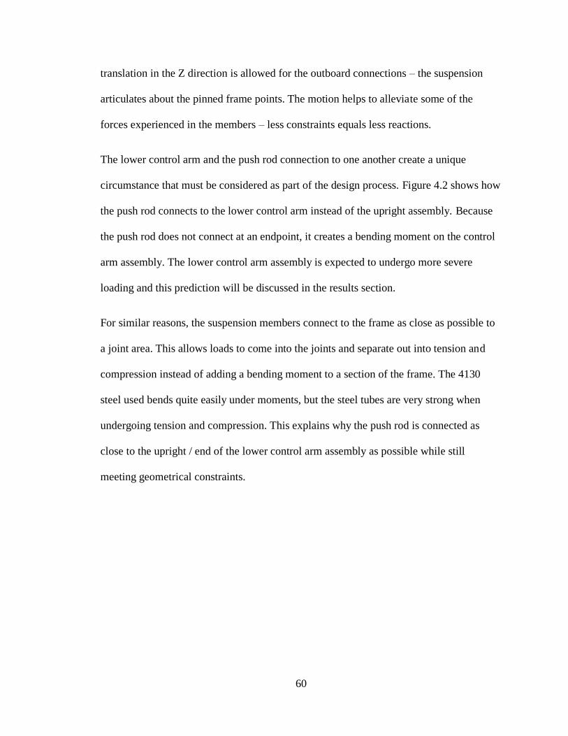
60
translation in the Z direction is allowed for the outboard connections – the suspension
articulates about the pinned frame points. The motion helps to alleviate some of the
forces experienced in the members – less constraints equals less reactions.
The lower control arm and the push rod connection to one another create a unique
circumstance that must be considered as part of the design process. Figure 4.2 shows how
the push rod connects to the lower control arm instead of the upright assembly. Because
the push rod does not connect at an endpoint, it creates a bending moment on the control
arm assembly. The lower control arm assembly is expected to undergo more severe
loading and this prediction will be discussed in the results section.
For similar reasons, the suspension members connect to the frame as close as possible to
a joint area. This allows loads to come into the joints and separate out into tension and
compression instead of adding a bending moment to a section of the frame. The 4130
steel used bends quite easily under moments, but the steel tubes are very strong when
undergoing tension and compression. This explains why the push rod is connected as
close to the upright / end of the lower control arm assembly as possible while still
meeting geometrical constraints.

61
4.3 Material Properties and Geometry
The members are of circular cross section with a hollow center, creating both inside and
outside diameters. The lengths are pre-determined based on the desired suspension
kinematics. A circular cross section should be used because of the relatively high second
moment of inertia – a measure of how good a shape is at resisting bending. The equation
for the second moment of inertia of a hollow, circular cross section is shown in equation
(4.1):
(4.1)
For a hollow rectangular cross section, the equation is similar and is shown below in
equation (4.2):
(
) (4.2)
A quick review of both equations (4.1) and (4.2) show that for a hollow square cross
section (that is to say b = h) the hollow circular cross section will have a larger area
moment of inertia. A larger area moment of inertia directly correlates to a better
resistance of bending moments. Generally, two force members are subjected to axial
normal stress which is independent of the cross section shape. However, the lower
control arm can undergo a bending moment due to the attachment point of the push rod.
The above equations confirm that a circular cross section is a good choice when
designing the members amongst other reasons such as availability, commonality and cost.

62
The FSAE team makes every effort to minimize the bending moment on the lower
control arm, but finally larger diameter tubing is used on the lower control arm as a
method to protect against any bending that may occur. The dimensions of the 2012-2013
CSUN FSAE suspension for the tie rod and lower control arm are shown in Table 4.2; the
other members are shown in Table 4.3.
Table 4.2 – Member geometry for the tie rod and lower control arm
Table 4.3 – Member geometry for the push rod and upper control arm

63
Notice how the lower control arm assembly (both front and rear members) have larger
diameter tubing comparatively – this is in anticipation of the increased magnitude of
loading and complexities of the loading described in the previous section. The members
use 4130 steel – a SAE grade steel that has an excellent strength to weight ratio and
commonly found in structural tubing and frames [3]. The material properties for 4130
steel such as elastic modulus, tensile and yield strengths are listed in Table 4.4.
Table 4.4 – Member material properties

64
CHAPTER 5 – DESIGN OF THE SUSPENSION MEMBERS
5.1 Design Criteria
The suspension members will undergo tension and compression forces, therefore both the
buckling and yield strengths need to be examined. The critical load for buckling is given
by equation (5.1):
(5.1)
where:
Pcr: Critical load (lb)
E: Elastic modulus (psi)
I: Area moment of inertia (in4)
k: Column effective length factor (k = 1.0 for pinned)
l: Unsupported length of column (in)
The elastic modulus (E), column effective length factor (k) and unsupported length of the
column (l) are fixed values. The elastic modulus is based on the material selected and its
respective properties. The column effective length factor is due to the end conditions,
which have been established in the previous section as being pinned on each end
(spherical bearing). The unsupported length of the column is determined by the desired
suspension kinematics – this value is known prior to member sizing. The design of
suspension members then becomes a function of the loading and the area moment of
inertia. A summary of the critical load values – the maximum load allowed prior to
buckling as determined by equation (5.1) – is shown in Table 5.1.

65
Tie Rod LCA [F] LCA [R] UCA [F] UCA [R] Push Rod
1926 3455 3455 2494 2861 1250
Table 5.1 – Critical loads (lbf) determined by Euler’s buckling
At this point it becomes necessary to discuss the eccentricity for the push rod that will
cause a bending condition in addition to the axial loading. The eccentricity is defined as
the force (F) being applied a distance (e) from the central axis of the member. Because
the push rod does not connect directly to the upright assembly, a moment is generated. It
is desired to eliminate this bending condition, but it is usually not possible to do so
because of geometric constraints. The distance (e) will be defined as the center of the
lower control arm spherical bearing to the push rod connection on the arm. Now that the
member will undergo a bending moment, equation (5.2) must be defined as such:
(5.2)
Equation (5.2) shows that the stress at mid-span for the member is now a combination of
the axial loading and bending moment. The (c) term is the distance from the neutral axis
to the outermost fiber of the member. Note that the bending moment, M, is negative for a
positive amount of deflection perpendicular to the center of the member, which leads to
an addition of the two terms. With the loading fixed as an input, this equation shows that
an increased cross-sectional area and area moment of inertia will reduce the amount of
stress in the member. This logic is true for the other suspension members and
optimization of the design will be considered in the results section.

66
Equation (5.1) accounts for compression (buckling) in the members, but tension
(yielding) must also be considered. Both of these failure modes will need to be
considered when establishing design criteria for the suspension members. The maximum
allowable load against tensile forces is a function of the material yield strength and the
cross-sectional area of the member. The yield strength is a fixed value based on the
material selection, thus the maximum allowable force becomes a function of the cross-
sectional area of the member; this is shown in equation (5.3).
(5.3)
A summary of the yield strength calculations – the values of maximum load allowed prior
to failure as determined by equation (5.3) – is shown in Table 5.2.
Tie Rod LCA [F] LCA [R] UCA [F] UCA [R] Push Rod
3411 4328 4328 3411 3411 2770
Table 5.2 – Maximum allowable tensile force (pound force lbf) based on yield strength
5.2 Resultant Forces
An Excel spreadsheet was created with the system of matrices outlined in Chapter 3 and
resulting forces (matrix x) were calculated for each load scenario (matrix B). Recall that
matrix A is based solely on the geometry and force balance of the system and its basis is
independent of the load case. Table 5.3 shows sample results for the braking performance
load case. Similar tables were formed for the remaining scenarios; these are located in the
section Appendix A-1.
67
Table 5.3 – Member resultant forces (lbf) for braking performance
With resultant forces determined for each load case, it becomes necessary to discern
which of the six situations will be the worst-case condition, considering both tension and
compression effects in the members. A “MIN” function in Excel was used across all six
table row cells, applied to each load case for each suspension member for the negative (-)
value compression forces. Similarly, a “MAX” function in Excel was used across all six
table row cells, applied to each load case for each suspension for the positive (+) value
tension forces. Effectively this allows for the load scenarios to be reduced to only one
criterion for design purposes – once the worst-case condition has been satisfied then the
requirements have been met. The result of this tabulation for the maximum compression
and tension forces in each suspension member is displayed in Table 5.4.
Table 5.4 – Maximum resultant compression and tension forces

68
The resultant forces were also calculated for the suspension parameter scenarios – scrub
radius, kingpin inclination angle, caster, etc. Below, the twenty plots are listed followed
by tables showing the calculated member forces for each.
1. Member forces vs. vertical gs from 1 to 2 (plot #1)
2. Member forces vs. scrub radius from 0 to 5 inches (plot #2)
3. Member forces vs. kingpin inclination angle from 0 to 10 degrees (plot #3)
4. Member forces vs. caster angle from 0 to 10 degrees (plot #4)
5. Member forces vs. caster angle vs. kingpin inclination angle (plot #5)
Each of the five plots was then repeated for the following situations:
1. 1g vertical, lateral gs vary from 0 to 1 (plots #6, 7, 8, 9, 10 respectively)
2. 1g vertical, longitudinal gs vary from 0 to 1 (plots #11, 12, 13, 14, 15 respectively)
3. Vertical gs vary from 1 to 2, lateral from 0 to 1 and longitudinal from 0 to 1 (plots
#16, 17, 18, 19, 20 respectively)
Table 5.5 – Resultant forces (lbf) for each suspension member for the first five plots.
The resultant forces for the first five plots are listed in Table 5.5 – the data for the
remaining fifteen plots may be found in Appendix A-3. Based on these twenty load
cases, the maximum and minimum forces for each member can be found. To find the
“worst-case” load scenario for the suspension members, a “MAX” function in Excel was

69
used for the highest magnitude tension forces. Likewise, a “MIN” function in Excel was
used to find the largest compressive forces. In Table 5.6, the max forces are compared
between the load cases defined in Chapter 2 based on dynamic conditions and those
outlined in Chapter 3 with the impact of suspension parameters.
Table 5.6 – Comparison of results from the two overall input loading types.
The results comparison shows similar trends – the push rod is always in compression,
never in tension (hence the term “push” rod) and the lower control arm (LCA) both front
and rear members experience the highest loading. Though in most cases, the magnitude
of the force is less when the suspension parameters are considered, recall that the load
scenarios from Chapter 2 include a 5g bump – basically a theoretical worst-case that is
unlikely to occur in a real situation. It is also important to note that with the suspension
conditions some of the members undergo a larger range of force, exposing smaller
factors of safety than seen with the dynamic scenarios from Chapter 2.
5.3 Factor of Safety
From Section 4.3 Material Properties and Geometry and 5.1 Design Criteria the material
strength and limitations were established with respect to buckling and yield. Then in
Section 5.2 Resultant Forces, the resultant forces in the suspension members were
tabulated – a worst-case condition value for both the compression and tension
MemberMax Compression
Force (lbf)
Max Tension Force
(lbf)
Max Compression
Force (lbf)
Max Tension Force
(lbf)
Tie Rod -82.55 270.83 -498.87 460.53
LCA [F] -27.03 1218.87 -67.85 601.81
LCA [R] -1373.07 315.94 -664.76 126.38
UCA [F] -333.13 69.07 -275.92 138.74
UCA [R] -17.82 587.99 -47.40 312.60
Push Rod -672.43 -68.70 -273.53 -134.49
Load Scenarios from Ch.2 Loading w/suspension conditions

70
circumstances. With an allowable loading established for the member and the induced
loading determined by the calculations, a factor of safety (FoS) can be calculated as
shown in equation (5.4).
(5.4)
Using the tie rod data from Table 5.4 and critical buckling load as an example:
⁄
⁄ (5.5)
The factor of safety for each member under compression and tension has been tabulated
in Table 5.7. This table contains valuable information – the members can be judged as
meeting the design and safety requirements, but also a trend is established that can be a
logical check to what loading the members undergo.
FoS Tie Rod LCA [F] LCA [R] UCA [F] UCA [R] Push Rod
Buckling 23.34 127.84 2.52 7.49 160.59 1.86
Yielding 12.60 3.55 13.70 49.39 5.80 40.32
Table 5.7 – Factor of safety against buckling and yielding for each member (dynamic
scenarios)
In Table 5.6, the “worst-case” input forces were found for tension and compression in the
suspension members with respect to the suspension parameter impact method. The
allowable load against buckling and yielding described in the previous section combined

71
with equation (5.5) allows for the determination of the factor of safety defined below in
Table 5.8.
FoS Tie Rod LCA [F] LCA [R] UCA [F] UCA [R] Push Rod
Buckling 3.86 50.92 5.20 9.04 60.36 4.57
Yielding 7.41 7.19 34.25 24.59 10.91 20.60
Table 5.8 – Factor of safety against buckling and yielding for each member (suspension
parameters impact)
In no particular order, here are some of the key points:
The lower control arms (LCA) and push rod (PR) have the lowest overall factor of
safety – they undergo more loading than the other members.
Based on the factor of safety, it becomes apparent which members experience
what type of loading.
Clearly the front lower control arm (LCAF), and rear upper control arm (UCAR)
are in tension while the rear lower control arm (LCAR), front upper control arm
(UCAF), tie rod (TR), and push rod (PR) are in compression.
The high factor of safety in some cases such as the LCA [F] and UCA [R] for
buckling should not come as a surprise. Essentially these values have no meaning
as the member is not experiencing the load type that the safety factor is protecting
against.
Although a FoS against yielding is listed for the push rod, this is because the
absolute value was used – technically the FoS is infinity as the push rod never
undergoes tension (max force was a compression of -134.49 lbf). It potentially
could yield in compression, but the numbers show buckling would occur first.
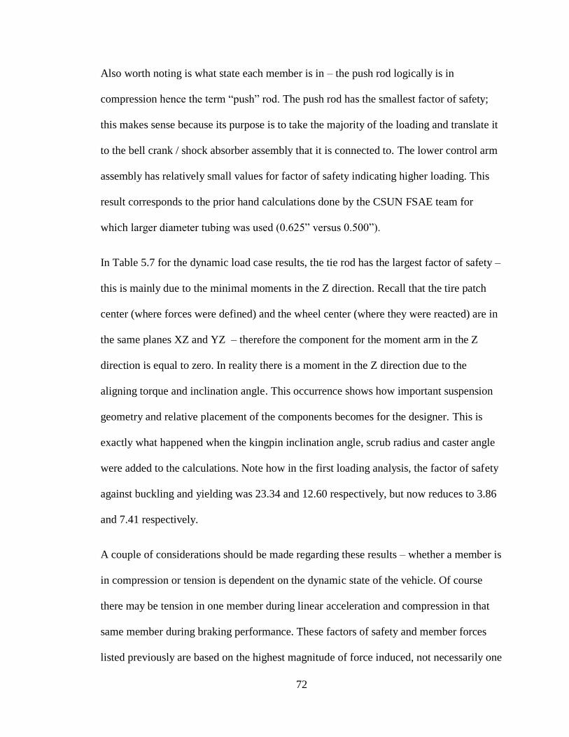
72
Also worth noting is what state each member is in – the push rod logically is in
compression hence the term “push” rod. The push rod has the smallest factor of safety;
this makes sense because its purpose is to take the majority of the loading and translate it
to the bell crank / shock absorber assembly that it is connected to. The lower control arm
assembly has relatively small values for factor of safety indicating higher loading. This
result corresponds to the prior hand calculations done by the CSUN FSAE team for
which larger diameter tubing was used (0.625” versus 0.500”).
In Table 5.7 for the dynamic load case results, the tie rod has the largest factor of safety –
this is mainly due to the minimal moments in the Z direction. Recall that the tire patch
center (where forces were defined) and the wheel center (where they were reacted) are in
the same planes XZ and YZ – therefore the component for the moment arm in the Z
direction is equal to zero. In reality there is a moment in the Z direction due to the
aligning torque and inclination angle. This occurrence shows how important suspension
geometry and relative placement of the components becomes for the designer. This is
exactly what happened when the kingpin inclination angle, scrub radius and caster angle
were added to the calculations. Note how in the first loading analysis, the factor of safety
against buckling and yielding was 23.34 and 12.60 respectively, but now reduces to 3.86
and 7.41 respectively.
A couple of considerations should be made regarding these results – whether a member is
in compression or tension is dependent on the dynamic state of the vehicle. Of course
there may be tension in one member during linear acceleration and compression in that
same member during braking performance. These factors of safety and member forces
listed previously are based on the highest magnitude of force induced, not necessarily one

73
of the specific cases defined in Chapter 2 - Preliminary Calculations. These maximum
compressive and tensile forces are derived from almost every load case; it is highly un-
likely and not feasible that a vehicle undergo full braking, a 5g bump and cornering
simultaneously. With that being said, conservative results are needed to counteract some
of the many assumptions used to generate the model and calculations methodology.

74
5.4 Design Process
The calculation methods outlined in this thesis can be used to optimize and verify the
design of FSAE suspension members – a helpful tool that the FSAE team at CSUN will
certainly be able to use over the years. The basic steps for sizing the members are to
establish the member endpoints in space (based on desired kinematics), determine the
load scenarios the FSAE vehicle is expected to undergo, set up the matrices outlined in
Chapters 2 and 3 and then evaluate the tube diameter for a chosen factor of safety.
The equations defined in Chapter 5 can easily be arranged as follows to satisfy this
design process:
(5.6)
This equation (5.6) uses the tie rod as an example and combines equations (5.1, 5.5 and
4.1). Essentially everything on the left side of the equation is constant. A factor of safety
target can be set (typically 2.5~3), k is a function of the end conditions (pinned), the
length l is determined by kinematics, Young’s modulus is based on the material selection
and the maximum force in the tie rod was determined in this thesis. The only “variables”
left are the inner and outer radius of the member – the minimum value can be determined
based on the maximum determined loading; an optimization routine has been formed.
Future analysis should include the review of assumptions made to use this model and the
development of an iterative process in either Excel or MatLAB to deliver these results in
one streamlined process.

75
5.5 Conclusion and Recommendations
Reviewing the factors of safety for the suspension members shows that the current CSUN
FSAE design is correct in terms of the sizing, material and joint connections used. The
smallest factor of safety in this analysis for the LCA is 2.52 and 3.55 (FR and RR), with
the member consisting of a comparatively larger outer diameter of 0.625”. If the LCA
member was the same as the other members (outer diameter of 0.500”) these safety
factors would reduce to 1.23 and 2.80 respectively.
By general engineering principle, it is desired that the factor of safety be at least 2.0 or
greater – that the applied loading is half of the allowable or less. However, when
referring to the suspension of a FSAE vehicle, often times an even higher factor of safety
is desired. The suspension is a vital system as without it the FSAE vehicle would not be
able to function. Furthermore, according to the 2014 FSAE rules, “Any vehicle condition
that could compromise vehicle integrity, or could compromise the track surface or could
pose a potential hazard to participants, e.g. damaged suspension … will be a valid reason
for exclusion by the official until the problem is rectified” [10].
Assuming that the factor of safety is OK if the members reduced in size the weight
benefit can be examined. Using the front LCA (LCAF) as an example, the current sizing
is 0.625” outer diameter with a 0.550” hollow inner diameter – a usable area of 0.069 in2.
Multiplied by the length of the member at 15.511”, the volume is calculated to be a value
of 1.07 in3. Now, using the 4130 steel density of 0.284 lb/in
3 [11], the weight of the
member is found to be 0.2858 lb. When these calculations are repeated for a reduced
member size (.50” outer and .43” inner diameters), the weight decreases to .2252lb,

76
creating a delta of 0.0605 lb between the larger and smaller member sizes. However, a
smaller member diameter is not the only method to reduce weight – the material may also
be changed to something more performance oriented. Carbon fiber and its high strength
to weight ratio is an ideal material from a performance standpoint and there are already
technical papers regarding its use in FSAE vehicles [13] – the use of which should not be
overlooked.
The real advantage to this process is having a clear methodology for suspension design
that can reasonably and logically predict the forces that the suspension members of a
FSAE vehicle are subjected to under a wide array of conditions. This provides confidence
of the design in a competition environment and allows for the exploration of further
improvements in the future. A strong recommendation would be the use of strain gauges
to measure the actual deformation of the members during typical dynamic events. Recall
that strain is defined as the stress divided by Young’s modulus [12]. Young’s modulus is
determined by the material used and is constant, therefore if the strain is known the stress
can be evaluated and the members designed according to the methods outlined in this
analysis.
Recall that this analysis introduced the “worst-case” conditions that may never be
realized in a typical FSAE dynamic event (acceleration, skid pad, autocross, etc.), hence
the importance of data acquisition for comparison. Many of the safety factors have an
opportunity for reduction (assuming a design standard of 2.0 minimum). A safety factor
by nature is just that – a factor to account for the uncertainties that may occur; there is no
need to be far above the minimum – to do so would create a redundancy taking away
from an optimal design.

77
REFERENCES
1. “Rod Ends”. http://www.skf.com/group/products.
SKF Group. Web. October 2013.
2. Hartenberg, Richard S.; Denavi, Jacques (1964). Kinematic Synthesis of Linkages.
New York: McGraw-Hill, Inc. Print.
3. “Best Practices for TIG Welding of 4310 Chrome-Moly Tubing in General
Motorsports and Aerospace Applications”.
http://www.millerwelds.com/resources/articles/Best-Practices-for-GTA-Welding-of-
4130-Chrome-Moly-Tubing. Web. October 2013.
4. Gillespie, D. Thomas. Fundamentals of Vehicle Dynamics. Society of Automotive
Engineers, Inc. 1992. Print.
5. “About Formula SAE Series”. http://students.sae.org/cds/formulaseries/about.htm.
SAE International. Web. Mar. 2014.
6. Jazar, N. Reza. Vehicle Dynamics: Theory and Application. Springer, 2008. Print.
7. “Terms and Definitions”. http://www.beissbarth.com/bbcms/cms.php.
Beissbarth. Web. Mar. 2014.
8. “The Caster Angle Effect”.
http://www.rctek.com/technical/handling/caster_angle_advanced.html.
RcTek. Web. Mar 2014.
9. “Suspension Theory 101”. http://www.route66hotrodhigh.com/SteeringInfo.html.
Route 66 Hot Rod High. Web. Apr 2014.
10. “Rules & Important Documents”. http://students.sae.org/cds/formulaseries/rules.
SAE International. Web. Apr 2014.
11. Central Steel & Wire Company Catalog. Typical Mechanical Properties of Standard
Carbon and Alloy Steels. (2006-2008 edition). Print.
12. “Stress, Strain and Young’s Modulus”. http://www.engineeringtoolbox.com/stress-
strain-d_950.html. The Engineering ToolBox. Web. Apr 2014.
13. Cobi, C. Alban. Design of a Carbon Fiber Suspension System for FSAE Applications.
Massachusetts Institute of Technology. June 2012. Print.

78
APPENDIX A-1
Matrix x for Linear Acceleration
Matrix x for Braking Performance
Matrix x for Steady State Cornering

79
Matrix x for Linear Acceleration with Cornering
Matrix x for Braking with Cornering
Matrix x for 5g Bump

80
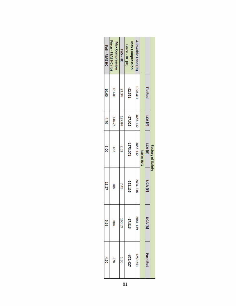
81

82
APPENDIX A-2
VBA Code Used to Generate the Plots in Chapter 3 – 3.10 through 3.15
‘Code shown for plots #1, #6 and #11 (others similar)
Sub verticalgs()
Dim matrixB As Range
Dim matrixB2 As Range
Dim matrixB3 As Range
Dim matrixA As Range
Dim matrixX As Range
Dim matrixX2 As Range
Dim matrixX3 As Range
'For vertical g case
For i = 1 To 2 Step 0.2
Sheets("Tire Data").Select
Wfs = Range("B8").Value
W = Range("B2").Value
h = Range("B6").Value
L = Range("B5").Value
'Fx3 = due to braking force (greater than linear acceleration in our analysis), (i-1) =
deceleration in gs from 0 to 1 step 0.2
'Fy2 = Fz* lateral gs range
'Fz2 = vertical gs constant at 1
Fx = Range("F76").Value
Fx3 = ((Wfs / 2) + ((W / 2) * h / L)) * (i - 1)
Fy = Range("F77").Value
Fy2 = Range("B42").Value * (i - 1)
Fz = (Wfs / 2) * i
Fz2 = (Wfs / 2) * 1
Sheets("Hand Calcs").Select
'Moment arms
Rx = Range("E52").Value
Ry = Range("E53").Value
Rz = Range("E54").Value
'Vertical force from 1 to 2 gs (Graph #1)

83
Range("B60").Value = Fx
Range("B61").Value = Fy
Range("B62").Value = Fz
Mx = (Fz * Ry) - (Fy * Rz)
My = (Fx * Rz) - (Fz * Rx)
Mz = (Fy * Rx) - (Fx * Ry)
Range("B63").Value = Mx
Range("B64").Value = My
Range("B65").Value = Mz
Set matrixB = Range("B60:B65")
'Repeat for lateral gs vary from 0 to 1 (Graph #6)
Range("C60").Value = Fx
Range("C61").Value = Fy2
Range("C62").Value = Fz2
Mx2 = (Fz2 * Ry) - (Fy2 * Rz)
My2 = (Fx * Rz) - (Fz2 * Rx)
Mz2 = (Fy2 * Rx) - (Fx * Ry)
Range("C63").Value = Mx2
Range("C64").Value = My2
Range("C65").Value = Mz2
Set matrixB2 = Range("C60:C65")
'Repeat for long gs vary from 0 to 1 (Graph #11)
Range("D60").Value = Fx3
Range("D61").Value = Fy
Range("D62").Value = Fz2
Mx3 = (Fz2 * Ry) - (Fy * Rz)
My3 = (Fx3 * Rz) - (Fz2 * Rx)
Mz3 = (Fy * Rx) - (Fx3 * Ry)
Range("D63").Value = Mx3
Range("D64").Value = My3
Range("D65").Value = Mz3
Set matrixB3 = Range("D60:D65")
'Matrix A (composed of member vertice coordinate pts)
Set matrixA = Range("B44:G49")
Sheets("Vertical gs").Select
counter = counter + 1
Set matrixX = Range(Cells(3, counter + 2), Cells(8, counter + 2))
Set matrixX2 = Range(Cells(11, counter + 2), Cells(16, counter + 2))
Set matrixX3 = Range(Cells(19, counter + 2), Cells(24, counter + 2))
matrixX.Value = Application.WorksheetFunction.MMult(matrixA, matrixB)

84
matrixX2.Value = Application.WorksheetFunction.MMult(matrixA, matrixB2)
matrixX3.Value = Application.WorksheetFunction.MMult(matrixA, matrixB3)
Next
End Sub
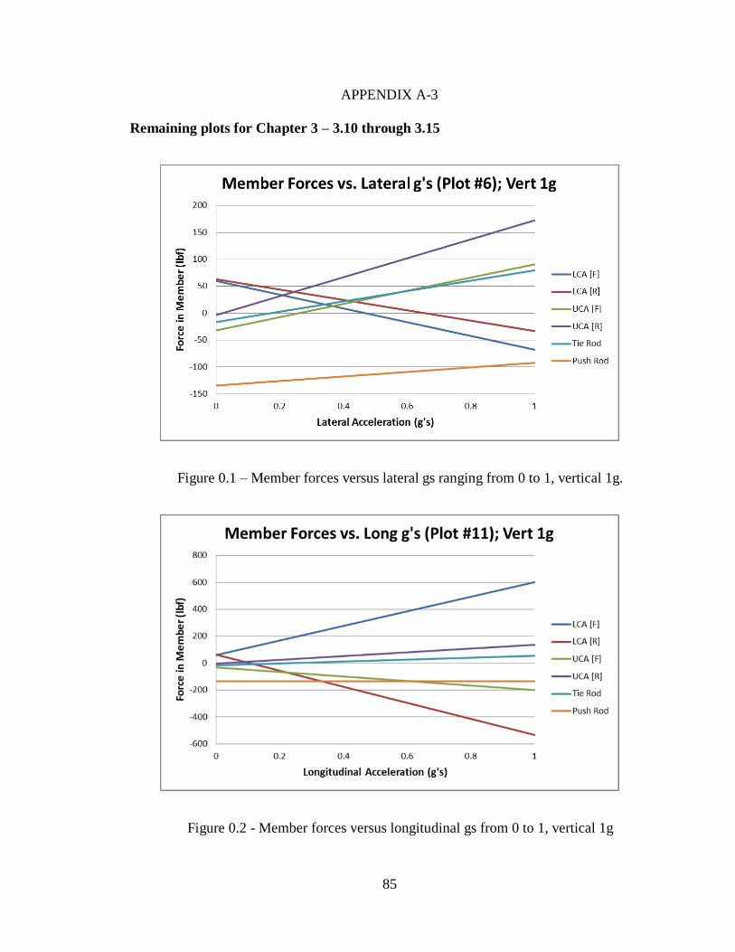
85
APPENDIX A-3
Remaining plots for Chapter 3 – 3.10 through 3.15
Figure 0.1 – Member forces versus lateral gs ranging from 0 to 1, vertical 1g.
Figure 0.2 - Member forces versus longitudinal gs from 0 to 1, vertical 1g

86
Figure 0.3 – Member forces versus scrub radius, lateral gs vary from 0 to 1, 1g
vertical.
Figure 0.4 – Member forces versus scrub radius, longitudinal gs vary from 0 to 1, 1g
vertical.

87
Figure 0.5 – Member forces versus kingpin inclination angle, 1” scrub radius, 1g
vertical, lateral gs vary from 0 to 1
Figure 0.6 – Member forces versus kingpin inclination angle, 1” scrub radius, 1g
vertical, longitudinal gs vary from 0 to 1

88
Figure 0.7 – Member forces versus caster angle, 1g vertical, lateral gs vary 0 to 1
Figure 0.8 – Member forces versus caster angle, 1g vertical, long gs vary 0 to 1

89
Figure 0.9 – Member forces versus kingpin inclination and caster angle; 1g vertical
Figure 0.10 – Member forces versus kingpin inclination angle and caster angle; 1g
vertical, lateral gs vary from 0 to 1
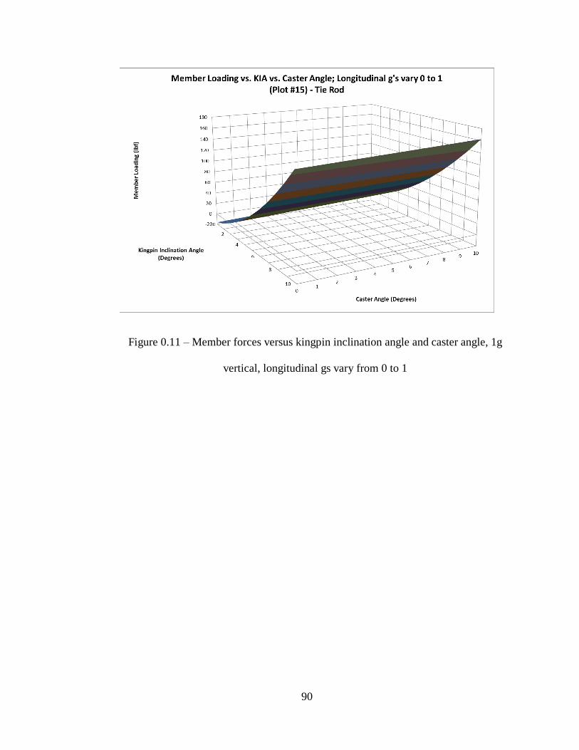
90
Figure 0.11 – Member forces versus kingpin inclination angle and caster angle, 1g
vertical, longitudinal gs vary from 0 to 1

91
1 1.2 1.4 1.6 1.8 2
-16.5103 -19.81 -23.11 -26.42 -29.72 -33.02
59.96964 71.96 83.96 95.95 107.95 119.94
63.18899 75.83 88.46 101.10 113.74 126.38
-31.9032 -38.2838 -44.6645 -51.0451 -57.4257 -63.8064
-3.5632 -4.27584 -4.98848 -5.70112 -6.41376 -7.1264
-134.485 -161.383 -188.28 -215.177 -242.074 -268.971
0 0.2 0.4 0.6 0.8 1
-16.5103 2.72833 21.96695 41.20558 60.4442 79.68282
59.96964 34.40529 8.840933 -16.7234 -42.2878 -67.8521
63.18899 43.92958 24.67018 5.410777 -13.8486 -33.108
-31.9032 -7.36517 17.17285 41.71088 66.2489 90.78692
-3.5632 31.64873 66.86066 102.0726 137.2845 172.4964
-134.485 -126.038 -117.59 -109.143 -100.695 -92.2479
0 0.2 0.4 0.6 0.8 1
-16.5103 -2.29404 11.92222 26.13848 40.35473 54.57099
59.96964 168.338 276.7064 385.0748 493.4431 601.8115
63.18899 -56.1682 -175.525 -294.883 -414.24 -533.597
-31.9032 -65.5286 -99.154 -132.779 -166.405 -200.03
-3.5632 24.45687 52.47695 80.49702 108.5171 136.5372
-134.485 -134.534 -134.583 -134.631 -134.68 -134.729
UCA [F] Force (lb)
UCA [R] Force (lb)
Push Rod Force (lb)
Vertical G's
Case # 1 - Member Forces vs. Vertical G's (vary from 1 to 2)
Tie Rod Force (lb)
LCA [F] Force (lb)
LCA [R] Force (lb)
Case # 6 - Member Forces vs. 1G Vertical (lateral gs vary from 0 to 1)
Tie Rod Force (lb)
LCA [F] Force (lb)
LCA [R] Force (lb)
UCA [F] Force (lb)
UCA [R] Force (lb)
Push Rod Force (lb)
Lateral G's
Tie Rod Force (lb)
Case # 11 - Member Forces vs. 1G Vertical (long gs vary from 0 to 1)
Longitudinal G's
LCA [F] Force (lb)
LCA [R] Force (lb)
UCA [F] Force (lb)
UCA [R] Force (lb)
Push Rod Force (lb)

92
1 1.2 1.4 1.6 1.8 2
Tie Rod -16.5103 -19.8124 -23.1144 -26.4165 -29.7185 -33.0206
LCAF 59.96964 71.96357 83.9575 95.95143 107.9454 119.9393
LCAR 63.18899 75.82678 88.46458 101.1024 113.7402 126.378
UCAF -31.9032 -38.2838 -44.6645 -51.0451 -57.4257 -63.8064
UCAR -3.5632 -4.27584 -4.98848 -5.70112 -6.41376 -7.1264
Push Rod -134.485 -161.383 -188.28 -215.177 -242.074 -268.971
Tie Rod 16.94459 13.64253 10.34047 7.038411 3.736352 0.434293
LCAF 142.7737 154.7676 166.7615 178.7554 190.7494 202.7433
LCAR -75.4276 -62.7898 -50.152 -37.5142 -24.8764 -12.2386
UCAF -40.9906 -47.3712 -53.7519 -60.1325 -66.5131 -72.8938
UCAR 59.6688 58.95616 58.24352 57.53088 56.81824 56.1056
Push Rod -126.087 -152.984 -179.881 -206.778 -233.675 -260.572
Tie Rod 50.39947 47.09741 43.79535 40.49329 37.19123 33.88917
LCAF 225.5777 237.5716 249.5655 261.5595 273.5534 285.5473
LCAR -214.044 -201.406 -188.769 -176.131 -163.493 -150.855
UCAF -50.078 -56.4586 -62.8392 -69.2199 -75.6005 -81.9812
UCAR 122.9008 122.1882 121.4755 120.7629 120.0502 119.3376
Push Rod -117.688 -144.585 -171.482 -198.379 -225.276 -252.173
Tie Rod 83.85435 80.55229 77.25023 73.94817 70.64611 67.34405
LCAF 308.3817 320.3756 332.3695 344.3635 356.3574 368.3513
LCAR -352.661 -340.023 -327.385 -314.747 -302.11 -289.472
UCAF -59.1654 -65.546 -71.9266 -78.3073 -84.6879 -91.0686
UCAR 186.1328 185.4202 184.7075 183.9949 183.2822 182.5696
Push Rod -109.289 -136.186 -163.083 -189.98 -216.877 -243.774
Tie Rod 117.3092 114.0072 110.7051 107.4031 104.101 100.7989
LCAF 391.1857 403.1796 415.1736 427.1675 439.1614 451.1553
LCAR -491.277 -478.64 -466.002 -453.364 -440.726 -428.088
UCAF -68.2528 -74.6334 -81.014 -87.3947 -93.7753 -100.156
UCAR 249.3648 248.6522 247.9395 247.2269 246.5143 245.8016
Push Rod -100.89 -127.787 -154.684 -181.581 -208.478 -235.375
Tie Rod 150.7641 147.4621 144.16 140.8579 137.5559 134.2538
LCAF 473.9897 485.9836 497.9776 509.9715 521.9654 533.9594
LCAR -629.894 -617.256 -604.618 -591.981 -579.343 -566.705
UCAF -77.3401 -83.7208 -90.1014 -96.4821 -102.863 -109.243
UCAR 312.5968 311.8842 311.1715 310.4589 309.7463 309.0336
Push Rod -92.4909 -119.388 -146.285 -173.182 -200.079 -226.976
Vertical gs
Late
ral /
Lo
ngi
tud
inal
gs
0
0.2
0.4
0.6
0.8
1

93
0 1 2 3 4 5
-16.5103 -23.7345 -30.9588 -38.183 -45.4073 -52.6315
59.96964 71.70493 83.44022 95.1755 106.9108 118.6461
63.18899 72.78059 82.37219 91.9638 101.5554 111.147
-31.9032 -37.2598 -42.6165 -47.9732 -53.3298 -58.6865
-3.5632 -11.4614 -19.3596 -27.2577 -35.1559 -43.0541
-134.485 -136.766 -139.046 -141.326 -143.607 -145.887
0 0.2 0.4 0.6 0.8 1
0 1 2 3 4 5
-16.5103 -4.49591 7.518465 19.53284 31.54722 43.5616
59.96964 46.14058 32.31151 18.48244 4.65337 -9.1757
63.18899 53.52119 43.85339 34.18559 24.51778 14.84998
-31.9032 -12.7218 6.459544 25.64091 44.82228 64.00365
-3.5632 23.75055 51.0643 78.37805 105.6918 133.0056
-134.485 -128.318 -122.151 -115.984 -109.816 -103.649
0 0.2 0.4 0.6 0.8 1
0 1 2 3 4 5
-16.5103 4.317222 52.81574 128.9853 232.8258 364.3373
59.96964 172.6918 270.6509 353.847 422.28 475.9501
63.18899 -49.8896 -169.594 -295.925 -428.881 -568.463
-31.9032 -72.8495 -117.724 -166.528 -219.26 -275.921
-3.5632 14.89331 30.01903 41.81398 50.27815 55.41153
-134.485 -136.862 -139.332 -141.898 -144.558 -147.313
Scrub Radius (in)
Case # 2 - Scrub radius from 0-5 inches vs. 1g vertical
Scrub Radius (in)
Tie Rod Force (lb)
Push Rod Force (lb)
LCA [R] Force (lb)
UCA [F] Force (lb)
UCA [R] Force (lb)
Push Rod Force (lb)
Scrub Radius (in)
Long g's (Plot #12)
Tie Rod Force (lb)
LCA [F] Force (lb)
LCA [R] Force (lb)
UCA [F] Force (lb)
UCA [R] Force (lb)
LCA [F] Force (lb)
Tie Rod Force (lb)
LCA [F] Force (lb)
LCA [R] Force (lb)
UCA [F] Force (lb)
UCA [R] Force (lb)
Push Rod Force (lb)
Lateral g's (Plot #7)

94
Scrub Rad Lat / Long 1 1.2 1.4 1.6 1.8 2
Tie Rod -16.5103 -19.8124 -23.1144 -26.4165 -29.7185 -33.0206
LCAF 59.96964 71.96357 83.9575 95.95143 107.9454 119.9393
LCAR 63.18899 75.82678 88.46458 101.1024 113.7402 126.378
UCAF -31.9032 -38.2838 -44.6645 -51.0451 -57.4257 -63.8064
UCAR -3.5632 -4.27584 -4.98848 -5.70112 -6.41376 -7.1264
Push Rod -134.485 -161.383 -188.28 -215.177 -242.074 -268.971
Tie Rod 23.55585 18.80894 14.06203 9.315123 4.568216 -0.17869
LCAF 147.1274 161.4684 175.8094 190.1504 204.4914 218.8324
LCAR -69.149 -54.5929 -40.0367 -25.4806 -10.9245 3.631621
UCAF -48.3115 -55.7635 -63.2155 -70.6674 -78.1194 -85.5714
UCAR 50.10523 47.81296 45.52068 43.22841 40.93613 38.64386
Push Rod -128.414 -155.767 -183.12 -210.474 -237.827 -265.18
Tie Rod 91.29299 85.10123 78.90948 72.71772 66.52597 60.33421
LCAF 219.5222 236.2102 252.8983 269.5863 286.2744 302.9624
LCAR -208.113 -191.638 -175.164 -158.69 -142.215 -125.741
UCAF -68.6484 -77.1717 -85.695 -94.2183 -102.742 -111.265
UCAR 100.4429 96.57098 92.69907 88.82716 84.95525 81.08333
Push Rod -122.437 -150.247 -178.056 -205.865 -233.674 -261.483
Tie Rod 186.7011 179.0645 171.4279 163.7913 156.1547 148.5181
LCAF 277.1539 296.189 315.2241 334.2592 353.2943 372.3294
LCAR -353.703 -335.31 -316.917 -298.524 -280.132 -261.739
UCAF -92.9139 -102.509 -112.103 -121.698 -131.292 -140.887
UCAR 147.4498 141.9982 136.5467 131.0951 125.6436 120.192
Push Rod -116.555 -144.821 -173.086 -201.351 -229.616 -257.882
Tie Rod 309.7803 300.6988 291.6174 282.5359 273.4545 264.373
LCAF 320.0226 341.4048 362.7869 384.1691 405.5513 426.9334
LCAR -505.919 -485.608 -465.296 -444.985 -424.674 -404.363
UCAF -121.108 -131.774 -142.44 -153.106 -163.772 -174.438
UCAR 191.1259 184.0947 177.0635 170.0323 163.0011 155.97
Push Rod -110.768 -139.489 -168.21 -196.932 -225.653 -254.374
Tie Rod 460.5305 450.0042 439.4779 428.9516 418.4253 407.8989
LCAF 348.1283 371.8575 395.5867 419.3159 443.0452 466.7744
LCAR -664.76 -642.531 -620.302 -598.072 -575.843 -553.613
UCAF -153.231 -164.968 -176.705 -188.442 -200.18 -211.917
UCAR 231.4712 222.8604 214.2495 205.6387 197.0279 188.4171
Push Rod -105.075 -134.252 -163.43 -192.607 -221.784 -250.962
2
3
4
5
Vertical gs
0
0.2
0.4
0.6
0.8
1
0
1

95
01
23
45
67
89
10
-23.7345-24.8689
-26.0029-27.1362
-28.2685-29.3994
-30.5285-31.6556
-32.7803-33.9022
-35.0211
71.7049373.5476
75.389777.23069
79.0699880.90704
82.7412984.57219
86.3991688.22165
90.03912
72.7805974.28666
75.7922677.29696
78.8002780.30175
81.8009483.29738
84.7906286.2802
87.76567
-37.2598-38.1009
-38.9418-39.7821
-40.6217-41.4602
-42.2975-43.1332
-43.9671-44.799
-45.6286
-11.4614-12.7015
-13.9413-15.1804
-16.4183-17.6547
-18.8892-20.1214
-21.351-22.5776
-23.8008
-136.766-137.124
-137.482-137.839
-138.197-138.554
-138.91-139.266
-139.621-139.975
-140.328
00.1
0.20.3
0.40.5
0.60.7
0.80.9
1
01
23
45
67
89
10
-23.7345-15.2496
-6.764261.721742
10.2087818.6972
27.1873535.67956
44.1741952.67157
61.17205
71.7049360.76542
49.8253538.88415
27.9412716.99615
6.048228-4.90306
-15.8583-26.8179
-37.7827
72.7805964.65696
56.5328648.40785
40.2814632.15324
24.0227315.88947
7.75301-0.38711
-8.53134
-37.2598-25.8319
-14.4038-2.97508
8.45436819.88484
31.316642.74988
54.1849665.62208
77.0615
-11.46144.904419
21.2705937.63753
54.0055970.37516
86.74662103.1203
119.4967135.8761
152.2588
-136.766-132.9
-129.034-125.168
-121.302-117.435
-113.568-109.7
-105.831-101.961
-98.0906
00.1
0.20.3
0.40.5
0.60.7
0.80.9
1
01
23
45
67
89
10
-23.7345-9.75678
6.39309724.71346
45.2013567.85248
92.66124119.6207
148.7227179.9576
213.3146
71.70493123.4615
174.0588223.4974
271.7784318.9038
364.8762409.6988
453.3758495.9118
537.3122
72.7805912.69148
-47.9181-109.048
-170.698-232.868
-295.557-358.762
-422.483-486.718
-551.465
-37.2598-56.05
-75.1483-94.554
-114.267-134.285
-154.608-175.235
-196.164-217.393
-238.921
-11.46140.345048
11.8904323.1754
34.2007144.96731
55.4762865.72889
75.7265285.47076
94.96332
-136.766-137.175
-137.592-138.017
-138.448-138.886
-139.331-139.783
-140.242-140.706
-141.177
Pu
sh R
od
Force
(lb)
Case
# 3 - Kin
gpin
Inclin
ation
An
gle vs. 1g ve
rtical (scrub
radiu
s = 1")
KIA
(de
gree
)
Tie R
od
Force
(lb)
LCA
[F] Force
(lb)
LCA
[R] Fo
rce (lb
)
UC
A [F] Fo
rce (lb
)
UC
A [R
] Force
(lb)
KIA
(de
gree
)
Lateral g's (P
lot #8)
Lon
g g's (Plo
t #13)
KIA
(de
gree
)
Tie R
od
Force
(lb)
LCA
[F] Force
(lb)
LCA
[R] Fo
rce (lb
)
UC
A [F] Fo
rce (lb
)
UC
A [R
] Force
(lb)
Pu
sh R
od
Force
(lb)
Pu
sh R
od
Force
(lb)
Tie R
od
Force
(lb)
LCA
[F] Force
(lb)
LCA
[R] Fo
rce (lb
)
UC
A [F] Fo
rce (lb
)
UC
A [R
] Force
(lb)

96
KIA Lat / Long 1 1.2 1.4 1.6 1.8 2
Tie Rod -23.7345 -28.4814 -33.2284 -37.9753 -42.7222 -47.4691
LCAF 71.70493 86.04592 100.3869 114.7279 129.0689 143.4099
LCAR 72.78059 87.33671 101.8928 116.4489 131.0051 145.5612
UCAF -37.2598 -44.7118 -52.1638 -59.6158 -67.0677 -74.5197
UCAR -11.4614 -13.7537 -16.0459 -18.3382 -20.6305 -22.9228
Push Rod -136.766 -164.119 -191.472 -218.825 -246.178 -273.531
Tie Rod -0.13747 -5.11125 -10.085 -15.0588 -20.0326 -25.0064
LCAF 110.6793 125.3888 140.0984 154.8079 169.5174 184.2269
LCAR 3.061777 17.91911 32.77644 47.63377 62.4911 77.34843
UCAF -43.781 -51.4012 -59.0214 -66.6416 -74.2618 -81.8819
UCAR 17.95101 15.4107 12.87039 10.33009 7.789776 5.249467
Push Rod -132.952 -160.376 -187.801 -215.226 -242.651 -270.075
Tie Rod 25.63172 20.43114 15.23057 10.02999 4.829413 -0.37116
LCAF 148.4945 163.5724 178.6504 193.7283 208.8062 223.8842
LCAR -67.1775 -52.0191 -36.8606 -21.7022 -6.54373 8.614726
UCAF -50.6102 -58.3986 -66.1869 -73.9753 -81.7637 -89.552
UCAR 47.10236 44.3141 41.52583 38.73756 35.9493 33.16103
Push Rod -129.145 -156.641 -184.138 -211.634 -239.13 -266.627
Tie Rod 53.5714 48.14416 42.71692 37.28968 31.86244 26.4352
LCAF 185.1509 200.597 216.0431 231.4893 246.9354 262.3816
LCAR -137.937 -122.478 -107.019 -91.5592 -76.0998 -60.6404
UCAF -57.747 -65.7034 -73.6599 -81.6163 -89.5727 -97.5291
UCAR 75.99329 72.95722 69.92114 66.88507 63.849 60.81292
Push Rod -125.345 -152.913 -180.481 -208.049 -235.617 -263.185
Tie Rod 83.6786 78.0249 72.37121 66.71752 61.06382 55.41013
LCAF 220.6497 236.4637 252.2777 268.0917 283.9057 299.7197
LCAR -209.217 -193.457 -177.697 -161.937 -146.177 -130.417
UCAF -65.1906 -73.3149 -81.4393 -89.5636 -97.6879 -105.812
UCAR 104.6246 101.3409 98.05726 94.77361 91.48995 88.2063
Push Rod -121.553 -149.192 -176.832 -204.471 -232.11 -259.75
Tie Rod 115.949 110.0692 104.1893 98.30942 92.42955 86.54968
LCAF 254.9929 271.1743 287.3558 303.5372 319.7186 335.9
LCAR -281.017 -264.956 -248.896 -232.836 -216.775 -200.715
UCAF -72.9401 -81.2321 -89.5242 -97.8162 -106.108 -114.4
UCAR 132.9971 129.4662 125.9353 122.4043 118.8734 115.3425
Push Rod -117.768 -145.478 -173.189 -200.9 -228.611 -256.321
Tie Rod 150.3771 144.2714 138.1657 132.06 125.9543 119.8486
LCAF 288.1831 304.7314 321.2796 337.8279 354.3762 370.9244
LCAR -353.335 -336.975 -320.614 -304.254 -287.894 -271.534
UCAF -80.9944 -89.4539 -97.9134 -106.373 -114.832 -123.292
UCAR 161.1121 157.3342 153.5564 149.7786 146.0007 142.2229
Push Rod -113.989 -141.771 -169.553 -197.335 -225.117 -252.899
Tie Rod 186.9559 180.6248 174.2937 167.9625 161.6314 155.3003
LCAF 320.2236 337.138 354.0525 370.9669 387.8813 404.7958
LCAR -426.17 -409.51 -392.851 -376.192 -359.532 -342.873
UCAF -89.3522 -97.9789 -106.606 -115.232 -123.859 -132.485
UCAR 188.9706 184.9464 180.9221 176.8978 172.8735 168.8492
Push Rod -110.217 -138.07 -165.923 -193.776 -221.63 -249.483
Tie Rod 225.6772 219.1211 212.5651 206.009 199.453 192.8969
LCAF 351.1184 368.3982 385.678 402.9579 420.2377 437.5175
LCAR -499.521 -482.563 -465.605 -448.646 -431.688 -414.73
UCAF -98.0121 -106.806 -115.599 -124.392 -133.186 -141.979
UCAR 216.5742 212.304 208.0338 203.7636 199.4934 195.2232
Push Rod -106.452 -134.376 -162.3 -190.224 -218.148 -246.072
Tie Rod 266.5314 259.751 252.9705 246.1901 239.4096 232.6292
LCAF 380.8722 398.5165 416.1609 433.8052 451.4495 469.0939
LCAR -573.386 -556.129 -538.873 -521.617 -504.361 -487.105
UCAF -106.972 -115.932 -124.892 -133.852 -142.812 -151.771
UCAR 243.9244 239.4089 234.8934 230.3779 225.8624 221.3468
Push Rod -102.693 -130.688 -158.683 -186.678 -214.673 -242.668
Tie Rod 309.5078 302.5035 295.4993 288.4951 281.4909 274.4867
LCAF 409.4904 427.4983 445.5061 463.5139 481.5217 499.5296
LCAR -647.762 -630.209 -612.655 -595.102 -577.549 -559.996
UCAF -116.231 -125.357 -134.483 -143.608 -152.734 -161.86
UCAR 271.023 266.2628 261.5026 256.7425 251.9823 247.2222
Push Rod -98.9398 -127.005 -155.071 -183.137 -211.202 -239.268
2 0.2
Vertical gs
0 0
1 0.1
3 0.3
4 0.4
5 0.5
0.6
0.7
0.8
0.9
1
6
7
8
9
10

97
01
23
45
67
89
10
-16.5103-15.3773
-14.2436-13.1086
-11.9714-10.8315
-9.68812-8.54051
-7.38797-6.22977
-5.06514
59.9696454.57795
49.1829743.78141
38.3699632.94528
27.5040122.04274
16.5580111.0463
5.50403
63.1889967.70491
72.2235976.74777
81.2802585.8238
90.3812594.95545
99.5493104.1657
108.8078
-31.9032-28.894
-25.8829-22.8682
-19.848-16.8204
-13.7835-10.7354
-7.67431-4.59811
-1.50487
-3.5632-6.68151
-9.80172-12.9257
-16.0555-19.1929
-22.3398-25.4984
-28.6705-31.8582
-35.0636
-134.485-134.489
-134.493-134.497
-134.501-134.505
-134.509-134.513
-134.517-134.521
-134.525
00.1
0.20.3
0.40.5
0.60.7
0.80.9
1
01
23
45
67
89
10
-16.5103-6.98198
0.097554.724517
6.8921276.590557
3.806921-1.47478
-9.27373-19.6123
-32.5164
59.9696442.4488
26.231511.31685
-2.29446-14.6002
-25.5964-35.2776
-43.6366-50.6646
-56.351
63.1889958.3683
54.136950.49862
47.4580345.02045
43.1919341.97936
41.3903741.43348
42.11802
-31.9032-16.4512
-0.649615.50406
32.012748.87968
66.1088183.70436
101.6711120.0142
138.7396
-3.563211.07178
25.9997141.21922
56.7292972.52927
88.61883104.998
121.6673138.6273
155.8792
-134.485-130.261
-126.029-121.788
-117.539-113.281
-109.015-104.74
-100.457-96.165
-91.8642
00.1
0.20.3
0.40.5
0.60.7
0.80.9
1
01
23
45
67
89
10
-16.5103-8.26918
-0.027388.215812
16.4610824.70912
32.9606641.21639
49.4770657.74339
66.01614
59.96964108.7621
157.5513206.334
255.1067303.8662
352.6091401.332
450.0315498.704
547.3459
63.188998.026323
-47.1336-102.288
-157.434-212.569
-267.69-322.795
-377.879-432.942
-487.978
-31.9032-45.7067
-59.5084-73.3063
-87.0988-100.884
-114.66-128.424
-142.176-155.912
-169.632
-3.56327.328526
18.2183529.10437
39.9846750.85732
61.7203872.57186
83.4097894.2321
105.0367
-134.485-134.514
-134.542-134.57
-134.598-134.626
-134.655-134.683
-134.711-134.739
-134.768
Case
# 4 - Caste
r An
gle vs. 1g ve
rtical
Tie R
od
Force
(lb)
LCA
[F] Force
(lb)
LCA
[R] Fo
rce (lb
)
UC
A [F] Fo
rce (lb
)
Pu
sh R
od
Force
(lb)
Caste
r An
gle (d
egre
e)
Caste
r An
gle (d
egre
e)
Tie R
od
Force
(lb)
LCA
[F] Force
(lb)
UC
A [R
] Force
(lb)
LCA
[R] Fo
rce (lb
)
UC
A [F] Fo
rce (lb
)
UC
A [R
] Force
(lb)
Pu
sh R
od
Force
(lb)
Lateral g's (P
lot #9)
Lon
g g's (Plo
t #14)
UC
A [F] Fo
rce (lb
)
UC
A [R
] Force
(lb)
Pu
sh R
od
Force
(lb)
Caste
r An
gle (d
egre
e)
Tie R
od
Force
(lb)
LCA
[F] Force
(lb)
LCA
[R] Fo
rce (lb
)

98
Caster Lat / Long 1 1.2 1.4 1.6 1.8 2
Tie Rod -16.5103 -19.8124 -23.1144 -26.4165 -29.7185 -33.0206
LCAF 59.96964 71.96357 83.9575 95.95143 107.9454 119.9393
LCAR 63.18899 75.82678 88.46458 101.1024 113.7402 126.378
UCAF -31.9032 -38.2838 -44.6645 -51.0451 -57.4257 -63.8064
UCAR -3.5632 -4.27584 -4.98848 -5.70112 -6.41376 -7.1264
Push Rod -134.485 -161.383 -188.28 -215.177 -242.074 -268.971
Tie Rod 0.126145 -2.94932 -6.02478 -9.10024 -12.1757 -15.2512
LCAF 96.63298 107.5486 118.4642 129.3798 140.2953 151.2109
LCAR -1.31029 12.23069 25.77168 39.31266 52.85364 66.39462
UCAF -33.2639 -39.0427 -44.8215 -50.6003 -56.3791 -62.1579
UCAR 25.08182 23.74552 22.40922 21.07292 19.73661 18.40031
Push Rod -130.286 -157.184 -184.081 -210.979 -237.877 -264.775
Tie Rod 14.31381 11.46508 8.616354 5.767627 2.918901 0.070174
LCAF 134.5999 144.4365 154.2731 164.1097 173.9462 183.7828
LCAR -65.2203 -50.7756 -36.3308 -21.8861 -7.44141 7.003311
UCAF -34.275 -39.4516 -44.6282 -49.8048 -54.9814 -60.158
UCAR 54.01979 52.05945 50.0991 48.13876 46.17841 44.21807
Push Rod -126.078 -152.976 -179.875 -206.773 -233.672 -260.571
Tie Rod 26.0489 23.42719 20.80547 18.18376 15.56204 12.94033
LCAF 173.8694 182.6257 191.382 200.1383 208.8945 217.6508
LCAR -128.537 -113.188 -97.838 -82.4885 -67.1389 -51.7894
UCAF -34.9341 -39.5077 -44.0814 -48.655 -53.2286 -57.8023
UCAR 83.24934 80.66419 78.07904 75.49389 72.90874 70.3236
Push Rod -121.861 -148.76 -175.66 -202.559 -229.459 -256.358
Tie Rod 35.32464 32.93035 30.53607 28.14178 25.74749 23.3532
LCAF 214.4423 222.1163 229.7903 237.4643 245.1382 252.8122
LCAR -191.256 -175 -158.744 -142.488 -126.232 -109.976
UCAF -35.2381 -39.2077 -43.1773 -47.1469 -51.1165 -55.0861
UCAR 112.7694 109.5584 106.3473 103.1362 99.92506 96.71397
Push Rod -117.636 -144.536 -171.436 -198.337 -225.237 -252.137
Tie Rod 42.1312 39.9649 37.79859 35.63229 33.46598 31.29968
LCAF 256.3208 262.9098 269.4989 276.0879 282.677 289.266
LCAR -253.372 -236.208 -219.043 -201.878 -184.713 -167.549
UCAF -35.1839 -38.5479 -41.912 -45.2761 -48.6401 -52.0042
UCAR 142.5795 138.7409 134.9023 131.0637 127.2252 123.3866
Push Rod -113.403 -140.304 -167.205 -194.106 -221.007 -247.908
Tie Rod 46.45569 44.51807 42.58045 40.64282 38.7052 36.76758
LCAF 299.5087 305.0095 310.5103 316.0111 321.512 327.0128
LCAR -314.88 -296.803 -278.727 -260.651 -242.575 -224.498
UCAF -34.7674 -37.5241 -40.2808 -43.0375 -45.7942 -48.5509
UCAR 172.6791 168.2111 163.7431 159.2752 154.8072 150.3392
Push Rod -109.161 -136.063 -162.964 -189.866 -216.768 -243.67
Tie Rod 48.28212 46.57402 44.86591 43.15781 41.44971 39.74161
LCAF 344.0117 348.4203 352.8288 357.2374 361.6459 366.0545
LCAR -375.771 -356.78 -337.789 -318.797 -299.806 -280.815
UCAF -33.9846 -36.1317 -38.2788 -40.4259 -42.5729 -44.72
UCAR 203.0683 197.9686 192.8689 187.7693 182.6696 177.5699
Push Rod -104.91 -131.813 -158.716 -185.618 -212.521 -239.423
Tie Rod 47.5913 46.11371 44.63611 43.15852 41.68092 40.20333
LCAF 389.8369 393.1485 396.4601 399.7717 403.0833 406.3949
LCAR -436.038 -416.128 -396.219 -376.309 -356.399 -336.489
UCAF -32.8306 -34.3654 -35.9003 -37.4352 -38.97 -40.5049
UCAR 233.7476 228.0135 222.2793 216.5452 210.8111 205.077
Push Rod -100.651 -127.555 -154.458 -181.361 -208.265 -235.168
Tie Rod 44.36082 43.11487 41.86892 40.62296 39.37701 38.13105
LCAF 436.9931 439.2023 441.4116 443.6208 445.8301 448.0394
LCAR -495.674 -474.841 -454.008 -433.174 -412.341 -391.508
UCAF -31.3001 -32.2197 -33.1394 -34.059 -34.9786 -35.8982
UCAR 264.7176 258.346 251.9743 245.6027 239.231 232.8594
Push Rod -96.3837 -123.288 -150.192 -177.096 -204 -230.904
Tie Rod 38.56492 37.5519 36.53887 35.52584 34.51281 33.49978
LCAF 485.4908 486.5916 487.6924 488.7932 489.894 490.9948
LCAR -554.668 -532.906 -511.145 -489.383 -467.622 -445.86
UCAF -29.3875 -29.6885 -29.9894 -30.2904 -30.5914 -30.8924
UCAR 295.9795 288.9668 281.9541 274.9414 267.9286 260.9159
Push Rod -92.1073 -119.012 -145.917 -172.822 -199.727 -226.632
2 0.2
Vertical gs
0 0
1 0.1
3 0.3
4 0.4
5 0.5
9 0.9
10 1
6 0.6
7 0.7
8 0.8

99
0 1 2 3 4 5 6 7 8 9 10
Tie Rod -16.5103 -17.6446 -18.7786 -19.9119 -21.0442 -22.1751 -23.3043 -24.4314 -25.5561 -26.678 -27.7968
LCAF 59.96964 61.81231 63.65442 65.4954 67.3347 69.17175 71.00601 72.8369 74.66387 76.48637 78.30383
LCAR 63.18899 64.69505 66.20066 67.70535 69.20867 70.71015 72.20934 73.70578 75.19902 76.6886 78.17407
UCAF -31.9032 -32.7443 -33.5851 -34.4255 -35.265 -36.1036 -36.9408 -37.7765 -38.6105 -39.4424 -40.272
UCAR -3.5632 -4.80337 -6.04316 -7.28219 -8.52009 -9.75648 -10.991 -12.2232 -13.4528 -14.6794 -15.9026
Push Rod -134.485 -134.844 -135.201 -135.559 -135.917 -136.274 -136.63 -136.986 -137.341 -137.695 -138.048
Tie Rod -15.3773 -16.5117 -17.6457 -18.779 -19.9112 -21.0421 -22.1713 -23.2984 -24.4231 -25.545 -26.6638
LCAF 54.57795 56.42062 58.26272 60.10371 61.94301 63.78006 65.61431 67.44521 69.27218 71.09467 72.91214
LCAR 67.70491 69.21098 70.71659 72.22128 73.72459 75.22607 76.72526 78.2217 79.71494 81.20452 82.68999
UCAF -28.894 -29.7351 -30.5759 -31.4163 -32.2558 -33.0944 -33.9316 -34.7673 -35.6013 -36.4332 -37.2628
UCAR -6.68151 -7.92168 -9.16147 -10.4005 -11.6384 -12.8748 -14.1093 -15.3415 -16.5711 -17.7977 -19.0209
Push Rod -134.489 -134.847 -135.205 -135.563 -135.92 -136.277 -136.634 -136.99 -137.345 -137.699 -138.052
Tie Rod -14.2436 -15.378 -16.512 -17.6453 -18.7776 -19.9085 -21.0376 -22.1647 -23.2894 -24.4113 -25.5302
LCAF 49.18297 51.02564 52.86774 54.70873 56.54803 58.38508 60.21934 62.05023 63.8772 65.6997 67.51716
LCAR 72.22359 73.72965 75.23526 76.73995 78.24327 79.74475 81.24394 82.74038 84.23362 85.7232 87.20867
UCAF -25.8829 -26.724 -27.5649 -28.4052 -29.2448 -30.0833 -30.9206 -31.7563 -32.5902 -33.4221 -34.2517
UCAR -9.80172 -11.0419 -12.2817 -13.5207 -14.7586 -15.995 -17.2295 -18.4617 -19.6913 -20.9179 -22.1411
Push Rod -134.493 -134.851 -135.209 -135.567 -135.924 -136.281 -136.638 -136.993 -137.348 -137.703 -138.056
Tie Rod -13.1086 -14.2429 -15.3769 -16.5102 -17.6425 -18.7734 -19.9026 -21.0297 -22.1543 -23.2763 -24.3951
LCAF 43.78141 45.62408 47.46618 49.30717 51.14647 52.98352 54.81778 56.64867 58.47564 60.29814 62.1156
LCAR 76.74777 78.25384 79.75945 81.26414 82.76745 84.26894 85.76813 87.26457 88.75781 90.24739 91.73286
UCAF -22.8682 -23.7093 -24.5502 -25.3905 -26.2301 -27.0686 -27.9058 -28.7416 -29.5755 -30.4074 -31.237
UCAR -12.9257 -14.1659 -15.4057 -16.6447 -17.8826 -19.119 -20.3535 -21.5858 -22.8154 -24.042 -25.2652
Push Rod -134.497 -134.855 -135.213 -135.571 -135.928 -136.285 -136.642 -136.997 -137.352 -137.706 -138.06
Tie Rod -11.9714 -13.1058 -14.2398 -15.3731 -16.5054 -17.6363 -18.7654 -19.8925 -21.0172 -22.1391 -23.258
LCAF 38.36996 40.21263 42.05473 43.89572 45.73502 47.57207 49.40633 51.23722 53.06419 54.88668 56.70415
LCAR 81.28025 82.78631 84.29192 85.79661 87.29993 88.80141 90.3006 91.79704 93.29028 94.77986 96.26533
UCAF -19.848 -20.6891 -21.5299 -22.3703 -23.2098 -24.0484 -24.8856 -25.7213 -26.5553 -27.3872 -28.2168
UCAR -16.0555 -17.2956 -18.5354 -19.7745 -21.0124 -22.2488 -23.4833 -24.7155 -25.9451 -27.1717 -28.3949
Push Rod -134.501 -134.859 -135.217 -135.575 -135.932 -136.289 -136.645 -137.001 -137.356 -137.71 -138.063
Tie Rod -10.8315 -11.9659 -13.0999 -14.2332 -15.3654 -16.4963 -17.6255 -18.7526 -19.8773 -20.9992 -22.118
LCAF 32.94528 34.78795 36.63006 38.47104 40.31034 42.14739 43.98165 45.81254 47.63951 49.46201 51.27947
LCAR 85.8238 87.32987 88.83547 90.34016 91.84348 93.34496 94.84415 96.34059 97.83383 99.32341 100.8089
UCAF -16.8204 -17.6615 -18.5023 -19.3426 -20.1822 -21.0207 -21.858 -22.6937 -23.5277 -24.3595 -25.1891
UCAR -19.1929 -20.433 -21.6728 -22.9119 -24.1498 -25.3861 -26.6206 -27.8529 -29.0825 -30.3091 -31.5323
Push Rod -134.505 -134.863 -135.221 -135.579 -135.936 -136.293 -136.649 -137.005 -137.36 -137.714 -138.067
Tie Rod -9.68812 -10.8225 -11.9565 -13.0898 -14.222 -15.3529 -16.4821 -17.6092 -18.7339 -19.8558 -20.9746
LCAF 27.50401 29.34668 31.18878 33.02977 34.86907 36.70612 38.54038 40.37127 42.19824 44.02074 45.8382
LCAR 90.38125 91.88731 93.39292 94.89761 96.40093 97.90241 99.4016 100.898 102.3913 103.8809 105.3663
UCAF -13.7835 -14.6246 -15.4654 -16.3058 -17.1453 -17.9839 -18.8211 -19.6568 -20.4908 -21.3227 -22.1523
UCAR -22.3398 -23.58 -24.8198 -26.0588 -27.2967 -28.5331 -29.7676 -30.9999 -32.2295 -33.4561 -34.6793
Push Rod -134.509 -134.867 -135.225 -135.582 -135.94 -136.297 -136.653 -137.009 -137.364 -137.718 -138.071
Tie Rod -8.54051 -9.67485 -10.8089 -11.9422 -13.0744 -14.2053 -15.3345 -16.4616 -17.5863 -18.7082 -19.827
LCAF 22.04274 23.88541 25.72751 27.56849 29.40779 31.24485 33.0791 34.90999 36.73697 38.55946 40.37693
LCAR 94.95545 96.46152 97.96712 99.47181 100.9751 102.4766 103.9758 105.4722 106.9655 108.4551 109.9405
UCAF -10.7354 -11.5765 -12.4174 -13.2577 -14.0973 -14.9358 -15.7731 -16.6088 -17.4427 -18.2746 -19.1042
UCAR -25.4984 -26.7386 -27.9784 -29.2174 -30.4553 -31.6917 -32.9262 -34.1584 -35.388 -36.6146 -37.8378
Push Rod -134.513 -134.871 -135.229 -135.586 -135.944 -136.301 -136.657 -137.013 -137.368 -137.722 -138.075
Tie Rod -7.38797 -8.52232 -9.65632 -10.7896 -11.9219 -13.0528 -14.182 -15.3091 -16.4337 -17.5557 -18.6745
LCAF 16.55801 18.40067 20.24278 22.08376 23.92306 25.76012 27.59437 29.42526 31.25223 33.07473 34.89219
LCAR 99.5493 101.0554 102.561 104.0657 105.569 107.0705 108.5697 110.0661 111.5593 113.0489 114.5344
UCAF -7.67431 -8.51541 -9.35625 -10.1966 -11.0361 -11.8747 -12.7119 -13.5477 -14.3816 -15.2135 -16.0431
UCAR -28.6705 -29.9107 -31.1505 -32.3895 -33.6274 -34.8638 -36.0983 -37.3305 -38.5601 -39.7867 -41.0099
Push Rod -134.517 -134.875 -135.233 -135.59 -135.948 -136.305 -136.661 -137.017 -137.372 -137.726 -138.079
Tie Rod -6.22977 -7.36411 -8.49811 -9.63142 -10.7637 -11.8946 -13.0238 -14.1509 -15.2755 -16.3975 -17.5163
LCAF 11.0463 12.88897 14.73107 16.57205 18.41135 20.24841 22.08266 23.91355 25.74053 27.56302 29.38049
LCAR 104.1657 105.6718 107.1774 108.6821 110.1854 111.6869 113.1861 114.6825 116.1758 117.6654 119.1508
UCAF -4.59811 -5.43921 -6.28005 -7.12038 -7.95995 -8.79848 -9.63574 -10.4715 -11.3054 -12.1373 -12.9669
UCAR -31.8582 -33.0984 -34.3382 -35.5772 -36.8151 -38.0515 -39.286 -40.5183 -41.7479 -42.9745 -44.1977
Push Rod -134.521 -134.879 -135.237 -135.594 -135.952 -136.309 -136.665 -137.021 -137.376 -137.73 -138.083
Tie Rod -5.06514 -6.19949 -7.33349 -8.4668 -9.59907 -10.73 -11.8591 -12.9862 -14.1109 -15.2328 -16.3517
LCAF 5.50403 7.346697 9.188802 11.02978 12.86908 14.70614 16.54039 18.37128 20.19826 22.02075 23.83822
LCAR 108.8078 110.3139 111.8195 113.3242 114.8275 116.3289 117.8281 119.3246 120.8178 122.3074 123.7929
UCAF -1.50487 -2.34596 -3.18681 -4.02714 -4.8667 -5.70523 -6.54249 -7.37822 -8.21215 -9.04404 -9.87364
UCAR -35.0636 -36.3038 -37.5436 -38.7826 -40.0205 -41.2569 -42.4914 -43.7237 -44.9533 -46.1799 -47.4031
Push Rod -134.525 -134.883 -135.241 -135.598 -135.956 -136.313 -136.669 -137.025 -137.38 -137.734 -138.087
Cas
ter
An
gle
(deg
rees
)
6
7
8
9
10
4
5
Kingpin Inclination Angle
0
1
2
3

100
0 0.1 0.2 0.3 0.4 0.5 0.6 0.7 0.8 0.9 1
0 1 2 3 4 5 6 7 8 9 10
Tie Rod -16.5103 -8.02533 0.459984 8.945987 17.43303 25.92144 34.41159 42.90381 51.39843 59.89582 68.3963
LCAF 59.96964 49.03013 38.09006 27.14887 16.20599 5.260866 -5.68706 -16.6383 -27.5936 -38.5532 -49.5179
LCAR 63.18899 55.06535 46.94126 38.81625 30.68986 22.56164 14.43113 6.29787 -1.83859 -9.97871 -18.1229
UCAF -31.9032 -20.4753 -9.04711 2.381573 13.81102 25.2415 36.67325 48.10654 59.54162 70.97874 82.41815
UCAR -3.5632 12.8026 29.16877 45.5357 61.90377 78.27334 94.6448 111.0185 127.3949 143.7743 160.157
Push Rod -134.485 -130.62 -126.754 -122.888 -119.022 -115.155 -111.287 -107.419 -103.551 -99.681 -95.8104
Tie Rod -15.3773 -8.11633 -0.85501 6.40701 13.67006 20.93449 28.20065 35.46888 42.73952 50.01292 57.28941
LCAF 54.57795 44.29146 34.00441 23.71624 13.42638 3.134281 -7.16062 -17.4589 -27.7611 -38.0677 -48.3794
LCAR 67.70491 59.87437 52.04336 44.21144 36.37814 28.54301 20.70559 12.86542 5.022049 -2.82498 -10.6761
UCAF -28.894 -17.2923 -5.69035 5.912107 17.51533 29.11958 40.72511 52.33217 63.94102 75.55192 87.16511
UCAR -6.68151 9.831618 26.34513 42.85939 59.37479 75.89169 92.41049 108.9315 125.4552 141.9819 158.512
Push Rod -134.489 -130.619 -126.749 -122.879 -119.009 -115.138 -111.266 -107.394 -103.521 -99.6472 -95.7724
Tie Rod -14.2436 -8.20739 -2.1708 3.866485 9.904803 15.9445 21.98593 28.02942 34.07533 40.12399 46.17575
LCAF 49.18297 39.5499 29.91627 20.28152 10.64508 1.006399 -8.63508 -18.2799 -27.9287 -37.5819 -47.2402
LCAR 72.22359 64.68631 57.14857 49.60992 42.06989 34.52803 26.98388 19.43698 11.88687 4.33311 -3.22477
UCAF -25.8829 -14.1074 -2.33155 9.444792 21.2219 33.00003 44.77944 56.56038 68.34311 80.12789 91.91496
UCAR -9.80172 6.85883 23.51976 40.18145 56.84426 73.50859 90.17481 106.8433 123.5144 140.1885 156.866
Push Rod -134.493 -130.619 -126.745 -122.871 -118.996 -115.121 -111.245 -107.369 -103.491 -99.6134 -95.7344
Tie Rod -13.1086 -8.29856 -3.48819 1.322862 6.134953 10.94842 15.76362 20.58089 25.40057 30.223 35.04853
LCAF 43.78141 34.80256 25.82314 16.84261 7.860386 -1.12408 -10.1113 -19.102 -28.0965 -37.0955 -46.0996
LCAR 76.74777 69.50412 62.26001 55.01499 47.76859 40.52035 33.26982 26.01655 18.76007 11.49993 4.235685
UCAF -22.8682 -10.9186 1.031357 12.98179 24.93299 36.88521 48.83871 60.79375 72.75057 84.70944 96.67061
UCAR -12.9257 3.882415 20.69095 37.50024 54.31066 71.12259 87.9364 104.7525 121.5712 138.3929 155.218
Push Rod -134.497 -130.619 -126.74 -122.862 -118.983 -115.104 -111.224 -107.343 -103.462 -99.5795 -95.6963
Tie Rod -11.9714 -8.38989 -4.808 -1.22542 2.358198 5.943197 9.529921 13.11872 16.70992 20.30388 23.90094
LCAF 38.36996 30.04652 21.72252 13.3974 5.070593 -3.25846 -11.5903 -19.9255 -28.2647 -36.6083 -44.9569
LCAR 81.28025 74.33076 67.38082 60.42995 53.47771 46.52364 39.56728 32.60817 25.64585 18.67988 11.7098
UCAF -19.848 -7.72391 4.400417 16.52526 28.65087 40.7775 52.90542 65.03487 77.1661 89.29938 101.435
UCAR -16.0555 0.90055 17.85695 34.81411 51.77241 68.73221 85.6939 102.6579 119.6244 136.594 153.567
Push Rod -134.501 -130.618 -126.736 -122.853 -118.97 -115.086 -111.202 -107.318 -103.432 -99.5456 -95.6582
Tie Rod -10.8315 -8.48145 -6.13103 -3.77993 -1.42779 0.925736 3.280985 5.638304 7.998035 10.36052 12.7261
LCAF 32.94528 25.27886 17.61188 9.943771 2.273982 -5.39805 -13.0729 -20.7511 -28.4332 -36.1198 -43.8114
LCAR 85.8238 79.16919 72.51413 65.85815 59.2008 52.54161 45.88013 39.2159 32.54847 25.87738 19.20218
UCAF -16.8204 -4.52146 7.777712 20.07739 32.37784 44.67931 56.98206 69.28635 81.59243 93.90055 106.211
UCAR -19.1929 -2.0886 15.01603 32.12143 49.22795 66.33599 83.44591 100.5581 117.6729 134.7908 151.912
Push Rod -134.505 -130.618 -126.731 -122.844 -118.957 -115.069 -111.181 -107.292 -103.402 -99.5116 -95.62
Tie Rod -9.68812 -8.57329 -7.45812 -6.34225 -5.22535 -4.10707 -2.98707 -1.86499 -0.7405 0.386743 1.517084
LCAF 27.50401 20.49662 13.48866 6.479579 -0.53118 -7.54419 -14.56 -21.5792 -28.6023 -35.6298 -42.6624
LCAR 90.38125 84.02243 77.66315 71.30296 64.94139 58.57798 52.21229 45.84384 39.4722 33.09689 26.71747
UCAF -13.7835 -1.3092 11.16534 23.64039 36.11621 48.59306 61.07118 73.55084 86.03229 98.51578 111.0016
UCAR -22.3398 -5.0869 12.16642 29.42051 46.67572 63.93244 81.19105 98.45192 115.7154 132.982 150.2519
Push Rod -134.509 -130.618 -126.727 -122.836 -118.944 -115.052 -111.159 -107.266 -103.372 -99.4775 -95.5817
Tie Rod -8.54051 -8.66547 -8.79008 -8.914 -9.03688 -9.15838 -9.27816 -9.39587 -9.51116 -9.6237 -9.73314
LCAF 22.04274 15.69679 9.350283 3.002652 -3.34666 -9.69822 -16.0526 -22.4103 -28.7719 -35.1381 -41.5092
LCAR 94.95545 88.8935 82.8311 76.76777 70.70308 64.63654 58.56772 52.49615 46.42138 40.34294 34.2604
UCAF -10.7354 1.914858 14.56542 27.21649 39.86832 52.52119 65.17533 77.83101 90.48847 103.148 115.8098
UCAR -25.4984 -8.09622 9.30634 26.70965 44.1141 61.52006 78.9279 96.33801 113.7508 131.1665 148.5857
Push Rod -134.513 -130.618 -126.722 -122.827 -118.931 -115.035 -111.138 -107.241 -103.342 -99.4433 -95.5432
Tie Rod -7.38797 -8.75804 -10.1278 -11.4968 -12.8648 -14.2314 -15.5963 -16.9591 -18.3195 -19.6771 -21.0317
LCAF 16.55801 10.87635 5.194131 -0.48921 -6.17423 -11.8615 -17.5516 -23.245 -28.9424 -34.6442 -40.351
LCAR 99.5493 93.7855 88.02124 82.25607 76.48952 70.72113 64.95046 59.17703 53.40041 47.62012 41.83572
UCAF -7.67431 5.152768 17.9801 30.80794 43.63656 56.46619 69.29711 82.12956 94.9638 107.8001 120.6387
UCAR -28.6705 -11.1185 6.433969 23.98716 41.54148 59.09731 76.65503 94.21501 111.7776 129.3433 146.9123
Push Rod -134.517 -130.617 -126.718 -122.818 -118.918 -115.017 -111.116 -107.215 -103.312 -99.4089 -95.5046
Tie Rod -6.22977 -8.85107 -11.472 -14.0923 -16.7115 -19.3293 -21.9455 -24.5595 -27.1711 -29.78 -32.3858
LCAF 11.0463 6.032198 1.017537 -3.99825 -9.01571 -14.0354 -19.0579 -24.0838 -29.1136 -34.1479 -39.1872
LCAR 104.1657 98.70156 93.23692 87.77136 82.30442 76.83565 71.36459 65.89078 60.41376 54.93309 49.44831
UCAF -4.59811 8.406604 21.41158 34.41707 47.42332 60.4306 73.43916 86.44925 99.46113 112.4751 125.4913
UCAR -31.8582 -14.1556 3.547471 21.25127 38.95621 56.66265 74.37098 92.08157 109.7948 127.511 145.2307
Push Rod -134.521 -130.617 -126.713 -122.809 -118.905 -115 -111.095 -107.189 -103.282 -99.3743 -95.4657
Tie Rod -5.06514 -8.94461 -12.8237 -16.7022 -20.5796 -24.4556 -28.3299 -32.2021 -36.0719 -39.9389 -43.8029
LCAF 5.50403 1.161189 -3.18221 -7.52674 -11.8729 -16.2214 -20.5727 -24.9273 -29.2858 -33.6488 -38.0169
LCAR 108.8078 103.6449 98.48151 93.31722 88.15156 82.98406 77.81428 72.64174 67.46601 62.28661 57.1031
UCAF -1.50487 11.67848 24.86208 38.0462 51.23108 64.41699 77.60417 90.7929 103.9834 117.176 130.3708
UCAR -35.0636 -17.2095 0.644968 18.50022 36.3566 54.21449 72.07426 89.9363 107.801 125.6687 143.5397
Push Rod -134.525 -130.617 -126.709 -122.8 -118.892 -114.982 -111.073 -107.163 -103.252 -99.3396 -95.4267
Cas
ter
An
gle
(deg
rees
)
0
1
2
3
4
5
6
7
8
9
10
Lateral g's
Kingpin Inclination Angle

101
0 0.1 0.2 0.3 0.4 0.5 0.6 0.7 0.8 0.9 1
0 1 2 3 4 5 6 7 8 9 10
Tie Rod -16.5103 -9.45029 -0.21816 11.18445 24.75459 40.48796 58.37898 78.42071 100.6049 124.9221 151.3614
LCAF 59.96964 115.417 169.7051 222.8344 274.8062 325.6223 375.2854 423.7989 471.1666 517.3933 562.4845
LCAR 63.18899 4.756365 -54.1968 -113.67 -173.664 -234.177 -295.209 -356.758 -418.823 -481.401 -544.491
UCAF -31.9032 -49.7112 -67.8273 -86.251 -104.981 -124.018 -143.359 -163.004 -182.95 -203.198 -223.743
UCAR -3.5632 9.07592 21.454 33.57166 45.42967 57.02896 68.37063 79.45593 90.28626 100.8632 111.1885
Push Rod -134.485 -134.872 -135.265 -135.665 -136.073 -136.488 -136.909 -137.337 -137.772 -138.213 -138.661
Tie Rod -15.3773 -8.3173 0.914823 12.31744 25.88757 41.62095 59.51196 79.5537 101.7379 126.0551 152.4944
LCAF 54.57795 110.0253 164.3134 217.4427 269.4145 320.2306 369.8938 418.4072 465.7749 512.0016 557.0928
LCAR 67.70491 9.272289 -49.6808 -109.154 -169.148 -229.661 -290.693 -352.242 -414.307 -476.885 -539.975
UCAF -28.894 -46.702 -64.8181 -83.2417 -101.972 -121.009 -140.35 -159.994 -179.941 -200.188 -220.734
UCAR -6.68151 5.95761 18.33569 30.45335 42.31136 53.91065 65.25232 76.33762 87.16795 97.74489 108.0701
Push Rod -134.489 -134.875 -135.269 -135.669 -136.077 -136.492 -136.913 -137.341 -137.776 -138.217 -138.664
Tie Rod -14.2436 -7.18363 2.048499 13.45111 27.02125 42.75463 60.64564 80.68737 102.8716 127.1888 153.628
LCAF 49.18297 104.6303 158.9184 212.0477 264.0195 314.8356 364.4988 413.0122 460.3799 506.6067 551.6978
LCAR 72.22359 13.79096 -45.1622 -104.636 -164.63 -225.143 -286.175 -347.724 -409.788 -472.367 -535.457
UCAF -25.8829 -43.691 -61.8071 -80.2307 -98.9612 -117.998 -137.339 -156.983 -176.93 -197.177 -217.723
UCAR -9.80172 2.8374 15.21548 27.33314 39.19115 50.79044 62.13211 73.21741 84.04774 94.62468 104.9499
Push Rod -134.493 -134.879 -135.273 -135.673 -136.081 -136.496 -136.917 -137.345 -137.78 -138.221 -138.668
Tie Rod -13.1086 -6.04857 3.183558 14.58617 28.15631 43.88968 61.7807 81.82243 104.0067 128.3238 154.7631
LCAF 43.78141 99.22874 153.5168 206.6462 258.6179 309.4341 359.0972 407.6106 454.9783 501.2051 546.2963
LCAR 76.74777 18.31515 -40.638 -100.112 -160.105 -220.619 -281.65 -343.199 -405.264 -467.843 -530.933
UCAF -22.8682 -40.6762 -58.7923 -77.216 -95.9464 -114.983 -134.324 -153.969 -173.915 -194.163 -214.708
UCAR -12.9257 -0.28662 12.09146 24.20912 36.06713 47.66642 59.00809 70.09339 80.92373 91.50066 101.8259
Push Rod -134.497 -134.883 -135.277 -135.677 -136.085 -136.499 -136.921 -137.349 -137.784 -138.225 -138.672
Tie Rod -11.9714 -4.91143 4.320695 15.72331 29.29345 45.02682 62.91784 82.95957 105.1438 129.461 155.9002
LCAF 38.36996 93.81729 148.1054 201.2347 253.2065 304.0226 353.6858 402.1992 449.5669 495.7936 540.8848
LCAR 81.28025 22.84763 -36.1055 -95.5791 -155.573 -216.086 -277.118 -338.667 -400.732 -463.31 -526.4
UCAF -19.848 -37.656 -55.7721 -74.1958 -92.9262 -111.963 -131.304 -150.948 -170.895 -191.142 -211.688
UCAR -16.0555 -3.41635 8.961727 21.07938 32.93739 44.53668 55.87836 66.96365 77.79399 88.37092 98.69618
Push Rod -134.501 -134.887 -135.28 -135.681 -136.089 -136.503 -136.925 -137.353 -137.788 -138.229 -138.676
Tie Rod -10.8315 -3.77152 5.460612 16.86323 30.43336 46.16674 64.05775 84.09949 106.2837 130.6009 157.0401
LCAF 32.94528 88.39261 142.6807 195.81 247.7818 298.598 348.2611 396.7745 444.1422 490.369 535.4601
LCAR 85.8238 27.39118 -31.5619 -91.0356 -151.029 -211.543 -272.574 -334.123 -396.188 -458.767 -521.857
UCAF -16.8204 -34.6284 -52.7445 -71.1681 -89.8986 -108.935 -128.276 -147.921 -167.868 -188.115 -208.66
UCAR -19.1929 -6.55374 5.824339 17.942 29.8 41.3993 52.74097 63.82627 74.6566 85.23353 95.55879
Push Rod -134.505 -134.891 -135.284 -135.685 -136.093 -136.507 -136.929 -137.357 -137.791 -138.233 -138.68
Tie Rod -9.68812 -2.62811 6.604015 18.00663 31.57677 47.31014 65.20116 85.24289 107.4271 131.7443 158.1835
LCAF 27.50401 82.95134 137.2394 190.3688 242.3405 293.1567 342.8198 391.3332 438.7009 484.9277 530.0189
LCAR 90.38125 31.94863 -27.0045 -86.4781 -146.472 -206.985 -268.017 -329.566 -391.631 -454.209 -517.299
UCAF -13.7835 -31.5915 -49.7076 -68.1313 -86.8617 -105.898 -125.239 -144.884 -164.831 -185.078 -205.623
UCAR -22.3398 -9.70073 2.677355 14.79501 26.65302 38.25231 49.59398 60.67928 71.50962 82.08655 92.4118
Push Rod -134.509 -134.895 -135.288 -135.689 -136.096 -136.511 -136.933 -137.361 -137.795 -138.237 -138.684
Tie Rod -8.54051 -1.48051 7.751622 19.15424 32.72437 48.45775 66.34876 86.3905 108.5747 132.8919 159.3312
LCAF 22.04274 77.49007 131.7782 184.9075 236.8793 287.6954 337.3585 385.872 433.2397 479.4664 524.5576
LCAR 94.95545 36.52283 -22.4303 -81.9039 -141.898 -202.411 -263.443 -324.992 -387.056 -449.635 -512.725
UCAF -10.7354 -28.5435 -46.6596 -65.0832 -83.8137 -102.85 -122.191 -141.836 -161.783 -182.03 -202.575
UCAR -25.4984 -12.8593 -0.4812 11.63646 23.49447 35.09376 46.43543 57.52073 68.35106 78.928 89.25325
Push Rod -134.513 -134.899 -135.292 -135.693 -136.1 -136.515 -136.936 -137.365 -137.799 -138.24 -138.688
Tie Rod -7.38797 -0.32797 8.904158 20.30677 33.87691 49.61029 67.5013 87.54303 109.7273 134.0444 160.4837
LCAF 16.55801 72.00534 126.2934 179.4228 231.3945 282.2107 331.8738 380.3872 427.7549 473.9817 519.0729
LCAR 99.5493 41.11668 -17.8364 -77.3101 -137.304 -197.817 -258.849 -320.398 -382.463 -445.041 -508.131
UCAF -7.67431 -25.4823 -43.5984 -62.0221 -80.7525 -99.7889 -119.13 -138.775 -158.721 -178.969 -199.514
UCAR -28.6705 -16.0314 -3.65332 8.46434 20.32235 31.92164 43.26331 54.34861 65.17894 75.75588 86.08113
Push Rod -134.517 -134.903 -135.296 -135.697 -136.104 -136.519 -136.94 -137.369 -137.803 -138.244 -138.692
Tie Rod -6.22977 0.830235 10.06236 21.46498 35.03511 50.76849 68.6595 88.70124 110.8855 135.2026 161.6419
LCAF 11.0463 66.49363 120.7817 173.911 225.8828 276.699 326.3621 374.8755 422.2432 468.47 513.5612
LCAR 104.1657 45.73312 -13.22 -72.6936 -132.687 -193.201 -254.232 -315.781 -377.846 -440.425 -503.515
UCAF -4.59811 -22.4061 -40.5222 -58.9459 -77.6763 -96.7127 -116.054 -135.699 -155.645 -175.892 -196.438
UCAR -31.8582 -19.2191 -6.84104 5.276618 17.13463 28.73392 40.07559 51.16089 61.99122 72.56816 82.89341
Push Rod -134.521 -134.907 -135.3 -135.701 -136.108 -136.523 -136.944 -137.373 -137.807 -138.248 -138.696
Tie Rod -5.06514 1.994862 11.22699 22.6296 36.19974 51.93312 69.82413 89.86587 112.0501 136.3673 162.8065
LCAF 5.50403 60.95136 115.2394 168.3688 220.3406 271.1567 320.8198 369.3332 416.701 462.9277 508.0189
LCAR 108.8078 50.37517 -8.57796 -68.0516 -128.045 -188.559 -249.59 -311.139 -373.204 -435.783 -498.873
UCAF -1.50487 -19.3129 -37.429 -55.8526 -74.5831 -93.6195 -112.961 -132.605 -152.552 -172.799 -193.345
UCAR -35.0636 -22.4245 -10.0464 2.071222 13.92923 25.52852 36.87019 47.95549 58.78583 69.36276 79.68801
Push Rod -134.525 -134.911 -135.304 -135.705 -136.112 -136.527 -136.948 -137.377 -137.811 -138.252 -138.7
Cas
ter
An
gle
(deg
rees
)
0
1
2
3
4
5
6
7
8
9
10
Longitudinal g's
Kingpin Inclination Angle

102
0 0.1 0.2 0.3 0.4 0.5 0.6 0.7 0.8 0.9 1
0 0.1 0.2 0.3 0.4 0.5 0.6 0.7 0.8 0.9 1
1 1.1 1.2 1.3 1.4 1.5 1.6 1.7 1.8 1.9 2
0 1 2 3 4 5 6 7 8 9 10
Tie Rod -16.5103 -1.59544 15.26473 34.0688 54.81415 77.49697 102.1123 128.6539 157.1146 187.4857 219.7577
LCAF 59.96964 108.816 156.8716 204.1365 250.6113 296.2973 341.196 385.3094 428.6403 471.1915 512.9666
LCAR 63.18899 1.596169 -60.216 -122.248 -184.499 -246.971 -309.662 -372.572 -435.701 -499.049 -562.614
UCAF -31.9032 -40.7166 -50.0063 -59.7716 -70.0114 -80.7245 -91.9094 -103.564 -115.687 -128.275 -141.325
UCAR -3.5632 26.20155 55.4573 84.20489 112.4455 140.1805 167.4118 194.1414 220.3717 246.1054 271.3455
Push Rod -134.485 -144.132 -153.858 -163.662 -173.545 -183.506 -193.545 -203.661 -213.855 -224.125 -234.471
Tie Rod -15.3773 -1.57315 14.17634 31.86972 51.50438 73.07651 96.58113 122.0121 149.3621 178.6225 209.7838
LCAF 54.57795 103.5382 151.7076 199.0863 245.6751 291.4749 336.4874 380.7147 424.1594 466.8244 508.7134
LCAR 67.70491 6.856775 -54.2107 -115.498 -177.005 -238.731 -300.678 -362.843 -425.228 -487.831 -550.652
UCAF -28.894 -37.2327 -46.0477 -55.3383 -65.1034 -75.3418 -86.052 -97.2321 -108.88 -120.993 -133.569
UCAR -6.68151 22.91874 52.00999 80.59309 108.6692 136.2397 163.3065 189.8716 215.9374 241.5066 266.5822
Push Rod -134.489 -144.132 -153.854 -163.654 -173.533 -183.491 -193.526 -203.638 -213.828 -224.094 -234.437
Tie Rod -14.2436 -1.55084 13.08729 29.6693 48.19259 68.65335 91.04661 115.3662 141.6048 169.7539 199.8038
LCAF 49.18297 98.25713 146.5405 194.0331 240.7358 286.6495 331.776 376.1172 419.6758 462.4547 504.4576
LCAR 72.22359 12.12059 -48.2018 -108.744 -169.506 -230.487 -291.688 -353.109 -414.748 -476.606 -538.682
UCAF -25.8829 -33.7467 -42.0867 -50.9023 -60.1924 -69.9558 -80.191 -90.8961 -102.069 -113.707 -125.808
UCAR -9.80172 19.63393 48.56058 76.97908 104.8906 132.2965 159.1987 185.5992 211.5004 236.905 261.816
Push Rod -134.493 -144.132 -153.85 -163.647 -173.522 -183.476 -193.507 -203.616 -213.802 -224.064 -234.403
Tie Rod -13.1086 -1.5285 11.9969 27.46619 44.87676 64.22481 85.50534 108.7122 133.8381 160.8745 189.8116
LCAF 43.78141 92.96963 141.367 188.9737 235.7904 281.8183 327.0588 371.5141 415.1867 458.0797 500.1967
LCAR 76.74777 17.39082 -42.1855 -101.981 -161.997 -222.233 -282.688 -343.362 -404.256 -465.367 -526.697
UCAF -22.8682 -30.2564 -38.1209 -46.4609 -55.2754 -64.5633 -74.3229 -84.5525 -95.2497 -106.412 -118.038
UCAR -12.9257 16.34511 45.10697 73.36066 101.1074 128.3485 155.0859 181.3216 207.058 232.2978 257.044
Push Rod -134.497 -144.132 -153.847 -163.639 -173.511 -183.46 -193.488 -203.593 -213.775 -224.034 -234.369
Tie Rod -11.9714 -1.50612 10.90452 25.25905 41.55486 59.78815 79.95393 102.046 126.0572 151.9788 179.8012
LCAF 38.36996 87.67245 136.1841 183.9051 230.8361 276.9781 322.3329 366.9025 410.6894 453.6967 495.9279
LCAR 81.28025 22.6707 -36.1582 -95.2068 -154.475 -213.963 -273.671 -333.598 -393.744 -454.108 -514.69
UCAF -19.848 -26.7597 -34.1477 -42.0113 -50.3495 -59.1609 -68.4441 -78.1972 -88.418 -99.1042 -110.253
UCAR -16.0555 13.05027 41.64703 69.73562 97.31722 124.3933 150.9656 177.0362 202.6074 227.6821 252.2632
Push Rod -134.501 -144.132 -153.843 -163.632 -173.499 -183.445 -193.469 -203.57 -213.748 -224.003 -234.334
Tie Rod -10.8315 -1.48369 9.809469 23.04652 38.22484 55.34064 74.38894 95.36357 118.2572 143.0613 169.7662
LCAF 32.94528 82.36232 130.9885 178.8241 225.8696 272.1262 317.5955 362.2796 406.1811 449.303 491.6487
LCAR 85.8238 27.96349 -30.1162 -88.4155 -146.935 -205.673 -264.632 -323.81 -383.206 -442.822 -502.654
UCAF -16.8204 -23.2545 -30.1649 -37.5509 -45.4114 -53.7453 -62.5509 -71.8264 -81.5696 -91.7782 -102.449
UCAR -19.1929 9.747382 38.17863 66.10172 93.51781 120.4284 146.8351 172.7402 198.146 223.0552 247.4708
Push Rod -134.505 -144.132 -153.839 -163.624 -173.488 -183.43 -193.45 -203.547 -213.722 -223.973 -234.3
Tie Rod -9.68812 -1.46119 8.711069 20.82722 34.88464 50.87954 68.80693 88.66066 110.4334 134.1166 159.7006
LCAF 27.50401 77.03595 125.7771 173.7275 220.8879 267.2594 312.8437 357.6427 401.659 444.8958 487.3564
LCAR 90.38125 33.27247 -24.0557 -81.6035 -139.371 -197.358 -255.565 -313.992 -372.637 -431.5 -490.582
UCAF -13.7835 -19.7386 -26.1699 -33.0768 -40.4583 -48.3131 -56.6396 -65.436 -74.7002 -84.4298 -94.6219
UCAR -22.3398 6.434386 34.69962 62.4567 89.70678 116.4513 142.6921 168.4312 193.6709 218.4141 242.6637
Push Rod -134.509 -144.133 -153.835 -163.617 -173.477 -183.415 -193.431 -203.524 -213.695 -223.942 -234.266
Tie Rod -8.54051 -1.4386 7.60863 18.59976 31.53216 46.40203 63.2044 81.93311 102.5808 125.139 149.598
LCAF 22.04274 71.69 120.5464 168.6122 215.8879 262.3748 308.0743 352.9886 397.1203 440.4724 483.0484
LCAR 94.95545 38.60097 -17.9729 -74.7664 -131.78 -189.013 -246.465 -304.137 -362.028 -420.137 -478.464
UCAF -10.7354 -16.2097 -22.1602 -28.5863 -35.487 -42.8609 -50.7066 -59.0223 -67.8056 -77.0543 -86.7656
UCAR -25.4984 3.109213 31.20783 58.79829 85.88174 112.4597 138.5338 164.1063 189.1794 213.756 237.8389
Push Rod -134.513 -144.133 -153.831 -163.609 -173.465 -183.399 -193.412 -203.501 -213.668 -223.911 -234.231
Tie Rod -7.38797 -1.41592 6.501457 16.36273 28.16527 41.90529 57.57781 75.17666 94.69451 116.1228 139.452
LCAF 16.55801 66.32108 115.2933 163.4749 210.8665 257.4691 303.2845 348.3146 392.5621 436.03 478.7218
LCAR 99.5493 43.95235 -11.864 -67.9 -124.156 -180.631 -237.326 -294.241 -351.374 -408.726 -466.295
UCAF -7.67431 -12.6657 -18.1333 -24.0765 -30.4943 -37.3854 -44.7482 -52.5809 -60.8814 -69.6472 -78.8756
UCAR -28.6705 -0.23024 27.70103 55.12415 82.04027 108.4509 134.3577 159.7628 184.6686 209.0778 232.9934
Push Rod -134.517 -144.133 -153.828 -163.601 -173.454 -183.384 -193.392 -203.478 -213.641 -223.881 -234.196
Tie Rod -6.22977 -1.39313 5.388837 14.11469 24.78183 37.38644 51.92354 68.38698 86.76942 107.0623 129.2561
LCAF 11.0463 60.92576 110.0144 158.3124 205.8203 252.5393 298.4711 343.6176 387.9815 431.5658 474.374
LCAR 104.1657 49.33005 -5.72502 -60.9997 -116.494 -172.208 -228.142 -284.295 -340.668 -397.258 -454.066
UCAF -4.59811 -9.10424 -14.0866 -19.5445 -25.4771 -31.8829 -38.7604 -46.1079 -53.9231 -62.2036 -70.9468
UCAR -31.8582 -3.58613 24.17699 51.43195 78.17991 104.4223 130.161 155.3979 180.1356 204.3766 228.1241
Push Rod -134.521 -144.133 -153.824 -163.594 -173.442 -183.369 -193.373 -203.455 -213.614 -223.85 -234.161
Tie Rod -5.06514 -1.37021 4.270049 11.8542 21.37962 32.84253 46.23792 61.55965 78.80038 97.9516 119.0036
LCAF 5.50403 55.50052 104.7062 153.1212 200.7462 247.5822 293.631 338.8946 383.3755 427.0768 470.002
LCAR 108.8078 54.73757 0.44798 -54.0613 -108.79 -163.739 -218.907 -274.295 -329.902 -385.727 -441.769
UCAF -1.50487 -5.52304 -10.0175 -14.9874 -20.432 -26.3499 -32.7395 -39.599 -46.9262 -54.7188 -62.974
UCAR -35.0636 -6.96062 20.63341 47.71928 74.29814 100.3715 125.941 151.0089 175.5775 199.6494 223.2278
Push Rod -134.525 -144.133 -153.82 -163.586 -173.43 -183.353 -193.354 -203.432 -213.587 -223.819 -234.126
Longitudinal g's
Kingpin Inclination Angle
Longitudinal g's
Vertical g's
10
Cas
ter
An
gle
(deg
rees
)
5
6
7
8
9
0
1
2
3
4