calibration of the 11-by 11-foot transonic wind … institute of aeronautics and astronautics 1...

American Institute of Aeronautics and Astronautics1

Calibration of the 11-By 11-Foot Transonic Wind Tunnel atthe NASA Ames Research Center

Max A. Amaya* and Alan R. Boone†

NASA Ames Research Center, Moffett Field, CA

A series of calibration and flow survey tests were conducted in the 11-By 11-FootTransonic Wind Tunnel following the modernization of the Unitary Plan Wind Tunnel at theNASA Ames Research Center. These tests included measurements of the static and totalpressure which are required to develop the calibration tables used to compute the facilitytunnel conditions and to correct the model airplane data for longitudinal buoyancy effects.Measurements of the total temperature, flow angle, and boundary layer characteristics werealso made to provide an indication of the flow quality in the test section. Calibrationparameters were determined for both test section wall configurations; slots normal for full-span model testing and floor slots sealed for semi-span model testing.

NomenclatureCp = pressure coefficientCpm = pressure coefficient, measuredCpfit = pressure coefficient, derived from a curve-fitCPS,cor = static pressure coefficient correctionCPT,cor = total pressure coefficient correctionKφ = five-hole cone probe rotation factorKα1 = 5-hole cone probe pitch sensitivity determined from calibrationKα2 = 5-hole cone probe pitch offset determined from calibrationKβ1 = 5-hole cone probe yaw sensitivity determined from calibrationKβ2 = 5-hole cone probe yaw offset determined from calibrationKT,rec = probe total temperature recovery factorM = Mach number computed from PS,ts and PT,ts

Mc = Mach number computed from PS,pc and PT,sc

P1, P3 = pitch sensing taps on the 5-hole cone probeP2, P4 = yaw sensing taps on the five-hole cone probePS,pc = static pressure measured in the test section plenum chamberPS,pipe = static pressure measured by the static pipePS,ts = corrected test section static pressure at the model reference locationPS,probe = static pressure on the five-hole cone probe used for referencePT,sc = total pressure measured in settling chamberPT,probe = total pressure measured by the five hole cone probePT,ts = corrected test section total pressure at the model test section reference locationqc = dynamic pressure computed from PS,pc and Mc

qprobe = dynamic pressure computed from PS,probe and M,probe

TT,probe = probe total temperature measured during Flow Uniformity SurveyTT,Pcor = corrected probe total temperature measured during Flow Uniformity SurveyTT,F = tunnel total temperature measured upstream of contraction, degrees FahrenheitTT = tunnel total temperature, degrees Rankineu e = velocity at the boundary layer edgeuL = local velocity in the boundary layer

* Aero Engineer, Wind Tunnel Operations Branch, AIAA Member† Aero Engineer, Wind Tunnel Operations Branch, AIAA Senior Member


x, y, z = streamwise, spanwise & vertical coordinates; zero at the centerline of the flow passage; z ispositive for top; y is positive for south; x=0 is defined at the start of the test section and is positivedownstream

αSA = A-plane stream angle in the tunnel coordinate systemαm = pitch flow angularity in the probe coordinate systemαProbe = probe pitch angle in the tunnel coordinate systemβSA = B-plane stream angle in the tunnel coordinate systemβm = yaw flow angularity in the probe coordinate systemβProbe = probe yaw angle in the tunnel coordinate systemδ = boundary layer thickness where VL = 0.99 of Ve

δ1 = boundary layer displacement thicknessδ2 = boundary layer momentum thicknessφ = 5-hole cone probe roll orientation angleρe = density at the boundary layer edgeρL = local density in the boundary layer

Acronyms:AIAA = American Institute of Aeronautics and AstronauticsA/D = Analog to DigitalDTC = Digital Temperature CompensationESP = Electronically Scanned PressureFSP = Functional Subsystem ProcessorMUA = Make-Up Air compressorNIST = National Institute of Standards and TechnologyPES = Plenum Evacuation SystemPPM = parts per millionPSI = Pressure Systems, Inc.PWT = Pressure Wind TunnelRTD = Resistance Temperature DetectorSDS = Standard Data SystemSMP = Subsystem Management ProcessorSMSS = Sting Model Support SystemTMSS = Turntable Model Support SystemTRS = Turbulence Reduction System consisting of honeycomb and two screensTS = Tunnel Station; TS 0 defined at the start of the test section; Same as x; inchesTWT = Transonic Wind TunnelUPWT = Unitary Plan Wind Tunnel

I. IntroductionHE comprehensive calibration and flow quality surveys of the 11-By 11-Foot Transonic Wind Tunnel (TWT)include a static pipe calibration, a flow uniformity survey, a turbulence and acoustics survey, and an LB-435

calibration model test.

The static pipe calibration test measures the static pressure distribution through the nozzle and test section. Thepipe consists of 444 static pressure taps distributed along the 60-ft pipe length at various spacing intervals. Staticpressure calibration tables are generated for full-span and semi-span test section configurations, and data are used togenerate clear tunnel buoyancy corrections.

The flow uniformity survey measures the uniformity of the total pressure, flow angularity, and temperature aswell as boundary layer characteristics for full-span and semi-span test section configurations. Data are used to createtotal pressure correction tables. Five-hole cone probe results are useful for evaluating flow anomalies in the testsection and flow-angularity characteristics for semi-span models. For full-span models, flow angle corrections to thedata are generally determined by testing models in the upright and inverted attitudes.

T


The turbulence and acoustics survey measures the three components of the nondimensional fluctuating mass-fluxor “turbulence level” using hot-wire anemometry and noise or “acoustic level” using differential dynamic pressuretransducers. Turbulence levels can be an important factor in testing laminar flow airfoils where high levels of free-stream turbulence can cause premature transition of the airfoil boundary layer. Acoustic measurements are used tosupport weapons bay testing by providing background noise measurements for the test section.

The LB–435 calibration model test measures the integrated effects of test section flow quality on an actualtransport airplane model, tracks flow angularity, and evaluates data repeatability along with test techniques andprocesses. This model has been tested many times in the 11-By 11-Foot TWT.

The present paper discusses the static pipe calibration and flow uniformity survey following the modernizationof the 11-By 11-Foot TWT.1,2 The primary goal of these two tests was to prepare calibration tables for the 11-By 11-Foot TWT which provide the relationship between the facility's institutional total and static pressure measurementand the total and static pressure measurement at the reference point of the model. These tables supply theinformation that allows the computation of the test Mach number, dynamic pressure, and model buoyancy for theparticular mounting location of a test article in the test section.

Data for the static pipe calibration and flow uniformity survey are acquired for both full-span and semi-span testsection configurations. For the full-span configuration, all the test section baffled wall slots are open, allowing airexchange between the test section and the plenum. For the semi-span configuration, the floor baffles are removedand replaced with solid fillers to provide a solid reflection plane.

II. Facility descriptionThe Unitary Plan Wind Tunnel (UPWT) consists of three tunnel legs: the 11-By 11-Foot TWT, the 9- by 7-Foot

Supersonic Wind Tunnel, and the 8- by 7-Foot Supersonic Wind Tunnel (Fig. 1). The two supersonic legs share acommon 11-stage axial-flow compressor and aftercooler drive leg, and they use diversion valves at the ends of acommon drive leg. A three-stage axial-flow compressor drives the 11-By 11-Foot TWT. A common drive motorsystem can be coupled to either the 3-stage or 11-stage compressor. One tunnel can therefore be run while testarticles are being installed in or removed from the other two.

The 11-By 11-Foot TWT leg is a closed-circuit, variable-pressure, continuous operation wind tunnel (Fig. 2).Subsonic Mach number control involves setting the compressor drive speed to one of ten setpoints and usingvariable-camber inlet guide vanes for fine Mach number control. Supersonic Mach number control involves settingthe flexible wall nozzle to achieve the proper area ratio in addition to setting the compressor drive speed and theinlet guide vanes. A tandem diffuser system with an annular diffuser followed by a wide-angle diffuser is upstreamof a 70-ft-diameter aftercooler section in the drive leg. Flow-smoothing vanes are located in the tandem diffuser toimprove flow uniformity entering the heat exchanger and temperature uniformity in the test section. The settlingchamber upstream of the contraction is 38 feet in diameter. A Turbulence Reduction System (TRS) located in thesettling chamber includes a 1-in.-cell-diameter, 20-in. long honeycomb for flow straightening followed by two0.041-in.-diameter-wire, 6-mesh screens for turbulence reduction. The contraction provides a transition from thecircular cross section of the settling chamber to the square cross section of the test section. The contraction ratio is9.4. The test section is 11-By 11-feet in cross section and 22 feet in length. Slots in all four walls run the full lengthof the test section. The slots contain baffles that provide a 6-percent porosity into the plenum chamber. Ejector flapson all four walls at the exit of the test section can be set remotely to control the plenum flow bypassed from the testsection. Flow exits the test section and enters a transition region back to the circular main diffuser. A PlenumEvacuation System (PES) provides an active method of removing air from the test section plenum by using theMake-Up Air compressor system (MUA) of the auxiliaries facility.

III. Tunnel conditions, hardware, and instrumentation

A. Static and total pressureThe tunnel plenum static pressure PS,pc is sampled from eight tubes located within the plenum chamber

surrounding the test section. The tube bundle is located streamwise at Tunnel Station (TS) 30, laterally aty = 118 in. (52 in. outward from the test section wall), and vertically at z = 0 in. (the tunnel centerline). Two of thetubes supply the primary and backup P S,pc measurement used to compute Mach number in thedata system. The tubes are connected to pressure transducers located in racks that are within a foot in elevation ofthe tunnel centerline.


The uncorrected tunnel total pressure PT,sc is sampled from three identical rakes located in the settling chamberjust downstream of the turbulence reduction screens. Each rake has eight pitot probes, and each probe is manifoldedto its counterpart on the other rakes and pneumatically connected and routed out of the tunnel. Two of these sourcesserve as the primary and backup PT,sc measurements used to determine Mach number in the data system. The probesare connected to pressure transducers located in racks that are within a foot in elevation of the tunnel centerline. Theadditional PS,pc and PT,sc source probes are also routed out of the tunnel and are used as sources for the facility'scontrol system (FCS) measurements, as redundant sources for the data system, or as auxiliary sources for testingpurposes (i.e., as test-dependent reference pressures or calibration pressures).

The PS,pc and PT,sc pressures used to determine the test section Mach number are measured with the facility’sFlow Reference System (FRS). Two complete Flow Reference Systems are used for all tests, a primary and abackup. Each system comprises four precision transducers with different sensing ranges. Two quartz transducerssense PT,sc and two special high-accuracy silicon transducers sense the pressure differential PT,sc – PS,pc. The absolutetransducers sensing PT,sc have ranges of 15 and 45 psia and accuracy ratings of 0.01 percent of full scale. Thetransducers sensing the differential pressure PT,sc – PS,pc have ranges of 10 and 30 psid and accuracy ratings of 0.02percent of full scale. The transducers are calibrated on a fixed schedule against NIST traceable standards. Built-inoverpressurization features protect the low-range transducers from damage. Depending on the facility operatingspeed and pressure, software selects between the low or high range PT,sc and PT,sc – PS,pc measurements to give thebest Mach number accuracy. Uncertainty analysis of this system has determined that Mach number errors caused byflow reference system measuring errors are less than ±0.0005 for all operating conditions within the facility testenvelope.

B. Tunnel total temperatureThe tunnel total temperature TT,F is measured using four Resistance Temperature Detector (RTD) probes. The

probes are located on the corner vanes upstream of the settling chamber and distributed on the face of the turningvanes in the core flow. The four temperature readings are averaged to obtain a temperature measurementrepresentative of the flow cross section. The accuracy of these temperature probes is stated by the manufacturer tobe ±2.0 °F.

C. Specific humidityA microprocessor-controlled humidity analyzer is used to measure the moisture content of the air within the

tunnel circuit. The analyzer uses a chilled-mirror dew-point sensor and a pressure transducer to determine dew-pointtemperature, absolute pressure, and other psychometric variables. Data from a primary and backup analyzer arerecorded to the data system in units of parts per million (ppm) by weight. The accuracy of the humiditymeasurement is ±50 ppm by weight.

The humidity measurements are used as indicators of when to increase the dry air exchange rate or, in somecases, when to cease testing to purge the humid tunnel air and replenish with dry air. For most tests, a maximumlimit of 500 ppm by weight is used to guide dry air exchange and purge decisions. Wind tunnel flow condition dataare not corrected for tunnel humidity effects in the data system.

IV. Calibration goalsThe primary goal of the static pipe calibration test was to determine the test section static pressure calibration

tables for full-span and semi-span test section configurations, as well as to:• Determine the in-test data repeatability of the calibration factors.• Establish time histories of institutional tunnel condition pressures at several selected Mach numbers.• Determine the amplitude and frequency content (0.1 Hz < frequency < 10 Hz) of the PS,pc and PT,sc variation for

its effect on test data accuracy.• Determine a time correlation between pipe pressures and PS,pc to ascertain the effect of pneumatic tube lag and

damping on calibration accuracy.

For the flow uniformity survey, the primary goal was to determine the test section total pressure calibrationtables for full-span and semi-span test section configurations as well as to:• Map the total pressure, total temperature, and flow-angle uniformity in the survey regions.• Measure the boundary layer profiles at three test section streamwise locations, and determine the displacement

thickness and momentum thickness.


V. Calibration equipment

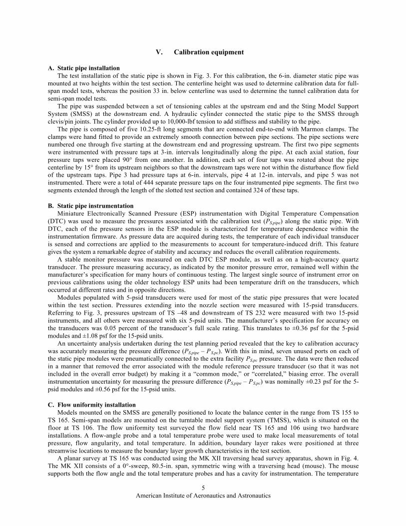
A. Static pipe installationThe test installation of the static pipe is shown in Fig. 3. For this calibration, the 6-in. diameter static pipe was

mounted at two heights within the test section. The centerline height was used to determine calibration data for full-span model tests, whereas the position 33 in. below centerline was used to determine the tunnel calibration data forsemi-span model tests.

The pipe was suspended between a set of tensioning cables at the upstream end and the Sting Model SupportSystem (SMSS) at the downstream end. A hydraulic cylinder connected the static pipe to the SMSS throughclevis/pin joints. The cylinder provided up to 10,000-lbf tension to add stiffness and stability to the pipe.

The pipe is composed of five 10.25-ft long segments that are connected end-to-end with Marmon clamps. Theclamps were hand fitted to provide an extremely smooth connection between pipe sections. The pipe sections werenumbered one through five starting at the downstream end and progressing upstream. The first two pipe segmentswere instrumented with pressure taps at 3-in. intervals longitudinally along the pipe. At each axial station, fourpressure taps were placed 90° from one another. In addition, each set of four taps was rotated about the pipecenterline by 15° from its upstream neighbors so that the downstream taps were not within the disturbance flow fieldof the upstream taps. Pipe 3 had pressure taps at 6-in. intervals, pipe 4 at 12-in. intervals, and pipe 5 was notinstrumented. There were a total of 444 separate pressure taps on the four instrumented pipe segments. The first twosegments extended through the length of the slotted test section and contained 324 of these taps.

B. Static pipe instrumentationMiniature Electronically Scanned Pressure (ESP) instrumentation with Digital Temperature Compensation

(DTC) was used to measure the pressures associated with the calibration test (PS,pipe) along the static pipe. WithDTC, each of the pressure sensors in the ESP module is characterized for temperature dependence within theinstrumentation firmware. As pressure data are acquired during tests, the temperature of each individual transduceris sensed and corrections are applied to the measurements to account for temperature-induced drift. This featuregives the system a remarkable degree of stability and accuracy and reduces the overall calibration requirements.

A stable monitor pressure was measured on each DTC ESP module, as well as on a high-accuracy quartztransducer. The pressure measuring accuracy, as indicated by the monitor pressure error, remained well within themanufacturer’s specification for many hours of continuous testing. The largest single source of instrument error onprevious calibrations using the older technology ESP units had been temperature drift on the transducers, whichoccurred at different rates and in opposite directions.

Modules populated with 5-psid transducers were used for most of the static pipe pressures that were locatedwithin the test section. Pressures extending into the nozzle section were measured with 15-psid transducers.Referring to Fig. 3, pressures upstream of TS –48 and downstream of TS 232 were measured with two 15-psidinstruments, and all others were measured with six 5-psid units. The manufacturer’s specification for accuracy onthe transducers was 0.05 percent of the transducer’s full scale rating. This translates to ±0.36 psf for the 5-psidmodules and ±1.08 psf for the 15-psid units.

An uncertainty analysis undertaken during the test planning period revealed that the key to calibration accuracywas accurately measuring the pressure difference (PS,pipe – PS,pc). With this in mind, seven unused ports on each ofthe static pipe modules were pneumatically connected to the extra facility PS,pc pressure. The data were then reducedin a manner that removed the error associated with the module reference pressure transducer (so that it was notincluded in the overall error budget) by making it a “common mode,” or “correlated,” biasing error. The overallinstrumentation uncertainty for measuring the pressure difference (PS,pipe – PS,pc) was nominally ±0.23 psf for the 5-psid modules and ±0.56 psf for the 15-psid units.

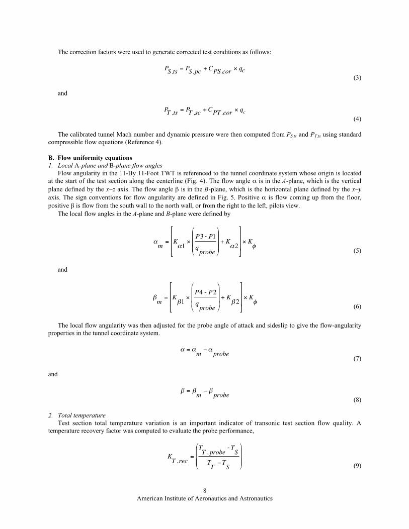
C. Flow uniformity installationModels mounted on the SMSS are generally positioned to locate the balance center in the range from TS 155 to

TS 165. Semi-span models are mounted on the turntable model support system (TMSS), which is situated on thefloor at TS 106. The flow uniformity test surveyed the flow field near TS 165 and 106 using two hardwareinstallations. A flow-angle probe and a total temperature probe were used to make local measurements of totalpressure, flow angularity, and total temperature. In addition, boundary layer rakes were positioned at threestreamwise locations to measure the boundary layer growth characteristics in the test section.

A planar survey at TS 165 was conducted using the MK XII traversing head survey apparatus, shown in Fig. 4.The MK XII consists of a 0°-sweep, 80.5-in. span, symmetric wing with a traversing head (mouse). The mousesupports both the flow angle and the total temperature probes and has a cavity for instrumentation. The temperature


probe was mounted 2.5-in. above the flow-angle probe. The mouse, which was remotely controlled, was traversedlaterally across the wing over a y = ±30 in. range. The entire apparatus was supported by sting hardware mounted tothe SMSS, allowing vertical translation of z = ±36 in. Stress load limitations prevented the MK XII from being usedat supersonic conditions, so it was replaced with a probe holder. This fixed the flow-angle probe position on thetunnel centerline (y = 0 in.) and the temperature probe at y = 3.5 in.

The same probe holder was used for a centerline survey at TS 106 over a vertical range of z = –54 to24 in. For this measurement, the floor slot baffles were removed and replaced with solid fillers to provide thereflection plane necessary for semi-span model testing.

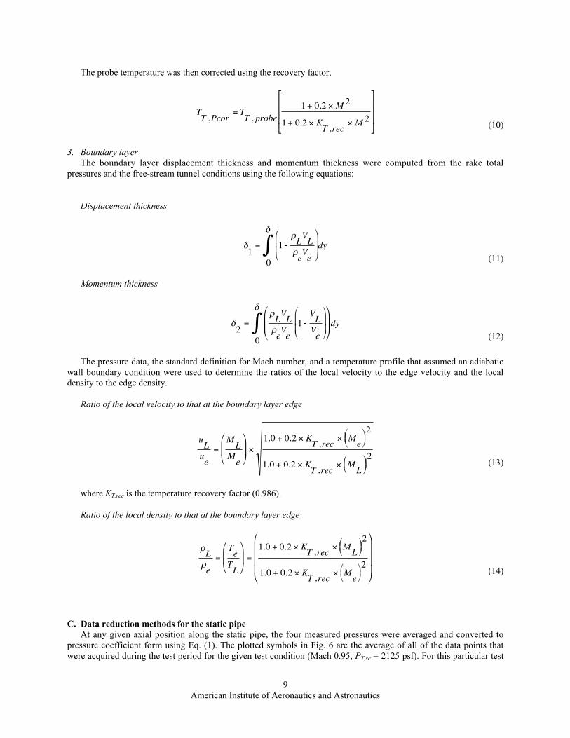
D. Flow uniformity instrumentationFlow-angularity and total pressure data were collected from a five-hole cone probe with holes arranged on a 40°

conical nose and a set of static-sensing taps arranged on the aft body (Fig. 5). Pressure differences across the conewere measured using temperature-compensated, 1-psid pressure transducers. The manufacturer-quoted accuraciesare 0.06 percent “best straight line” with ±0.025 percent of full scale per °F for thermal zero shift and ±0.01 percentof reading per °F for thermal sensitivity shift. The transducers were calibrated at the NASA Ames Metrology labusing equipment traceable to NIST standards. The probe total and static pressures were each plumbed to eight portson a 15-psid, DTC ESP module.

Probe angle of attack was measured using a precision accelerometer. The accelerometer was placed in thetraversing head for the MK XII installation and in the instrumentation cavity on the supersonic probe holder.Accelerometers were calibrated at the NASA Ames Metrology lab and re-zeroed in the test section against astandard with an accuracy of 0.005°. Probe sideslip angle was measured using the SMSS knuckle-sleeve device,which uses a pair of rotating bent arms called the knuckle and the sleeve to obtain taper angles in the pitch and yawplanes anywhere between ±15°. The angular offsets between the probe tip and the angle measurement devices werecarefully measured and accounted for in the data reduction. The horizontal position of the probe along the y-axis wasmeasured using an encoder, and the vertical position along the z-axis were measured using a string pot.

Test section total temperature TT,probe was measured with an RTD mounted in a shielded probe holder. Theaccuracy of this airflow probe was stated by the manufacturer to be ±2.0 °F.

Boundary layer characteristics were defined from measurements using three 10-in.-high rakes. Each rake wasinstrumented with twenty 0.04-in.-diameter pitot probes. The probes were plumbed to 15-psid transducers on DTCESP modules. The boundary layer rakes were positioned on the test section floor with rake 1 at x = 36 in., y = 0 in.;rake 2 at x = 106 in., y = 10.4 in.; and rake 3 at x = 176 in., y = –10.4 in.

Redundant facility PT,sc and PS,pc pressures were measured using eight ports on the same DTC ESP modules usedfor the flow-angle probe pressures. As with the static pipe, these pressures were used in the data reduction tominimize the bias error associated with the ESP module reference pressure.

VI. Data acquisitionSteady-state data were acquired using the wind tunnel facility’s Standard Data System (SDS). The SDS consists

of a Subsystem Management Processor (SMP), a number of Functional Subsystem Processors (FSPs), and a largenumber of X-terminals that provide wind tunnel personnel with graphical user interfaces to the features of SDS. TheSMP is an Enterprise 3500 server (Sun Microsystems, Santa Clara, CA) running the Solaris operating system. TheSMP manages the overall data acquisition activity in a facility. Its tasks include coordinating the FSPs, interfacingwith the automated tunnel condition and model attitude control systems, and providing a command and controlinterface for operations personnel. The SMP also provides visualization and analysis tools for both the real-time andnear-time data streams. FSPs are Pentium-class PCs running LynxOS Real-Time UNIX (Lynx Real-Time Systems,Inc.). These modular units are responsible for collecting data from particular types of sensors. The six FSPinstrument categories are balance, surface pressure, digital, general purpose analog, tunnel condition/model attitude,and temperature. Each FSP was designed to perform instrument-specific data acquisition tasks for collecting thehighest quality data at the sensor and instrument’s maximum throughput. Sensor data are transmitted in parallelacross a 100 Base-T Ethernet highway to the SMP, where they are averaged, converted to common engineeringunits, and further reduced to test-specific final results.

A. Static pipe data acquisition


The static pipe test provided one set of calibration tables for sting-mounted models and a second set forturntable-mounted semi-span models. The calibration tables for semi-span testing were measured with the static pipelocated 33 in. below the tunnel centerline, which more closely matches the model reference point of semi-spanmodels. Data were normally recorded in groups of six data points with a 30-sec delay programmed between datapoints. Several of the calibration test conditions were repeated up to five times over the duration of the test so thatrepeatability statistics could be extracted from the test database. All data were acquired using a one second samplingperiod, which was determined to be optimum during an initial sampling study. The reference pressure used for thestatic pipe ESP modules was a steady “driven” or controlled pressure and was set to be within ±0.5 psi of the tunnelstatic pressure as the tunnel was set to the desired Mach number and total pressure. Pressures were allowed to settlefor several minutes before data were taken at the new tunnel conditions.

B. Flow uniformity data acquisitionTest section flow properties were measured at Mach numbers of 0.4, 0.6, 0.8, 0.85, 1.2, and 1.4 and at total

pressures of 2120, 3180, and 4600 psf. A sampling study was initially performed, and a one second duration waschosen for data acquisition. A flow-angle probe calibration was performed at 3180 psf for subsonic Mach numbersand at 2120 psf for supersonic Mach numbers with the flow-angle probe on the centerline at TS 165. The calibrationinvolved pitching the probe from –2° to 2° in 0.25° increments for four probe orientations, φ = 0°, 180°, 90°, and270°. The MK XII survey apparatus was then installed, and the planar survey was conducted at TS 165. The mousewas traversed horizontally from y = –30 to 30 in., in 6-in. increments. At each horizontal position, the surveyapparatus was traversed from z = –36 to 36 in., in 6-in. increments. After the survey was completed for a giventunnel conditions set point, the next calibration condition was set and the probe positioning was conducted in thereverse order. For the supersonic test conditions, the MK XII was replaced with the probe holder and a centerlinesurvey was conducted from z = –36 to 36 in., in 6-in. increments.

For evaluating the flow uniformity for the semi-span model test, the centerline survey hardware was moved toTS 106 and the slot baffles were removed from the test section floor and replaced with solid fillers. The centerlinesurvey was conducted from z = –54 to 24 in., in 6-in. increments. Boundary layer rakes were initially installed in thetest section for the survey at TS 165 but were removed when they interfered with the flow-angle measurements atthe supersonic conditions.

VII. Data reduction

A. Calibration equationsThe static pipe and flow uniformity tests provide the calibration tables to correct the facility's institutional total

and static pressure measurement to the true total and static pressure in the test section. The tables provide onecorrection factor for static pressure, CPS,cor, and a second factor for total pressure, CPT,cor. These factors are defined asfollows:

€

CPS,cor =PS,pipe − PS,pc

qc

(1)

and

€

CPT ,cor =PT ,probe − PT ,sc

qC

(2)

Each of the calibration tables contains entries for 38 test section locations at 3-in. intervals, 15 Mach numbers,and 4 total pressures. When a data reduction program is set up for a test project, the streamwise location of themodel reference point in the test section and the test type (full-span or semi-span) are specified. A lookup table isthen extracted from the calibration table, which includes correction factors at the 15 calibrated Mach numbers and 4calibrated total pressures. During the test project, this table was used to obtain correction factors for PT,sc and PS,pc.For intermediate points between the calibrated test conditions, linear interpolation was performed on both PT,sc andMc to arrive at the proper correction factors. Linear extrapolation was used to determine the correction factors forpoints outside the calibrated test conditions.


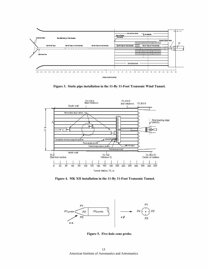
The correction factors were used to generate corrected test conditions as follows:

€

PS,ts = PS,pc + CPS,cor × qc(3)

and

€

PT ,ts = PT ,sc + CPT ,cor × qc(4)

The calibrated tunnel Mach number and dynamic pressure were then computed from PS,ts and PT,ts using standardcompressible flow equations (Reference 4).

B. Flow uniformity equations1. Local A-plane and B-plane flow angles

Flow angularity in the 11-By 11-Foot TWT is referenced to the tunnel coordinate system whose origin is locatedat the start of the test section along the centerline (Fig. 4). The flow angle α is in the A-plane, which is the verticalplane defined by the x–z axis. The flow angle β is in the B-plane, which is the horizontal plane defined by the x–yaxis. The sign conventions for flow angularity are defined in Fig. 5. Positive α is flow coming up from the floor,positive β is flow from the south wall to the north wall, or from the right to the left, pilots view.

The local flow angles in the A-plane and B-plane were defined by

€

αm = Kα1 ×

P3 - P1qprobe

+ Kα2

× K

φ(5)

and

€

βm = Kβ1 ×

P4 - P2qprobe

+ Kβ 2

× K

φ(6)

The local flow angularity was then adjusted for the probe angle of attack and sideslip to give the flow-angularityproperties in the tunnel coordinate system.

€

α = αm −α probe(7)

and

€

β = βm − β probe(8)

2. Total temperatureTest section total temperature variation is an important indicator of transonic test section flow quality. A

temperature recovery factor was computed to evaluate the probe performance,

€

KT ,rec =TT , probe - TS

TT −TS

(9)


The probe temperature was then corrected using the recovery factor,

€

TT ,Pcor = TT , probe1+ 0.2 × M 2

1+ 0.2 × KT ,rec × M2

(10)

3. Boundary layerThe boundary layer displacement thickness and momentum thickness were computed from the rake total

pressures and the free-stream tunnel conditions using the following equations:

Displacement thickness

€

δ1 = 1 -ρLVLρeVe

0

δ

∫ dy(11)

Momentum thickness

€

δ2 =ρLVLρeVe

1 -VLVe

dy

0

δ

∫(12)

The pressure data, the standard definition for Mach number, and a temperature profile that assumed an adiabaticwall boundary condition were used to determine the ratios of the local velocity to the edge velocity and the localdensity to the edge density.

Ratio of the local velocity to that at the boundary layer edge

€

uLue

=MLMe

×

1.0 + 0.2 × KT ,rec × Me

2

1.0 + 0.2 × KT ,rec × ML

2

(13)

where KT,rec is the temperature recovery factor (0.986).

Ratio of the local density to that at the boundary layer edge

€

ρLρe

=TeTL

=

1.0 + 0.2 × KT ,rec × ML

2

1.0 + 0.2 × KT ,rec × Me

2

(14)

C. Data reduction methods for the static pipeAt any given axial position along the static pipe, the four measured pressures were averaged and converted to

pressure coefficient form using Eq. (1). The plotted symbols in Fig. 6 are the average of all of the data points thatwere acquired during the test period for the given test condition (Mach 0.95, PT,sc = 2125 psf). For this particular test


condition, each symbol is an average of 120 data points. The heavy solid line in Fig. 6 is a plot of a smoothing curvefit determined from the set of averaged data. A polynomial curve fit method was used for all calibration data fromMach 0.2 through 1.0. For supersonic test conditions, a “boxcar” smoothing algorithm was used because thepressure distributions did not fit the polynomial pattern. Weak tunnel- and static-pipe-generated shocks andexpansions caused the more erratic pressure distributions that were measured at supersonic conditions. Curve fitresults were used to generate both the tunnel control system tables for setting tunnel Mach number and Reynoldsnumber and data-reduction system tables for computing Mach numbers and Reynolds numbers for test projects.

D. Data reduction methods for flow uniformityEstablished procedures were used for calibrating the five-hole cone probe in the test section for various Mach

numbers at a tunnel total pressure of 3180 psf. These procedures involved pitching the probe at four rollorientations, φ = 0°, 180°, 90°, and 270°. Calibration constants derived from calibration runs were applied to themeasured pressure data to compute the local flow-angularity properties of the tunnel using Eq. (5) to (8). Data werethen processed using commercially available data analysis software to produce flow-angle vector plots. An averagerecovery factor of 0.94 was determined from the temperature data and used to compute the corrected temperature inthe test section for all runs.

VIII. Calibration results

A. Factors affecting the static pipe calibration results

1. Temporal variation of test section flowThe standard deviations of the pipe Cp’s at Mach 0.95 and PT,sc = 2125 psf are presented in Fig. 7. The data

points were recorded once per second for 120 sec. The odd shape shown in Fig. 7 with its minimum point near TS230 and continuously varying standard deviation is caused by a combination of pneumatic lag in the pressure tubingof the pipe and a low-frequency, small-amplitude time variation of test section static pressure. The pressure-scanning modules were mounted in the instrumentation enclosure of the SMSS. The pressure tubing from themodule to the port, therefore, increased in length from the ports at the downstream end of the pipe to the upstreamend.

A comparison of the time variation of the facility reference static pressure PS,pc and the measured static pipepressure at TS 230 (the standard deviation minimum point in Fig. 7) is presented in Fig. 8. The normalizeddeviations of the two pressures are compared so that time correlation is clearly illustrated within a single figure.Both the phasing and standard deviation of the time variation of these two pressures are nearly identical. Thecorrelation coefficient of the two pressures is indicated on the figure as 0.997. At this location on the static pipe, thepneumatic damping characteristic of the tubing is equal to the damping of the PS,pc pressure tubing. At TS 110, thepressure tubing connecting the static pipe port to the pressure scanning module is 120 in. longer than it is for the tapsat TS 230. The comparison of the normalized deviation of the pipe pressure at this location is shown in Fig. 9. Thisfigure shows that the pipe pressure at TS 110 is lagging in time and has a reduced standard deviation with respect tothe PS,pc pressure. At TS 0, the pressure tubing connecting the static pipe port to the pressure scanning module is 230inches longer than it is for the taps at TS 230. Figure 10 shows that this pipe pressure lags more and shows a furtherreduced standard deviation with respect to PS,pc. The effect of the combination of the tunnel time varying flow andthe pneumatic tubing damping/lag differences results in added precision uncertainty averaging about ±0.001 to themeasured static pipe pressure coefficients. Smoothing by curve fit and averaging of multiple data points negatesmost of the effects of this source of data inaccuracy.

2. Effects of test section slotsCurve fits for the semi-span calibration for Mach 0.6 to 1.0 are shown in Fig. 11. The negative pressure gradient

at the start of the test section is attributed to the relieving effects of the test section slots, which start at TS 0.

3. Mounting interference effectsReferring again to Fig. 11, the positive pressure gradient near the downstream end of the test section is believed

to be caused by interference effects from the static pipe hydraulic cylinder fairing and the 11-By 11-Foot TWTSMSS, which feed forward into the test section. Since the shape and volume of the static pipe fairing is similar to thestings and adapters commonly used to support sting-mounted models, no additional Mach corrections are currently


used to account for this mounting interference. This pressure distribution is used to compute a clear tunnel buoyancycorrection that is applied to the measured model forces.

4. Tap error and pipe joint effectsThe curve fit residuals (Cpm – Cpfit) for the Mach range from 0.6 to 1.0 are shown in Fig. 12. The residuals are

caused by tap error in the pipe pressure measurements. Tap error is a result oflocal imperfections at the tap or on the pipe surface in the neighborhood of the tap. It can be seen in Fig. 12 that thecurve fit residuals are nearly identical for this range of test section Mach number, which infers that the residuals arean artifact of the pipe or pipe taps rather than of the flow in the tunnel. The static pipe is also used to calibrate the12-Foot Pressure Wind Tunnel. Results from the 12-Foot Pressure Wind Tunnel facility calibration were comparedwith those seen in Fig. 12 and showed remarkably similar residuals. This suggests that tap error is the cause of thesmall-scale variation in measured pressure along the test section length and that it justifies the smoothing procedureused in the calibration data reduction. The large residuals shown near TS 5 and 125 coincide with the joints in thestatic pipe assembly between adjacent 10.25-ft pipe sections (see Fig. 3).

5. Instrumentation error effectsDuring the planning phases of the static pipe calibration, uncertainty analysis was used to guide choices of

instrumentation, instrumentation hookup, and data-reduction procedures. Figure 13 shows the results of theseuncertainty analyses for the actual instrumentation, instrument hookup, and data reduction program that was used.The goal for the calibration was to limit the Mach errors due to the instrument error sources to ±0.001 for all testconditions within the test matrix. On the basis of the data checking and repeat data points that were recorded duringthe calibration, the instrumentation performed to the specifications claimed by the manufacturers.

B. Calibration results for the static pipe

1. Mach number effectsThe effect of Mach variation on the test section Cp for subsonic and supersonic operation can be seen in Fig. 14

and Fig. 15, respectively. Within these figures, the Mach number is varied while the facility total pressure ismaintained at 2125 psf. The most noticeable trends shown in Fig. 14 are the increase in the slot effect for increasingMach number at TS 0 and the decrease in the “forward feeding” interference effect of the static pipe fairing and thesting model support for increasing Mach numbers. For supersonic Mach numbers (Fig. 15), the obvious change is agreater longitudinal variation of the Cp in comparison to subsonic values, especially in the forward half of the testsection. These effects are attributable to the discontinuity in the wall boundary condition where the test section slotsbegin. Small mass additions through the slots produce diffuse tunnel shocks that originate in the first foot of the testsection. A second obvious difference between the subsonic and supersonic Cp distributions is the absence of apressure influence from the pipe hydraulic cylinder fairing and the SMSS at the downstream end of the static pipe.The supersonic test section flow effectively eliminates upstream propagation of the pressure disturbance arisingfrom the fairing and support system.

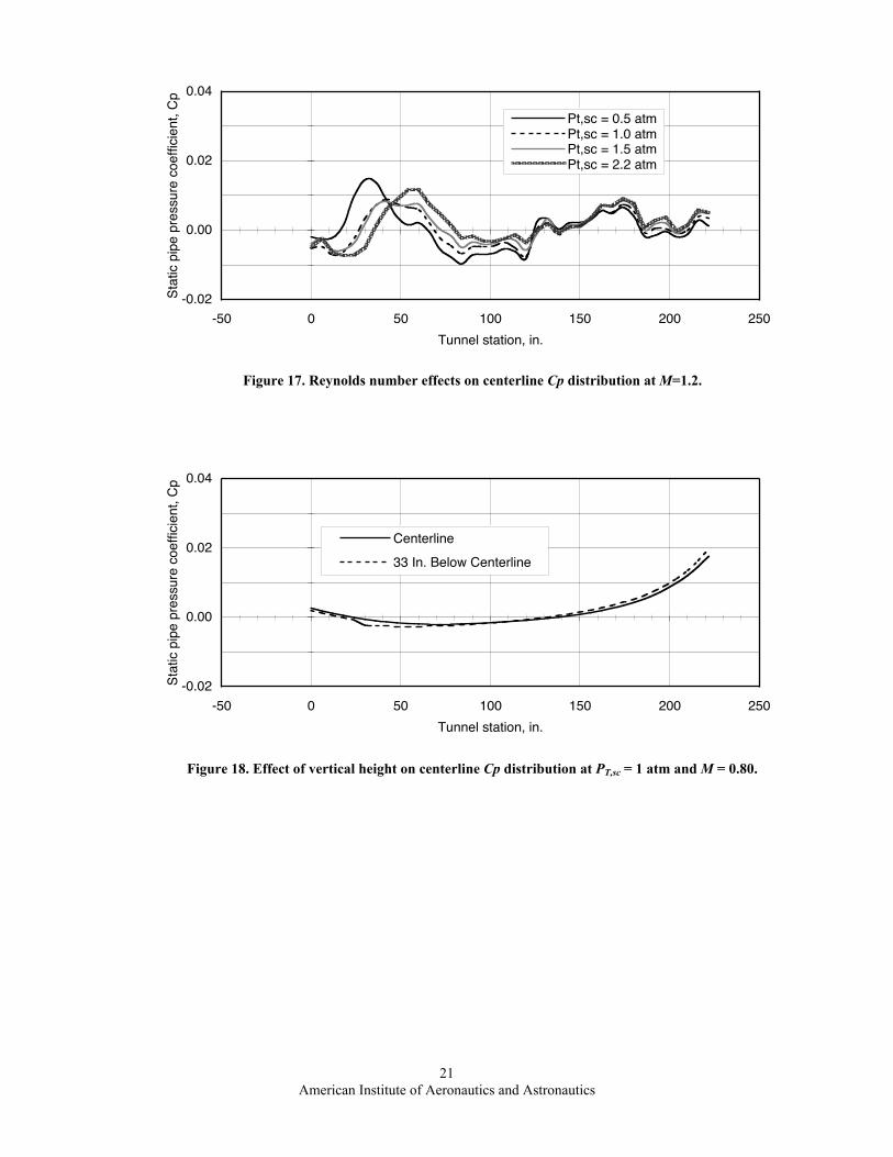
2. Reynolds number effectsSubsonic and supersonic Reynolds number effects on the test section Cp distribution are summarized in Fig. 16

and Fig. 17, respectively. The Mach number is fixed for the data contained within the figures, whereas the tunneltotal pressure is varied through the setpoint values of 0.5, 1.0, 1.5, and 2.2 atm. In Fig. 16, a Mach number of 0.8was chosen to illustrate the Reynolds number effects at subsonic test conditions. The effects shown are small butsystematic. There appears to be a Cp increase that varies with tunnel total pressure. The most likely cause for thisphenomenon is the change in test section boundary layer growth that occurs at the different Reynolds numbers.Boundary layer growth forces differing amounts of slot cross flow and consequent changes in the pressuredifferential between the plenum chamber and test section. Figure 17 illustrates the Reynolds number effects forMach 1.2. The most obvious difference between the supersonic and subsonic Reynolds number effects is thepressure disturbance that appears on the static pipe 20 to 70 in. downstream of the start of the test section slots. Thedisturbance is believed to be caused by diffuse tunnel shocks that arise near the slot origin in response to the slightchanges in slot mass flow.


3. Centerline versus 33 in. below centerlineFigure 18 shows the difference between the Cp distribution on the tunnel centerline and 33 in. below the

centerline for Mach 0.8. These differences are minor in the regions where most wind tunnel models are positioned:TS 106 for semi-span models and TS 155 to 165 for full-span models.

C. Calibration results for flow uniformity

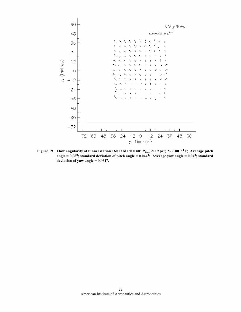
1. Flow angleFlow-angularity results for Mach 0.8 and PT,sc = 3180 psf at TS 165 are presented in Fig. 19. For the planar

survey, measurements were made over the range defined by y = ±36 in. and z = ±36 in. The vector plot shows verysmall flow angles especially in the core region where models are tested. Statistics for all the measurements in thisplane yield an average and standard deviation of 0.08° and 0.044° for the A-plane flow angle and 0.04° and 0.061°for the B-plane flow angle. The slightly larger flow angles measured closest to the tunnel walls may be a result ofthe flow field being deflected by the survey apparatus itself. Premodernization flow-angle surveys measured largeflow-angle gradients on the centerline within several feet of the test section floor. Values for α and β were as muchas 0.35° at z = –26.4 in. Figure 19 clearly shows that this anomaly is no longer present in the flow. The improvementin the test section flow angularity is attributed to the addition of the honeycomb in the settling chamber.

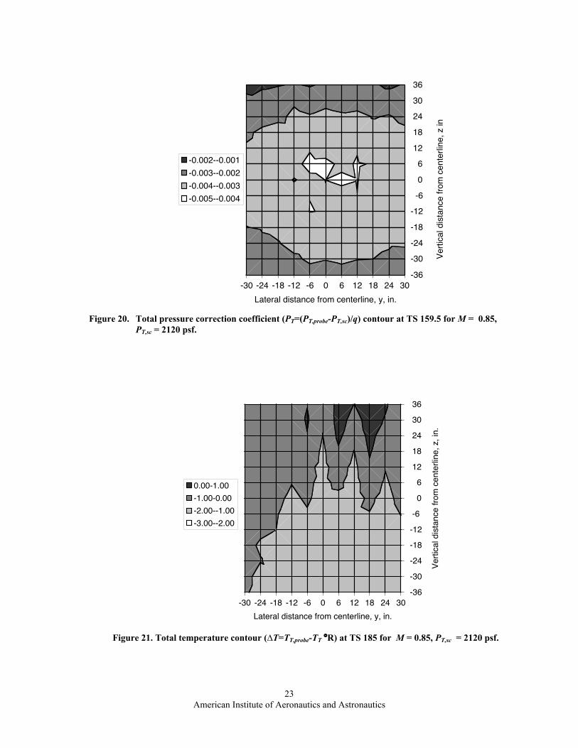
2. Total pressureThe total pressure variation for Mach 0.85 and PT,sc = 2120 psf is presented using a contour plot of CPT,cor (Fig.

20). The figure shows a small variation in the test section total pressure from that measured by the facility probes.Values for CPT,cor are largest at the centerline and drop to zero near the test section walls. Measurements made in thetest section prior to the addition of the TRS showed good agreement with those measured by the facility totalpressure probes. At that time, facility total pressure was measured using probes located on the centerline, mountedoff the turning vane set just upstream of the contraction. The variation in PT shown in Fig. 20 is a result of theintroduction of the TRS. Pressure losses resulting from the honeycomb and screens are a function of the dynamicpressure entering the TRS, which varies across the radius. Pressure loss across the TRS is, therefore, nonuniformand largest at the centerline.

3. Total temperatureThe total temperature variation for Mach 0.85 and PT,sc = 2120 psf is presented in Fig. 21 using a contour plot of

ΔT = (TT,probe – TT,F). The data show a slight increase in the total temperature above the centerline, but the levelsmeasured are within 2 °F.

4. Boundary layerBoundary layer measurements are useful for determining the proper standoff height for semi-span models.

Figures 22 and 23 present the displacement thickness and momentum thickness for Mach 0.4 and 0.8 for PT,sc =3180 psf from three sets of data. Data at TS 36 are for floor slots normal, which is influenced by flow exchangebetween the test section and the plenum. Data at TS 176 are with the floor sealed and give the upper bound fordetermining the proper standoff height for semi-span models. Data at TS 106 are from a premodernization test withthe floor slots sealed and are within the bound defined by the data at TS 176.

IX. ConclusionA series of calibration and flow survey tests were conducted in the 11-by 11-Foot TWT. The objective of these

tests was to determine the test section static and total pressure calibration tables for the full-span and semi-span testsection configurations. A static pipe was used to measure the longitudinal static pressure distribution through thenozzle and test section. A survey rake was used to measure the total pressure, total temperature and flow angleuniformity at two tunnel stations.

Results from the static pipe test identified several factors that influenced the measurements. These includedeffects of the slots, the effect of the mounting hardware, tap and pipe joint effects and the selection ofinstrumentation. In addition, variations in the static pressure with both Mach number and Reynolds and minordifferences with the pipe at centerline and 33 inches below centerline were observed. The calibration tables weredetermined from curve-fits of the data. The flow uniformity survey showed improvements in the flow angularityand identified a small loss in total pressure due to the addition of the TRS.


A key to the success of the calibration was the use of uncertainty analysis early on to select the instrumentationthereby limiting the error in Mach number measurement to within the goal of 0.001.

References

1 Kmak, F.J., “Modernization and Activation of the NASA Ames 11-By 11-Foot Transonic Wind Tunnel”, Paper# 2000-2680, 21st AIAA Advanced Measurement and Ground Testing Technology Conference, Denver, CO, June 19-20, 2000.

2 Kmak, F., Hudgins, M., and Hergert, D., “Revalidation of the NASA Ames 11-By 11-Foot Transonic Wind Tunnel With aCommercial Airplane Model”, Paper# 2001-0454, 39th AIAA Aerospace Sciences Meeting & Exhibit, Reno, NV, January 8-11,2001.

3 Amaya, M.A., and Murthy, S.V., “Flow Quality Measurements in the NASA Ames Upgraded 11-By 11-Ft Transonic WindTunnel”, Paper# 2000-2681, 21st AIAA Advanced Measurement and Ground Testing Technology Conference, Denver, CO, June19-20, 2000.

4 NASA Ames Research Staff, “Equations, Tables and Charts for Compressible Flow”, NACA TR-1135, 1953.


Appendix

Figure 1. Unitary Plan Wind Tunnel (UPWT) At the NASA Ames Research Center.

Figure 2. 11-By 11-Foot Transonic Wind Tunnel.


300280260240220200160 180

4.75"

-40 -20 0 20 40 60 80 100 120 140

Start of SlottedTest Section

T.S.165

-60-80-100-120-140-180 -160--380 -360 -340 -320 -300 -280 -260 -240 -220 -200

C.R.

Pipe #1 (Taps at 3 Inch Intervals)Pipe #2 (Taps at 3 Inch Intervals)Pipe #3 (Taps at 6 Inch Intervals)Pipe #4 (Taps at 12 Inch Intervals)Pipe #5 (No Taps )

Hydraulic Cylinder FairingFlex Wall Entry to Test SectionTensioning Cables

Ogive Nose Cone

TUNNEL STATION IN INCHES

Figure 1. - Static Pipe Installation in the ARC 11 Foot TWT

TEST SECTION FLOOR

TEST SECTION CEILING C OF WINDOWS

Figure 3. Static pipe installation in the 11-By 11-Foot Transonic Wind Tunnel.

Figure 4. MK XII installation in the 11-By 11-Foot Transonic Tunnel.

Figure 5. Five-hole cone probe.


-0.05

0.00

0.05

0.10

0.15

-50 0 50 100 150 200 250Tunnel station, in.

Pres

sure

Coe

fficie

nt(P

s,ts

-Ps,

pc)/q

c

Mc=0.95Curve fit

Figure 6. Average centerline Cp distribution and curve fit for M = 0.95, PT,sc = 2125 psf; Sample durationis 1.0 second; number of data points, 120.

0.000

0.001

0.002

0.003


Stan

dard

Dev

iatio

n in

Cp

Mc=0.95

Figure 7. Standard deviation in the centerline Cp distribution for M = 0.95, PT,sc = 2125 psf; Sampleduration is 1.0 second; number of data points, 120.


-5.0

-4.0

-3.0

-2.0

-1.0

0.0

1.0

2.0

3.0

4.0

5.0

0 10 20 30 40 50 60 70 80 90 100 110 120Time, sec

Ps,p

c an

d Ps

,ts=1

10 v

aria

tion,

(P-P

avg)

/σ

Ps at TS 110Ps,pc,var

Correlation Coefficient = 0.799

Figure 9. Temporal variation of test section pressure at tunnel station 110 for for M = 0.95, PT,sc = 2125 psf;Sample duration, 1 sec; correlation coefficient, 0.799; PS,pc, 1187.7 psf; σPS,pc, 1.29 psf;PS,pipe,avg, 1185.60 psf; σPS,pipe, 0.84 psf.

-5.0

-4.0

-3.0

-2.0

-1.0

0.0

1.0

2.0

3.0

4.0

5.0

0 10 20 30 40 50 60 70 80 90 100 110 120Time, sec

Ps,p

c an

d Ps

,ts=2

30 v

aria

tion,

(P-P

avg)

/σ

Ps at TS 230Ps,pc,var


Figure 8. Temporal variation of test section pressure at tunnel station 230 for M = 0.95, PT,sc = 2125 psf;Sample duration, 1 sec; correlation coefficient, 0.9970; PS,pc, 1187.7 psf; σPs,pc, 1.29 psf;PS,pipe,avg, 1204.97 psf; σPS,pipe, 1.22 psf.


-5.0

-4.0

-3.0

-2.0

-1.0

0.0

1.0

2.0

3.0

4.0

5.0

0 10 20 30 40 50 60 70 80 90 100 110 120Time, sec

Ps,p

c an

d Ps

,ts=0

var

iatio

n, (P

-Pav

g)/σ

Ps at TS 0Ps,pc,var


Figure 10. Temporal variation of test section pressure at tunnel station 0 for for M = 0.95, PT,sc = 2125 psf;Sample duration, 1 sec; correlation coefficient, 0.656; PS,pc, 1187.7 psf; sPs,pc, 1.29 psf;PS,pipe,avg, 1193.25 psf; sPS,pipe, 0.72 psf.

-0.02

-0.01

0.00

0.01

0.02

0.03

0.04

0.05

0.06


Stat

ic pr

essu

re c

oeffi

cient

, Cp

M = 0.6M = 0.8M = 0.9M = 1.0

Figure 11. Effect of test section slots on centerline static pipe Cp distribution, PT,sc = 2127 psf.


-0.008

-0.006

-0.004

-0.002

0.000

0.002

0.004

0.006

0.008


Cp d

ata

fit re

sidua

ls

M = 0.6M = 0.8M = 0.9M = 1.0

Figure 12. Tap error distribution along static pipe, PT,sc = 2127 psf.

0.0000

0.0004

0.0008

0.0012

0.0016

0.0020

0.0 0.2 0.4 0.6 0.8 1.0 1.2 1.4 1.6Test Section Mach Number

Pipe

Mac

h Nu

mbe

r Unc

erta

inty

Pt,sc = 0.5 atmPt,sc = 1.0 atmPt,sc = 1.5 atmPt,sc = 2.2 atm

Uncertainty Goal

Figure 13. Uncertainty analysis predictions based on ±5 psid DTC pressure scanning modules and flowreference system.


-0.02

0.00

0.02

0.04


Stat

ic pi

pe p

ress

ure

coef

ficie

nt, C

p

M = 0.6 M = 0.8M = 0.9M = 1.0

Figure 14. Subsonic Mach number effects on centerline Cp distribution at PT,sc = 2125 psf.

-0.02

0.00

0.02

0.04


Stat

ic pi

pe p

ress

ure

coef

ficie

nt, C

p

M = 1.1M = 1.2M = 1.3M = 1.4

Figure 15. Supersonic Mach number effects on centerline Cp distribution at PT,sc = 2125 psf.

-0.02

0.00

0.02

0.04


Stat

ic pi

pe p

ress

ure

coef

ficie

nt, C

p


Figure 16. Reynolds number effects on centerline Cp distribution at M=0.8.


-0.02

0.00

0.02

0.04


Stat

ic pi

pe p

ress

ure

coef

ficie

nt, C

p

Centerline33 In. Below Centerline

Figure 18. Effect of vertical height on centerline Cp distribution at PT,sc = 1 atm and M = 0.80.

-0.02

0.00

0.02

0.04


Stat

ic pi

pe p

ress

ure

coef

ficie

nt, C

p


Figure 17. Reynolds number effects on centerline Cp distribution at M=1.2.


Figure 19. Flow angularity at tunnel station 160 at Mach 0.80; PT,sc, 2119 psf; TT,F, 80.7 °F; Average pitchangle = 0.08°; standard deviation of pitch angle = 0.044°; Average yaw angle = 0.04°; standarddeviation of yaw angle = 0.061°.


-36

-30 -24

-18

-12 -6

0

6 12

18

24 30

36

-30 -24 -18 -12 -6 0 6 12 18 24 30Lateral distance from centerline, y, in.

Verti

cal d

istan

ce fr

om c

ente

rline

, z in

-0.002--0.001-0.003--0.002-0.004--0.003-0.005--0.004

Figure 20. Total pressure correction coefficient (PT=(PT,probe-PT,sc)/q) contour at TS 159.5 for M = 0.85,PT,sc = 2120 psf.

-30 -24 -18 -12 -6 0 6 12 18 24 30 -36

-30

-24

-18

-12

-6

0

6

12

18

24

30

36

Lateral distance from centerline, y, in.

Verti

cal d

istan

ce fr

om c

ente

rline

, z, i

n.

0.00-1.00-1.00-0.00-2.00--1.00-3.00--2.00

Figure 21. Total temperature contour (∆T=TT,probe-TT °R) at TS 185 for M = 0.85, PT,sc = 2120 psf.


0

0.2

0.4

0.6

0.8

1

0 50 100 150 200Tunnel station, in.

Disp

lace

men

t thi

ckne

ss, δ1 ,

in. Mc = 0.4, Slots Normal Mc = 0.8, Slots Normal

Mc = 0.4, Solid Floor Mc = 0.8, Solid FloorMc = 0.4, Solid Floor Mc = 0.8, Solid Floor

Figure 22. Boundary layer displacement thickness at M=0.4 and M=0.8 for PT,sc = 3180 psf.

0

0.2

0.4

0.6

0.8

1

0 50 100 150 200Tunnel station, in.

Mom

entu

m th

ickne

ss, δ

2, in

. Mc = 0.4, Slots Normal Mc = 0.8, Slots NormalMc = 0.4, Solid Floor Mc = 0.8, Solid FloorMc = 0.4, Solid Floor Mc = 0.8, Solid Floor

Figure 23. Boundary layer momentum thickness at M=0.4 and M=0.8 for PT,sc = 3180 psf.

calibration of the 11-by 11-foot transonic wind … institute of aeronautics and astronautics 1...

Documents