c american institute of mathematical sciences 1 pp. 149{180

Mathematical Foundations of Computing doi:10.3934/mfc.2018008c©American Institute of Mathematical SciencesVolume 1, Number 2, May 2018 pp. 149–180

HOW CONVOLUTIONAL NEURAL NETWORKS SEE THE

WORLD — A SURVEY OF CONVOLUTIONAL NEURAL

NETWORK VISUALIZATION METHODS

Zhuwei Qin††George Mason University

4400 University Dr, Fairfax, VA 22030, USA

Fuxun Yu†, Chenchen Liu‡ and Xiang Chen†∗

‡Clarkson University

8 Clarkson Ave, Potsdam, NY 13699, USA

(Communicated by Zhipeng Cai)

Abstract. Nowadays, the Convolutional Neural Networks (CNNs) have

achieved impressive performance on many computer vision related tasks, suchas object detection, image recognition, image retrieval, etc. These achievements

benefit from the CNNs’ outstanding capability to learn the input features with

deep layers of neuron structures and iterative training process. However, theselearned features are hard to identify and interpret from a human vision perspec-

tive, causing a lack of understanding of the CNNs’ internal working mechanism.

To improve the CNN interpretability, the CNN visualization is well utilized as aqualitative analysis method, which translates the internal features into visually

perceptible patterns. And many CNN visualization works have been proposed

in the literature to interpret the CNN in perspectives of network structure,operation, and semantic concept.

In this paper, we expect to provide a comprehensive survey of several rep-

resentative CNN visualization methods, including Activation Maximization,Network Inversion, Deconvolutional Neural Networks (DeconvNet), and Net-

work Dissection based visualization. These methods are presented in terms ofmotivations, algorithms, and experiment results. Based on these visualization

methods, we also discuss their practical applications to demonstrate the sig-

nificance of the CNN interpretability in areas of network design, optimization,security enhancement, etc.

1. Introduction. The Convolutional Neural Networks (CNNs) have been widelyinvestigated as one of the most promising solutions for various computer visionrelated tasks, such as object detection [20, 58], image recognition [36, 63, 66, 27],image retrieval [22, 25], etc.

Inspired by the hierarchical organization of the human visual cortex [34], theCNN is constructed with many intricately interconnected layers of neuron struc-tures. These neurons act as the basic units to learn and extract certain featuresfrom the input. With the network complexity increment caused by the neuron layer

2010 Mathematics Subject Classification. Primary: 58F15, 58F17; Secondary: 53C35.Key words and phrases. Deep learning, convolutional neural network, CNN feature, CNN vi-

sualization, network interpretability.The authors are supported by NSF Grant CNS-1717775.∗ Corresponding Author: Xiang Chen.

1

arX

iv:1

804.

1119

1v2

[cs

.CV

] 3

1 M

ay 2

018

http://dx.doi.org/10.3934/mfc.2018008

2 ZHUWEI QIN, FUNXUN YU, CHENCHEN LIU AND XIANG CHEN

depth, the performance of the input feature extraction is also enhanced. For exam-ple, AlexNet – one of the most representative CNNs, has 650K neurons and 60Mrelated parameters [36]. Also, sophisticated algorithms are proposed to support thetraining and testing of such a complex network, and the backpropagation method iswidely applied to train the CNN parameters through multiple layers [39, 44]. Fur-thermore, to fine-tune the network to specific functions, large pools of labeled dataare required for iteratively training the massive neurons and connection weights. Sofar, many high-performance CNN designs have been proposed, such as AlexNet [36],VGG [63], GoogleNet [66], ResNet [27], etc. Some of the designs can even achievebeyond human-level accuracy on object recognition tasks [61].

Although the CNNs can achieve competitive classification accuracy, the CNNsstill suffer from high computational cost, slow training speed, and security vulner-ability [67, 38, 4]. One major reason causing these shortcomings is the lack of net-work interpretability, especially the limited understanding of the internal featureslearned by each convolutional layer: Mathematically, the convolutional layer neu-rons (namely the convolution filters) convolve with the input image or the outputsof the previous layer, the results are considered as learned features and recorded inthe feature maps. With deeper layers, the neurons are expected to extract higherlevel features, and eventually converge to the final classification. However, as theCNN training is considered as a black-box process and the neurons are designedin the format of simple matrices, the formation of those neuron values are unpre-dictable and the neuron meanings are impossible to directly explained. Hence, thepoor network interpretability significantly hinders the robustness evaluation of eachnetwork layer, the further optimization on the network structure, as well as thenetwork adaptability and transferability to different applications [53, 60].

A qualitative way to improve the network interpretability is the network vi-sualization, which translates the internal features into visually perceptible imagepatterns. This visualization process is referred from the human visual cortex sys-tem analysis: In a human brain, the human visual cortex is embedded in multiplevision neuron areas [57]. In each vision neuron area, numerous neurons selectivelyrespond to different features, such as colors, edges, and shapes [35, 54]. To explorethe relationship between the neurons and features, researchers usually find the pre-ferred stimulus to identify individual kind of the response and illustrate the responseto certain visual patterns. The CNN visualization also follows such an analyticalapproach to realize the CNN interpretability.

Up to now, many effective network visualization works have been proposed inthe literature, and several representative methods are widely adopted: 1) Erhanet al. proposed the Activation Maximization to interpret traditional shallow net-works [14, 28, 68]. Later, this method was further improved by Simonyan et al.,which synthesized an input image pattern with the maximum activation of a singleCNN neuron for visualization [62]. This fundamental method was also extendedby many other works with different regularizers for interpretability improvementof the synthesized image patterns [71, 52, 50]. 2) Besides the visualization of asingle neuron, Mahendran et al. revealed the CNN internal features in the layerlevel [46, 47]. The Network Inversion was proposed to reconstruct an input imagebased on multiple neurons’ activation to illustrate a comprehensive feature maplearned by each single CNN layer. 3) Rather than reconstructing an input imagefor feature visualization, Zeiler et al. proposed the Deconvolutional Neural Networkbased Visualization (DeconvNet) [72], which utilized the DeconvNet framework to

HOW CONVOLUTIONAL NEURAL NETWORKS SEE THE WORLD 3

project the feature map to an image dimension directly. With the direct project-ing, DeconvNet can highlight what patterns in the input image activate the specificneurons and hence link the neurons and the meaning of input data directly. 4) Re-cently, Zhou et al. [3] proposed the Network Dissection based Visualization, whichinterpreted the CNN in the semantic level. By referencing a heterogeneous imagedataset – Borden, the Network Dissection can effectively partition the input imageinto multiple sections with various semantic definitions. As the semantics directlyrepresent the feature meanings, the neuron interpretability can be significantly en-hanced.

This survey paper is expected to provide a comprehensive review of these rep-resentative CNN visualization methods, in terms of motivations, algorithms, andexperiment results. We also discuss the practical applications of the CNN visual-ization, demonstrating the significance of the network interpretability in areas ofnetwork design, optimization, security enhancement, etc.

The rest of the paper is organized as follows: In Section 2, we introduce thebackground knowledge of the CNN and visualization. In Sections 3∼6, we describethe four aforementioned representative visualization methods, namely the Activa-tion Maximization, DeconvNet, Network Inversion, and Network Dissection basedvisualization. In Section 7, we present several CNN visualization applications. InSection 8, the CNN visualization research potentials are discussed with the conclu-sion.

2. Background. In this section, we introduce the background knowledge of theCNN structure, algorithm, and CNN visualization.

2.1. CNN structure. In machine learning, the CNN is a type of deep neuralnetworks (DNNs), which has been widely used for computer vision related tasks.Fig. 1 shows a representative CNN structure – CaffeNet [33], which is a replication ofAlexNet with 5 convolutional layers (CLs) and 2 max-pooling layers (PLs) followedby 3 fully-connected layers (FLs):

Convolutional Layer : Fig. 1 demonstrates the CNN structure, and the yellowblocks represent the convolutional filters – neurons in the convolutional layers forfeature extraction. These filters perform the convolution process to transform theinput images or previous layer feature maps into the output feature maps, whichare denoted as the blue blocks in Fig. 1.

Fig. 2 (a) shows the detailed convolutional process of the first CL. The convolu-tional filters in the first layer have three channels corresponding to the three RGB

3227

2273

11

11

55

5596

3

1st CL 1st PL 2nd CL 2nd PL 3rd CL 4th CL 5th CL 3 FLs

3

96

96

27

27

55

96

1000

4096 4096

25627

27

256

13

256

3

13 384 13

13

384

13

136

6

CL = Convolutional Layer PL = Max-Pooling Layer FL = Fully Connected Layer

Figure 1. CaffeNet architecture


0 0 0 0 0 0 …

0 156 155 156 158 158 …

0 153 154 157 159 159 …

0 149 151 155 158 159 …

0 146 146 149 153 158 …

0 145 143 143 148 158 …

… … … … … … …

0 0 0 0 0 0 …

0 156 155 156 158 158 …

0 153 154 157 159 159 …

0 149 151 155 158 159 …

0 146 146 149 153 158 …

0 145 143 143 148 158 …

… … … … … … …

0 0 0 0 0 0 …

0 156 155 156 158 158 …

0 153 154 157 159 159 …

0 149 151 155 158 159 …

0 146 146 149 153 158 …

0 145 143 143 148 158 …

… … … … … … …

-0.3 -0.7 1

0 1.8 -1

0 1 1

-1 -1 10 1 -1

0 1 1

-1 -1 10 1 -1

0 1 1

Input Channel R Input Channel G Input Channel B

Filter Channel #1 Filter Channel #2 Filter Channel #3

2 4 3 6 …

6 8 9 4 …

2 5 6 9 …7 0 10 7 …

… … … … …

Feature Map !",$

%(()+(+ +(,+ b ) =-".

8 9 …7 10 …… … …

Pooled Feature Map

2∗2 filter ∗ ∗∗

(a) (b)

-".

Figure 2. Convolutional and max-pooling process

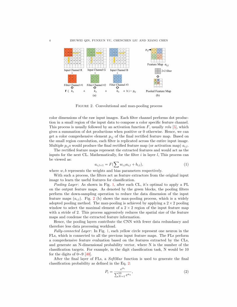
color dimensions of the raw input images. Each filter channel performs dot produc-tion in a small region of the input data to compose a color specific feature channel.This process is usually followed by an activation function F , usually relu [5], whichgives a summation of dot productions when positive or 0 otherwise. Hence, we canget a color comprehensive element pij of the final rectified feature map. Based onthe small region convolution, each filter is replicated across the entire input image.Multiple pijs would produce the final rectified feature map (or activation map) ai,l.

The rectified feature maps represent the extracted features and would act as theinputs for the next CL. Mathematically, for the filter i in layer l, This process canbe viewed as:

ai,l+1 = F (∑

wi,lai,l + bi,l), (1)

where w, b represents the weights and bias parameters respectively.With such a process, the filters act as feature extractors from the original input

image to learn the useful features for classification.Pooling Layer : As shown in Fig. 1, after each CL, it’s optimal to apply a PL

on the output feature maps. As denoted by the green blocks, the pooling filtersperform the down-sampling operation to reduce the data dimension of the inputfeature maps (ai,l). Fig. 2 (b) shows the max-pooling process, which is a widelyadopted pooling method. The max-pooling is achieved by applying a 2× 2 poolingwindow to select the maximal element of a 2 × 2 region of the input feature mapwith a stride of 2. This process aggressively reduces the spatial size of the featuremaps and condense the extracted feature information.

Hence, the pooling layers contribute the CNN with fewer data redundancy andtherefore less data processing workload.

Fully-connected Layer : In Fig. 1, each yellow circle represent one neuron in theFLs, which is connected to all the previous input feature maps. The FLs performa comprehensive feature evaluation based on the features extracted by the CLs,and generate an N-dimensional probability vector, where N is the number of theclassification targets. For example, in the digit classification task, N would be 10for the digits of 0∼9 [40].

After the final layer of FLs, a SoftMax function is used to generate the finalclassification probability as defined in the Eq. 2:

Pi =eai∑10N=1 e

an, (2)


where ai is ith neuron output in the final FL layer. This function normalizes thefinal FL layer output to a vector of values between zero and one, which gives aprobability over all 10 classes.

By applying the above-mentioned hierarchical structured layers, CNNs transformthe input image layer by layer from the original pixel values to the final probabilityvector P , in which the largest Pi indicates the most predicted class.

2.2. CNN algorithm. The CNNs not only benefit from the deep hierarchicalstructure, but also the delicate learning algorithm [39]. The learning algorithmaims to minimize the training error between the predicted values and actual labelsby updating the network parameters, which are quantified by the loss function. Thetraining error can be viewed as:

C(w, b) =1

n

i=1∑n

L(w, b, xi, yi), (3)

where L(·) represents the loss function, and (x1, y1), ...(xn, yn) represent the trainingexamples. During the learning process, a square loss is usually applied, then theloss function will be:

L(w, b, xi, yi) = (yi − f(w, b, xi))2, (4)

where f(·) indicates the predicted values calculated by the whole CNN:

f(w, b, x) = F (∑

wi,lF (wi,l−1F (...F (∑

wi,1xi,0 + bi,0)...) + bi,l−1) + bi,l). (5)

In order to minimize the C(w, b), a partial derivative ∂C/∂(w, b) with respect toeach weight w and bias b is calculated by backpropagating through all the layers inthe CNN. The gradient descent method is utilized to iteratively update all parametervalues. The update procedure for w from iteration j to j + 1 can be viewed as:

wj+1 = wj − η ·∂C(w;x, y)

∂w, (6)

where η is the learning rate. Before the learning process, the parameters are usu-ally randomly initialized [21]. With the learning process, the convolutional filtersbecome well configured to extract certain features. The features captured by con-volutional filters can be demonstrated by visualization.

A lot of works have been proposed to optimize the structure and algorithm ofthe CNNs. For example, much deeper network structures have been investigated,such as VGG, GoogleNet, and ResNet. At the same time, some regularization andoptimization techniques have been applied, such as dropout [65], batch normaliza-tion [31], momentum [56], and adagrad [13]. As a result, CNNs have been welloptimized and widely used in computer vision related tasks. However, the CNNsstill suffer from high computational cost, slow training speed, and large trainingdataset requirement, which highly compromise the applicability and performanceefficiency [26]. Hence, these weakness require more understanding about the CNNworking mechanism to further optimize the CNN.

2.3. CNN visualization mechanism. CNN visualization is a well utilized quali-tative method to analysis the CNN working mechanism regarding the network inter-pretability. The interpretability is related to the ability of the human to understandthe CNNs, which can be improved by demonstrating the internal features learnedby CNNs. Visualization greatly helps to interpret the CNN’s internal features, sinceit utilizes the human visual cortex system as a reference.


edgeslines

shapesobjectsfaces

Input image

1st CL

2nd CL

3rd CL

1th FL

2nd FL

V1

V2

V4

IT

Edges Lines

Objects

Shapes

Face

Human Vision CNNs Visualization

CLs

FLs

Figure 3. Human vision and CNNs visualization

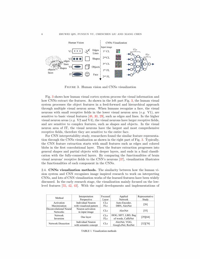
Fig. 3 shows how human visual cortex system process the visual information andhow CNNs extract the features. As shown in the left part Fig. 3, the human visualsystem processes the object features in a feed-forward and hierarchical approachthrough multiple visual neuron areas. When humans recognize a face, the visualneurons with small receptive fields in the lower visual neuron area (e.g. V1), aresensitive to basic visual features [48, 30, 29], such as edges and lines. In the highervisual neuron areas (e.g. V2 and V4), the visual neurons have larger receptive fields,and are sensitive to complex features, such as shapes and objects. In the visualneuron area of IT, the visual neurons have the largest and most comprehensivereceptive fields, therefore they are sensitive to the entire face.

For CNN interpretability study, researchers found the similar feature representa-tion through the CNNs visualization as shown in the right part of Fig. 3. Typically,the CNN feature extraction starts with small features such as edges and coloredblobs in the first convolutional layer. Then the feature extraction progresses intogeneral shapes and partial objects with deeper layers, and ends in a final classifi-cation with the fully-connected layers. By comparing the functionalities of brainvisual neurons’ receptive fields to the CNN’s neurons [37], visualization illustratesthe functionalities of each component in the CNNs.

2.4. CNNs visualization methods. The similarity between how the human vi-sion system and CNN recognizes image inspired research to work on interpretingCNNs, and lots of CNN visualization works of the learned features have been widelydiscussed. In the early research stage, the visualization mainly focused on the low-level features [55, 42, 43]. With the rapid developments and implementations of

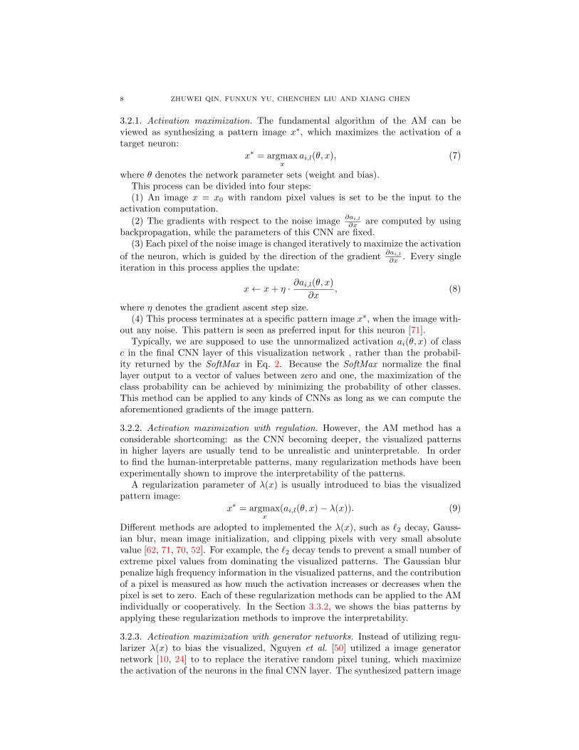
Method InterpretationPerspective

FocusedLayer

AppliedNetwork

Representative Study

Activation Maximization

Individual Neuronwith visualized pattern

CLsFLs

Auto-Encoder, DBN, AlexNet [26]

Deconvolutional Neural Networks

Neuron activation in input image CLs AlexNet [55]

NetworkInversion One layer CLs

FLsHOG, SIFT, LBD, Bag

of words, CaffeNet [29][64]

Network Dissection Individual Neuronwith semantic concept CLs AlexNet, VGG,

GoogLeNet, ResNet [32][70]

TABLE 1. Visualization methods


CNNs, the visualization has been extended to interpret the overall working mecha-nism of CNNs. In Table 1, we give a brief review of four representative visualizationmethods, namely Activation Maximization, Deconvolutional Networks (DeconNet),Network Inversion, and Network Dissection:

• In Activation Maximization, a visualized input image pattern is synthesized toillustrate a specific neuron’s max stimulus in each layer;

• DeconNet utilizes an inversed CNN structure, which is composed deconvolu-tional and unpooling layers, to find the image pattern in the original input imagefor a specific neuron activation;

• Network Inversion reconstructs an input image based on the original imagefrom a specific layer’s feature maps, which reveals what image information is pre-served in that layer;

• Network Dissection describes neurons as visual semantic detectors, which canmatch six kinds of semantic concepts (e.g. scene, object, part, material, texture,and color).

To compare these methods directly, we summarize the overview, algorithms, andvisualization results of these methods: 1) The overview summarizes the history andrepresent works in this line of work. 2) The algorithms explain how this methodworks for the CNNs visualization. 3) The visualization results provide a compre-hensive understanding how CNNs extract features.

3. Visualization by activation maximization.

Synthesize an input pattern image that can maximize a specific neuron’s activa-tion in arbitrary layers.

3.1. The overview. Activation Maximization (AM) is proposed to visualize thepreferred inputs of neurons in each layer. The preferred input can indicate whatfeatures of a neuron has learned. The learned feature is represented by a synthesizedinput pattern that can cause maximal activation of a neuron. In order to synthesizesuch an input pattern, each pixel of the CNN’s input is iteratively changed tomaximize the activation of the neuron.

The idea behind the AM is intuitive, and the fundamental algorithm was pro-posed by Erhan et al. in 2009 [14]. They visualized the preferred input patterns forthe hidden neurons in the Deep Belief Net [28] and the Stacked Denoising Auto-Encoder [68] learned from the MNIST digit dataset [40]. Later, Simonyan et al.utilized this method to maximize the activation of neurons in the last layer ofCNNs [62]. Google also has synthesized similar visualized patterns for their incep-tion network [49]. Yosinksi et al. further applied the AM in a large scale, whichvisualized the arbitrary neurons in all layers of a CNN [71]. Recently, a lot of opti-mization works have followed this idea to improve the interpretability and diversityof the visualized patterns [52, 50]. With all these works, the AM has demonstratedgreat capability to interpret the interests of neurons and identify the hierarchicalfeatures learned by CNNs.

3.2. The algorithm. In this section, the fundamental algorithm of the AM ispresented. Then, another optimized AM algorithm is discussed, which dramaticallyimproves the interpretability of visualized patterns by utilizing a deep generatornetwork [50].


3.2.1. Activation maximization. The fundamental algorithm of the AM can beviewed as synthesizing a pattern image x∗, which maximizes the activation of atarget neuron:

x∗ = argmaxx

ai,l(θ, x), (7)

where θ denotes the network parameter sets (weight and bias).This process can be divided into four steps:(1) An image x = x0 with random pixel values is set to be the input to the

activation computation.

(2) The gradients with respect to the noise image∂ai,l∂x are computed by using

backpropagation, while the parameters of this CNN are fixed.(3) Each pixel of the noise image is changed iteratively to maximize the activation

of the neuron, which is guided by the direction of the gradient∂ai,l∂x . Every single

iteration in this process applies the update:

x← x+ η · ∂ai,l(θ, x)

∂x, (8)

where η denotes the gradient ascent step size.(4) This process terminates at a specific pattern image x∗, when the image with-

out any noise. This pattern is seen as preferred input for this neuron [71].Typically, we are supposed to use the unnormalized activation ai(θ, x) of class

c in the final CNN layer of this visualization network , rather than the probabil-ity returned by the SoftMax in Eq. 2. Because the SoftMax normalize the finallayer output to a vector of values between zero and one, the maximization of theclass probability can be achieved by minimizing the probability of other classes.This method can be applied to any kinds of CNNs as long as we can compute theaforementioned gradients of the image pattern.

3.2.2. Activation maximization with regulation. However, the AM method has aconsiderable shortcoming: as the CNN becoming deeper, the visualized patternsin higher layers are usually tend to be unrealistic and uninterpretable. In orderto find the human-interpretable patterns, many regularization methods have beenexperimentally shown to improve the interpretability of the patterns.

A regularization parameter of λ(x) is usually introduced to bias the visualizedpattern image:

x∗ = argmaxx

(ai,l(θ, x)− λ(x)). (9)

Different methods are adopted to implemented the λ(x), such as `2 decay, Gauss-ian blur, mean image initialization, and clipping pixels with very small absolutevalue [62, 71, 70, 52]. For example, the `2 decay tends to prevent a small number ofextreme pixel values from dominating the visualized patterns. The Gaussian blurpenalize high frequency information in the visualized patterns, and the contributionof a pixel is measured as how much the activation increases or decreases when thepixel is set to zero. Each of these regularization methods can be applied to the AMindividually or cooperatively. In the Section 3.3.2, we shows the bias patterns byapplying these regularization methods to improve the interpretability.

3.2.3. Activation maximization with generator networks. Instead of utilizing regu-larizer λ(x) to bias the visualized, Nguyen et al. [50] utilized a image generatornetwork [10, 24] to to replace the iterative random pixel tuning, which maximizethe activation of the neurons in the final CNN layer. The synthesized pattern image


by the generator is more close to the realistic image, which greatly improves theinterpretability of the visualized patterns.

Recently, most of the generator networks related works are based on GenerativeAdversarial Networks (GAN) [24]. GANs can learn to mimic any distribution ofdata and generate realistic data samples, such as image, music, and speech, which isfeatured with a complementary composition of two neural networks: One generativenetwork takes noise as input and aim to generate realistic data samples. Anotherdiscriminator network receives the generated data samples from the output of thegenerative network and the real data samples from the training data sets, whichaim to distinguishes between the two sources. The goal of generative network isto generate passable data samples, to lie without being distinguished by the dis-criminator network. The goal of the discriminator is to identify images comingfrom the generative network as fake. After fine training of both the networks, theGAN eventually achieves a balance, where the discriminator can hardly distinguishgenerated data samples from real data samples. In such a case, we can claim thatthe generative network has achieved an optimal capability in generating realisticsamples. So far GANs have particularly produced excellent results in image data,and primarily been used to generate samples of realistic images [9, 41, 2].

Benefit from the success of GANs, the generative network is utilized to overcomethe aforementioned shortcoming of AM that the visualized patterns in higher layersare usually tend to be unrealistic and uninterpretable. The generative network isutilized to generate or synthesize the pattern image that maximize the activationof the selected neuron ai,l in the final layer This method is called Deep GenerativeNetwork Activation Maximization (DGN-AM).

The DGN-AM implemention can be view as:

x∗ = argmaxx

(ai,l(θ,G(x))− λ(x)), (10)

where G indicates the generative network that takes the noise image as input. Itcan synthesize the pattern image that causes high activation of the target neuronai,l. In [50], the author found that the `2 regularization with small degree helps togenerate more human-interpretable patterns. In the Section 3.3.3, we compare thepattern image synthesized by the AM and DGN-AM.

3.3. Experiments with activation maximization. In this section, the experi-ments of AM on CaffeNet trained with ImageNet dataset are demonstrated, whichshows what features have been learned by each neuron. The first layer neuronscan be visualized by directly mapping each filter matrix to an RGB pattern image,hence, the first layer visualization by AM and the direct mapping method are eval-uated to show the effectiveness of AM. Then the hidden layer visualization showsthe abundant and hierarchical features learned by different layer neurons. Finallythe final layer visualization by AM and DGN-AM are compared to emphasize theimprovement of interpretability by the DGN-AM.

3.3.1. First layer visualization. As aforementioned, the AM has more distinguish-able performance on the early network layers, hence, we first evaluate the first layervisualization with AM.

Fig. 4 (a) shows several visualization results of synthesizing the patterns for four

different neurons. This process uses the gradient∂ai,l∂x to tweak the input noise

iteratively, which increases the activation of neuron i. After 400 iterations, we


1

𝑥0 Iterations 20 40 100 400

Gradient

Ascent

Activation Maximization (400) Direct Map

(a)

(b)

Figure 4. First layer of CaffeNet visualized by Activation Maximization

can get relatively smooth visualized patterns, which indicates a nicely convergednetwork is trained.

Fig. 4 (b) shows the visualized patterns synthesized by the AM and direct map-ping method. As we can see, most of the visualized patterns synthesized by theAM are almost the same as the corresponding direct mapped patterns. The vi-sualized patterns are clustered into two groups: 1) the colorful patterns indicatethe corresponding neurons greatly sensitive to color components in the under-testimages; 2) the black-and-white patterns indicate the corresponding neurons greatlysensitive to shape information. In addition, through comparison with the directmap method, the AM can reveal the preferred inputs of each neuron accurately.

This interesting finding reveals that the CNNs attempt to imitate the humanvisual cortex system, which the neurons in the lower visual area are sensitive tobasic patterns, such as colors, edges, and lines.

3.3.2. Hidden layers visualization. Beyond the first layer, the neurons in the fol-lowing layers gradually learn to extract feature hierarchically.

Fig. 5 shows the visualization of 6 hidden layers from the second convolutionallayer (CL 2) to the second fully connected layer (FL 2) in each row. Several neuronsin each layer are randomly selected as our AM test targets. We observed that: 1)Some important patterns are visualized, such as edges (CL 2-4), faces (CL 4-1),wheels (CL 4-2), bottles (CL 5-1), eyes (CL 5-2), etc., which demonstrate the abun-dant features learned by the neurons. 2) Meanwhile, not all the visualized patternsare interpretable even with multiple regularization methods are applied. 3) Thecomplexity and variation of the visualized patterns are increasing from lower layersto higher layers, which indicates that increasingly invariant features are learned bythe neurons. 4) From the CL 5 to FLs, we can find there is a large pattern varia-tion increment, which could indicate the FLs provide a more comprehensive featureevaluation.

3.3.3. Final layer visualization. The final layer of the CaffeNet contains 1000 neu-rons, which corresponding to the 1000 classes in the ImageNet dataset. Five differ-ent neurons are selected to show the visualized pattern image.


CL 2

CL 3

CL 4

CL 5

FL 1

FL 2

Figure 5. Hidden layers of CaffeNet visualization by Activation Maximization.Adapted from “Understanding Neural Networks Through Deep Visualization,” by

J. Yosinski, 2015.

Fig. 6 compares the visualized patterns synthesized by the AM and the DGN-AM for five different classes in FL 3. For the AM shown in the first row of Fig. 6,although we can guess which class the visualized patterns represents, there aremultiple duplicate and vague objects in the each visualized pattern, such as three

846: table lamp487: cell phone462: broom 629: lipstick 899: water jug

AM

DGN

-

AM

Figure 6. Output layer of CaffeNet visualized by Activation Maximization.


lipsticks in the third column (AM-3) and the images are far from being photo-realistic. For the DGN-AM shown in the second row of Fig. 6, by utilizing thegenerator networks, the DGN-AM greatly improves the images quality in termsof color and texture. Because the fully connected layer contain information fromall areas of the image and the generator network provides a strong biases towardrealistic visualizations.

Through the final layer visualization, we can clearly see what objects combina-tions could affect the CNN classification decision. For example, if the CNN classifiesan image of a cell phone held in a human hand as a cell phone, it is unclear if theclassification decision is affected by the human hand. Through the visualization,we can see there is a cell phone and a human hand in the cell phone class, whichare shown in the second row and third column. In this case, the visualization showsthe CNN has learned to detect both object information in one image.

3.4. The summary. As the most intuitive visualization method, the AM revealsthat CNNs learn to detect the important features such as faces, wheels, and bottleswithout our specification. At the same time, CNNs attempt to mimic the hierarchi-cal organization of the visual cortex, and then successfully build up the hierarchicalfeature extraction. In addition, this visualization method suggests that the individ-ual neurons extract features in a more local manner rather than distributed, whicheach neuron correspond to a specific pattern.

4. Visualization by deconvolutional network.

Find the selective pattern from a given input image that activate a specific neuronin the convolutional layers.

4.1. The overview. While the Activation Maximization interprets the CNNs fromthe perspective of the neurons, the Deconvolutional Network (DeconvNet) basedCNN visualization explains the CNNs from the perspective of the input image. Itfinds the selective patterns from the input image that activate a specific neuronin the convolutional layers. The patterns are reconstructed by projecting the low-dimension neurons’ feature maps back to the image dimension. This projectionprocess is implemented by a DeconvNet structure, which contains deconvolutionallayers and unpooling layers, performing the inversed computation of the convolu-tional and pooling layers. Rather than purely analyzing the neurons’ interests, theDeconvNet based visualization demonstrates a straightforward feature analysis inan image level.

The research related to the DeconvNet structure is mainly led by Zeiler et al.In [73], they first proposed the DeconvNet structure aiming to capture certain gen-eral features for reconstructing the natural image by projecting a highly diverseset of low-dimension feature maps to high dimension. Later in [74], they utilizedthe DeconvNet structure to decompose an image hierarchically, which could cap-ture the image information at all scales, from low-level edges to high-level objectparts. Eventually, they applied the DeconvNet structure for CNN visualization byinterpreting CNN hidden features [72], which made it become an effective methodto visualize the CNNs.

4.2. The algorithm. The DeconvNet is an effective method to visualize the CNNs,we will explain the DeconvNet based visualization in terms of DeconvNet structureand the visualization process in this section.


fRelu

Un

poolin

g

Reluf T

2 4 3 6 …

6 8 9 4 …

2 5 6 9 …

7 0 10 7 …

… … … … …

Rectified

Feature Map

8 9 …7 10 …… … …

Pooled Feature Map

…

M M …

…

M M …

… … … … …

0 0 0 0 …

0 8 9 0 …

0 0 0 0 …

7 0 10 0 …

… … … … …

Unpooled

Feature Map

Switches

𝐴𝑙

𝐴𝑙+1 𝐴𝑙+1𝑟

𝐴𝑙+1𝑝

𝑅𝑙+1𝑅𝑙

Switches

(a) (b)

deco

nvn

etco

nvn

et

𝑅𝑙+1𝑢𝑝

Figure 7. The structure of the Deconvolutional Network

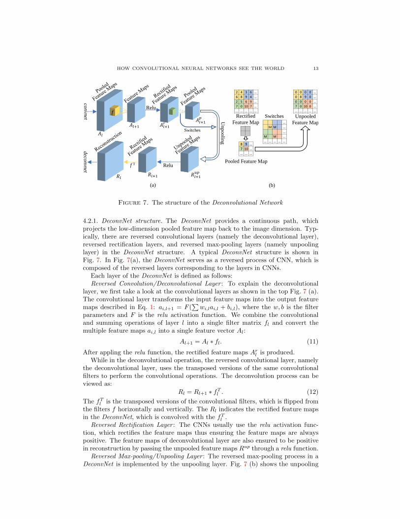
4.2.1. DeconvNet structure. The DeconvNet provides a continuous path, whichprojects the low-dimension pooled feature map back to the image dimension. Typ-ically, there are reversed convolutional layers (namely the deconvolutional layer),reversed rectification layers, and reversed max-pooling layers (namely unpoolinglayer) in the DeconvNet structure. A typical DeconvNet structure is shown inFig. 7. In Fig. 7(a), the DeconvNet serves as a reversed process of CNN, which iscomposed of the reversed layers corresponding to the layers in CNNs.

Each layer of the DeconvNet is defined as follows:Reversed Convolution/Deconvolutional Layer : To explain the deconvolutional

layer, we first take a look at the convolutional layers as shown in the top Fig. 7 (a).The convolutional layer transforms the input feature maps into the output featuremaps described in Eq. 1: ai,l+1 = F (

∑wi,lai,l + bi,l), where the w, b is the filter

parameters and F is the relu activation function. We combine the convolutionaland summing operations of layer l into a single filter matrix fl and convert themultiple feature maps ai,l into a single feature vector Al:

Al+1 = Al ∗ fl. (11)

After appling the relu function, the rectified feature maps Arl is produced.While in the deconvolutional operation, the reversed convolutional layer, namely

the deconvolutional layer, uses the transposed versions of the same convolutionalfilters to perform the convolutional operations. The deconvolution process can beviewed as:

Rl = Rl+1 ∗ fTl . (12)

The fTl is the transposed versions of the convolutional filters, which is flipped fromthe filters f horizontally and vertically. The Rl indicates the rectified feature mapsin the DeconvNet, which is convolved with the fTl .

Reversed Rectification Layer : The CNNs usually use the relu activation func-tion, which rectifies the feature maps thus ensuring the feature maps are alwayspositive. The feature maps of deconvolutional layer are also ensured to be positivein reconstruction by passing the unpooled feature maps Rup through a relu function.

Reversed Max-pooling/Unpooling Layer : The reversed max-pooling process in aDeconvNet is implemented by the unpooling layer. Fig. 7 (b) shows the unpooling


process in detail: In order to implement the reversed operation of max-pooling,which performs the downsampling operation on the rectified feature maps Arl+1,the unpooling layer transform the pooled feature maps to the unpooled featuremaps.

During the max-pooling operation, the positions of maximal values within eachpooling window are recorded in switch variables. The switches first specify the posi-tion of which elements in the rectified feature map are copied into the pooled featuremap, then mark them as M in the switches. These switches variables are used inthe unpooling operation to place each maximal value back to its original pooledlocation. Due to the dimension gap, certain amount of locations are inevitable con-structed without certain information, therefore these locations are usually filled byzero for compensation.

4.2.2. Visualization process. Based on the reversed structure formed by those layers,the DeconvNet can be well utilized to visualize the CNNs. The visualization processcan be described as follows:

(1) All neurons’ feature maps can be captured when a specific input image isprocessed through the CNN.

(2) The feature map of the target neuron for visualization is selected while allother neurons’ feature maps are set to zeros.

(3) In order to obtain the visualized pattern, the target neuron’s feature map isprojected back to the image dimension through the DeconvNet.

(4) To visualize all the neurons, this process is applied to all neurons repeatedlyand obtain a set of corresponding pattern images for CNN visualization.

These visualized patterns indicate which pixels or features in the input imagecontribute to the activation of the neuron, and it also can be used to examine theCNN design shortcomings. In the next section, these visualized patterns will bedemonstrated with practical experiements.

4.3. Experiments with DeconvNet based visualization. In this section, theexperiments of DeconvNet based visualization on CaffeNet trained with ImageNetdataset are demonstrated, to show what features have been learned by each neuron.In addition, this method can be used as an efficient tools for network analysis,optimization and training monitoring.

4.3.1. Convolutional layer visualization. As aforementioned, the DeconvNet struc-ture provides a continuous path back to the image dimension, which can highlightspecific pattern in the input image that excites a neuron.

1CL 1 CL 2 CL 3 CL 4 CL 5

Figure 8. CaffeNet visualized by DeconvNet


Fig. 8 shows the DeconvNet based visualization examples with 5 convolutionallayers of the CaffeNet from CL1 to CL5. In each layer, we randomly select twoneurons’ visualized patterns comparing to the corresponding local sections in theoriginal image. From these examples, we can tell that: Each individual neuronextracts feature in a more local manner, where different neurons in one layer areresponsible for different patterns, such as mouth, eyes, and ears.

Lower layers (CL1, CL 2) capture the small edges, corners, and parts. CL3 hasmore complex invariance, capturing similar textures such as mesh patterns. Higherlayers (CL4, CL5) are more class-specific, which show the almost entire objects.Compared to the Activation Maximization, the DeconvNet based visualization canprovide much more explicit and straightforward patterns.

4.3.2. DeconvNet based visualization for network analysis and optimization. Besidethe convolutional layer visualization for interpretation analysis, DeconvNet can bealso used to examine the CNN design for further optimization.

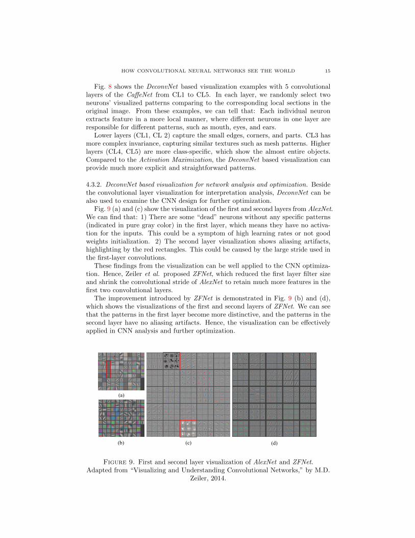
Fig. 9 (a) and (c) show the visualization of the first and second layers from AlexNet.We can find that: 1) There are some “dead” neurons without any specific patterns(indicated in pure gray color) in the first layer, which means they have no activa-tion for the inputs. This could be a symptom of high learning rates or not goodweights initialization. 2) The second layer visualization shows aliasing artifacts,highlighting by the red rectangles. This could be caused by the large stride used inthe first-layer convolutions.

These findings from the visualization can be well applied to the CNN optimiza-tion. Hence, Zeiler et al. proposed ZFNet, which reduced the first layer filter sizeand shrink the convolutional stride of AlexNet to retain much more features in thefirst two convolutional layers.

The improvement introduced by ZFNet is demonstrated in Fig. 9 (b) and (d),which shows the visualizations of the first and second layers of ZFNet. We can seethat the patterns in the first layer become more distinctive, and the patterns in thesecond layer have no aliasing artifacts. Hence, the visualization can be effectivelyapplied in CNN analysis and further optimization.

(a)

(b) (c) (d)

Figure 9. First and second layer visualization of AlexNet and ZFNet.Adapted from “Visualizing and Understanding Convolutional Networks,” by M.D.

Zeiler, 2014.


1CL 1 CL 2 CL 3 CL 4 CL 5 1 2 5 10 20 30 40 64 1 2 5 10 20 30 40 64 1 2 5 10 20 30 40 64 1 2 5 10 20 30 40 64 1 2 5 10 20 30 40 64

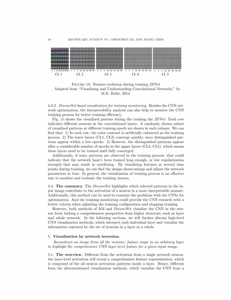
Figure 10. Feature evolution during training ZFNet. Adapted from “Visualizing and Understanding Convolutional Networks,” by

M.D. Zeiler, 2014.

4.3.3. DeconvNet based visualization for training monitoring. Besides the CNN net-work optimization, the interpretability analysis can also help to monitor the CNNtraining process for better training efficiency.

Fig. 10 shows the visualized pattens during the training the ZFNet. Each rowindicates different neurons in the convolutional layers. A randomly chosen subsetof visualized patterns at different training epoch are shown in each column. We canfind that: 1) In each row, the color contrast is artificially enhanced as the trainingprocess. 2) The lower layers (CL1, CL2) converge quickly, since distinguished pat-terns appear within a few epochs. 3) However, the distinguished patterns appearafter a considerable number of epochs in the upper layers (CL4, CL5), which meansthese layers need to be trained until fully converged.

Additionally, if noisy patterns are observed in the training process, that couldindicate that the network hasn’t been trained long enough, or low regularizationstrength that may result in overfitting. By visualizing features at several timepoints during training, we can find the design shortcomings and adjust the networkparameters in time. In general, the visualization of training process is an effectiveway to monitor and evaluate the training statues.

4.4. The summary. The DeconvNet highlights which selected patterns in the in-put image contribute to the activation of a neuron in a more interpretable manner.Additionally, this method can be used to examine the problems with the CNNs foroptimization. And the training monitoring could provide the CNN research with abetter criteria when adjusting the training configuration and stopping training.

However, both methods of AM and DeconvNet visualize the CNN in the neu-ron level, lacking a comprehensive perspective from higher structure, such as layerand whole network. In the following sections, we will further discuss high-levelCNN visualization methods, which interpret each individual layer and visualize theinformation captured by the set of neurons in a layer as a whole.

5. Visualization by network inversion.

Reconstruct an image from all the neurons’ feature maps in an arbitrary layerto highlight the comprehensive CNN layer-level feature for a given input image.

5.1. The overview. Different from the activation from a single network neuron,the layer-level activation will reveal a comprehensive feature representation, whichis composed of the all neuron activation patterns inside a layer. Hence, differentform the aforementioned visualization methods, which visualize the CNN from a


single neuron’s activation, the Network Inversion based visualization can be usedto analysis the activation information from a layer level perspective.

Before the Network Inversion is applied to visualize the CNNs, the fundamentalidea of Network Inversion was proposed to study the traditional computer visionrepresentation, such as the Histogram of Oriented Gradients (HOG) [7, 15, 19],the Scale Invariant Feature Transform (SIFT) [45], the Local Binary Descriptors(LBD) [8], and the Bag of Visual Words Descriptors [6, 64]. Later, two variants ofthe Network Inversion were proposed for CNN visualization [46, 47, 11]:

(1) Regularizer based Network Inversion: It is proposed by Mahendran et al.,which reconstructs the image from each layer by using gradient descent approachand a regularization term [46, 47].

(2) UpconvNet based Network Inversion: It is proposed by Dosovitskiy et al. [11,12], which reconstructs the image by training a dedicated Up-convolutional NeuralNetwork (UpconvNet).

Overall, the main goal of both algorithms is to reconstruct the original inputimage from one whole layer’s feature maps’ specific activation. The Regularizerbased Network Inversion is easier to be implemented, since it does not require totrain an extra dedicated network. While the UpconvNet based Network Inversioncan visualize more existent information in higher layers with an extra dedicatednetwork and significantly more computational cost.

5.2. The algorithm. In this section, we compared the aforementioned two Net-work Inversion based Visualization methods regarding the network structure andthe learning algorithm.

Fig. 11 shows the network implementation for the two Network Inversion basedVisualization methods comparing with the original CNN: the Regularizer basedNetwork Inversion is shown in the upper as denoted in green, and the UpconvNetbased Network Inversion is shown in the bottom as denoted in orange, while theoriginal CNN is shown in the middle as denoted in blue.

The Regularizer based Network Inversion has the same architecture and param-eters as the original CNN before the visualization target layer. In this case, eachpixel of the to be reconstructed image x0 is adjusted to minimize the objective lossfunction error between the target feature map A(x0) of x0 and the feature mapA(x) of the original input image x.

For the UpconvNet based Network Inversion, the UpconvNet provides a inversepath for the feature map back to the image dimension. The parameters of theUpconvNet are adjusted to minimize the objective loss function error between thereconstructed image x0 and the original input image x.

In the following sections, we will give detailed explanations of the two methodsmathematically.

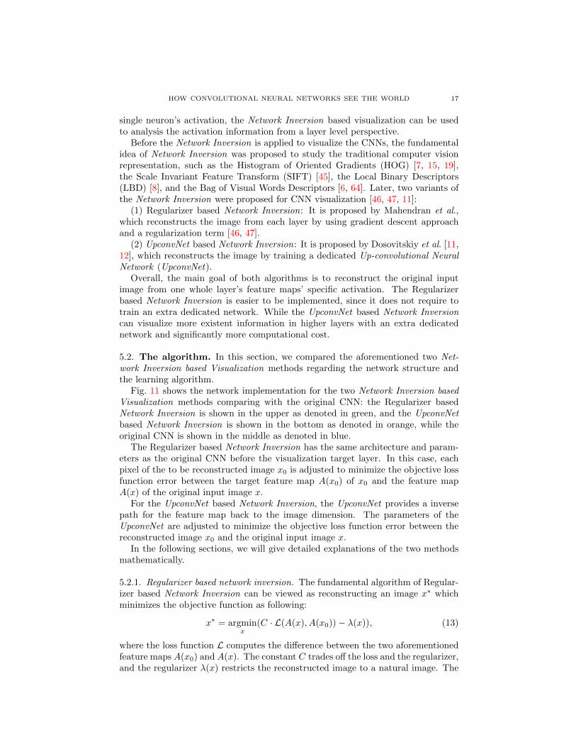
5.2.1. Regularizer based network inversion. The fundamental algorithm of Regular-izer based Network Inversion can be viewed as reconstructing an image x∗ whichminimizes the objective function as following:

x∗ = argminx

(C · L(A(x), A(x0))− λ(x)), (13)

where the loss function L computes the difference between the two aforementionedfeature maps A(x0) and A(x). The constant C trades off the loss and the regularizer,and the regularizer λ(x) restricts the reconstructed image to a natural image. The


1st CL 1st PL 4th CL 5th CL 1th FL

Loss

1st CL 1st PL 4th CL 5th CL

Loss

OriginalC

NN

upconvnet

upconvnet

InversionW

ith Regularizer

InversionW

ith UpconvN

et

A(x)

A(x0)

x

x0

x0

Figure 11. The data flow of the two Network Inversion algorithms

loss function is usually defined as a Euclidean distance:

L(A(x), A(x0)) = ‖A(x)−A(x0)‖2 , (14)

which is the most commonly used measurement to evaluate the similarity betweendifferent images [69].

In order to make the reconstructed images look closer to the nature images,multiple regularization approaches have been experimentally studied to improvethe reconstruction quality, such as α-norm, total variation norm (TV) , jittering,and texture or style regularizers [59, 49, 18]. As an example, for a discrete imagedata x ⊂ RHXW , the TV norm is given by:

λ(x) =∑i,j

((xi,j+1 − xi,j)2 + (xi+1,j − xi,j)2)β2 , (15)

where the regularizer β =1 stands for the standard TV norm that is mostly usedin image denoising. In this case, the TV norm penalizes the reconstructed imagesto encourage the spatial smoothness.

Based on such a Network Inversion framework, the visualization process can bedivided into five steps:

(1) The visualization target layer’s feature maps A(x) of the original input imagex and the feature maps A(x0) of the to be reconstructed x0 (initialized with noise)are firstly computed.

(2) The error between the two feature map sets – L(A(x), A(x0)) is then com-puted by the objective loss function.

(3) Guided by the direction of the gradient L(A(x),A(x0))∂x , each pixel of the noise

image is changed iteratively to minimize the objective loss function error.(4) This process terminates at a specific reconstructed image x∗, which is used

to demonstrate what information is preserve in the visualization target layer.The Regularizer based Network Inversion iteratively tweaks the input noise to-

wards the direction that minimizes the difference between the two feature map sets,while the UpconvNet based Network Inversion minimizes the image reconstructionerror. In the next section, we will then discuss the UpconvNet based Network In-version in detail.


5.2.2. UpconvNet based network inversion. Although the Regularizer based NetworkInversion can reconstruct a image for CNN layer visualization, it still suffer fromrelatively slow computation speed due to gradient computation. To overcome thisshortcoming, Dosovitskiy et al. proposed another Network Inversion approach,which trained an extra dedicated Up-convolutional Neural Network (UpconvNet) toreconstruct the image with better image quality and computation efficiency [11].

The UpconvNet can project the low-dimension feature maps back to the imagedimension with similar reversed layers as in DeconvNet. As shown in the bottompart of Fig. 11, the UpconvNet takes the feature maps A(x) as the input, and yieldsthe reconstructed image as the output.

Each layer of the UpconvNet are described as follows:Reversed Convolutional Layer : The filters are re-trained in the UpconvNet whereas

the DeconvNet uses the transposed versions of the same convolutional filters. Givena training set of images and their feature maps (xi, A(xi)), the training procedurecan be viewed as:

W ∗ = argminw

∑i

||xi −D(A(xi),W )||2, (16)

where the weight W of UpconvNet is optimized to minimize the squared Euclideandistance between the input image xi and the output of UpconvNet – D(A(xi),W ).

Reversed Rectification Layer : The feature maps of UpconvNet are also ensuredto be positive, with the leaky relu nonlinearity of slope 0.2 is applied:

A(x) =

{x x > 0

0.2 x < 0(17)

Reversed Max-pooling Layer : The unpooling layers in UpconvNet are quite sim-plified. The feature maps are upsampled by a factor of 2, which replaces each valueby a 2 × 2 block with the original value in the top left corner and all other entriesequal to zero.

After the training process, we can utilize this UpconvNet to reconstruct any inputimage without computing the gradients. Therefore, it dramatically decreases thecomputational cost and can be applied to various kinds of deep networks. In the nextsection, we will evaluate the visualization results based on these two approaches.

5.3. Experiments with the network inversion based visualization. In thissection, the experiments of Network Inversion based Visualization is demonstratedbased on AlexNet trained with ImageNet dataset. The experiments demonstratethat Network Inversion based Visualization can not only achieve optimal visualiza-tion performance, but can be also utilized enhance the CNN design.

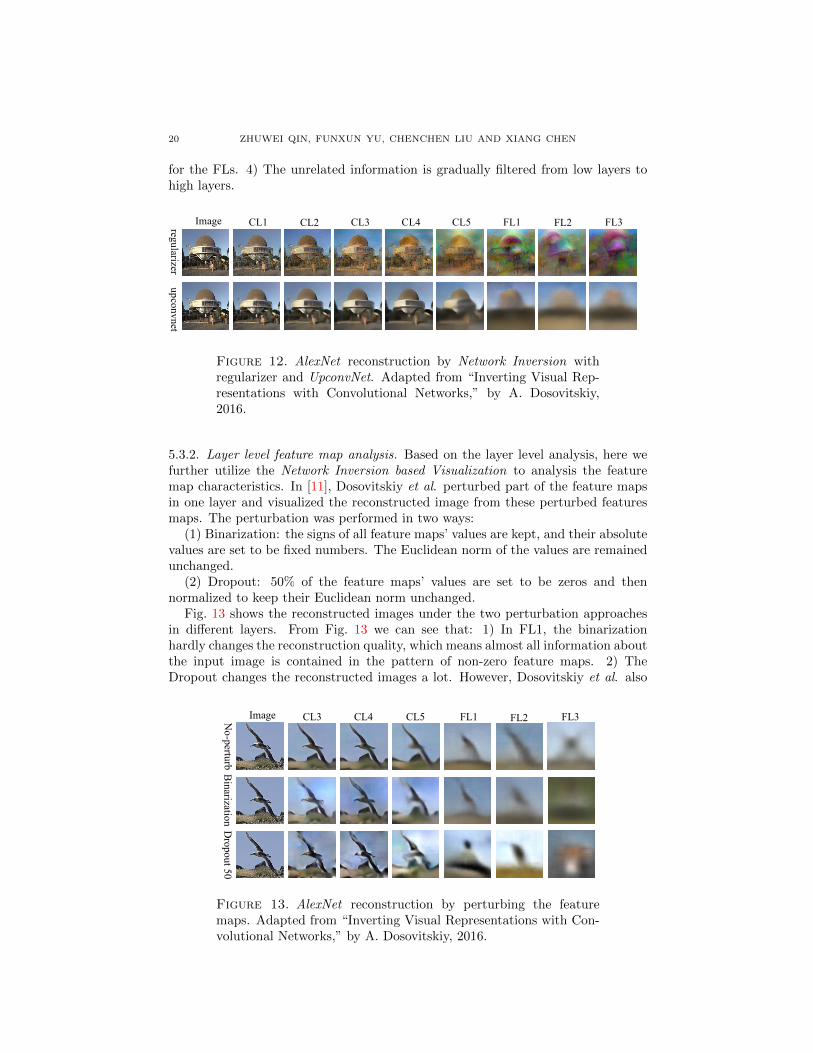
5.3.1. Layer-level visualization analysis. Visualization from layer level can revealwhat features are preserved by each layer. Fig. 12, shows Regularizer and UpconvNetbased visualization from various layers of AlexNet.

From Fig. 12, we can find that: 1) The visualization from the CLs look similarto the original image, although with increasing fuzziness. This indicates that thelower layers preserve much more detailed information, such as colors and locationsof objects. 2) The visualization quality has an obvious drop from the CLs to FLs.However, the visualization from higher CLs and even FLs preserve color (Upcon-vNet) and the approximate object location information. 3) The UpconvNet basedvisualization quality is better than the Regularizer based visualization, especially


for the FLs. 4) The unrelated information is gradually filtered from low layers tohigh layers.

upconvnetregularizer

CL1 CL2 CL3 CL4 CL5 FL1 FL2 FL3Image

Figure 12. AlexNet reconstruction by Network Inversion withregularizer and UpconvNet. Adapted from “Inverting Visual Rep-resentations with Convolutional Networks,” by A. Dosovitskiy,2016.

5.3.2. Layer level feature map analysis. Based on the layer level analysis, here wefurther utilize the Network Inversion based Visualization to analysis the featuremap characteristics. In [11], Dosovitskiy et al. perturbed part of the feature mapsin one layer and visualized the reconstructed image from these perturbed featuresmaps. The perturbation was performed in two ways:

(1) Binarization: the signs of all feature maps’ values are kept, and their absolutevalues are set to be fixed numbers. The Euclidean norm of the values are remainedunchanged.

(2) Dropout: 50% of the feature maps’ values are set to be zeros and thennormalized to keep their Euclidean norm unchanged.

Fig. 13 shows the reconstructed images under the two perturbation approachesin different layers. From Fig. 13 we can see that: 1) In FL1, the binarizationhardly changes the reconstruction quality, which means almost all information aboutthe input image is contained in the pattern of non-zero feature maps. 2) TheDropout changes the reconstructed images a lot. However, Dosovitskiy et al. also

Binarization

No-perturb

CL3 CL4 CL5 FL1 FL2 FL3Image

Dropout 50

Figure 13. AlexNet reconstruction by perturbing the featuremaps. Adapted from “Inverting Visual Representations with Con-volutional Networks,” by A. Dosovitskiy, 2016.


experimentally showed that by Dropouting the 50% least important feature mapscould significantly reduce the reconstruction error, which is even better than notapplying any Dropout for most layers.

These observations could be a proof that various CNN compression techniquescould achieve optimal performance, such as quantization and filter pruning, due tothe considerable amount of redundant information in each layer. Hence the NetworkInversion based Visualization can be used to evaluate the importance of featuremaps, and pruning the least important feature maps for network compression.

5.4. The summary. The Network Inversion based Visualization projects a specificlayer’s feature maps back to the image dimension, which provides insights into whatfeatures a specific layer would preserve. Additionally, by perturbing some featuremaps for visualization, we can verify the CNN preserved a lot redundant informationin each layer, and therefore further optimize the CNN design.

6. Visualization by network dissection.

Evaluate the correlation between each convolutional neuron or multiple neuronswith a specific semantic concept.

6.1. The overview. In previous sections, multiple visualization methods weredemonstrated to reveal the visual perceptible patterns that a single neuron or layercould capture. However, there is still a missing link between the visual perceptiblepatterns and the clear interpretable semantic concepts.

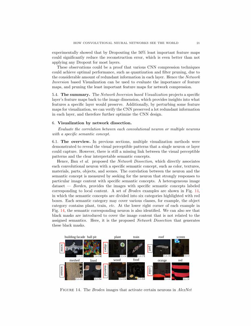
Hence, Bau et al. proposed the Network Dissection, which directly associateseach convolutional neuron with a specific semantic concept, such as color, textures,materials, parts, objects, and scenes. The correlation between the neuron and thesemantic concept is measured by seeking for the neuron that strongly responses toparticular image content with specific semantic concepts. A heterogeneous imagedataset — Borden, provides the images with specific semantic concepts labeledcorresponding to local content. A set of Broden examples are shown in Fig. 14,in which the semantic concepts are divided into six categories highlighted with redboxes. Each semantic category may cover various classes, for example, the objectcategory contains plant, train, etc. At the lower right corner of each example inFig. 14, the semantic corresponding neuron is also identified. We can also see thatblack masks are introduced to cover the image content that is not related to theassigned semantics. Here, it is the proposed Network Dissection that generatesthese black masks.

scene

ob

ject

textu

re

meshed lined

building facade ball pit plant train roof

part

screen

colo

r

orange redwood food

material

CL5-33 CL4-334 CL5-54 CL4-179 CL4-236 CL5-2

CL2-232 CL2-194 CL1-91 CL1-50CL4-254 CL3-202

Figure 14. The Broden images that activate certain neurons in AlexNet


The development of the Network Inversion progressively connects the semanticconcepts to different component levels in a CNN. The fundamental algorithm ofNetwork Inversion illustrated the correlation between one semantic concept andone individual neurons. Such a correlation was based on an assumption that eachsemantic concept can be assigned to a single neuron [23]. Later, further NetworkInversion works revealed that the feature representation can be distributed, whichindicated that one semantic concept could be represented by multiple neurons’ com-bination [1, 75]. Hence, following [3]’s paradigm, Fong et al. proposed another Net-work Inversion approach, namely Net2Vec, which visualized the semantic conceptsbased on neuron combinations [16].

Both methods provide comprehensive visualization results on interpreting CNNhidden neurons.

6.2. The algorithm. In this section, we introduce two Network Dissection meth-ods, one method assigns the semantic concept to each individual neuron, while theother builds the correlation between the neuron combinations and the semanticconcepts.

6.2.1. Network dissection for the individual neuron. The algorithm of Network Dis-section for the individual neuron evaluates the correlation between each single neu-ron and the semantic concept. Specifically, every individual neuron is evaluated asa segmentation task to every semantic concept.

The evaluating process is shown in Fig. 15. The input image fetched from theBroden dataset contains pixel-wise annotations for the semantic concepts, whichprovides the ground truth segmentation masks. The target neuron’s feature mapis upsampled to the resolution of the ground truth segmentation masks. Then theNetwork Dissection works by measuring the alignment between the upsampled neu-ron activation map and the ground truth segmentation masks. If the measurementresult is larger than a threshold, the neuron can be viewed as a visual detector forspecific semantic concept.

This process can be described as follows:

Input image Network being visualized Pixel-wise segmentation

Freeze trained network weights Upsample target feature map Evaluate on segmentation tasks

Figure 15. Illustration of network dissection for measuring se-mantic alignment of neuron in a given CNN. Adapted from “Net-work Dissection: Quantifying Interpretability of Deep Visual Rep-resentations,” by D. Bau, 2017.


(1) The feature map Af (x) of every neuron f is computed by feeding in everyinput image x from Broden. So, the distributions of the activation scores p(ak) ofneuron activation over all images in Broden are computed.

(2) The top activation maps from all feature maps are selected as valid mapregions corresponding to neuron’s semantics by setting an activation threshold thatP (af > Tf ) = 0.005.

(3) To match the low-resolution valid map to the ground truth segmentationmask Lc for some semantic concept c, the valid map is upsampled:

Mf (x) = S(Af (x) > Tf ), (18)

where S denotes a bilinear interpolation function.(4) The accuracy of neuron f in detecting semantic concept c is determined by

the intersection-over-union (IoU) score:

IoUf,c =

∑|Mf (x)

⋂Lc(x)|∑

|Mf (x)⋃Lc(x)|

, (19)

where Lc(x) denotes the ground-truth mask of the semantic concept c on the im-age x. If IoUf,c is larger than a threshold (0.04), we consider the neuron f as avisual detector for concept c. The IoU score indicates the accuracy of neuron f indetecting concept c. Finally, every neuron’s corresponding semantic concept can bedetermined by calculating its IoU score.

Hence, the Network Dissection for the individual neuron can automatically assigna semantic concept to each convolutional neuron.

6.2.2. Network dissection for the neuron combinations. Instead of interpreting theindividual neuron, Fong et al. [16] proposed Net2Vec to evaluate the correlationbetween the neuron combinations and the semantic concepts. They implementedthis approach as a segmentation task by using convolutional neuron combinations.Specifically, a learnable concept weight w is used to linearly combine the thresholdbased activation. And, it is passed through the sigmoid function σ(x) = 1/(1 +exp(−x)) to predict a segmentation mask M(x;w):

M(x;w) = σ(∑k

wk · I(Af (x) > Tf )), (20)

where k is the number of neurons in a layer, and I(·) is the indicator function. Thisfunction selects a subset of neurons in one layer whose activation is larger than thethreshold. Hence, this subset of neurons can be used to generate the activationmask for specific semantic.

Fong et al experimentally found that, for the segmentation task, materials andparts reached near optimal performance around k = 8, which was much more quicklythan that of objects k = 16. For each concept c, the weights w were learnedusing stochastic gradient descent with momentum to minimize per-pixel binarycross entropy loss.

Similar to the single neurons case, the IoUcom score for neuron combinations iscomputed as well:

IoUcom =

∑|Mf,w(x)

⋂Lc(x)|∑

|Mf,w(x)⋃Lc(x)|

. (21)

If the IoUcom score is larger than a threshold, we consider this neuron combinationsas a visual detector for concept c.


CL1 CL2 CL5CL4CL3

red (color) 50 red (color) 197 grass (object) filter 317 water(object) 53 mountain snowy (scene) 199

blue (color) 70 pink (color) 229 book (object) 34 tree(object) 108 road (object) 107

frilly (texture) 80

veined (texture) 54

lined (texture) 194

veined (texture) 187

wheel (part) 71

zigzagged (texture) 38

head(part) 200

chequarted(texture) 200

car (object) 78

dotted (texture) 81

Figure 16. AlexNet visualization by Network Dissection

In fact, using the learned weights to combine neurons outperforms using a singleneuron on the segmentation tasks. As a result, the generated segmentation masksdemonstrate more complete and obvious objects in the image. In the next section,we demonstrate the visualization results by these two approaches.

6.3. Experiments with the network dissection based visualization. The Net-work Dissection can be applied to any CNN using a forward pass without the needfor training or computing the gradients. In this section, we demonstrate the NetworkDissection based Visualization results based on AlexNet trained with ImageNet.

6.3.1. Network dissection for the individual neuron. The visualization results of theindividual neuron is demonstrated in the Fig. 16. In each column, four individualneurons along with two Broden images are shown in each CL. For each neuron, thetop left shows the predicted semantic concepts, and the top right shows the neuronnumber. As mentioned, if the IoUcom score is larger than a threshold, we considerthis neuron as a visual detector for concept c. Each layer’s visual detector number issummarized in the left part of Fig. 17, which counts the number of unique conceptsmatched with neurons.

From the figures, we can find that: 1) Every image highlights the regions thatcause the high neural activation from a real image. 2) The predicted labels matchthe highlighted regions pretty well. 3) From the number of the detector summary,the color concept dominates at lower layers (CL 1 and CL 2), while more objectand texture detectors emerge in CL 5.

Compared with previous visualization methods, we conclude that the CNNs coulddetect the basic information, such as color and texture by all layer neurons ratherthan lower layer neurons. And the color information can be preserved even in higherlayers, since many color detectors are also found in these layers.

6.3.2. Interpretability under different training conditions. The training conditions,such as the number of training iterations could also affect the representation learningof the CNNs. In [3], Bau et al. evaluated the effects on the interpretability of variousstate-of-the-art CNNs by using different training conditions, such as Dropout, batch


Scene Object Part Texture Material Color

Num

ber of unique detectors

CL 1 CL 2 CL 3 CL 4 CL 5

10

0

25

20

15

5

baseli

ne BN

nodro

pout

repeat

1

repeat

2

repeat

3

repeat

4

200

160

120

80

40

0

Num

ber of unique detectors

Figure 17. Semantic concept emerging in each layers and underdifferent training conditions

normalization [32] and random initialization. As shown in the right part of Fig. 17,the NoDropout indicates the Dropout in the FC layers of the baseline model –AlexNet is removed. The BN indicates the batch normalization are applied at eachCL. While, repeat1, repeat2 and repeat3 indicate randomly initialize the weightswith the number of training iterations.

From Fig. 17, we can observe that: 1) The network shows similar interpretabilityunder different initialization configurations. 2) For the network without Dropoutapplied, more texture detectors emerge, but fewer object detectors. 3) The batchnormalization seems to decrease interpretability significantly. Overall, the Dropout

s

Neu

ron

17

6W

eigh

ted co

mb

Neu

ron

14

4W

eigh

ted co

mb

Figure 18. Network Dissection with single neuron and neuroncombinations. Adapted from “Net2Vec: Quantifying and Explain-ing how Concepts are Encoded by Filters in Deep Neural Net-works,” by R. Fong, 2018.


and batch normalization can improve the classification accuracy. From the visual-ization perspective, the network tend to capture basic information without dropout.And, the batch normalization potentially decrease the feature diversity.

With such an evaluation, we can find that the Network Dissection based Visual-ization could effectively applied into evaluating different CNN optimization methodswith a perspective of network interpretability.

6.3.3. Network dissection for the neuron combinations. The visualization resultsby using combined neurons are shown in Fig. 18. The first and third rows are thesegmentation results by the individual neuron, while the second and fourth rowsare segmented by neuron combinations. As we can see, for semantic visualizationof “dog” and “airplane” using the weighted combination method, the predictedmasks are informative and salient for most of the examples. This suggests that,although neurons that are specific to a concept can be found, these do not optimallyrepresented or fully cover with the concept.

6.4. The summary. The Network Dissection is a distinguished visualization methodto interpret the CNNs, which can automatically assign semantic concepts to internalneurons. By measuring the alignment between the unsampled neuron activation andthe ground truth images with semantic labels, Network Dissection can visualize thetypes of semantic concepts represented by each convolutional neuron. The Net2Vecalso verifies that the CNNs feature representation is distributed. Additionally, theNetwork Dissection can be utilized to evaluate various training conditions, whichshows the training conditions can have a significant effect on the interpretability ofthe representation learned by hidden neurons. Hence, it is another representativeexample for CNN visualization and CNN optimization.

7. CNN visualization application. In this section, we review some practicalapplications of the CNN visualization. In fact, due to its ability to interpret theCNNs, CNN visualization has became an effective tools to reveal the differencesbetween the way CNNs and humans recognize objects. We also applied the NetworkInversion into an art generation algorithm called style transfer.

7.1. Visualization analysis for CNN adversarial noises. The CNNs hasachieved impressive performance on a variety of computer vision related tasks. TheCNNs are able to classify objects in images with even beyond human-level accuracy.However, we can still produce images with adversarial noises to attack the CNN forclassification result manipulation, while the noises are completely unperceivable bythe human vision recognition. Such adversarial noises could manipulate the results

Tibetan terrier Golden retriever Brittany spaniel Arctic fox Gorilla Photocopier Screen

Chimpanzee Eel Backpack Bikini Cliff dwelling Soccer ball Stopwatch

Figure 19. Adversarial noises that manipulate the CNN classification


of the state-of-the-art CNNs with a successful rate of 99.99% [51]. Hence, questionsnaturally arise as what differences remain between the CNNs and the human vision.

The Activation Maximization can be well utilized to examine those adversarialnoises. As shown in the Fig. 19, the adversarial noises are generated by directlymaximizing the final layer output for classes via gradient ascent. And continues untilthe CNNs confidence for the target class reaches 99.99%. Adding regularizationmakes images more recognizable, still far away from human interpretable images,but results have slightly lower confidence scores.

CNNs recognize these adversarial noises as near-perfect examples of recognizableimages, which indicates that the differences between the way CNNs and humansrecognize objects. Although CNNs are now being used for a variety of machinelearning tasks. It is required to understand the generalization capabilities of CNNs,and find potential ways to make them robust. And the visualization is an optimalway to directly interpret those adversarial threat potentials.

7.2. Visualization based adversarial examples. In this section, we presentanother analysis approaching to demonstrate how the CNNs and the human visiondiffer. Recent studies show that the adversarial noises can be well embedded intoimages forming adversarial examples, which can manipulate the CNN classificationresults without noticing. Some adversarial examples are shown in Fig. 20.

To improve the robustness of the CNNs, the traditional techniques such as batchnormalization and Dropout, generally do not provide a practical defense againstadversarial examples. Some other strategies such as adversarial training and de-fensive distillation has been proposed to defense against the adversarial examples,which achieve state-of-art results. Yet even these specialized algorithms can easilybe broken by giving more delicate adversarial examples.

The visualization can provide a solution to further uncover the mystery of ad-versarial examples. The activation maps of four convolutional neurons are shown inthe Fig. 20. We can observe that the visualized feature maps have been changed alot by the adversarial noises, especially for the CL2-97 and CL5-87. Hence, even thehuman vision can hard perceive the adversarial examples, the visualization couldprovide a significantly effective detection approach. The visualization analysis ofthe adversarial examples also reveal another major difference between CNN andthe human vision: the imperceptible patterns can be captured by the CNNs andgreatly affect the classification results.

7.3. Visualization analysis for style transfer. As we discussed in the Section5, we can visualize the information each layer preserved from the input image, byreconstructing the image from feature maps in one layer. And we know the higher

CL5-103 CL5-87

Minivan

Parking meter

feature maps

CL4-140CL2-97

Figure 20. Adversarial example visualization


Pain

ting im

age

Ph

oto

grap

h

Ou

tpu

t imag

e

+ =

Style visualization

Figure 21. Style transfer example

layers capture the high-level content in terms of objects and their arrangement inthe input image but do not constrain the exact pixel values of the input image.These feature maps in higher layers can be referred as the style of an image [17].

As shown in Fig. 21, the style transfer generates the output image that combinesthe style of a painting image a with the content of a photograph p. We can utilizethe Network Inversion visualize the style of the painting image. The process canbe described viewed as jointly minimizing:

Ltotal = αLcontent(A(p), A(x)) + βLstyle(A(a), A(x)), (22)

where the A(p) is the feature maps of the photograph in one layer and A(a) is thefeature maps painting image in multiple layers. The ratio α

β of content loss and

style loss adjust the emphasis on matching the content of the photograph or thestyle of the painting image.

This process renders the photograph in the style of the painting image, whichthe appearance of the output image resembles the style of painting image, and theoutput image shows the same content as the photograph.

7.4. Summary. In this section, we briefed several applications of the CNN visu-alization beyond the scope of CNN interpretability enhancement and optimization.While more visualization applications still remained undiscussed. We do believethat the visualization could contribute to the CNN analysis in more and more per-spectives.

8. Conclusion. In this paper, we have reviewed the latest developments of theCNN visualization methods. Four representative visualization methods are deli-cately presented, in terms of structure, algorithm, operation, and experiment, tocover the state-of-the-art research results of CNN interpretation.

Trough the study of the representative visualization methods, we can tell that:The CNNs do have hierarchical feature representation mechanism that imitates thehierarchical organization of the human visual cortex. Also, to reveal the CNN in-terpretation, the visualization works need to take various perspectives regardingdifferent CNN components. Moreover, the better interpretability of the CNN intro-duced by visualization could practically contribute to the CNN optimization.

Hence, as the CNNs continually dominate the computer vision related tasks, theCNN visualization would play a more and more important role for better under-standing and utilizing the CNNs.

Acknowledgments. This work was supported in part by NSF CNS-1717775.


REFERENCES

[1] P. Agrawal, R. Girshick and J. Malik, Analyzing the performance of multilayer neural networks

for object recognition, in Proceedings of the European Conference on Computer Vision, 2014,329–344.

[2] M. Arjovsky, S. Chintala and L. Bottou, Wasserstein gan, arXiv preprint, arXiv:1701.07875.[3] D. Bau, B. Zhou, A. Khosla, A. Oliva and A. Torralba, Network dissection: Quantifying

interpretability of deep visual representations, in Proceedings of the IEEE Conference on

Computer Vision and Pattern Recognition, 2017, 3319–3327.[4] D. C. Ciresan, U. Meier, J. Masci, L. Maria Gambardella and J. Schmidhuber, Flexible,

High performance convolutional neural networks for image classification, in Proceedings of

the International Joint Conference on Artificial Intelligence, vol. 22, 2011, p1237.[5] R. Collobert, K. Kavukcuoglu and C. Farabet, Torch7: A matlab-like environment for machine

learning, in Workshop on BigLearn, NIPS, 2011.

[6] G. Csurka, C. Dance, L. Fan, J. Willamowski and C. Bray, Visual categorization with bags ofkeypoints, in Workshop on statistical learning in computer vision, ECCV, vol. 1, 2004, 1–2.

[7] N. Dalal and B. Triggs, Histograms of oriented gradients for human detection, in Proceedings

of the IEEE Conference on Computer Vision and Pattern Recognition, 2005, 886–893.[8] E. d’Angelo, A. Alahi and P. Vandergheynst, Beyond bits: Reconstructing images from local

binary descriptors, in Proceedings of the IEEE Conference on Pattern Recognition, 2012,935–938.

[9] E. L. Denton, S. Chintala, R. Fergus et al., Deep generative image models using a Lapla-

cian pyramid of adversarial networks, in Proceedings of the Advances in Neural InformationProcessing Systems, 2015, 1486–1494.

[10] A. Dosovitskiy and T. Brox, Generating images with perceptual similarity metrics based on

deep networks, in Proceedings of the Advances in Neural Information Processing Systems,2016, 658–666.

[11] A. Dosovitskiy and T. Brox, Inverting visual representations with convolutional networks, in

Proceedings of the IEEE Conference on Computer Vision and Pattern Recognition, 2016,4829–4837.

[12] A. Dosovitskiy, J. Tobias Springenberg and T. Brox, Learning to generate chairs with con-

volutional neural networks, in Proceedings of the IEEE Conference on Computer Vision andPattern Recognition, 2015, 1538–1546.

[13] J. Duchi, E. Hazan and Y. Singer, Adaptive subgradient methods for online learning andstochastic optimization, Journal of Machine Learning Research, 12 (2011), 2121–2159.

[14] D. Erhan, Y. Bengio, A. Courville and P. Vincent, Visualizing higher-layer features of a deep

network, Technical report, University of Montreal, 1341 (2009), p3.[15] P. F. Felzenszwalb, R. B. Girshick, D. McAllester and D. Ramanan, Object detection with

discriminatively trained part-based models, IEEE Transactions on Pattern Analysis and Ma-chine Intelligence, 32 (2010), 1627–1645.

[16] R. Fong and A. Vedaldi, Net2vec: Quantifying and explaining how concepts are encoded by

filters in deep neural networks, arXiv preprint, arXiv:1801.03454.

[17] L. A. Gatys, A. S. Ecker and M. Bethge, A neural algorithm of artistic style, Journal ofVision, 16 (2016), p326, arXiv:1508.06576.

[18] L. A. Gatys, A. S. Ecker and M. Bethge, Texture synthesis and the controlled generation ofnatural stimuli using convolutional neural networks, arXiv preprint, arXiv:1505.07376, 12.

[19] R. B. Girshick, P. F. Felzenszwalb and D. McAllester, Discriminatively trained deformable

part models, release 5, http://people.cs.uchicago.edu/~rbg/latent-release5/.

[20] R. Girshick, J. Donahue, T. Darrell and J. Malik, Rich feature hierarchies for accurate objectdetection and semantic segmentation, in Proceedings of the IEEE Conference on Computer

Vision and Pattern Recognition, 2014, 580–587.[21] X. Glorot and Y. Bengio, Understanding the difficulty of training deep feedforward neural net-

works, in Proceedings of the International Conference on Artificial Intelligence and Statistics,

2010, 249–256.[22] Y. Gong, L. Wang, R. Guo and S. Lazebnik, Multi-scale orderless pooling of deep convolutional

activation features, in Proceedings of the European Conference on Computer Vision, 2014,

392–407.[23] A. Gonzalez-Garcia, D. Modolo and V. Ferrari, Do semantic parts emerge in convolutional

neural networks?, International Journal of Computer Vision, 126 (2018), 476–494.

http://dx.doi.org/10.1007/978-3-319-10584-0_22

http://dx.doi.org/10.1007/978-3-319-10584-0_22

http://arxiv.org/pdf/1701.07875

http://dx.doi.org/10.1109/CVPR.2017.354






http://www.ams.org/mathscinet-getitem?mr=MR2825422&return=pdf

http://dx.doi.org/10.1109/TPAMI.2009.167



http://dx.doi.org/10.1167/16.12.326



http://people.cs.uchicago.edu/~rbg/latent-release5/



http://dx.doi.org/10.1007/978-3-319-10584-0_26

http://dx.doi.org/10.1007/978-3-319-10584-0_26


http://dx.doi.org/10.1007/s11263-017-1048-0

http://dx.doi.org/10.1007/s11263-017-1048-0


[24] I. Goodfellow, J. Pouget-Abadie, M. Mirza, B. Xu, D. Warde-Farley, S. Ozair, A. Courville andY. Bengio, Generative adversarial nets, in Proceedings of the Advances in Neural Information

Processing Systems, 2014, 2672–2680.

[25] A. Gordo, J. Almazan, J. Revaud and D. Larlus, Deep image retrieval: Learning globalrepresentations for image search, in Proceedings of the European Conference on Computer

Vision, Springer, 2016, 241–257.[26] S. Han, H. Mao and W. J. Dally, Deep compression: Compressing deep neural networks with

pruning, trained quantization and huffman coding, arXiv preprint, arXiv:1510.00149.

[27] K. He, X. Zhang, S. Ren and J. Sun, Deep residual learning for image recognition, in Proceed-ings of the IEEE conference on Computer Vision and Pattern Recognition, 2016, 770–778.

[28] G. E. Hinton, S. Osindero and Y.-W. Teh, A fast learning algorithm for deep belief nets,

Neural computation, 18 (2006), 1527–1554.[29] D. H. Hubel and T. N. Wiesel, Receptive fields and functional architecture of monkey striate

cortex, The Journal of Physiology, 195 (1968), 215–243, URL http://dx.doi.org/10.1113/

jphysiol.1968.sp008455.[30] D. H. Hubel and T. N. Wiesel, Receptive fields of single neurones in the cat’s striate cortex,

The Journal of physiology, 148 (1959), 574–591.

[31] S. Ioffe and C. Szegedy, Batch normalization: Accelerating deep network training by reducinginternal covariate shift, in Proceedings of the International Conference on Machine Learning,

2015, 448–456.[32] S. Ioffe and C. Szegedy, Batch normalization: Accelerating deep network training by reducing

internal covariate shift, in Proceedings of the International Conference on Machine Learning,

2015, 448–456.[33] Y. Jia, E. Shelhamer, J. Donahue, S. Karayev, J. Long, R. Girshick, S. Guadarrama and

T. Darrell, Caffe: Convolutional architecture for fast feature embedding, in Proceedings of

the International Conference on Multimedia, 2014, 675–678.[34] G.-S. Kalanit and M. Rafael, The human visual cortex, Annual Review of Neuroscience, 27

(2004), 649–677.

[35] K. N. Kay, T. Naselaris, R. J. Prenger and J. L. Gallant, Identifying natural images fromhuman brain activity, Nature, 452 (2008), p352.

[36] A. Krizhevsky, I. Sutskever and G. E. Hinton, Imagenet classification with deep convolutional

neural networks, in Proceedings of the Advances in Neural Information Processing Systems,2012, 1097–1150.

[37] N. Kruger, P. Janssen, S. Kalkan, M. Lappe, A. Leonardis, J. Piater, A. J. Rodriguez-Sanchezand L. Wiskott, Deep hierarchies in the primate visual cortex: What can we learn for computer

vision?, IEEE Transactions on Pattern Analysis and Machine Intelligence, 35 (2013), 1847–

1871.[38] A. Kurakin, I. Goodfellow and S. Bengio, Adversarial examples in the physical world, arXiv

preprint, arXiv:1607.02533.[39] Y. LeCun, L. Bottou, Y. Bengio and P. Haffner, Gradient-based learning applied to document

recognition, Proceedings of the IEEE , 86 (1998), 2278–2324.

[40] Y. LeCun, C. Cortes and C. J. Burges, The mnist database of handwritten digits, 1998.

[41] C. Ledig, L. Theis, F. Huszar, J. Caballero, A. Cunningham, A. Acosta, A. Aitken, A. Te-jani, J. Totz, Z. Wang et al., Photo-realistic single image super-resolution using a generative

adversarial network, in Proceedings of the IEEE conference on Computer Vision and PatternRecognition, 2017.

[42] H. Lee, C. Ekanadham and A. Y. Ng, Sparse deep belief net model for visual area v2, in

Proceedings of the Advances in Neural Information Processing Systems, 2008, 873–880.

[43] H. Lee, R. Grosse, R. Ranganath and A. Y. Ng, Convolutional deep belief networks for scal-able unsupervised learning of hierarchical representations, in Proceedings of the International

Conference on Machine Learning, 2009, 609–616.[44] T. Lin, M. Maire, S. Belongie, J. Hays, P. Perona, D. Ramanan, P. Dollar and C. Zitnick,

Microsoft coco: common objects in context. corr abs/1405.0312 (2014).

[45] D. G. Lowe, Distinctive image features from scale-invariant keypoints, International journalof computer vision, 60 (2004), 91–110.

[46] A. Mahendran and A. Vedaldi, Understanding deep image representations by inverting them,

in Proceedings of the IEEE conference on Computer Vision and Pattern Recognition, 2015,5188–5196.

http://dx.doi.org/10.1007/978-3-319-46466-4_15

http://dx.doi.org/10.1007/978-3-319-46466-4_15




http://dx.doi.org/10.1162/neco.2006.18.7.1527

http://dx.doi.org/10.1113/jphysiol.1968.sp008455





http://dx.doi.org/10.1145/2647868.2654889

http://dx.doi.org/10.1038/nature06713


http://dx.doi.org/10.1145/3065386

http://dx.doi.org/10.1145/3065386




http://dx.doi.org/10.1109/5.726791

http://dx.doi.org/10.1109/5.726791



http://dx.doi.org/10.1145/1553374.1553453

http://dx.doi.org/10.1145/1553374.1553453

http://dx.doi.org/10.1023/B:VISI.0000029664.99615.94



[47] A. Mahendran and A. Vedaldi, Visualizing deep convolutional neural networks using naturalpre-images, International Journal of Computer Vision, 120 (2016), 233–255.

[48] M. Manassi, B. Sayim and M. H. Herzog, When crowding of crowding leads to uncrowding,

Journal of Vision, 13 (2013), 10–10.[49] A. Mordvintsev, C. Olah and M. Tyka, Inceptionism: Going deeper into neural networks,

Google Research Blog. Retrieved June, 20 (2015), 14pp.[50] A. Nguyen, A. Dosovitskiy, J. Yosinski, T. Brox and J. Clune, Synthesizing the preferred

inputs for neurons in neural networks via deep generator networks, in Proceedings of the

Advances in Neural Information Processing Systems, 2016, 3387–3395.[51] A. Nguyen, J. Yosinski and J. Clune, Deep neural networks are easily fooled: High confidence

predictions for unrecognizable images, in Proceedings of the IEEE Conference on Computer

Vision and Pattern Recognition, 2015, 427–436.[52] A. Nguyen, J. Yosinski and J. Clune, Multifaceted feature visualization: Uncovering the

different types of features learned by each neuron in deep neural networks, arXiv preprint,

arXiv:1602.03616.[53] S. J. Pan and Q. Yang, A survey on transfer learning, IEEE Transactions on Knowledge and

Data Engineering, 22 (2010), 1345–1359.

[54] M. I. Posner and S. E. Petersen, The attention system of the human brain, Annual review ofneuroscience, 13 (1990), 25–42.

[55] C. Poultney, S. Chopra, Y. L. Cun et al., Efficient learning of sparse representations withan energy-based model, in Proceedings of the Advances in Neural Information Processing

Systems, 2007, 1137–1144.

[56] N. Qian, On the momentum term in gradient descent learning algorithms, Neural networks,12 (1999), 145–151.

[57] R. Q. Quiroga, L. Reddy, G. Kreiman, C. Koch and I. Fried., Invariant visual representation

by single neurons in the human brain, Nature, 435 (2005), 1102–1107, URL http://dx.doi.

org/10.1038/nature03687.

[58] S. Ren, K. He, R. Girshick and J. Sun, Faster R-CNN: towards real-time object detection with

region proposal networks, IEEE Transactions on Pattern Analysis and Machine Intelligence,39 (2017), 1137–1149.

[59] L. I. Rudin, S. Osher and E. Fatemi, Nonlinear total variation based noise removal algorithms,

Physica D: nonlinear phenomena, 60 (1992), 259–268.[60] H.-C. Shin, H. R. Roth, M. Gao, L. Lu, Z. Xu, I. Nogues, J. Yao, D. Mollura and R. M.

Summers, Deep convolutional neural networks for computer-aided detection: Cnn architec-tures, dataset characteristics and transfer learning, IEEE Transactions on Medical Imaging,

35 (2016), 1285–1298.

[61] D. Silver, A. Huang, C. J. Maddison, A. Guez, L. Sifre, G. Van Den Driessche, J. Schrittwieser,I. Antonoglou, V. Panneershelvam, M. Lanctot et al., Mastering the game of go with deep

neural networks and tree search, Nature, 529 (2016), 484–489.[62] K. Simonyan, A. Vedaldi and A. Zisserman, Deep inside convolutional networks: Visualising

image classification models and saliency maps, arXiv preprint, arXiv:1312.6034.

[63] K. Simonyan and A. Zisserman, Very deep convolutional networks for large-scale image recog-

nition, arXiv preprint, arXiv:1409.1556.[64] J. Sivic and A. Zisserman, Video google: A text retrieval approach to object matching in

videos, in Proceeding of Ninth IEEE International Conference on Computer Vision, 2003,1470.

[65] N. Srivastava, G. E. Hinton, A. Krizhevsky, I. Sutskever and R. Salakhutdinov, Dropout: a

simple way to prevent neural networks from overfitting, Journal of machine learning research,

15 (2014), 1929–1958.[66] C. Szegedy, W. Liu, Y. Jia, P. Sermanet, S. Reed, D. Anguelov, D. Erhan, V. Vanhoucke and

A. Rabinovich, Going deeper with convolutions, in Proceedings of the IEEE conference onComputer Vision and Pattern Recognition, 2015, 1–9.

[67] C. Szegedy, W. Zaremba, I. Sutskever, J. Bruna, D. Erhan, I. Goodfellow and R. Fergus,

Intriguing properties of neural networks, arXiv preprint, arXiv:1312.6199.[68] P. Vincent, H. Larochelle, I. Lajoie, Y. Bengio and P.-A. Manzagol, Stacked denoising autoen-

coders: Learning useful representations in a deep network with a local denoising criterion,

Journal of Machine Learning Research, 11 (2010), 3371–3408.[69] L. Wang, Y. Zhang and J. Feng, On the euclidean distance of images, IEEE Transactions on

Pattern Analysis and Machine Intelligence, 27 (2005), 1334–1339.


http://dx.doi.org/10.1007/s11263-016-0911-8

http://dx.doi.org/10.1007/s11263-016-0911-8




http://dx.doi.org/10.1109/TKDE.2009.191

http://dx.doi.org/10.1016/S0893-6080(98)00116-6








http://dx.doi.org/10.1016/0167-2789(92)90242-F

http://dx.doi.org/10.1109/TMI.2016.2528162

http://dx.doi.org/10.1109/TMI.2016.2528162





http://dx.doi.org/10.1109/ICCV.2003.1238663







[70] D. Wei, B. Zhou, A. Torrabla and W. Freeman, Understanding intra-class knowledge insidecnn, arXiv preprint, arXiv:1507.02379.

[71] J. Yosinski, J. Clune, A. Nguyen, T. Fuchs and H. Lipson, Understanding neural networks

through deep visualization, arXiv preprint, arXiv:1506.06579.[72] M. D. Zeiler and R. Fergus, Visualizing and understanding convolutional networks, in Pro-

ceedings of the European Conference on Computer Vision, 2014, 818–833.[73] M. D. Zeiler, D. Krishnan, G. W. Taylor and R. Fergus, Deconvolutional networks, in Proceed-

ings of the IEEE Conference on Computer Vision and Pattern Recognition, 2010, 2528–2535.

[74] M. D. Zeiler, G. W. Taylor and R. Fergus, Adaptive deconvolutional networks for mid andhigh level feature learning, in Proceedings of the IEEE International Conference on Computer

Vision, 2011, 2018–2025.

[75] B. Zhou, A. Khosla, A. Lapedriza, A. Oliva and A. Torralba, Object detectors emerge in deepscene CNNs, arXiv preprint, arXiv:1412.6856.

Received October 2017; revised December 2017.

E-mail address: [email protected]






http://dx.doi.org/10.1007/978-3-319-10590-1_53





mailto:[email protected]




c american institute of mathematical sciences 1 pp. 149{180

Documents