Calibration of a Structure Light based Windshield Inspection System

Chi Zhang, Ning Xi, Jing Xu, and Quan Shi

Abstract— Three dimensional optic measurement system’saccuracy is highly related with the field of inspection. Increasingof field inspection costs increasing camera / projector pixelarea on the test surface. Small surface changes within onepixel area cannot be directly detected, which will lower thesystem accuracy. A pixel-to-pixel strategy is developed to solvethis problem. Increasing field of inspection also costs a longerstandoff distance. The random image noise from the environ-ment, uncertainties functions by lens distortion and resolutionvariation are all amplified. Therefore, a more complicatedcalibration model for each pixel is proposed to calibrate thesystem. In traditional structured light vision systems, a singlesensor usually detects around 10,000 - 50,000 mm2, and the 3Dvision sensor in this paper needs to detect around 2,400,000mm2. Larger detection range gives more challenge to finishthe calibration tasks. This paper proposes a clear calibrationprocedure to a large field of inspection structured light system.Last the comparison with the CMM measured results is used toprove that the calibration tasks have been successfully achieved.

I. INTRODUCTION

Development of rapid and accurate measurement systems

for 3-D shape is an active research direction. Among the

current existing 3D measurement techniques, structured light

based 3D vision [1] has made giant strides in development

and has been utilized in many applications [2] such as

design, manufacturing, and inspection in recent decades. The

necessary step to get an accurate 3D reconstruction by a

structured light system is a proper calibration process. This

paper focuses on the calibration of a given structured light

system for a specific application.

Error analysis and calibration of a structured light system

have been discussed for several decades in the past. Trobina

[4] developed an error model for an active range sensor from

the camera perspective geometry. Yang [5] proposed a more

detailed mathematic model for several error sources and their

effects in measuring 3D surface by structured light method.

A relative error model [6] was presented for calibration of

the active triangulation sensing model. Uncertainties analysis

of the noise [7] [8] in vision systems has been discussed for

their effects to the calibration performance. However, very

few papers talked about the sensor consistence performance

when random image noise was amplified by the large area

of inspection.

3D point cloud generation can be viewed as finding the

missing constraint in the camera projective transformation.

In traditional methods, 3D point cloud is calculated by the

Chi Zhang, Ning Xi, Jing Xu are with Department of Electricaland Computer Engineering, Michigan State University, East Lansing,MI, 48824, USA zhangc11@msu.edu; xin@egr.msu.edu;xujing08@msu.edu

Quan Shi is with PPG Industries Inc., Glass Research Center, 400 GuysRun Road. Cheswick, PA, 15024, USA qshi@ppg.com

intersections between the calibrated incident lights from the

projector and the calibrated reflected lights to the camera.

Both devices’ calibrations are critical in data acquisition.

Tsai [9] developed a detail calibration procedure for a

camera with formulating several error models. Using a multi-

plane method, Shi [10] formulated each implementation error

source and calibrated a robot aided active vision system.

Projectors are more difficult to calibrate compared with

cameras, since they cannot receive any information. Recently,

Mosnier [14] calibrated a projector by combination of pattern

detection and visual servoing, Drareni [15] calibrated a

projector with the aid from a calibrated camera. Zhang

[11] proposed a self-calibration method using plane based

homography with known intrinsic parameters of the camera

and the projector.

Windshield Rapid Inspection System (WRIS) [12] is de-

signed to be integrated into an industrial assembly line

and examine each windshield pass by within 20 seconds,

which requires the system robust and simple to operate.

Structured light based active vision method is applied in such

an application. Two challenges are met in designing WRIS:

1) A large inspection field is required due to the windshield

size, which costs large pixel area on the tested surface and

long standoff distance. Large pixel size requires a proper

calibration of each pixel. Long standoff distance means both

magnitude and the number of uncertainties are increased.

2) Projector’s calibration error is usually bigger than

camera’s, since projection information cannot be directly

acquired, which needs additional devices, additional calcula-

tions, and overall more complicated procedures. Projector’s

calibration error is further enlarged by the long standoff

distance and large pixel area.

A new way to calculate the 3D point cloud is proposed

in our paper, in which calibration of the projector is avoided

by a different sensor model.

The camera first captures the projector’s Gray Code and

Line Shifting (GCLS) patterns on a flat surface, and then

obtains the GCLS patterns again on a given surface. The

deformation between two GCLS patterns is used to calculate

a 2.5D height map. The height map is transformed to

a 3D point cloud based on the projective geometry after

camera calibration. Therefore, there is no need of projector

calibration in the whole process. Since the principle model

is different, existing calibration methods can not be applied

to WRIS system.

A new calibration model based on pixel-to-pixel strategy is

developed to calibrate the WRIS 3D sensor to conquer a large

number of uncertainties. Statistical analysis of the random

image noise has been simulated and compared with the

2010 IEEE International Conference on Robotics and AutomationAnchorage Convention DistrictMay 3-8, 2010, Anchorage, Alaska, USA

978-1-4244-5040-4/10/$26.00 ©2010 IEEE 3686

experimental results. Mean of multiple measurements is used

to reduce the random noise in data collection. Homography

matrix, representing the geometric relationship between two

planes in 3D space, is calculated to cancel the resolution

change due to the plane-to-plane-projection. Due to the large

pixel size on the tested surface, each pixel is treated as

individual calibration model. At last, a second order residual

function is applied for each pixel to further improve the

accuracy.

A clear calibration procedure of a structured light system

is introduced in the following way: introduction and the

calibration tasks for the 3D vision system are in section I; a

clear calibration procedure for sensor calibration is explained

in section II; section III solves the system calibration prob-

lem; section IV gives a comparison with CMM data; finally

conclusions are given in section V.

A. The 3 D vision system and the calibration tasks

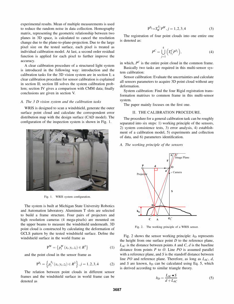
WRIS is designed to scan a windshield, generate the outer

surface point cloud and calculate the correspondent error

distribution map with the design surface (CAD model). The

configuration of the inspection system is shown in Fig. 1.

Fig. 1. WRIS system configuration.

The system is built at Michigan State University Robotics

and Automation laboratory. Aluminum T slots are selected

to build a frame structure. Four pairs of projectors and

high resolution cameras (4 mega-pixels) are mounted on

the upper beams to measure the windshield underneath. 3D

point cloud is constructed by calculating the deformation of

GCLS pattern by the tested windshield surface. Define the

windshield surface in the world frame as

PW ={

pWi (xi,yi,zi) ∈ R3

}

(1)

and the point cloud in the sensor frame as

PSj ={

pS j

i (xi,yi,zi) ∈ R3}

, j = 1,2,3,4 (2)

The relation between point clouds in different sensor

frames and the windshield surface in world frame can be

denoted as

PSj=TS j

W PW , j = 1,2,3,4 (3)

The registration of four point clouds into one entire one

is denoted as:

PC =4

⋃

j=1

(

TCS j

PS j

)

, (4)

in which, PC is the entire point cloud in the common frame.

Basically two tasks are required in this multi-sensor sys-

tem calibration:

Sensor calibration: Evaluate the uncertainties and calculate

all sensors parameters to acquire 3D point cloud without any

deformation.

System calibration: Find the four Rigid registration trans-

formation matrixes to common frame in this multi-sensor

system.

The paper mainly focuses on the first one.

II. THE CALIBRATION PROCEDURE.

The procedure for a general calibration task can be roughly

separated into six steps: 1) working principle of the sensors,

2) system consistence tests, 3) error analysis, 4) establish-

ment of a calibration model, 5) experiments and collection

of data, and 6) parameters identification.

A. The working principle of the sensors

AC

d

hD

D

S

O

c

Oc’

C’

F

Image Plane

Camera

P

A’

Projector

Fig. 2. The working principle of a WRIS sensor.

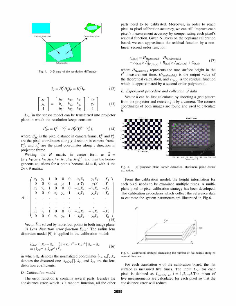
Fig. 2 shows the sensor working principle: hD represents

the height from one surface point D to the reference plane,

LAC is the distance between points A and C, d is the baseline

distance from points P to O. Line PO is assumed parallel

with a reference plane, and S is the standoff distance between

line PO and reference plane. Therefore, as long as LAC, d,

and S are known, hD can be calculated using Eq. 5, which

is derived according to similar triangle theory.

hD =LAC • S

d + LAC

(5)

3687

B. System consistence tests

System consistence performance is an old concept in

robotics area, which evaluates the repeatability of a robot

arm. However, in the machine vision area, few 3D vision

calibration papers discussed it. This is because the random

image noise is low in the traditional inspection range, 10,000

- 50,000 mm2. Large range detection is only used for

navigation purpose, which requires low accuracy.

Current system field of view is about 2,400,000 mm2

with the inspection purpose. With almost 10 times large

standoff distance, the random light intensity noise from

the environment cannot be ignored anymore. The sub-pixel

location for same surface point has a certain level variation.1) Consistence simulation: From Eq. 5, once the input

LAC has a certain magnitude of uncertainties, the height error

will be:

h =

∣

∣

∣

∣

∣

S

1 + dLACRes

−S

1 + d(LAC±LAC)Res

∣

∣

∣

∣

∣

, (6)

where Res represents the resolution converting the unit from

pixel into millimeter. The system is assumed to have 0.1,

0.2, 0.3, and 0.5 pixel error respectively, the errors in height

are shown in the Fig. 3. S is approximately 1500 mm. d is

around 500 mm, and Res equals 0.55 mm/pixel, the average

input of LAC is around 100 pixels in the real case.

Fig. 3. Error analysis results, when the system has 0.1, 0.2, 0.3 and 0.5pixels’ error, the error amount in height.

2) Consistence experimental results: A given windshield

is placed under the WRIS system and measured 10 times.

The standard deviation is used to evaluate the consistence

performance of the system.

From Eq. 5, every camera pixel’s height map hn(i, j),n =1,2, ...,10 is calculated, where i and j stand for the row and

column location of a pixel.

The mean of the height map of each pixel is calculated by

h̄(i, j) = M(h(i, j)) =1

n

k=n

∑k=1

(hn(i, j)) (7)

The standard deviation of each point is

Std(i, j) =

√

1

n

(

h(i, j)− h̄(i, j)

)2(8)

TABLE I

THE STANDARD DEVIATION RESULTS FOR ALL SENSORS

Sensor one Sensor two Sensor three Sensor four

0.17 mm 0.08 mm 0.08 mm 0.13 mm

The standard deviation of a point cloud can be calculated

by

Stds =1

ni • n j

(∑i

∑j

Std(i, j)),(i = 1...,ni, j = 1,...nj), (9)

where ni and n j are the row and column numbers of the

camera resolution, in this application they are 2002 and 2044.

Consistence test results for all sensors are listed in Tab. I.

Comparing the simulation results with the experimental

results in Tab. 1, there is around 0.1 pixel uncertainty noise

in the input LAC. The height map standard deviation is around

0.13 mm in average.

C. Error analysis

Random image noise from environment is amplified as the

sensing system is designed bigger, and consistence of the

system cannot be perfect. Implementation errors also make

differences between the actual case and the theoretic model.

Cameras and projectors cannot be perfectly perpendicular to

the ground in practice, which costs the resolution change.

Different pixels in LAC do not represent same length.

1) Consistence error Econsistence: Consistence analysis can

be viewed as the starting point of the calibration job. Calibra-

tion results will never exceed the consistence performance.

The mean of multi-measurements method is used to reduce

this random error in data collection.

2) Mis-alignment error from both a projector and a

camera Emis−align: From the working principle of the sys-

tem, each pixel’s height map h(i, j) is calculated from input

LAC (i, j) • Res(i, j). If the flat reference plane is perfect

parallel to the image plane, image pixel size on the reference

will be constant. However, implementation always has a

certain angle of mis-alignment.

In Fig. 4, the projector is designed to shoot a square image.

Due to the mis-alignment error, the square pattern is changed

by the homography matrix into a quadrangle. The shape

will warp again when the camera captures the image of the

pattern.

Pr = HrpIP (10)

IC = HCr Pr, (11)

in which, IP is the projector image coordinate, and IC is

the camera image coordinate. Pr = (xr,yr,1)′ is the world

coordinate on the reference board, assuming z = 0 on the

reference board. From Eq. 10 and Eq. 11, Homography

matrix between camera image plane and projector image

plane is shown as:

3688

Projector image plane Camera image plane

Reference plane

Fig. 4. 3-D case of the resolution difference.

IC = HCr Hr

pIP = HCP IP (12)

xC

yC

1

=

h11 h12 h13

h21 h22 h23

h31 h32 h33

xP

yP

1

(13)

LAC in the sensor model can be transferred into projector

plane in which the resolution keeps constant:

LCAC = YC

C −YCA = HC

P (Y PC −YP

A ), (14)

where, LCAC is the pixel distance in camera frame, YC

C and YCA

are the pixel coordinates along y direction in camera frame.

Y PC , and Y P

A are the pixel coordinates along y direction in

projector frame.

Writing the H matrix in vector form as ~h =(h11,h12,h13,h21,h22,h23,h31,h32,h33)

T, and then the homo-

geneous equations for n points become Ah = 0, with A the

2n×9 matrix:

A =

x1 y1 1 0 0 0 −x1X1 −y1X1 −X1

0 0 0 x1 y1 1 −x1Y1 −y1Y −Y1

x2 y2 1 0 0 0 −x2X2 −y2X2 −X2

0 0 0 x2 y2 1 −x2Y2 −y2Y2 −Y2

. . . . . . . . .

. . . . . . . . .

. . . . . . . . .xn yn 1 0 0 0 −xnXn −ynXn −Xn

0 0 0 xn yn 1 −xnYn −ynYn −Yn

(15)

Vector~h is solved by more four points in both image plane.

3) Lens distortion error function Edist : The radius lens

distortion model [9] is applied in the calibration model:

Edist = Xd −Xn =(

1 + kc1r2 + kc2r4)

Xn −Xn

=(

kc1r2 + kc2r4)

Xn(16)

in which Xn denotes the normalized coordinates [xn,yn]′, Xd

denotes the distorted one [xd ,yd ]′]. kc1 and kc1 are the lens

distortion coefficients.

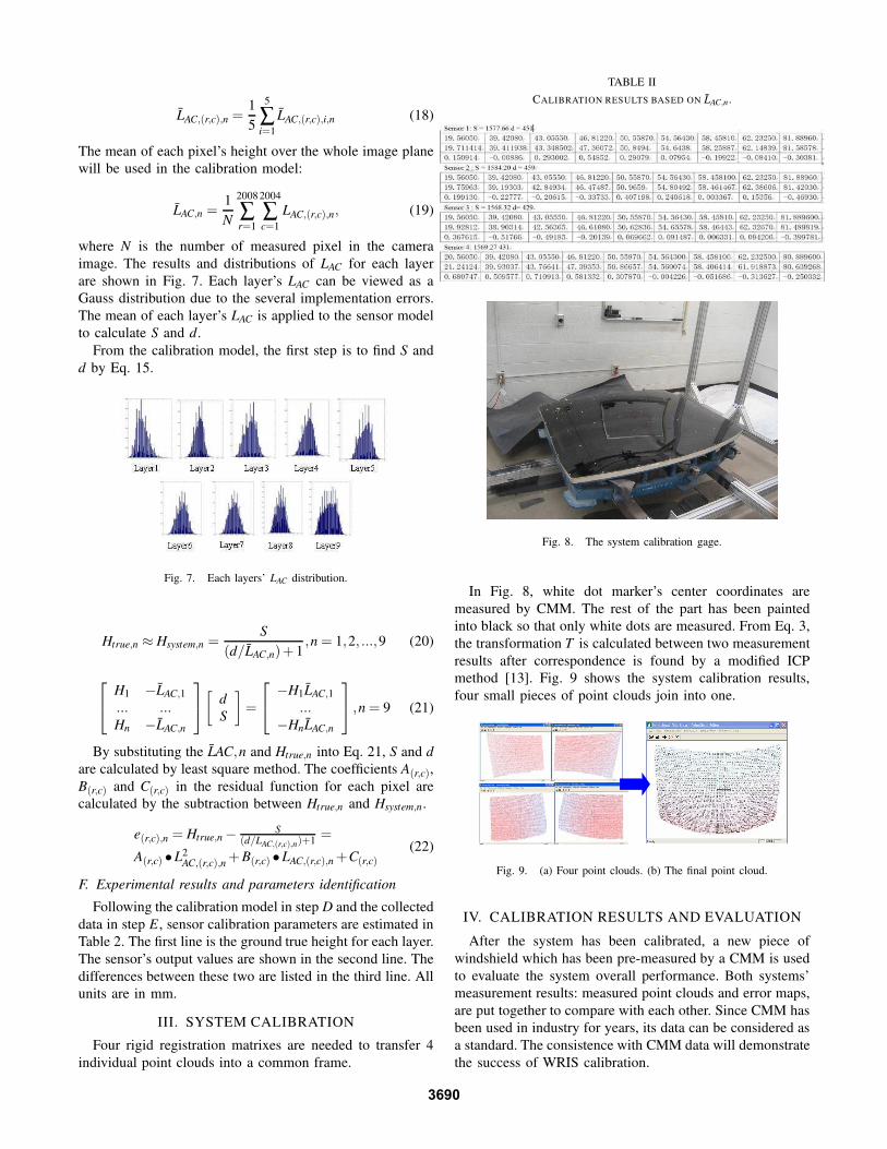
D. Calibration model

The error function E contains several parts. Besides the

consistence error, which is a random function, all the other

parts need to be calibrated. Moreover, in order to reach

pixel-to-pixel calibration accuracy, we can still improve each

pixel’s measurement accuracy by compensating each pixel’s

residual function. Given N layers on the coplanar calibration

board, we can approximate the residual function by a non-

linear second order function:

ei,(r,c) = HMeasured,i −HIdealmodel,i

= A(r,c)×L2AC,i,(r,c) + B(r,c)×LAC,i,(r,c) +C(r,c),

(17)

where HMeasured,i represents the true surface height in the

ith measurement time. HIdealmodel,i is the output value of

the theoretical calculation, and ei,(r,c) is the residual function

which is approximated by a second order polynomial.

E. Experiment procedure and collection of data

Vector~h can be first calculated by shooting a grid pattern

from the projector and receiving it by a camera. The corners

coordinates of both images are found and used to calculate~h.

Fig. 5. (a) projector plane corner extraction, (b)camera plane cornerextraction.

From the calibration model, the height information for

each pixel needs to be examined multiple times. A multi-

plane pixel-to-pixel calibration strategy has been developed.

The calibration procedures which collect the reference data

to estimate the system parameters are illustrated in Fig.6.

Fig. 6. Calibration strategy: Increasing the number of flat boards along itsnormal direction.

For each translation n of the calibration board, the flat

surface is measured five times. The input LAC for each

pixel is denoted as LAC,(r,c),i,n, i = 1,2, ..,5.The mean of

five measurements are calculated for each pixel so that the

consistence error will reduce:

3689

L̄AC,(r,c),n =1

5

5

∑i=1

L̄AC,(r,c),i,n (18)

The mean of each pixel’s height over the whole image plane

will be used in the calibration model:

L̄AC,n =1

N

2008

∑r=1

2004

∑c=1

LAC,(r,c),n, (19)

where N is the number of measured pixel in the camera

image. The results and distributions of LAC for each layer

are shown in Fig. 7. Each layer’s LAC can be viewed as a

Gauss distribution due to the several implementation errors.

The mean of each layer’s LAC is applied to the sensor model

to calculate S and d.

From the calibration model, the first step is to find S and

d by Eq. 15.

Fig. 7. Each layers’ LAC distribution.

Htrue,n ≈ Hsystem,n =S

(d/L̄AC,n)+ 1,n = 1,2, ...,9 (20)

H1 −L̄AC,1

... ...Hn −L̄AC,n

[

d

S

]

=

−H1L̄AC,1

...−HnL̄AC,n

,n = 9 (21)

By substituting the L̄AC,n and Htrue,n into Eq. 21, S and d

are calculated by least square method. The coefficients A(r,c),

B(r,c) and C(r,c) in the residual function for each pixel are

calculated by the subtraction between Htrue,n and Hsystem,n.

e(r,c),n = Htrue,n −S

(d/LAC,(r,c),n)+1=

A(r,c) •L2AC,(r,c),n + B(r,c) •LAC,(r,c),n +C(r,c)

(22)

F. Experimental results and parameters identification

Following the calibration model in step D and the collected

data in step E , sensor calibration parameters are estimated in

Table 2. The first line is the ground true height for each layer.

The sensor’s output values are shown in the second line. The

differences between these two are listed in the third line. All

units are in mm.

III. SYSTEM CALIBRATION

Four rigid registration matrixes are needed to transfer 4

individual point clouds into a common frame.

TABLE II

CALIBRATION RESULTS BASED ON L̄AC,n .

Fig. 8. The system calibration gage.

In Fig. 8, white dot marker’s center coordinates are

measured by CMM. The rest of the part has been painted

into black so that only white dots are measured. From Eq. 3,

the transformation T is calculated between two measurement

results after correspondence is found by a modified ICP

method [13]. Fig. 9 shows the system calibration results,

four small pieces of point clouds join into one.

Fig. 9. (a) Four point clouds. (b) The final point cloud.

IV. CALIBRATION RESULTS AND EVALUATION

After the system has been calibrated, a new piece of

windshield which has been pre-measured by a CMM is used

to evaluate the system overall performance. Both systems’

measurement results: measured point clouds and error maps,

are put together to compare with each other. Since CMM has

been used in industry for years, its data can be considered as

a standard. The consistence with CMM data will demonstrate

the success of WRIS calibration.

3690

The CMM measurement point cloud is denoted as{

PCMM

(

xCi ,yC

i ,zCi

)

∈ R3}

, and the WRIS result is denoted

as{

PWRIS

(

xWi ,yW

i ,zWi

)

∈ R3}

, The mean error is used to

find the difference between both point clouds:

Mean =1

N

N

∑i=1

[

(

xWi − xC

i

)2+

(

yWi − yC

i

)2+

(

zWi − zC

i

)2]1/2

(23)

The difference between CMM data and WRIS data is

about 0.15 mm, which is around 0.14 pixel in backprojected

images into cameras. Compared with the results [11], their

overall backprojected pixel errors are 0.02 pixel in camera

and 0.29 pixel in projector. Since in our sensor model

the projector’s intrinsic and extrinsic parameters do not

participate in the calculation, 3D points in world are directly

correspondence with projector pixels. Backprojected error in

projector can be viewed as 0 pixel.

Fig. 10 and Fig. 11 illustrate that both CMM data and the

WRIS point cloud has the similar error distribution shape

and the same error color magnitudes.

Fig. 10. The CMM error map.

Fig. 11. The WRIS error map.

V. CONCLUSION

A clear calibration procedure of a structure light vision

system has been implemented when the 3D sensor has a

relatively large field of inspection. Calibration tasks can be

separated into two categories: sensor calibration and system

calibration. The main effort is concentrated on the sensor

calibration. A detailed calibration model and error analysis

are developed due to the increasing number of uncertainties.

Pixel-to-pixel calibration strategy is applied to reach the ac-

curacy requirement. System calibration uses Iterative Closed

Point (ICP) [13] method to solve the correspondence problem

and calculates the rigid transformation matrix between each

sensor to world frame. The calibrated WRIS is able to sample

a given piece of windshield and generate a point cloud of

more than 30000 points within 20 seconds. Experimental

results show the system calibration results are comparable

with a CMM system. The calibration method is feasible for

the task.

REFERENCES

[1] Pages J, Salvi J, Garcia R, and Matabosch C. Overview of coded lightprojection techniques for qutomatics 3 D profiling, In Proceedings

of IEEE international conference on robotics and automation, Taipei,Taiwan, 2003, pp. 133-138.

[2] Kurada, S., and Bradley. C., A review of machine vision sensors fortool condition monitoring, Comput. Ind., 34, No. 1, pp. 55-72, 1997.

[3] Q. Shi, N. Xi, and H. Chen, ”Integrated process for measurement offree-form automotive part surface using a digital area sensor,” in IEEEInternational Conference on Robotics and Automation,Alera, Canada,2005, pp.1526- 1531.

[4] M. Trobina, ”Error Model of a Coded-Light Range Sensor,” BIWI-TR-164, Sept. 21, 1995.

[5] Z. Yang, and Y.F. Wang, Error Analysis of 3 D Shape Constructionfrom Structured Lighting, Pattern Recognition, Vol. 29, No. 2, pp.189-206, 1996.

[6] G. Sansoni, M. Carocci, and T. Rodella, Calibration and PerformanceEvaluation of a 3-D Imaging Sensor Based on the Projection of Struc-tured Light, IEEE Transactions on Instrumentation and Measurement,Vol. 49, No. 3, pp. 628-536, 2000.

[7] P. Chen and D. Suter, ”Homography estimation and heteroscedasticnoise-a first order perturbation analysis,” Monash University, Tec. Rep.MECSE-32, 2005.

[8] R. Hartley and A. Zisserman, Multiple View Geometry in ComputerVision, Cambridge U.Press, 2003, Chap. 5, pp.132 - 150.

[9] R. Tsai, A Versatile Camera Calibration Technique for High-Accuracy3D Machine Vision Metrology Using Off-the-Shelf TV Cameras andLenses, IEEE Journal of Robotics and Automation, Vol. Ra-3, No. 4,1987.

[10] Q. Shi, N. Xi, H. Chen, and Y. Chen, ”Calibration of RoboticArea Sensing System for Dimensional Measurement of AutomotivePart Surfaces,” in International Conference on Intelligent Robots andSystems, Alberta, Canada, Aug. 2005, pp. 1526-1531.

[11] B. Zhang, and Y. Li, Dynamic calibration of the relative pose anderror analysis in a structured light system, J. Opt. Soc., Vol. 25, No.3.pp 612 -622. March. 2008.

[12] C. Zhang, N. Xi, Q. Shi, ”Object-Orientated Registration Methodfor Surface Inspection of Automotive Windshields,” in International

Conference on Intelligent Robots and Systems, Nice, France, Sep.2008, pp. 3553-3558.

[13] P. J. Besl and N. D. Mckay, A Method for Registration of 3-D Shapes,IEEE Transactions on Pattern Analysis and Machine Intelligence, vol.14. no.2, 1992, pp 239-255.

[14] J. Mosnier, F. Berry and O. A. Aider, ”A New Method for Projec-tor Calibration Based on Visual Servoing,” in IAPR Conference on

Machine Vision Applications, Yokohama, Japan, May 20-22, 2009, pp25-29.

[15] J. Drarei, and S. Roy, ”Projector Calibration Using a MarkerlessPlane,” in Proceedings of the Interenational Conference on Computer

Vision Theory and Applications, Lisbon, Portugal, Feb 2009, volume2, pp 377 -382.

3691