MULTI-SCALE MODELING AND SIMULATION OF SEMI-FLEXIBLE FILAMENTS

By

GAURAV MISRA

A DISSERTATION PRESENTED TO THE GRADUATE SCHOOLOF THE UNIVERSITY OF FLORIDA IN PARTIAL FULFILLMENT

OF THE REQUIREMENTS FOR THE DEGREE OFDOCTOR OF PHILOSOPHY

UNIVERSITY OF FLORIDA

2010

c© 2010 Gaurav Misra

2

I dedicate this to my family and God.

3

ACKNOWLEDGMENTS

This dissertation would never have come to fruition without the kind support of

many individuals, and it is with pleasure that I proffer my sincere gratitude towards them

all. I am immeasurably indebted to my advisors, Prof. Tony Ladd and Prof. Richard

Dickinson, for their exhaustless patience, invaluable guidance, and the unwavering

support they have provided me through difficult and easy times alike. I am grateful to

Prof. Tanmay Lele for the mentoring and career counseling he has granted me; it has

been a pleasure and a learning experience to work with him. I thank Prof. Daniel Purich

for the active interest and clarity with which he nurtures students’ understanding of

science, in general, and structural biochemistry, in particular. Financial support for this

work has come from the National Science Foundation (grant no. CTS-0505929).

Prof. Jason Butler provided me with additional computational resources, without

which this work could not have been completed in time. I thank Prof. Yiider Tseng and

Prof. Loc Vu-Quoc for their critical comments on my work and writing skills. Dr. Berk

Usta, a former student of Dr. Ladd and Dr. Butler, has provided me with insightful career

advice and I am thankful for his counseling and friendship. I acknowledge my labmates,

Dr. Ulf Schiller, Rahul Kekre, and Virat Upadhyay for stimulating discussions. Robert

Russell and Jun Wu, Dr. Lele’s graduate students, have performed all the experiments

for my last modeling project.

I would like to thank Shirley Kelly and Deborah Sandoval (Debbie) from the

departmental staff for their kind help and friendship throughout these years. I am

grateful to my parents who capacitated me in every way to pursue the arduous but

rewarding goal of earning the highest academic degree. Last but not the least, I thank

my loving wife, Neha, whose thoughtful and diligent care saw me through all my ordeals.

4

TABLE OF CONTENTS

page

ACKNOWLEDGMENTS . . . . . . . . . . . . . . . . . . . . . . . . . . . . . . . . . . 4

LIST OF TABLES . . . . . . . . . . . . . . . . . . . . . . . . . . . . . . . . . . . . . . 7

LIST OF FIGURES . . . . . . . . . . . . . . . . . . . . . . . . . . . . . . . . . . . . . 8

ABSTRACT . . . . . . . . . . . . . . . . . . . . . . . . . . . . . . . . . . . . . . . . . 10

CHAPTER

1 INTRODUCTION AND BACKGROUND . . . . . . . . . . . . . . . . . . . . . . 11

2 ALGORITHM FOR INTEGRATING THE E.O.M. OF ELASTIC RODS . . . . . . 13

2.1 Introduction . . . . . . . . . . . . . . . . . . . . . . . . . . . . . . . . . . . 132.2 Elastic Filament Models . . . . . . . . . . . . . . . . . . . . . . . . . . . . 152.3 Discrete Equations of Motion . . . . . . . . . . . . . . . . . . . . . . . . . 212.4 Hamiltonian Formulation . . . . . . . . . . . . . . . . . . . . . . . . . . . . 25

2.4.1 Hamiltonian for an Elastic Filament . . . . . . . . . . . . . . . . . . 262.4.2 Discretized Hamiltonian . . . . . . . . . . . . . . . . . . . . . . . . 282.4.3 Operator Splitting . . . . . . . . . . . . . . . . . . . . . . . . . . . . 30

2.5 Numerical Examples . . . . . . . . . . . . . . . . . . . . . . . . . . . . . . 322.5.1 A Filament Bent into a Circle . . . . . . . . . . . . . . . . . . . . . 322.5.2 A Filament Bent into a Helix . . . . . . . . . . . . . . . . . . . . . . 37

2.6 Conclusions . . . . . . . . . . . . . . . . . . . . . . . . . . . . . . . . . . . 39

3 MECHANICS OF VORTICELLA . . . . . . . . . . . . . . . . . . . . . . . . . . 41

3.1 Introduction . . . . . . . . . . . . . . . . . . . . . . . . . . . . . . . . . . . 413.2 Model and Simulations . . . . . . . . . . . . . . . . . . . . . . . . . . . . . 43

3.2.1 Mechanical Model . . . . . . . . . . . . . . . . . . . . . . . . . . . 433.2.2 Chemical Model . . . . . . . . . . . . . . . . . . . . . . . . . . . . . 463.2.3 Geometric Constraints . . . . . . . . . . . . . . . . . . . . . . . . . 473.2.4 Parameter Estimation . . . . . . . . . . . . . . . . . . . . . . . . . 49

3.2.4.1 Geometric and mechanical parameters . . . . . . . . . . 493.2.4.2 Chemical parameters . . . . . . . . . . . . . . . . . . . . 51

3.3 Results . . . . . . . . . . . . . . . . . . . . . . . . . . . . . . . . . . . . . 533.3.1 Fast Binding . . . . . . . . . . . . . . . . . . . . . . . . . . . . . . . 533.3.2 Delayed Binding . . . . . . . . . . . . . . . . . . . . . . . . . . . . 553.3.3 Recovery . . . . . . . . . . . . . . . . . . . . . . . . . . . . . . . . 58

3.4 Discussion . . . . . . . . . . . . . . . . . . . . . . . . . . . . . . . . . . . 59

5

4 CYTO-MECHANICS OF MICROTUBULAR BUCKLING AND CENTERINGOF CENTROSOME . . . . . . . . . . . . . . . . . . . . . . . . . . . . . . . . . 63

4.1 Introduction . . . . . . . . . . . . . . . . . . . . . . . . . . . . . . . . . . . 634.2 Modeling . . . . . . . . . . . . . . . . . . . . . . . . . . . . . . . . . . . . 65

4.2.1 MT Model . . . . . . . . . . . . . . . . . . . . . . . . . . . . . . . . 654.2.2 Dynein Model . . . . . . . . . . . . . . . . . . . . . . . . . . . . . . 664.2.3 Microtubular Dynamic Instability Model . . . . . . . . . . . . . . . . 674.2.4 Cell Periphery Model . . . . . . . . . . . . . . . . . . . . . . . . . . 694.2.5 Multiscale Model . . . . . . . . . . . . . . . . . . . . . . . . . . . . 714.2.6 Parameters . . . . . . . . . . . . . . . . . . . . . . . . . . . . . . . 72

4.3 Results . . . . . . . . . . . . . . . . . . . . . . . . . . . . . . . . . . . . . 744.3.1 Buckling of Polymerizing MTs Against Cell Membrane . . . . . . . 744.3.2 Buckling of a Cut MT . . . . . . . . . . . . . . . . . . . . . . . . . . 764.3.3 Anterograde Movement of Bends . . . . . . . . . . . . . . . . . . . 764.3.4 Centrosome Centering In-Vivo . . . . . . . . . . . . . . . . . . . . 774.3.5 In-Vitro Centering of Centrosome by Polymerization Forces . . . . 81

4.4 Discussion . . . . . . . . . . . . . . . . . . . . . . . . . . . . . . . . . . . 84

5 SUMMARY . . . . . . . . . . . . . . . . . . . . . . . . . . . . . . . . . . . . . . 87

APPENDIX

A PROPERTIES OF QUATERNIONS . . . . . . . . . . . . . . . . . . . . . . . . . 89

B CICR BASED SIGNAL SPEED . . . . . . . . . . . . . . . . . . . . . . . . . . . 93

REFERENCES . . . . . . . . . . . . . . . . . . . . . . . . . . . . . . . . . . . . . . . 95

BIOGRAPHICAL SKETCH . . . . . . . . . . . . . . . . . . . . . . . . . . . . . . . . 106

6

LIST OF TABLES

Table page

2-1 Properties of quaternions (Appendix A) . . . . . . . . . . . . . . . . . . . . . . 22

3-1 Geometric parameters . . . . . . . . . . . . . . . . . . . . . . . . . . . . . . . . 52

3-2 Mechanical parameters . . . . . . . . . . . . . . . . . . . . . . . . . . . . . . . 52

3-3 Chemical parameters . . . . . . . . . . . . . . . . . . . . . . . . . . . . . . . . 52

4-1 Microtubule parameters . . . . . . . . . . . . . . . . . . . . . . . . . . . . . . . 71

4-2 Dynein parameters . . . . . . . . . . . . . . . . . . . . . . . . . . . . . . . . . . 72

4-3 Miscellaneous parameters . . . . . . . . . . . . . . . . . . . . . . . . . . . . . . 72

7

LIST OF FIGURES

Figure page

2-1 Schematic of the elastic rod model . . . . . . . . . . . . . . . . . . . . . . . . . 15

2-2 Filament shapes at different times . . . . . . . . . . . . . . . . . . . . . . . . . 33

2-3 Energy conservation plots . . . . . . . . . . . . . . . . . . . . . . . . . . . . . . 34

2-4 Energy conservation comparison of OSDH and MPDH . . . . . . . . . . . . . . 36

2-5 Shapes of a helically bent rod . . . . . . . . . . . . . . . . . . . . . . . . . . . . 38

2-6 Thermalization of a helically bent rod . . . . . . . . . . . . . . . . . . . . . . . . 39

3-1 Images of V. Convallaria and the model . . . . . . . . . . . . . . . . . . . . . . 42

3-2 Schematic of the stalk-spasmoneme model . . . . . . . . . . . . . . . . . . . . 45

3-3 Time lapse images of the initial phase of contraction driven by instantaneousbinding . . . . . . . . . . . . . . . . . . . . . . . . . . . . . . . . . . . . . . . . 54

3-4 Simulation results for contraction driven by instantaneous binding. . . . . . . . 55

3-5 Results for Young’s modulus= 1 kPa and different values of rate constant. . . . 56

3-6 Images of contraction with Young’s modulus = 1 kPa and rate constant = 5 ×105 M−1s−1. . . . . . . . . . . . . . . . . . . . . . . . . . . . . . . . . . . . . . . 57

3-7 Velocity profiles for different viscosities. . . . . . . . . . . . . . . . . . . . . . . 57

3-8 Recovery simulations . . . . . . . . . . . . . . . . . . . . . . . . . . . . . . . . 58

4-1 Images of centrosome location in patterned cells. . . . . . . . . . . . . . . . . . 64

4-2 Schematic of the dynein model. . . . . . . . . . . . . . . . . . . . . . . . . . . . 65

4-3 Microtubular length distribution. . . . . . . . . . . . . . . . . . . . . . . . . . . . 69

4-4 Angle of incidence of MT on periphery. . . . . . . . . . . . . . . . . . . . . . . . 70

4-5 MT cut in dynein inhibited cells. . . . . . . . . . . . . . . . . . . . . . . . . . . . 73

4-6 Experimental observation of polymerizing and buckling MTs. . . . . . . . . . . 74

4-7 Simulations of MTs polymerizing against a soft barrier. . . . . . . . . . . . . . . 75

4-8 Single MT cutting experiment. . . . . . . . . . . . . . . . . . . . . . . . . . . . . 76

4-9 Simulation of cutting MTs. . . . . . . . . . . . . . . . . . . . . . . . . . . . . . . 77

4-10 Anterograde propogation of bends in MTs. . . . . . . . . . . . . . . . . . . . . . 78

8

4-11 Autocorrelation of centrosome position in control cells. . . . . . . . . . . . . . . 78

4-12 Simulations of centrosome positioning without dynein motors. . . . . . . . . . . 79

4-13 Plot of centrosome position without dynein motors. . . . . . . . . . . . . . . . . 80

4-14 Simulations of centrosome positioning with dynein motors. . . . . . . . . . . . . 80

4-15 Plot of centrosome position with dynein motors. . . . . . . . . . . . . . . . . . . 81

4-16 Simulation of in-vitro pushing of centrosome by short MTs. . . . . . . . . . . . 82

4-17 Simulation of in-vitro pushing of centrosome by long MTs. . . . . . . . . . . . . 83

4-18 Plots of centrosome position in small glass chamber. . . . . . . . . . . . . . . . 83

4-19 Plots of centrosome position in small glass chamber. . . . . . . . . . . . . . . . 84

9

Abstract of Dissertation Presented to the Graduate Schoolof the University of Florida in Partial Fulfillment of theRequirements for the Degree of Doctor of Philosophy

MULTI-SCALE MODELING AND SIMULATION OF SEMI-FLEXIBLE FILAMENTS

By

Gaurav Misra

December 2010

Chair: Anthony J.C. LaddCochair: Richard B. DickinsonMajor: Chemical Engineering

Elastic rods are a ubiquitous model of semi-flexible biopolymers such as DNA, actin,

and microtubules. We developed a stable, energy-conserving and constraint-free

algorithm for integrating the equations of motion of elastic rods. Tests show that

our algorithm is much more stable and faster than the standard formulations. This

model is employed to understand the dynamics of biophysical systems which have

filamentous structures as the key elements. For example, we have developed a

mechano-chemical model of Vorticella, one of the fastest organisms on the planet

(relative to its size). It moves by coiling a slender stalk-like tether which attaches it

to a substrate. Simulations quantitatively capture the experimental observations and

offer insights into the mechanics and chemistry of the organism’s quick movement. We

have also modeled the cyto-mechanics underlying the positioning of the centrosome

of a cell. A model for the microtubular network has been developed and coupled with

a model for force generation by dynein motors. Simulations show that even buckled

microtubules can be under tension through most of their length. We demonstrate the

consequences of two contradictory models of centrosome centering – one assuming

that the microtubules in a cell are under compression and the other assuming that they

are under tension.

10

CHAPTER 1INTRODUCTION AND BACKGROUND

In the latter half of the 20th century, our understanding of biological systems was

revolutionized by the advent of Biochemistry, which discovered the molecular principles

underlying several biological processes previously considered intractable. Biophysics

is now playing a similar role by striving to integrate the mechanical and chemical

processes in living organisms in order to provide a complete picture of living systems. A

cell is no longer viewed as a compartmentalized bag of chemicals but a highly integrated

multi-scale physio-chemical system, which must be studied as a whole. Physical forces

in a cell were considered as the outcome of the underlying chemical reactions, without

any role to play in the decision making processes. However, physical forces are being

discovered to be intimately linked with the regulation of several biological functions [1].

This work seeks to add to our understanding of physics in biological system and its

integration with some of the chemical processes.

Several biological phenomena like endo and exo-cytosis, cell division and migration,

have significant mechanical components to them. The mechanical components of a cell

include membranous structures and filaments. Although largely consisting of water, the

cellular environment exhibits material properties much different from that of pure water

due to the intricate microstructure provided by the filaments and membranes. The key

to understanding the dynamics of cells hinges on understanding the dynamics of the

individual mechanical components and their integration with each other and with the

chemical processes in the cell.

The mechanical components of cells can be classified as soft matter, which is the

class of matter lying between solids and liquids. Most of the predominant dynamics of

soft matter happen on the thermal scale. Cell membranes, organelle membranes, actin

filaments, microtubules (MTs), intermediate filaments (IFs), and cilia are examples of

biologically relevant soft matter. Significant emphasis is being laid on understanding

11

the small and large scale behavior of these materials. Molecular simulations shed

light on the small-scale and short-time dynamics of these materials [2, 3]. Since the

biologically relevant time scales (minutes to hours) are currently beyond the reach of

MD, coarse-grain models utilizing constitutive laws, like elasticity, are being used to

study the long-time dynamics of these systems [4–8]. The hydrodynamic interactions

of soft matter components is another exciting field of research which incorporates the

ever-present medium into the dynamics of membranes and filaments [9, 10].

Filamentous structures play an important role in locomotion, transport of material,

sensation and structural integrity. The coordinated motion of cilia is responsible for

mucociliary clearance (transport of mucus) in the respiratory tract, for transport of

ovum in the fallopian tubes, and for locomotion in many unicellular organisms [11, 12].

The mechanics of filamentous structures in auditory hair cells plays a critical role in

sound reception and amplification [13, 14]. The acrosomal process involves coiling and

uncoiling of bundled actin filaments, the mechanics of which is not yet understood.

From a cellular rheology perspective, the visco-elasticity of cells is largely attributed

to the microstructure [15, 16] derived from the fluid filled network of F-actin, MTs, and

IFs, which constitute the cytoskeleton of a cell. Actin filaments are also responsible

for motility in some systems [17–20]. Microtubular mechanics plays a critical role in

chromosomal separation and cell division [21–25].

This work focuses on modeling the dynamics of elastic rods for applications to

biological systems. The second chapter details a new algorithm for solving the full

equations of motion of an elastic rod in a numerically stable and accurate manner. An

application of the model is described in the third chapter where we couple the rod model

with a chemical model in order to understand the mechanics of Vorticella Convallaria,

which is interesting due to its extremely fast movement. The fourth chapter addresses

the mechanics of centrosome centering using a multi-scale model of the microtubular

aster growing from the centrosome.

12

CHAPTER 2ALGORITHM FOR INTEGRATING THE E.O.M. OF ELASTIC RODS

2.1 Introduction

Elastic rods are a ubiquitous model of semi-flexible biopolymers such as DNA

[7, 26–32], actin [33–36], and microtubules [23]. They can also be found in a diverse

range of applications including catheter navigation [37], undersea cables [38], and

organismal biology [39]. In biophysics, the worm-like chain (WLC) model [27, 40]

underpins many theoretical [36, 41–47] and numerical [48–51] studies of semiflexible

polymers. The WLC model is a linearization of the classical Kirchhoff rod model [52, 53],

which is itself a limiting case where the product of the local curvature and filament

thickness is everywhere small [54]. In this limit the shear and extensional strains are

negligible but the constraint forces generated by them are not. In this work we consider

a generalization of the Kirchhoff model [5, 55], where the shear and extensional strains

are explicitly accounted for by an elastic constitutive model, eliminating the need for

constraint forces at the cost of an additional time scale; such models are frequently

referred to as “geometrically exact” in the finite-element literature [5, 55].

The dynamics of Kirchhoff or geometrically exact (GE) filaments is typically

determined by finite-element or finite-difference approximations, but the stiffness of

the numerical system has proved to be a difficult and long-standing problem [56–58].

Significant progress has been made by developing implicit methods that exactly satisfy

the constraints of momentum and energy conservation [55, 59], yet even here artificial

dissipation is often needed for long-term stability [60]. On the other hand, in discrete

dynamical systems it is known that symplectic integration methods give superior

long-term stability in comparison with either high-order explicit or implicit integration

methods [61]; the most common symplectic integrator is the Verlet algorithm [62].

Symplectic integrators generate a sequence of canonical transformations, which do not

exactly conserve energy but do preserve the density of points in the phase space, along

13

with the Poincare invariants. In recent years symplectic integrators have been developed

for both linear and angular motions [61, 63, 64]. The objective of this project is to explore

a symplectic integration method for geometrically exact filament models. This requires

both a Hamiltonian approximation to the partial differential equations describing the

filament dynamics, and a symplectic integrator.

The proposed algorithm is based on a discretization of the Hamiltonian line integral

of an elastic filament, including shear and extensional degrees of freedom. Since the

nodal forces and torques follow from an exact differentiation of a potential function, the

equations of motion are guaranteed to be Hamiltonian, although the potential function

itself is only an approximation to the continuum limit. This is in contrast to finite-element

methods, where the continuum equations of motion are discretized in space; in this case

the Hamiltonian structure is not preserved, even if the total energy is conserved [55]. In

fact, it can be shown that for any approximate solution it is not possible to maintain both

the symplectic structure and exact energy conservation simultaneously [65].

An outline of the chapter is as follows. In Sec. 2.2 we describe different models

of elastic filaments–GE, Kirchhoff, WLC–and indicate how they are related. Next

(Sec. 2.3), we derive a simple finite-difference approximation of the equations of motion

of a GE filament model, as a basis for comparison with the Hamiltonian formulation

presented in Sec. 2.4. We note that the Hamiltonian approach has only been followed

occasionally [66], and in that case for the Kirchhoff rod model. We will argue (Sec. 2.5)

that the absence of geometric constraints in the GE model offers computational

advantages over the Kirchhoff model when there are excluded volume interactions

between the segments. We replace the usual implicit time integration [55, 66] with an

explicit operator splitting method [63], which eliminates the repeated force evaluations

of an implicit method. The numerical scheme is stable and energy conserving even for

large deformations; we illustrate this by numerical example in Sec. 2.5. Our conclusions

and future outlook are in Sec. 2.6.

14

02d

d30

1d 0

2d

1d

d3

s

s

(b)

(a)

Figure 2-1. An elastic filament in the unstrained (reference) state (a) and afterdeformation (b). In the reference state, the material plane, shown by thesolid ellipse, is aligned with its normal parallel to the tangent to the centerline(dashed line). The local director basis of the reference state, d0

i (s), and thedeformed state, di (s), are also shown. A material point (solid black circle)moves with the translation and rotation of the local coordinate system; in thiscase extension, shear, bend, and twist can all be seen.

2.2 Elastic Filament Models

The classical Kirchhoff theory of elastic rods has been elegantly and concisely

described in the “Theory of Elasticity” by Landau and Lifshitz [53], and the seminal book

by Love [52]. More rigorous derivations of the equations of motion are available in the

literature [54, 67]. Here we summarize the key concepts and establish the notation to be

used later in the chapter. An elastic filament (or thin rod) is described by the coordinates

15

of its centerline r(s) and a set of orthonormal directors d1(s), d2(s), d3(s). The directors

establish the orientation of a cross section or material plane at the location s, where s is

a parametric coordinate defining the position of each point along the centerline. In the

undeformed filament, s is the contour length from the origin. We will choose a body-fixed

coordinate system such that d1 and d2 point along the principal axes of inertia of the

cross section and therefore d3 = d1 × d2 is normal to the material plane; the coordinate

system is illustrated in Fig 2-1. If the rod has a circular cross section then the initial

choice of d1 and d2 contains an arbitrary rotation about d3. In contrast with the Kirchhoff

theory, we will not assume that d3 is constrained to be parallel to the tangent vector ∂sr

(Fig 2-1b).

The key assumption of thin-rod elasticity is that there is no deformation within a

material plane, only translation and rotation of that plane. Deformation of an elastic

filament is then described by two one-dimensional strain fields, �(s) and (s),

describing the rate of change of the centerline position and director vectors along

the filament [5, 55]

�1 = d1 · (∂sr) 1 = d3 · (∂sd2) = −d2 · (∂sd3)

�2 = d2 · (∂sr) 2 = d1 · (∂sd3) = −d3 · (∂sd1)

�3 = d3 · (∂sr) 3 = d2 · (∂sd1) = −d1 · (∂sd2).

(2–1)

A thin segment of the filament can be subjected to six different deformations. �1 and �2

describe transverse motions of a material plane with respect to the normal vector (d3),

which causes shearing of the segment, while �3 describes extension or compression of

the segment. Bending of the segment about its principal axes is described by 1 and

2, and twisting of the segment by 3. Uniform deformation corresponds to constant

values of � and ; for example, in a straight rod � = [0, 0, 1] and = [0, 0, 0]. More

interestingly, a helical rod can be described by a constant bend and twist, � = [0, 0, 1],

= [Rκ2, 0, Pκ2], where R is the radius of the helix, 2πP is the pitch, and the combined

curvature due to bend and twist, κ = (P2 + R2)−1/2. The choice of signs define a

16

right-handed helix, r(s) = [R cos(κs), R sin(κs), Pκs], with basis vectors

d1 = [Pκ sin(κs),−Pκ cos(κs), Rκ]

d2 = [cos(κs), sin(κs), 0]

d3 = [−Rκ sin(κs), Rκ cos(κs), Pκ].

(2–2)

The stresses in the rod are assumed to be linear in the deviations in the strain

fields, ��i = �i − �0i and �i = i −0

i , from the reference (stress free) configuration �0,

0. It is convenient to define the strains in the body-fixed coordinate system, since the

elastic constant matrix is then diagonal. The force F �i and couple F

i on each material

plane are [52, 53]

F �i = C �

i ��i , F i = C

i �i , (2–3)

where the elastic constants for each deformation are, in principle, independent. In

the GE model, the strain energy density U(s) contains contributions from shear and

extension, in addition to the usual bend and twist of the Kirchhoff model,

U = U� + U =12

3∑

i=1

(C �

i ��2i + C

i �2i

). (2–4)

For an isotropic material, the elastic moduli for shear (C �1,2), extension (C �

3 ), bend

(C 1,2), and twist (C

3 ) are given by:

C �1 = GA C

1 = YI1

C �2 = GA C

2 = YI2

C �3 = YA C

3 = GI3,

(2–5)

where G is the shear modulus, Y is Young’s modulus, A is the area of the cross-section

and I1 and I2 are its principle moments of inertia. For rods with a circular cross section,

I3 = I1 + I2, but in the general case there is an additional contribution from the warping of

the cross section [53], so that I3 is then distinct from I1 + I2. The elastic coefficients can

also be determined empirically, without reference to any particular constitutive law.

17

The velocity and angular velocity of the segment are defined in an analogous

fashion to the strain fields in Eq. 2–1,

v1 = d1 · (∂tr) ω1 = d3 · (∂td2) = −d2 · (∂td3)

v2 = d2 · (∂tr) ω2 = d1 · (∂td3) = −d3 · (∂td1)

v3 = d3 · (∂tr) ω3 = d2 · (∂td1) = −d1 · (∂td2).

(2–6)

The kinetic energy density of the filament is then [52, 53]

T = T � + T =12

3∑

i=1

(M�

i v 2i + M

i ω2i

), (2–7)

where the generalized mass densities associated with shear (M�1 , M�

2 ), extension (M�3 ),

bend (M1 , M

2 ) and twist (M3 ), are

M�i = ρA, M

i = ρIi , (2–8)

and ρ is the mass density of the filament.

Equations of motion for the filament can be derived from the balance of linear and

angular momenta in a thin segment bounded by the planes s and s + ds. The rate of

change of the linear momentum of the segment, pds, is

_pds = F�(s + ds)− F�(s), (2–9)

where p =∑3

i=1 M�vi di is the linear momentum density (per unit length). The forces on

the two planes must be differenced in a common coordinate frame, which we take as the

space-fixed frame. The balance of angular momentum in the segment lds involves both

couples and moments of the force,

_lds = F(s + ds)− F(s) + [r(s + ds)− r(s)]× F�(s), (2–10)

18

where l =∑3

i=1 Mi ωi di is the linear angular momentum density. Thus the equations of

motion of a GE filament are

_p = ∂sF�, (2–11)

_l = ∂sF + r′ × F�, (2–12)

where r′ = ∂sr indicates a spatial derivative along the filament. A finite-difference

approximation to these equations is described in Sec. 2.3.

Equations 2–11–2–12 describe the dynamics of the GE rod model [5, 55]. The

difference with the Kirchhoff theory is that, here, the force on a material plane, F �i , is

given by a constitutive equation, Eq. (2–3), based on the deflection and extension of the

local tangent vector relative to the material plane, Eq (2–1). In the Kirchhoff model the

tangent vector is constrained to remain parallel to d3 (unshearable) and of unit length

(inextensible), or in other words ��i = 0 and r′ = d3. As a result, neighboring segments

can only rotate with respect to one another, leading to a compatibility condition [59],

v′ = ω × r′ = _d3, (2–13)

where the last equality follows from the kinematic conditions, _di = ω × di [53, 67].

Differentiating Eq. (2–11) with respect to s gives an equation for the constraint force

satisfying the compatibility equation,

∂2s F� = M��d3, (2–14)

where �d3 = _ω × d3 + ω × (ω × d3) [37, 59, 68]. A simpler, but approximate solution

is to neglect the angular momentum perpendicular to the tangent vector [69, 70], and

determine the shear forces, F�,⊥, directly from the cross product of Eq. (2–12) with d3,

d3 × ∂sF = (1− d3d3) · F� = F�,⊥. (2–15)

19

The force along d3 is determined from the inextensibility condition [71],

∂sr · ∂sr = 1. (2–16)

The Kirchhoff model has the computational advantage that the shear and extensional

modes are frozen by the constraints, so that a larger time step may be used. On the

other hand the numerical integration is inherently implicit and must be solved iteratively

at each time step.

Bending forces can also be determined from the curvature in the centerline position

vector [53], r′ × r′′, rather than from derivatives of the basis vectors, Eq. (2–1). In the

case of a weakly bent filament, the tangent can be assumed to be locally constant [53],

and, with an isotropic bending stiffness C 1 = C

2 = C ,

F�,⊥ = −C (1− r′r′) · r′′′. (2–17)

Differentiating once more (again ignoring derivatives of r′), we obtain the equation of

motion for the bending of a WLC [48, 49, 51, 71],

M��r = −C (1− r′r′) · r′′′′, (2–18)

although what is really being calculated is the constraint force needed to resist the shear

deformations arising from the compatibility condition, Eq. 2–13. In addition, a constraint

force is needed to satisfy the inextensibility condition, Eq. (2–16). Unfortunately,

Eq. 2–18 is very stiff, and numerical integration of the partial differential equations is

not straightforward [71]. Most simulations of the WLC model have therefore discretized

the filament into a sequence of beads interacting via a bending potential [48, 49, 51].

Although this sacrifices fidelity to the continuum filament model, the ordinary differential

equations for the bead positions can be integrated using standard molecular dynamics

methods, including constraint forces to maintain a discrete approximation to Eq. (2–16).

In this chapter we derive a discrete Hamiltonian representation of a GE rod model, along

20

the lines already established for the WLC. Our algorithm systematically approximates

the GE filament model, while maintaining the simplicity of the WLC approach. We wish

to emphasize that the models described in this chapter are discrete approximations

to continuous filaments, in which the nodes indicate representative points along the

centerline. This is different from models where the segments are physical objects with

finite length, undergoing rigid-body motion [72, 73].

2.3 Discrete Equations of Motion

We first describe a spatial discretization of the equations of motion of a GE rod,

Eqs. 2–11–2–12. The filament is divided into N equal segments of length �s = L/N, and

nodes are defined at the center of each segment [66],

sn =(

n − 12

)�s, n = 1, 2, ... N. (2–19)

The instantaneous state of the filament is then given by the nodal coordinates

r nα , quaternions qn

a , linear momenta pnα, and angular momenta l n

i . We use Greek

subscripts, α, β, γ, to indicate components in the space-fixed frame, subscripts i , j , k , to

indicate components in the body-fixed frame, and the subscripts a, b, c , to denote the

components of the quaternion, qa = [q0, qx , qy , qz ]. The Einstein summation convention

is applied to the subscripts α, β, γ and a, b, c , but not to the indexes i , j , k . Thus for

example

pα =3∑

i=1

pi diα, pi = diαpα. (2–20)

The quaternion Z = [q0, q] describes a rotation about an axis parallel to the vector

q = [qx , qy , qz ] by an angle ϑ = 2 cos−1(q0). The orientation of a body in space can

be specified by the components of Z, which we denote by qa. We use quaternions in

preference to the director basis vectors as angular coordinates [55, 75, 76], since it

reduces the number of degrees of freedom. Symplectic integration algorithms using

operator splitting exist for both quaternions[63] and director vectors [61]. The choice

of the body-fixed angular momenta is guided by the integration algorithm [63], which

21

Table 2-1. Properties of quaternions (Appendix A)

Relation between quaternions and Euler angles (φ,ϑ,ψ)[53, 74]

q0 = cos(ϑ2

)cos

(φ+ψ

2

)qx = sin

(ϑ2

)cos

(φ−ψ

2

)qy = sin

(ϑ2

)sin

(φ−ψ

2

)qz = cos

(ϑ2

)sin

(φ+ψ

2

)(T1.1)

Director basis in terms of quaternions

d1

d2

d3

=

q20 + q2

x − q2y − q2

z 2(qx qy + q0qz ) 2(qx qz − q0qy )2(qy qx − q0qz ) q2

0 − q2x + q2

y − q2z 2(qy qz + q0qx )

2(qz qx + q0qy ) 2(qz qy − q0qx ) q20 − q2

x − q2y + q2

z

. (T1.2)

Body-fixed rotations in a quaternion basis

e1

e2

e3

=

−qx q0 qz −qy

−qy −qz q0 qx

−qz qy −qx q0

. (T1.3)

Derivatives of d vectors

∂diα

∂qa=

3∑

j ,k=1

2εijk djαeka + 2qadiα. (T1.4)

Derivatives of e vectors

∂eia

∂qb=

3∑

j ,k=1

εijk ejaekb + eiaqb − qaeib. (T1.5)

requires them for the quaternion update. Key properties of quaternions are summarized

in Table 2-1 and derived in Appendix A.

An infinitesimal rotation about the body-fixed axes can be written in terms of

variations in the quaternions (see Appendix A for details),

δφi = 2eiaδqa, (2–21)

where the quaternion variation is subject to the normalization constraint δqaqa = 0. In

other words the variation in qa must be in a three-dimensional space orthogonal to qa.

22

The quaternion basis vectors ei (Eq. T1.3) describe rotations about a body-fixed axis

and are orthogonal to each other and to the quaternion itself. The factor of 2 arises

because it takes a product of two quaternions to describe a rotation (Appendix A). The

inverse relation

δqa =12

3∑

i=1

eiaδφi (2–22)

automatically maintains the normalization of qa. The angular velocity and bending

strains can be directly related to derivatives of qa,

ωi = _φi = 2eia _qa i = φ′i = 2eiaq′a. (2–23)

We are now in a position to write down ordinary differential equations that

approximate the dynamics of an elastic filament. A nice feature of the midpoint

discretization [66] is that the strains are naturally evaluated at integer multiples of

the segment length, n�s, with n = 0, 1, ... , N. An additional differencing of the internal

forces and couples then gives accelerations back at the nodal positions. Thus the

algorithm is second-order accurate in �s , with only three nodes directly interacting with

one another, just as in the WLC model. The derivatives r ′nα , q′na are approximated by

centered differences at the discrete locations n�s, midway between the nodes,

r ′nα =r n+1α (t)− r n

α(t)�s

+O(�s)2, (2–24)

q′na =qn+1

a (t)− qna (t)

�s+O(�s)2. (2–25)

In addition we need to estimate the quaternions at n�s in order to calculate the rotation

matrices, Eqs. T1.2–T1.3,

�qna =

qn+1a (t) + qn

a (t)|qn+1

a (t) + qna (t)| +O(�s)2. (2–26)

Thus the coordinates, r nα, qn

a , are evaluated at the nodal positions, (n + 1/2)�s, while the

derivatives r ′,nα , q′,na , and mean, �qna , are evaluated at n�s.

23

The elastic forces and couples at the interior positions n�s, n = 1, 2, ... , N − 1, are

then

F �,nα =

3∑

i=1

C �i

�d niα

(�d niβr ′nβ − �0

i

), (2–27)

F ,nα =

3∑

i=1

C i

�dniα

(2�en

ibq′nb −0i

), (2–28)

where the notation �dniα and �en

ia indicates the basis vectors are calculated from the

average quaternions �qna (Eq. 2–26). The forces at the ends of the rod, n = 0 and n = N,

are determined by the boundary conditions. For free ends,

F �,0α = F �,N

α = F ,0α = F ,N

α = 0, (2–29)

while prescribed external forces and couples on the ends of the rod can also be

included. Dirichlet boundary conditions require virtual nodes, n = 0 and n = N + 1,

which are constructed to satisfy the boundary conditions at the ends of the filament [66].

For example, if the position and orientation of the rod at s = 0 are specified by �r 0α and �q0

a ,

then the virtual coordinates are

r 0α = 2�r 0

α − r 1α, (2–30)

q0a =

2�q0a − q1

a√(2�q0

a − q1a )(2�q0

a − q1a )

. (2–31)

The elastic forces and couples at s = 0 can then be determined in the same way as

for the interior nodes. However, it seems preferable to implement Dirichlet conditions

by placing the nodes at integer locations along the filament, n�s, and then calculating

the forces at the half-integer positions; this eliminates the need for virtual nodes. In the

case of mixed boundary conditions a combination of these strategies may be necessary,

depending on the specifics of the problem; in this chapter we just consider filaments with

force and couple free boundaries.

24

The nodal coordinates and momenta satisfy the ordinary differential equations

(n = 1, 2, ... , N)

_r nα =

pnα

M� , (2–32)

_qna =

12

3∑

i=1

eniad n

iαl nα

Mi

, (2–33)

_pnα = f n

α =F �,nα − F �,n−1

α

�s, (2–34)

_l nα = tn

α =

(F ,nα − F ,n−1

α

�s+

3∑

i ,j ,k=1

εijk d niα

(�nj + �n−1

j )(F �,nk + F �,n−1

k )4

). (2–35)

The rotation matrices d niα and en

ia, without the overbar (c.f.Eqs. 2–27 and 2–28), are

evaluated from the nodal quaternions qna , whereas the strains �n

i , ni and forces

F �,ni , F ,n

i are evaluated at the points n�s, midway between nodes n and n − 1. The

numerical approximation to the term �× F� requires nodal values of � and F�, which are

determined by averaging the body-fixed strains and forces, and then rotating the vector

product to the space-fixed frame (Eq. 2–35).

2.4 Hamiltonian Formulation

The standard procedure for solving the partial differential equations for the linear

and angular momenta [5, 55–57, 59] does not, in general, lead to a symplectic

algorithm, because the discrete nodal forces are not derived from a potential energy

function. Rather than discretize the equations of motion for the continuum rod, we

instead discretize the line integral making up the Hamiltonian function [66], to obtain a

discrete Hamiltonian that is a second order (in �s) approximation to H = T + U . We

then use time integration schemes that preserve the symplectic structure of the discrete

Hamiltonian [63, 66].

25

2.4.1 Hamiltonian for an Elastic Filament

The kinetic (Eq. 2–7) and potential (Eq. 2–4) energies of an elastic filament can be

written in terms of the coordinates and their space and time derivatives,

T =12

∫ L

0

(M� _rα _rα + 4

3∑

i=1

Mi eiaeib _qa _qb

)ds, (2–36)

U =12

∫ L

0

3∑

i=1

[C �

i (diαr ′α − �0i )(diβr ′β − �0

i ) + C i (2eiaq′a −0

i )(2eibq′b −0i )

]ds. (2–37)

The first step is to identify the momentum fields, P = ∂T/∂ _Q, conjugate to our chosen

coordinates, Q(s, t) = [rα(s, t), qa(s, t)]:

pα = M� _rα, la = 43∑

i=1

Mi eiaeib _qb, (2–38)

where la = [l0, lx , ly , lz ] is the angular momentum field conjugate to qa. It is related to the

body-fixed angular momentum field, li = Mi ωi = 2M

i eib _qb,

la = 23∑

i=1

li eia, li =12

eiala. (2–39)

Rewriting the kinetic energy in terms of the conjugate momenta,

T =12

∫ L

0

(pαpαM� +

14

3∑

i=1

eiaeiblalbM

i

)ds, (2–40)

we can derive the equations of motion of the coordinates by functional differentiation of

T (P, Q) with respect to P:

_rα =δTδpα

=pαM� , (2–41)

_qa =δTδla

=14

3∑

i=1

eiaeiblbM

i=

12

3∑

i=1

eialiM

i. (2–42)

The equation of motion for the linear momentum field derives from the potential

energy due to shear and extension (Eq. 2–37),

_pα = −δU�

δrα= −

∫ L

0F �β

δr ′βδrα

ds. (2–43)

26

The functional derivative requires an integration by parts to convert variations in r′ to

variations in r,

_pα = ∂sF �α , (2–44)

as before (Eq. 2–11). Here we have omitted contributions derived from work done on

the ends of the rod by external forces, which we assume are included in an external

interaction potential UE .

The angular momentum field has three contributions; from T , U�, and U,

_la = ∂s F a +

3∑

i ,j ,k=1

εijk eia

(−lj lkM

j+ j F

k + 2�j F �k

)+ 2qa

3∑

i=1

�i F �i . (2–45)

The functional derivative of U was evaluated following Eq. 2–43, but includes an

additional term derived from the rotation of the frame by variations in qa. There are

similar contributions from rotations of the frame in the functional derivatives of T and

U�. Derivatives of the basis vectors diα and eia with respect to qa were evaluated using

Eqs. T1.4–T1.5 from Table 2-1. Although the equations of motion must be derived for

the canonical momenta pα and la, the numerical implementation can use any frame. We

have found that it is most convenient to use space-fixed linear momenta and body-fixed

angular momenta as the primary variables, since this seems to minimize the number

of rotations of l. The quaternion momenta can be rewritten as body-fixed momenta,

_li = ( _eiala + eia_la)/2,

_li +3∑

j ,k=1

εijklj lkM

j= ∂s F

i +3∑

j ,k=1

εijk(

j F k + �j F �

k

), (2–46)

again using Eq. T1.5 to evaluate variations in eia. This expression is equivalent to

Eq. 2–12 except that it is written in the body-fixed frame instead of the space-fixed

frame.

27

2.4.2 Discretized Hamiltonian

In this section we will derive equations of motion for the nodal coordinates and

momenta by discretizing the line integrals in Eqs. 2–37 and 2–40. The kinetic energy is

approximated by the midpoint rule,

T N =12

N∑n=1

(pnαpn

α

M� +14

3∑

i=1

eniaen

ibl na l n

b

Mi

), (2–47)

where T N is the discrete kinetic energy per unit length. The discrete Hamiltonian of a set

of infinitesimal segments, HN , is an energy density, whereas a Hamiltonian describing

finite-length segments [72, 73] would have units of energy. Equation 2–47 is a second

order approximation to the kinetic energy of the continuous filament, T = T N�s +

O(�s)3. Discrete approximations to the potential energy involve coordinate differences

evaluated at the midpoints between pairs of nodes. We therefore approximate the

potential energy by a trapezoidal rule, which is also second order in �s ,

UN =12

N∑n=0

3∑

i=1

wn[C �

i (�d niαr ′nα − �0

i )(�dniβr ′nβ − �0

i ) + C i (2�en

iaq′na −0i )(2�en

ibq′nb −0i )

].

(2–48)

The derivatives r ′nα and q′na are defined in Eqs. 2–24–2–25 and the average quaternions

�qna , used to calculate �en

ia, are defined in Eq. 2–26. The weights, wn, for the trapezoidal

integration rule are wn = 1/2 if n = 0 or n = N and wn = 1 otherwise.

The equations of motion for the nodal coordinates and momenta then follow by

differentiation:

_r nα =

∂T N

∂pnα

=pnα

M� , (2–49)

_qna =

∂T N

∂l na

=12

3∑

i=1

enialn

i

Mi

, (2–50)

_pnα = −∂U

N

∂r nα

= f nα , (2–51)

_l na = −∂H

N

∂qna

= −3∑

i ,j ,k=1

εijken

ial nj l n

k

Mj

+ tna , (2–52)

28

where the nodal forces and torques are

f nα =

wnF �,nα − wn−1F �,n−1

α

�s, (2–53)

tna =

wnF ,na − wn−1F ,n−1

a

�s

+3∑

i ,j ,k=1

εijk

(wn�en

ian

j F ,nk

2�qn + wn−1�en−1ia

n−1j F ,n−1

k

2�qn−1

)

+3∑

i ,j ,k=1

εijk

(wn�en

ia�n

j F �,nk

�qn + wn−1�en−1ia

�n−1j F �,n−1

k

�qn−1

), (2–54)

and �qn is the length of the unnormalized quaternion �qn = |qna + qn−1

a |/2. It is essential

that the differentiation is done exactly, otherwise the Hamiltonian structure of the

equations of motion is lost. Equations 2–49–2–53 are straightforward, but Eq. 2–54

requires some explanation. The factor of two between the �×F� and ×F contributions

(c.f.Eq. 2–45) arises because the rate of rotation of the quaternion basis is one-half

that of the body-fixed frame. Terms involving dot products of �qna with �en

ia vanish by

orthogonality, even for the midpoint quaternions. Less obviously, the orthogonality of �qa

and q′a is preserved by the discretization, so that

�qna q′na =

(qn+1

a + qna

2

)(qn+1

a − qna

�s

)= 0. (2–55)

Although the discrete Hamiltonian, HN = T N + UN , is only a second-order approximation

to H, the equations of motion for the nodes (Eqs. 2–49–2–54) exactly preserve a

Hamiltonian structure for any �s. Equations 2–33–2–35 do not have this property,

although they are the same to second order in �s .

For our numerical implementation, it is more convenient to calculate the angular

momenta in the body-fixed frame rather than the quaternion basis. Making the same

transformation as from Eq. 2–45 to Eq. 2–46,

_l ni +

3∑

j ,k=1

εijkl nj l n

k

Mj

=12

eniatn

a , (2–56)

29

where the conservative torque in the quaternion basis is given by Eq. 2–54. No further

simplification is possible in this case, because the quaternion basis vector enia is not the

same as those in the expression for tna . The slight variations in the quaternions make the

difference between the Hamiltonian formulation for the torque (Eq. 2–54) and the torque

(Eq. 2–35) derived from the finite-difference discretization described in Sec. 2.3.

2.4.3 Operator Splitting

Implicit integration methods are typically used to integrate the equations of motion

of elastic rods [55, 59, 66], even when the model has no explicit constraints [55].

The most common choice is the implicit midpoint method, which updates the vector

Y = [P, Q] to second order in the time step �t,

Y(t + �t) = Y(t) +�t2

( _Y[Y(t)] + _Y[Y(t + �t)])

. (2–57)

Implicit methods are stable for large time steps and the implicit midpoint method is

in addition symplectic [77]. However a number of force evaluations are needed at

each time step to solve the non-linear equations (2–57) to machine precision, which is

necessary to maintain the symplectic structure. Moreover, the normalization constraint

on the quaternion is not conserved,

∣∣qk+1a

∣∣ = 1 +h2

16

3∑

i=1

(ωk+1

i

)2 − (ωk

i

)2 , (2–58)

and must be rescaled at each time step.

Operator splitting techniques are increasingly being used to solve both deterministic

[61, 63, 64] and stochastic differential equations [78, 79]. Typically the splitting is

devised so that the individual propagators can be determined exactly. If the underlying

dynamics is strictly Hamiltonian [61, 63, 64], then symplectic integrators can be

constructed by such techniques. The Liouville operator, L = LT + LU , is decomposed

30

into kinetic (LT ) and potential (LU) terms,

LT =N∑

n=1

(_r nα

∂

∂r nα

+ _qna∂

∂qna

), (2–59)

LU =N∑

n=1

(f nα

∂

∂pnα

+ tnα

∂

∂l nα

): (2–60)

here we use a second-order Trotter decomposition [61, 63],

exp [L�t] = exp[LT �t/2

]exp

[LU�t]

exp[LT �t/2

]+O(�t)3, (2–61)

although higher-order algorithms are available [80, 81].

The integration of the position and momentum equations is a straightforward and

exact streaming,

rα(�t) = exp[LT �t

]rα = rα +

pαM� �t, (2–62)

pnα(�t) = exp

[LU�t]

pnα = pn

α + f nα �t, (2–63)

l ni (�t) = exp

[LU�t]

l ni = li + tn

i �t. (2–64)

An exact solution of the quaternion update is more complicated, but can be carried out

using elliptic integrals [64]. Nevertheless, here we adopt a simpler formulation which

uses a sequence of rotations about the body-fixed axes,

LT =N∑

n=1

(_r nα

∂

∂r nα

+3∑

i=1

Lni

), Ln

i =l ni

2Mi

enia∂

∂qna

. (2–65)

A rotation �φni = l n

i �t/Mi about one of the body-fixed axes changes both the

quaternions and the other body-fixed momenta:

exp [Lni �t] qn

a = cos(�φni /2)qn

a + sin(�φni /2)en

ia, (2–66)

exp [Lni �t] l n

j = cos(�φni )l n

j +3∑

k=1

εijk sin(�φni )l n

k . (2–67)

31

The individual rotations can be combined using any suitable second-order decomposition

for∑3

i=1 Lni , for example

(exp [Ln1�t/2J] exp [Ln

2�t/2J] exp [Ln3�t/J] exp [Ln

2�t/2J] exp [Ln1�t/2J])J . (2–68)

The update of the quaternions is not exact, but it is symplectic and exactly preserves the

norm of the quaternion. If the time step is broken up into J subintervals, a more accurate

integration can be achieved without substantial overhead, since no force evaluation is

needed [63].

2.5 Numerical Examples

Our analysis has been supplemented by numerical simulations using the algorithms

described in the text. We have compared explicit fourth-order Runga-Kutta (RK)

integration, implicit second-order midpoint (MP) integration, and second-order Operator

Splitting (OS) (Sec. 2.4.3). We have tried each method with forces and torques derived

from discretizing the partial differential equations (DF), Eqs. (2–34)-(2–35), and with

forces and torques derived from discretizing the Hamiltonian (DH), Eqs. (2–53)-(2–54).

We investigated the stability and conservation of energy from two initial conditions: a

straight filament bent into a circle and a straight filament bent into a helix.

2.5.1 A Filament Bent into a Circle

A straight filament of length 20πd was bent into a circle of radius 10d and released.

The dynamics were followed for two different spatial discretizations, dividing the filament

into 63 or 127 equal segments; the corresponding segment lengths were approximately

d and 0.5d . The largest time step for the explicit integrators is Courant limited by the

time, tC , for a longitudinal wave to cross the shorter of the diameter, d , and the segment

length, �s; we typically use a time step �t = 0.2tC . As the rod evolves from its initial

configuration, flexural waves propagate along the filament, leading to a surprising variety

of configurations; a sampling of the filament shapes is illustrated in Fig. 2-2. Initially the

ends move slowly, and the filament assumes a teardrop shape (t = 300t0), followed by

32

-40 -20 0 20 40z/d

-20

0

y/d

t = 300t = 600t = 900t = 1200t = 1500

Figure 2-2. Filament shapes at different times: 300t0 (solid), 600t0 (long dashes), 900t0

(dashes), 1200t0 (dot dash), and 1500t0 (dotted). The time scale t0 = d/cl isthe time for a longitudinal wave to cross the diameter of the filament

a hairpin (t = 600t0) as the ends of the filament accelerate. The time unit t0 = d/cl ,

where cl is the longitudinal wave speed. The inverted U shape (t = 900t0) straightens

out (t = 1200t0), and then develops a “double-minimum” shape (t = 1500t0). The center

of the filament moves down to complete the inversion and the filament approximately

retraces the sequence of shapes in reverse order, to arrive at the inverted configuration

at roughly half the period of the main oscillation. However, the motion is not exactly

periodic because of the strong coupling between the flexural modes. The interaction of

flexural waves can lead to large local stresses, exceeding that of the initial configuration;

for example at the top of the teardrop (t = 300t0) and at the bends in the hairpin

(t = 600t0). It has been shown that flexural modes can cause unexpected fractures by

this mechanism [82].

A complete cycle of the filament motion, back to a rough approximation of its initial

configuration, takes about 6000t0 for a filament of length L ∼ 60d , and is quadratic

in the length of the filament. The scaling is due to the dispersion relation of flexural

waves, ω ∝ k2, which is quadratic rather than linear in the wavevector (k); the period

of the longest flexural wave, 8π/(cl k2d) is roughly 104t0. A plot of energy vs.time,

33

102

103

104

105

106

107

0.01

0.02

HN /Y

d2

RKDFRKDHOSDFOSDH

102

103

104

105

106

107

0.01

0.02

b)

102

103

104

105

106

107

t / t0

0.03

0.04

HN /Y

d2

c)

102

103

104

105

106

107

t / t0

0.01

0.02

SingleRescaled qDouble

a)

d)

Figure 2-3. Conservation of energy for symplectic (OSDH) and non-symplectic (RKDF,RKDH, OSDF) algorithms. The initially circular configuration of the filamentunwinds as illustrated by the snapshots in Fig. 2-2: a) 63 segments,�t = 0.2t0 = 0.2tC ; b) 63 segments, �t = 0.02t0 = 0.02tC ; c) 127 segments,�t = 0.1t0 = 0.2tC ; d) OSDH algorithm with varying precision, 63 segments,�t = 0.2t0 = 0.2tC .

Fig. 2-3a, shows that all the algorithms integrate stably for about 10 oscillations, but

only the symplectic methods, MPDH and OSDH, are stable at long times; on the

scale of Fig. 2-3, results for MPDH and OSDH superpose, so only the results for

OSDH are shown. We have run the MPDH and OSDH algorithms to a time of 108t0

or 16000 periods, with no indication of instability. By contrast, changing the forces to

the non-Hamiltonian form (OSDF) or switching to the RK4 integrator (RKDH) causes

instabilities at times of the order of 105t0. Reducing the time step, Fig. 2-3b, improves

the stability of the Runga-Kutta integration of the Hamiltonian forces (RKDH), increasing

the range of stability by about an order of magnitude. This is because RKDH becomes

symplectic in the limit �t → 0. On the other hand if the forces are not Hamiltonian,

reducing the time step does not improve the stability; both RKDF and OSDF algorithms

become unstable after a time of about 105t0, regardless of time step. The discretized

34

forces approach a Hamiltonian form in the limit �s → 0 and reducing the segment length

improves the stability of the OSDF algorithm, extending the range of stability by about

a factor of 4 for a twofold reduction in the segment length, Fig. 2-3c. However, this is a

double limiting process requiring a progressively smaller time step as well as a reduced

segment length, making it computationally expensive. The RKDF algorithm is not helped

by a reduction in segment length; it needs a further reduction in time step as well to see

any improvement.

The non-linearity of the dynamics causes the filament to eventually reach a state of

thermal equilibrium, fluctuating around the straight configuration. For the 63 segment rod

the equilibration time is about 107t0 independent of time step. For a constant filament

length, we observe that the equilibration time is roughly quadratic in the number of

segments. Thus the behavior of this system in the continuum limit is an interesting

question for future research, but beyond the scope of the present work.

The stability of the symplectic integrator is affected by accumulated round-off

error. The results in Fig. 2-3d show that the symplectic integration scheme (OSDH) is

quite unstable in single precision arithmetic. The most rapid instability, at t < 103t0,

was traced to accumulated errors in the quaternion normalization. The operator

splitting algorithm maintains the quaternion normalization to machine precision and

with 64-bit arithmetic the normalization error is stable at less than one part in 1014.

But in single precision, the error increases rapidly, which causes an incompatibility

with the assumption that the nodal quaternions are normalized. More puzzling is that

rescaling the quaternions does not solve the problem, but merely delays the onset of

the instability. However, if the initial accumulation of round-off error is random, we would

expect the double precision version to run stably for about 1016 times longer, or 1018t0

which is well beyond the event horizon of the simulation.

The short-time fluctuations in energy of the OSDH algorithm cannot be seen on

the scale of Fig. 2-3, but they are quadratic in the time step, with a relative magnitude

35

103

104

105

106

107

108

0.0148

0.0149

0.0150

0.0151

0.0152

HN /Y

d2

a)

103

104

105

106

107

t / t0

0.015205

0.015206

0.015207

0.015208

HN /Y

d2

c)

103

104

105

106

107

108

b)

103

104

105

106

107

t / t0

d)

Figure 2-4. Conservation of energy for symplectic algorithms OSDH and MPDH; 63segments were used in each case. a) OSDH, �t = 0.2t0; b) MPDH�t = 0.2t0; c) OSDH, �t = 0.02t0; d) MPDH, �t = 0.02t0.

of approximately 0.1(�t/t0)2. These short-time fluctuations in energy are about 20

times larger with OSDH than with MPDH. However there is also a drift in the energy with

time, again quadratic in �t, but larger, as shown in Fig. 2-4. Over long time intervals,

OSDH preserves energy conservation with about an order of magnitude better accuracy

than MPDH at the same �t (Fig. 2-4). MPDH requires 5-10 times as many force

evaluations as OSDH per time step, so that the explicit operator splitting algorithm is

clearly preferable for long-time dynamics.

Dichmann and Maddocks studied the dynamics of a Kirchhoff rod from the same

initial configuration [66], but with the filament pinned at one end. The nodal forces and

torques were also Hamiltonian, but the implicit midpoint integrator was used instead

of operator splitting. Their results showed a small drift in the total energy of around

0.2% after approximately 30 oscillations of the filament, or 200, 000t0 in our units. Our

results for the MPDH algorithm behave in a qualitatively similar fashion; with a time

36

step �t = 0.2t0 we observe an accumulated energy drift of 0.3% at t = 200, 000t0.

The error with OSDH is about an order of magnitude smaller. The GE model requires a

smaller time step to explicitly integrate the shear and extensional degrees of freedom,

but surprisingly, it is only a factor of 8 smaller than the time step used for the constrained

rod [66]. This suggests that the explicit OSDH algorithm can integrate the full GE rod

model with about the same computational cost as an implicit integration of the Kirchhoff

model. If excluded volume interactions are included, it is likely that these very stiff forces

will set the overall time step, as is typical in molecular dynamics simulations. In such

cases the computational advantages of a fully explicit simulation will be considerable.

2.5.2 A Filament Bent into a Helix

We have also examined a more complicated initial condition, a straight rod of

length 20πd wound into a tight helix with exactly four complete turns. The curvature,

= [0.4d−1, 0, 0.1d−1], is high and generates motion in all three spatial dimensions,

which poses a difficult challenge for the numerical method. We used two different

discretizations, 63 segments of length �s ≈ d and 630 segments of length �s ≈ 0.1d ;

snapshots of the initial evolution of the filament shapes are shown in Fig. 2-5. There is a

high degree of dynamical coherence between the results at the two different resolutions,

although the strong nonlinearity of the problem means that they start to diverge at times

of the order of 500t0. We did not include any excluded volume interactions in these

simulations, and the filaments can therefore cross; this does not affect the accuracy of

the numerical algorithm.

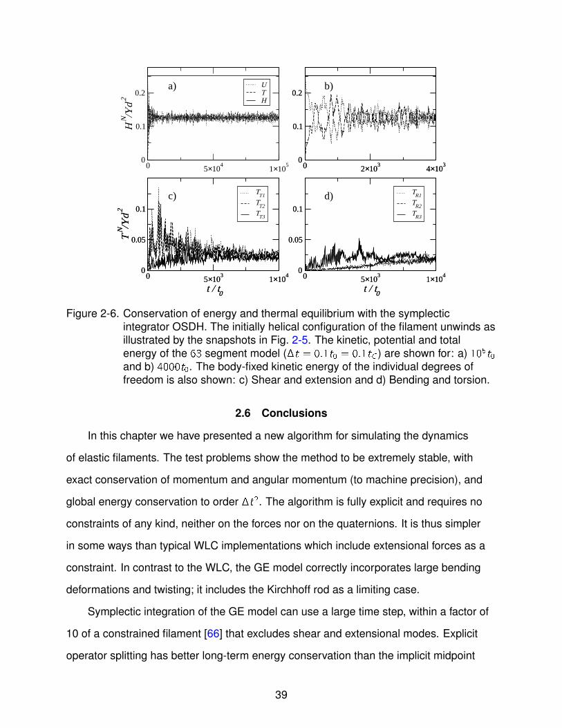
As in the planar bend case, the symplectic algorithm (OSDH) conserves energy,

Fig. 2-6a, for as long a time as we have tested, up to 106t0. The non-linear coupling is

much stronger than in the previous example, because of the higher curvature and the

three-dimensional deformation; here the filament rapidly comes to thermal equilibrium.

The loss of coherent oscillations can be seen more clearly in the expanded time scale

of Fig. 2-6b. Over the same time scale, 104t0, we see that equipartition of energy is

37

Figure 2-5. Filament shapes at different times: a) t = 0; b) t = 100t0; c) t = 200t0; d)t = 300t0; e) t = 400t0; f) t = 500t0. The simulations with 630 segments areshown as thick solid lines, while simulations with 63 segments are shown bythe spheres.

established between the various degrees of freedom, Figs. 2-6c and 2-6d; similar

results holds for the various components of the potential energy as well. Unlike the

planar bend case, here the more finely resolved filament (630 segments) comes to

thermal equilibrium on more or less the same time scale, ∼ 40, 000t0, rather than

106t0 as would be expected for a quadratic scaling of the equilibration time with N. This

suggests fundamental differences in the dynamics of the two-dimensional bending from

the full three-dimensional problem.

38

0 2×103

4×103

0

0.1

0.2UTH

0 5×104

1×105

0

0.1

0.2

HN /Y

d2

a)

0 5×103

1×104

t / t0

0

0.05

0.1

TR1

TR2

TR3

0 5×103

1×104

t / t0

0

0.05

0.1

TN /Y

d2

TT1

TT2

TT3

0 2×103

4×103

0

0.1

0.2b)

0 5×103

1×104

t / t0

0

0.05

0.1

TN /Y

d2

c)

0 5×103

1×104

t / t0

0

0.05

0.1

d)

Figure 2-6. Conservation of energy and thermal equilibrium with the symplecticintegrator OSDH. The initially helical configuration of the filament unwinds asillustrated by the snapshots in Fig. 2-5. The kinetic, potential and totalenergy of the 63 segment model (�t = 0.1t0 = 0.1tC ) are shown for: a) 105t0

and b) 4000t0. The body-fixed kinetic energy of the individual degrees offreedom is also shown: c) Shear and extension and d) Bending and torsion.

2.6 Conclusions

In this chapter we have presented a new algorithm for simulating the dynamics

of elastic filaments. The test problems show the method to be extremely stable, with

exact conservation of momentum and angular momentum (to machine precision), and

global energy conservation to order �t2. The algorithm is fully explicit and requires no

constraints of any kind, neither on the forces nor on the quaternions. It is thus simpler

in some ways than typical WLC implementations which include extensional forces as a

constraint. In contrast to the WLC, the GE model correctly incorporates large bending

deformations and twisting; it includes the Kirchhoff rod as a limiting case.

Symplectic integration of the GE model can use a large time step, within a factor of

10 of a constrained filament [66] that excludes shear and extensional modes. Explicit

operator splitting has better long-term energy conservation than the implicit midpoint

39

method and requires an order of magnitude fewer force evaluations per time step. In

cases where the time step is limited by the stiffness of excluded volume interactions, the

GE model may be more computationally efficient than the Kirchhoff model, due to the

absence of constraints.

In this work we only discussed Hamiltonian systems, but operator splitting is a

powerful method for integrating stochastic systems as well [78, 79]. We have considered

the case when the rod is subjected to dissipative and random forces, in addition to the

elastic forces. Using operator splitting we can integrate the momentum equation exactly,

using the Ornstein-Uhlenbeck solution, and therefore preserve quadratic norms to order

�t2, as opposed to the �t accuracy of Brownian dynamics. This work will be reported in

a future work.

40

CHAPTER 3MECHANICS OF VORTICELLA

3.1 Introduction

Relative to its size, Vorticella convallaria is one of the fastest moving organisms

on the planet [83]. Its cell body is tethered to a substrate by a slender stalk which coils

up into a helix in order to move the body (Fig. 3-1a-b). A thin, elastic structure called

spasmoneme, enclosed within the cell membrane, winds helically inside the stalk close

to its outer sheath [84, 85]. Spasmoneme generates an ATP-independent [86, 87]

tensile force in response to calcium signaling, which drives the coiling of the stalk [88].

The cell body contains calcium storage sites in the endoplasmic reticulum [89], which

release Ca2+ ions spontaneously or in response to an external stimulus [90]. The signal

is propagated down the spasmoneme by calcium-induced-calcium-release (CICR)

from calcium storing membranous tubules within the spasmoneme [85, 89, 91, 92]. In

this mechanism, tubules release the stored calcium upon permeabilization by a small

external calcium concentration. In-vivo experiments [91] show that a Ca2+ concentration

as small as 10−7 M is sufficient to trigger the release of stored calcium. A permeabilized

tubule provides a sharp increase in the local Ca2+ concentration, which triggers further

calcium release from the surrounding tubules. Thus, an initial calcium signal generated

in the cell body can propagate through the stalk by successive permeabilization of the

pre-existing calcium tubules in the spasmoneme – a diffusion cascade similar to what is

observed in muscle cells [93].

The released Ca2+ ions bind to a 20 kDa calcium-binding protein called spasmin,

which constitutes 40 to 60% of the spasmoneme dry mass [94, 95]. As a result, a state

of tension is induced in the spasmoneme which drives its contraction with a maximum

speed of about 6 cm s−1 (Fig. 3-1e) and a tensile force up to 500 nN (S. Ryu, MIT,

personal communication, 2009). Since the spasmoneme winds helically inside the stalk,

the contraction collapses the straight stalk into a helix, which is similar to the mechanics

41

Figure 3-1. a-b) Images of V. Convallaria in extended and contracted states [97]. c-d)The model in extended and contracted states. The head is modeled by anincompressible sphere, the stalk by an elastic rod (in gray) and thespasmoneme by a thin fiber (in black) winding helically around the stalk. e)A typical velocity profile of the cell body is shown from the time when themotion starts; the graph was redrawn from Fig. 2 of Ref. 98. The scale barin panel a–d is 50 µm.

of some coiling bateria [96]. The reverse process (recovery) is powered by dissociation

of Ca2+ ions from spasmin and active sequestration back into the calcium storage sites.

Although the general causes of contraction and recovery are known, the mechanics

of the coiling process and its rate limitations are not well understood. In this work we

have coupled a computational model for the mechanical aspects of Vorticella contraction

and recovery with a kinetic model for calcium binding. Simulations capture several

features of the experimental observations, including the velocity profile (Fig. 3-1e), the

42

scaling of the peak velocity with viscosity, and the shape of the fully contracted stalk.

Furthermore, the experimentally observed shapes of the collapsing and recovering

stalk can only be reproduced if the Young’s modulus of the stalk lies in a narrow range

around 1 kPa. Our simulations suggest that the recovery process of the organism is

driven by the bending energy of the coiled stalk, at a rate controlled by the dissociation

of the calcium-spasmin complex. By identifying geometric constraints applicable

to the stalk-spasmoneme system we can explain the connection between the final

configuration of the stalk and the rotation of the cell body. We have determined that the

rate of contraction of the stalk is controlled by calcium-spasmin binding kinetics, as well

as by the speed of the calcium signal.

3.2 Model and Simulations

3.2.1 Mechanical Model

Our mechanical model for Vorticella, Fig. 3-1c, contains three components: i) the

cell body, also referred to as the “head” ii) the stalk and iii) the spasmoneme. The head

acts as a source of inertia and viscous drag, and its shape is approximated by a rigid

sphere. The translational drag acting on a sphere at time t is given by [99]

Fd = 2πR3[ρ

3∂u∂t

+3ηuR2 +

3R

(ρηπ

)1/2∫ t

0

∂u∂τ

dτ(t − τ)1/2

], (3–1)

where ρ and η are the mass density and dynamic viscosity of the fluid, R and u are the

radius and velocity of the sphere, and t is the time. The first term in Eq. 3–1 accounts

for the added mass from the rapidly propagating pressure waves, the second term is

the Stokes drag, and the last term is due to the diffusion of vorticity in the fluid. The

rotational drag on a sphere relaxes faster than the translational drag [99], and we take

only the Stokes contribution to the rotational friction, 8πR3η.

The stalk is a pliable slender structure, which bends into a helical shape during

contraction of Vorticella and recovers its original shape following the removal of calcium.

It is modeled as a homogenous elastic rod with six degrees of freedom - two shears, an

43

extension, two bends and a twist. The equations of motion for an over-damped elastic

rod are

∂sF = ξT .u, (3–2)

∂sM + t× F = ξR .ω, (3–3)

where F and M are the elastic force and moment acting on the rod, u and ω are the

translational and rotational velocities, t is the tangent to the centerline of the rod, and

ξT and ξR are the translational and rotational friction per unit length. In a frame aligned

with the tangent vector, the friction matrices are diagonal and in the slender-body

approximation [100, 101],

ξT =4πη

ln(2A)

1 0 0

0 1 0

0 0 0.5

, (3–4)

ξR = πηd2

1 0 0

0 1 0

0 0 0.68

, (3–5)

where d is the diameter and A is the aspect ratio of the rod. The precise values of

the friction coefficients are not important because the drag on the stalk is small in

comparison with the drag on the head. Simulations confirm that the dynamics remain

unaffected if ξT and ξR are varied by a factor of four. Further details of the model can be

found in Ref. 4.

The spasmoneme contracts in the presence of free calcium ions, and exerts forces

and couples on the stalk that bend it into a helix. We assume that the spasmoneme

does not offer any bending resistance but only generates a tension along its length.

Hence, it is modeled by an elastic fiber attached helically around the stalk.

44

Figure 3-2. A segment of the rod-fiber assembly showing the tension (T) in the fiber andits position relative to the centerline of the rod. The segment length in thediscretized model is given by ls = L/Ns where L is the length of the rod andNs is the number of segments. The force acting on the centerline (Fs) isparallel to T and exerts shear and compressional forces. The moment (Ms)of the tension is perpendicular to r and Fs , and generates bend and twistcouples. The rest length of the spasmoneme segment in its calcium-freestate is le and its rest length in the calcium-bound state is lc ; its timedependent length, l , varies between le and lc . The force and couple actingon the bottom plane are not shown.

What happens at the molecular level when calcium binds to spasmoneme is not

known. However, from a mechanistic point of view, it is sufficient to assume that the rest

length of spasmoneme decreases significantly upon calcium binding. As the calcium

signal traverses successive parts of the spasmoneme, the local rest length decreases,

resulting in contractile force generation. We define the rest length of a spasmoneme

segment in its calcium-free state as le , and its rest length in the calcium-bound state as

lc ; its time dependent length, l , varies between le and lc as illustrated in Fig. 3-2.

The force-extension relationship of the Zoothamnium spasmoneme has been

reported to be non-linear [102], and it may be non-linear for Vorticella spasmoneme as

well. However, in the absence of experimental data, we assume a linear relationship

between the tensile force and the extension of the spasmoneme. The local tension

45

vector in a spasmoneme segment (Fig. 3-2) is given by

T = κ(γ − γc )l, (3–6)

where γ = l/le is the tensile strain and γc = lc/le is the strain in the reference

configuration; κ is the extensional stiffness and l is a unit vector in the direction of

the fiber. Before calcium binding γc = γ = 1, but γc decreases in response to an

increase in the local concentration of calcium-bound spasmin. This generates a force

that drives l from le to lc . The force and couple exerted by the fiber on the axis of the rod

are given by

Fs = T, (3–7)

Ms = r × Fs , (3–8)

where r is the vector from the rod axis to the fiber (Fig. 3-2). The force, Fs , and the

couple, Ms , are added to the elastic forces and moments of the rod, ∂sF and ∂sM

(Eqs. 4–1 and 4–2).

3.2.2 Chemical Model

Spasmin has been shown to carry two functional calcium-binding (EF-hand)

domains [103], which occur in several calcium-binding proteins [104]. The association of

free calcium ions to a binding site, S , on a spasmin protein is modeled by second order

kinetics,

S + Ca2+ ­ C , (3–9)

where C represents the Ca2+–EF-hand complex. The rate equation for the reaction,

d [C ]dt

= k[S ][Ca2+]− k−1[C ], (3–10)

46

is subject to constraints on the total number of binding sites, [ST ], and calcium ions,

[Ca2+T ],

[ST ] = [S ] + [C ], (3–11)[Ca2+

T]

= [Ca2+] + [C ], (3–12)

and the initial condition

[C ](t = 0) = 0. (3–13)

The local reference strain of the spasmoneme in the calcium-bound state, γc , is

assumed to be linearly related to the local concentration of the complex, [C ],

γc (t) = 1− (1− γ∞c )[C ](t)[ST ]

, (3–14)

where the parameter γ∞c is defined as the strain of the calcium-saturated spasmoneme.

Initially [C ] = 0 and γc = 1; when the binding sites are saturated [C ] = [ST ] and γc = γ∞c .

Propagation of the calcium signal is modeled by a constant velocity front that

travels down the spasmoneme, triggering the onset of the calcium binding reaction at

successive segments.

3.2.3 Geometric Constraints

If we assume that the stalk and spasmoneme are attached, then there are

geometric constraints relating the initial straight configuration and the final helical

configuration. The length of the stalk in the helical configuration is

L = Nf ((πD)2 + P2)1/2, (3–15)

where Nf is the number of turns in the helix, D is its diameter and P is its pitch. The

helix formed by the spasmoneme has the same pitch and number of turns as the

stalk, but its diameter is D − 2r , where r is the distance of the fiber from the rod’s axis

47

(Fig. 3-2); its length is given by

Lc = Nf ((π(D − 2r ))2 + P2)1/2. (3–16)

The equations can be simplified because the pitch, P ∼ 3.5 µm (Fig. 3-1b), is small

in comparison to the perimeters, πD ∼ 17 µm and π(D − 2r ) ∼ 10 µm; omitting terms in

P2 from the Eqs. 3–15 and 3–16,

Nf =L− Lc

2πr, (3–17)

D =2rL

L− Lc. (3–18)

It is significant, and somewhat counter intuitive, that the number of turns in the final

contracted helix is independent of the initial number of turns the spasmoneme makes

around the stalk. Instead, Nf depends primarily on the extent of contraction, Lc , which

we have confirmed with simulations.

High resolution images of Vorticella [97] have been used to estimate the lengths

of the fully extended and contracted spasmoneme, Le and Lc . The images, reproduced

by permission in Fig. 3-1, were used to measure the dimensions of the extended stalk,

L and d , and the geometry of the contracted spasmoneme, Nf , D − 2r , and P. We

then calculated Lc from Eq. 3–16 and Le from the equivalent relation for the helical

spasmoneme in the fully extended stalk,

Le = ((2πrNi )2 + L2)1/2; (3–19)

Ni is the initial number of turns of the spasmoneme around the straight stalk and r ≈d/2. On comparing Lc with Le , we conclude that the spasmoneme has shrunk to about

a quarter of its length, which is consistent with estimates based on the configuration of

the helical stalk, Eqs. 3–17 and 3–18. The spasmoneme of Carchesium, a relative of

Vorticella, has been reported to contract to about a third of its length [84], so shrinkage

of Vorticella spasmoneme to a quarter of its length is not unreasonable. We assume the

48

contraction ratio, Lc/Le = 0.25, to be an intrinsic property of Vorticella spasmoneme,

valid locally as well as globally. Therefore the reference strain in the calcium saturated

state, γ∞c , is taken to be 0.25.

The predictions of the constraints (Eqs. 3–17 and 3–18) can be compared with

the images in Figs. 3-1a-b. The length of the contracting part of the stalk, L, is ∼ 100

µm, the average stalk-spasmoneme distance, r , is ∼ 2 µm, the initial length of the

spasmoneme, Le , is ∼ 112 µm (Eq. 3–19) and its contracted length, Lc , is 28 µm

(= Le/4). Using Eqs. 3–17 and 3–18 we get Nf = 5.7 turns and D = 5.6 µm while the

observation is Nf ∼ 4.5 and D ∼ 5.9 µm.

A further consistency check on the geometry of the final helix can be obtained

from Eqs. 3–15 and 3–16, including the contribution from the pitch. There are three

unknowns (P, D, and Nf ) and only two equations, but real values of P require

r >D2

(1− Lc

L) & 0.36D. (3–20)

The experimentally observed diameter, D = 5.9 µm, lies outside this range when r =

d/2 = 2 µm. However, it is evident from the higher magnification images of the helical

stalk (Fig. 3-1b) that it has been squeezed into an oval shape by the spasmoneme and,

as a result, the distance between the stalk axis and the spasmoneme, r , has increased.

Hence, the geometric constraints correctly imply a squeezing of the stalk as well.

3.2.4 Parameter Estimation

3.2.4.1 Geometric and mechanical parameters

There are several geometric parameters required to describe the Vorticella model;

these can be estimated from published images and are listed in Table 4-1. The stalk

diameter and length vary from source to source but the aspect ratio (L/d) remains close

to 30. The strain at saturation is obtained from the fully contracted and the fully extended

lengths as γ∞c = Lc/Le ; Lc and Le are the macroscopic equivalents of the segment

lengths lc and le shown in Fig. 3-2.

49

The parameters describing the mechanical properties of the stalk, the spasmoneme

and the surrounding medium are listed in Table 4-2. The tension in the spasmoneme

was deduced by fitting a linear force-extension relation (Eq. 3–6) to the available data on

the maximum force, Fmax , generated by a fully extended spasmoneme. The force will be

maximum when the length of the spasmoneme is at its maximum, γ = 1, while its rest

length is at its minimum, γc = γ∞c . The maximum force for in-vivo measurements,

Fmax = κ(1− γ∞c ), (3–21)

ranges from 200 nN [105] to 500 nN (S. Ryu, MIT, personal communication, 2009). We

take Fmax = 300 nN and γ∞c = 0.25 which gives κ = 400 nN. The extensional modulus

of spasmoneme estimated from κ is ∼ 100 kPa which is two orders of magnitude larger

than the Young’s modulus of the stalk (estimated later). Simulations show that if the

spasmoneme is significantly stiffer than the stalk, small variations in κ (up to 25%) do not

alter the dynamics significantly.

Micrographs of contracted Vorticella indicate no apparent shrinkage in the stalk

length under maximum contraction, suggesting that the extensional modulus, Ye , of the

fluid filled stalk is significantly larger than the maximum compressive stress exerted by

the spasmoneme. Simulations confirm that any value of Ye > 25κ/d2 ≈ 400 kPa yields

the same contraction dynamics. We have used Ye = 1 MPa for the results shown here.

The extensional modulus of a Carchesium stalk is similar, around 400 kPa [106]. We

have found that the extensional modulus, Ye , is few orders of magnitude larger than the

Young’s modulus that appears in the bending stiffness, YI . We think this is because the

fluid-filled gel inside the sheath resists change in volume but has little shear resistance.

The bending stiffness of the stalk determines the elastic resistance of the

contracting stalk relative to the viscous drag from the head, which sets the viscosity

range where power limited contraction is observed [98]. Furthermore, the bending

energy stored in the coiled stalk, ∼ YIL/D2, is responsible for recovery of the

50

organism from the contracted state. Thus, the range of values for Y can be bounded by

comparison with experimental observations of contraction and recovery. Here we have

assumed that the moment of inertia of the stalk is I = πd 4/64.

The shear modulus of the stalk, G , is related to the Young’s modulus,

G =Y

2(1 + σ), (3–22)

where σ is Poisson’s ratio, which we take to be 0.5. The dynamics of collapse and

recovery are insensitive to changes (two fold) in the value of G and its exact value is

immaterial for our purposes. A viscosity of 1 cP is assumed for the medium (water),

except when glycerine is added to increase the viscosity.

It is evident from Fig. 3-1b that the stalk is squeezed into an oval shape by the

contraction, leading to an increase in the distance between the stalk axis and the

spasmoneme, r . As suggested by the geometric relations, our simulations confirm that

this slight increase in r is important in order to explain the observed configuration of the

collapsed stalk. We increased r in proportion to the local calcium–EF-hand complex

concentration, [C ], from an initial value of 0.45d to a final value of 0.65d in order to

capture the squeezing of the stalk.

A small part of the stalk shown in Fig. 3-1b remains uncoiled for reasons unknown

to us. Simulations show that keeping the spasmoneme uncontracted in a small length

(∼ 10 µm) next to the tethered end, leaves the corresponding length of the stalk uncoiled

(Fig. 3-1d).

3.2.4.2 Chemical parameters

The dissociation constant, Kd , of the calcium–EF-hand complex, C , has been

independently estimated to be ∼ 10−6.5 M [109]. The forward rate constant, k , was

obtained by fitting the simulated velocity profile (discussed later) to experimental

observations; it is the only directly fitted parameter in our model. The backward rate

constant, k−1, is given by kKd ≈ 0.15 s−1. The calcium-binding-site concentration, [ST ],

51

Table 3-1. Geometric parameters from images of Vorticella. The range of parametersencompasses the data in Refs. 84, 85, 97, 98, 107, 108, including the imagesin Figs. 3-1a-b. The values used in the simulation were taken from Ref. 98where velocity data for the contraction was reported.

Parameter Symbol Range Value

Stalk diameter d 3− 6 µm 5 µm

Head diameter dh 8− 11d 50 µm

Stalk length L 25− 30d 150 µm

Initial turns of spasmoneme Ni ∼ 1 per 25 µm 6

Stalk-spasmoneme distance r ∼ d/2 2.5 µm

Uncontracted spasmoneme length Le ((2πrNi )2 + L2)1/2 177 µm

Contracted spasmoneme length Lc ∼ Le/4 44 µm

Strain at saturation γ∞c Lc/Le 0.25

Table 3-2. Mechanical parameters. These parameters are material properties and areindependent of the size of the organism.

Parameter Symbol Value Source

Spasmoneme stiffness κ ∼ 400 nN Maximum force [105]

Stalk extensional modulus Ye ∼ 1 MPa Incompressibility

Stalk Young’s modulus Y ∼ 1 kPa Simulations

Stalk shear modulus G ∼ 0.33 kPa Elasticity relations

Medium viscosity η 1 cP Viscosity of water

Table 3-3. Chemical parameters

Parameter Symbol Value Source

Dissociation constant Kd ∼ 10−6.5 M Refs. 109, 110

Binding rate constant k 5.105 M−1s−1 Simulations

Dissociation rate const. k−1 ∼ 0.15 s−1 Thermodynamics (= kKd )

Total binding sites conc. [ST ] ∼ 8 mM Ref. 94

Total calcium conc. [Ca2+T ] ∼ 8 mM Binding site conc.

Ca2+ signal speed VCa ∼ 10 cm s−1 Ref. 98

52

is not known for Vorticella; we estimate a value of 8 mM from in-vitro experiments with

Zoothamnium, which show that about 0.34 gram of calcium per kg of wet spasmoneme

saturates all binding sites [111]. Assuming a density of 1.1 kg/l for wet spasmoneme,

yields a value of about 8 mM for [ST ]. No direct measurement of in-vivo calcium

concentration, [Ca2+T ], is available. However, [Ca2+

T ] cannot be significantly less

than [ST ] because the maximum force measured in calcium saturation experiments

[109] is less than what is observed in in-vivo experiments [105], which suggests that

the spasmin is saturated by calcium. [Ca2+T ] is not likely to be significantly larger than

[ST ] because Vorticella has to work to sequester the released Ca2+ ions back into the

calcium storing tubules. Hence, we assume [Ca2+T ] ≈ [ST ]. The speed of the calcium

signal, VCa = 10 cm s−1, is taken from experimental observations [98].

3.3 Results

3.3.1 Fast Binding

We will first treat the case where the calcium binding reaction is not rate limiting,

resulting in an instantaneous force (γc = γ∞c ) in those parts of the spasmoneme where

the signal has propagated. We will later show that a finite binding rate must be assumed

in order to capture the experimentally observed dynamics.

The stalk-substrate attachment is modeled by a clamped boundary condition (no

translation or rotation) at one end of the stalk. The other end bears the head and is

free to translate and rotate. Initially the stalk is straight with the spasmoneme winding

helically around it. A signal travels down the spasmoneme from the head bearing end,

with a constant speed of 10 cm s−1. The spasmoneme experiences an instantaneous

decrease in the local reference strain (γc = γ∞c ) as the signal traverses each segment,

generating a tensile force (Eq. 3–6), as illustrated in Fig. 3-2. The head gets pulled

downwards and the lower part of the stalk, where the signal has not yet reached,

is pulled upwards. Snapshots of the simulations for two Young’s moduli are shown

in Fig. 3-3. For Y = 1 kPa, we can see that the lower part of the stalk undergoes

53

Figure 3-3. Time lapse images of the initial phase of contraction driven by a propagatingcalcium signal; the head is not shown for clarity. Top: Young’s modulus,Y = 1 kPa. Bottom: Y = 4 kPa.

significant deformation while the signal is still in the upper part (t ∼ 1 ms), which is

contrary to experimental observations. On the other hand, for a stiffer stalk, Y = 4 kPa,

the lower part remains essentially at rest until the signal reaches it.

It has been observed that the maximum velocity of the head scales with viscosity

as η−0.5, which implies that most of the energy from spasmoneme contraction is spent

in overcoming the viscous drag [98] rather than bending the stalk. Figure 3-4a shows

the peak velocity plotted against viscosity for Y = 1 and 4 kPa. At lower viscosities (∼ 1

cP), the peak velocity follows experimental scaling if Y ≤ 1 kPa, but for Y = 4 kPa there

is a significant deviation. Hence the upper bound on the bending rigidity of the stalk is

between 1 and 4 kPa.

54

Figure 3-4. Simulation results for contraction driven by a propagating calcium signal. a)Peak velocity vs. viscosity. Solid line indicates a slope of −0.5. b) Velocityprofiles. The peak velocity decays more rapidly than the experimental datashown in Fig. 3-1e. For the stiffer stalk (Y = 4 kPa) the velocity increasesmuch too rapidly as well.

Velocity profiles of the simulations shown in Fig. 3-3 are plotted in Fig. 3-4b.

For Y = 1 kPa, the velocity peaks at 8 cm s−1 and then drops to 1 cm s−1 within a

millisecond. For Y = 4 kPa, the velocity peaks at 5 cm s−1 but with a very different

profile. Neither of these profiles captures the delayed build up and slow decay of the

velocity shown in Fig. 3-1e. We propose that the additional time scale indicates delayed

calcium-spasmin binding kinetics.

3.3.2 Delayed Binding

Velocity profiles for different values of the binding rate constant, k , are shown in

Fig. 3-5a. Simulations with k = 5× 105 M−1s−1 quantitatively reproduce the experimental

data (Fig. 3-1e) including the overall shape, peak velocity (6 cm s−1) and peak position

55

Figure 3-5. Results for Young’s modulus, Y = 1 kPa and different values of rateconstant, k . a) Velocity of the head vs. time. b) Position of the head vs. time.

(2 ms). The time dependent position of the tip of the stalk, shown in Fig. 3-5b, is also in

good agreement with the experiment. The shape of the velocity profile is sensitive to the

calcium-binding rate constant; other values of k do not fit the observations (Fig. 3-5).

Snapshots of a simulation with k = 5 × 105 M−1s−1 and Y = 1 kPa are shown

in Fig. 3-6. Owing to the delayed binding, the stalk remains straight until the calcium

signal passes by and the collapse is more uniformly distributed over the stalk. This is

closer to the observed shapes of the contracting stalk than the simulations assuming

instantaneous binding (cf. Fig. 3-3).

The velocity profiles for different fluid viscosities are shown in Fig. 3-7a. The

peak position is relatively insensitive to the viscosity and the peak velocity scales

asymptotically as η−0.5 (Fig. 3-7b); both findings are consistent with experimental data

[98]. Moreover, simulations and experiments find similar deviations from η−0.5 scaling at

low viscosity.

56

Figure 3-6. Time lapse images of contraction with Young’s modulus, Y = 1 kPa and rateconstant, k = 5× 105 M−1s−1. The stalk is shown in gray while thespasmoneme is shown in black; the head is not shown for clarity.

Figure 3-7. Velocity data for Young’s modulus, Y = 1 kPa and rate constant, k = 5× 105

M−1s−1. a) Velocity profile for different viscosities. b) Peak velocity vs.viscosity. The solid line depicts the slope of −0.5.

57

Figure 3-8. Recovery simulations with Young’s modulus Y = 0.25 kPa (a1-2) and Y = 1kPa (b1-2). Early stalk shapes are shown in a1 and b1 while a2 and b2 showthe shapes at a later time.

3.3.3 Recovery

The recovery of Vorticella is ATP driven and takes place on a much longer time

scale than contraction. Calcium ions are thought to be sequestered back into the

calcium storing tubules in the spasmoneme using ATP hydrolysis as the energy

source. Several questions regarding recovery have been left unanswered in the current

literature. Is the recovery rate limited by Ca2+ ion sequestration, by Ca2+ ion dissociation

from spasmin, by the drag on the head or by a combination of these? What’s the role of

the spasmoneme in recovery: is it under compression against the drag forces or under

tension against the stalk’s bending strain? Our simulations address the mechanics

aspects of these questions.

Recovery simulations start with the stalk at rest in the fully contracted helical shape;

its elastic restoring forces are balanced by the tension in the spasmoneme. To start

recovery, the tension in the spasmoneme is reduced uniformly along its length, at a rate

similar to the rate of recovery observed in the living organism (∼ 0.2 s−1). Simulations

with different bending stiffnesses of the stalk are shown in Fig. 3-8. For a small Young’s

modulus, Y ≤ 0.25 kPa, the stalk uncoils without moving the head significantly (Fig. 3-8

a1-a2), which is contrary to experimental observations. However, for stiffer stalks, Y ≥ 1

kPa, the head is pushed up in the observed fashion (Fig. 3-8 b1-b2). Hence the lower

bound on the Young’s modulus of the stalk is between 0.25 and 1 kPa. We simulated

58

recovery with an enhanced rate of reduction of the tension in the spasmoneme, to show

what would happen if the Ca2+ dissociation and sequestration was faster by an order of

magnitude. Simulations show that even a stiffer stalk, Y = 2 kPa, uncoils without moving

the head, and exhibits shapes similar to those shown in Fig. 3-8a. Hence, chemistry

must control the rate of recovery rather than viscous drag.

The molecular mechanism for force generation by calcium-spasmin binding is not

known and what happens upon calcium unbinding is also unclear. There has been

speculation in the literature that the recovery is driven by the stalk [109] or by the

spasmoneme [87], but no one has demonstrated either case to be true. It is possible

that upon calcium unbinding, the rest length of the spasmoneme increases so rapidly

that it starts exerting an extensional force on the stalk. In this case, the recovery will

be driven by the spasmoneme rather than the stalk. We simulated this mechanism

of recovery and found that for a realistic rate of recovery, the spasmoneme never

develops a compressive force, because the stalk always uncoils fast enough to keep the

spasmoneme under tension. Hence, our simulations indicate that recovery is driven by

the elastic energy stored in the coiled stalk.

3.4 Discussion

Our model of Vorticella contraction yields a number of insights that are not obvious

from the experiments. The geometric analysis shows that the final number of turns in

the helical stalk is independent of the initial number of turns of the spasmoneme around

the stalk. The difference between the initial and final number of turns is made up for by

rotation of the head, since the other end is fixed. Most images of Vorticella show that

the initial number of turns of the spasmoneme is quite close to the final number of turns

of the helical stalk, and that the rotation of the head is small [97, 98, 112]. Since the

number of turns in the contracted state is independent of the initial number of turns of

the spasmoneme, it is interesting that the two end up being so close. Perhaps nature

59

has evolved the organism in such a way that the initial and final number of turns are

similar and the stalk-body junction does not have to bear large torsional strains.

The effective Young’s modulus of the stalk must be close to 1 kPa; otherwise the

experimentally observed contraction and recovery cannot be explained. The Vorticella

stalk has fine slender structures on its surface called Batonnets which wind around the

stalk with the same pitch as the spasmoneme but opposite handedness [84]. Since they

always lie on the outer side of the helix, oriented parallel to the local centerline, their

supposed function is to provide extra bending stiffness to the stalk. A simple deflection

experiment may therefore underpredict the effective bending stiffness during collapse

and recovery. Simulations predict that when the organism recovers from its contracted

state in a high viscosity fluid (∼ 20 cP), the stalk will uncoil without significant motion

of the head; later the bent stalk will gradually straighten, as seen in Figs. 3-8a1-2. This

prediction could be used to test our estimate of Y = 1 kPa.

The collapse of the stalk (six fold) is larger than the reduction in length of the

spasmoneme (four fold). Simulations show that the collapsing stalk forces the

spasmoneme into a helical coil, thereby increasing the tension in the spasmoneme

and generating additional force for contraction.

It has been suggested that an action-potential induces calcium release in the Vor-

ticella spasmoneme [98]. However, the observation that membrane depolarization

occurs after cellular contraction [113] argues against an action-potential driven

signal. The observed signal speed (10 cm s−1) can in fact be explained by the

calcium-induced-calcium-release (CICR) mechanism, as shown in the Appendix,

contrary to what has been suggested previously [98]. However, a CICR signal cannot

entirely explain the dynamics of the collapsing stalk; there must be an additional delay

which we propose comes from the calcium-spasmin binding kinetics.

60

Simulations show that recovery is driven by the bending energy stored in the coiled

stalk, at a rate limited by calcium dissociation and sequestration. A dissociation time of 7

s, as calculated from (k−1)−1, is consistent with experimentally observed recovery.

The simulations offer some unexpected insights into the contraction mechanics.

While the signal is still in the upper part of the stalk, tension in the spasmoneme pulls

the head downwards and the lower part of the stalk upwards, thereby storing strain

energy in the stalk-spasmoneme segments that have not yet been triggered by calcium.

The effect is magnified by the inertia of the intially stationary fluid around the cell body

(Eq. 3–1) and depends on the head size. When the signal reaches the lower region,

stored strain energy is quickly converted into kinetic energy of the head, which brings

about a sudden rise in the velocity. The model predicts that for long stalks (L & 150 µm),

there will be a plateau in the velocity profile before the maximum velocity is reached,

as in Fig. 3-1e, which will be missing for short stalks (L . 75 µm). The rise to the peak

velocity will be steeper for long stalks than for short ones.

It is evident that the spasmoneme exerts a local tension along the whole length

of the stalk. Nevertheless, the assumption that the spasmoneme is rigidly bound to

the stalk along its entire length may not be entirely correct. The micrographs [84, 85]

and spasmoneme extraction experiments [102, 109] suggest that it simply occupies a

helical cavity inside the stalk’s fibrillar matrix. Thus, it might be able to acquire some

twist without twisting the stalk, an effect we have neglected in our geometric analysis.

The spasmoneme also has a significant cross section in comparison to the stalk,

unlike the thin fiber modeled here. Hence, it might contribute asymmetrically to the

bending stiffness of the stalk. We have not considered cooperative binding of calcium

and spasmin [109, 114] in our kinetic model, for lack of experimentally measured

rate constants. However, we have been able to explain the observed velocity profile

reasonably well, which suggests that cooperative binding does not play a critical role in

the dynamics of the organism.

61

The main conclusions drawn from this model are as follows. The contraction of

Vorticella is rate-limited by calcium-spasmin binding kinetics as well as by the signal

propagation speed. Recovery is driven by the elastic energy stored in the coiled stalk,

at a rate controlled by calcium dissociation and sequestration. The effective Young’s

modulus of the stalk is estimated to be about 1 kPa. Vorticella contraction is subject

to geometric constraints, which determine the number of turns in the helical stalk and

the rotation of the head. Finally, the number of turns in the coiled stalk is geometrically

independent of the number of turns the spasmoneme makes around the straight stalk.

62

CHAPTER 4CYTO-MECHANICS OF MICROTUBULAR BUCKLING AND CENTERING OF

CENTROSOME

4.1 Introduction

Despite being fundamental to the understanding of several cellular processes,

cytoskeletal mechanics is poorly understood, primarily due to the multi-scale physical

and chemical complexity of cells. Positioning of the centrosome is central to cytoskeletal

organization and basic processes like migration, division and cell cycles [115, 116].

Positioning of the nucleus has been widely assumed to closely follow the positioning

of the centrosome [117] and is equally critical in cellular processes [118]. A variety

of diseases such as Emery-Dreifuss muscular dystrophy, dilated cardiomyopathy,

and Dunnigan-type familial partial lipodystrophy [119–122] have been traced back

to mutations in proteins (lamin, nesprin etc.) that physically link the nucleus to the

cytoskeleton. Although the molecular mechanism underlying these diseases remains

unknown [123], they may result from abnormal force transmission from the cytoskeleton

to the nucleus [123–125]. Therefore, research on centrosomal and nuclear translation is

scientifically as well as clinically relevant.

Since the nucleus closely follows the centrosome [117], it is imperative to address

the positioning mechanism of the centrosome in order to understand that of the

nucleus. In patterned cells, the centrosome localized at the geometric center of the

pattern [126] as shown in Fig. 4-1. How does the centrosome find the centroid in the

three dimensional body of a cell? The mechanism of centering of the centrosome

is controversial. While it is known that the microtubules (MTs) growing out from the

centrosome mediate the forces acting on it [127], whether the forces on the centrosome

are compressive or tensile is not established. On one hand, MTs growing against the

cell membrane are thought to center the centrosome through pushing forces [21, 128].

On the other hand, immobile dynein motors are implicated to render centering through

pulling forces on the MTs [115, 126, 129].

63

Figure 4-1. Centrosome location in a) unpatterned b) square c) pentagonal bovinecapillary endothelial (BCE) cells. The centrosome is stained in green,nucleus in blue and MTs in red. The arrow in c shows the direction of thevector connecting the center of the nucleus with the centrosome. The scalebars are 5µm in all. Courtesy Dr. Lele’s group.

In this work, we have coupled a computational model for the dynamics of the

microtubular aster with a model for the dynein motors, which are assumed to be tethered

to the cortex at the light-chain end and pulling on the MTs at the heavy-chain end. The

MTs are modeled as elastic filaments growing stochastically from the centrosome and

exhibiting dynamic instability. Simulations capture the observed centering time of the

centrosome and show the role of the motors in the dynamics of the MTs. Buckling of

MTs in a cell is considered as an evidence for existence of compressive forces along

the entire length of the MTs, thereby invoking the pushing mechanism for centrosome

centering. However, we demonstrate that even buckled MTs can be be under tension

64

Figure 4-2. Schematic of the dynein model.

along most of their length and hence can transmit the pulling forces of the dynein motors

to the centrosome.

The experiments described in this chapter were performed by Dr. Lele’s group.

Bovine capillary endothelial (BCE) cells were used in all experiments. A laser ablation

technique was employed for cutting single MTs and dynein motors were inhibited

by transfection of cells with CC1, which is the dynein binding domain of the protein

dynactin, which in turn is a dynein activator and a critical linking protein between dynein

and the cellular cortex. Hence, CC1 competitively inhibits binding of the dynein motors

to the cortex.

4.2 Modeling

4.2.1 MT Model

An MT is modeled as an elastic rod with six degrees of freedom - two shears, an

extension, two bends and a twist. The equations of motion for an over-damped elastic

65

rod are

∂sF = ξT · v, (4–1)

∂sM + t× F = ξR · ω, (4–2)

where F and M are the elastic force and moment acting on the rod, v and ω are the

translational and rotational velocities, t is the tangent to the centerline of the rod, and ξT

and ξR are the translational and rotational friction per unit length. Further details of the

original model can be found in chapter 2.

4.2.2 Dynein Model

A dynein motor is assumed to be attached to the cortex at the light-chain end and

walking on an MT at the heavy-chain end. The dynein-cortex link is modeled as a spring

which stretches as the heavy-chain end walks on the microtubular lattice (illustrated

in Fig. 4-2). Since the motor walks from the (+)-end to the (−)-end along the axis of

the MT, it can exert a force only the tangential direction. We assume the standard

force-velocity relation for dynein motors [130],

vm/vmax = 1− t · f/fmax , (4–3)

where t is the unit tangent vector directed towards the (+)-end, vm is the motor speed at

load f on the motor, vmax is the maximum possible motor speed and fmax is the stalling

load. If the MT moves with a velocity v relative to the cortex, then the rate of increase of

force on the MT is given by [131]

dfdt

= κd (v + vmt), (4–4)

where κd is the stiffness of of dynein-cortex spring. Upon substituting vm from Eq. 4–3

and integrating, we get the instantaneous force on the MT as

f(t) = fmax

(1 +

t · vvmax

)(1− exp

[−κd vmax

fmaxt])

t + κd v · (I− tt)t (4–5)

66

The dynein-cortex bonds are assumed to dissociate with a first order rate ko� (s−1) such

that the probability of a bond to exist at time t is given by P(t) = exp(−ko� t). Thus, the

mean force over the lifetime of a bond is given by

〈f〉 =∫ ∞

0f(t)dP(t) = f0

(1 +

t · vvmax

)t +

κd

ko�v · (I− tt), (4–6)

where

f0 =fmax

(fmax ko� )/(vmaxκd ) + 1(4–7)

is the average force per dynein molecule on a stationary MT in the tangential direction.

Equation 4–6 can be multiplied throughout by the dynein density per unit length, ρ, and

rewritten as

K = F0t− ξ‖T tt · v − ξ⊥T (I− tt) · v, (4–8)

where K is the mean force per unit length exerted by the motors on the MT, F0 = ρf0 is

the tangential force exerted by the motors on the MT, ξ‖T and ξ⊥T are the friction factors

parallel and perpendicular to the microtubular axis given by

ξ‖T =

ρf0

vmax, (4–9)

ξ⊥T =ρκd

ko�, (4–10)

The force exerted by the motors, K, is added to the internal forces of the MT (Eq. 4–1) in

order to simulate the dynamics of motor-driven MTs. Hence, Eq. 4–1 becomes

∂sF + K = 0. (4–11)

4.2.3 Microtubular Dynamic Instability Model

Microtubules exhibit stochastic polymerization and depolymerization. Under

steady state conditions, the depolymerization rate of MTs is about 3 times faster than

the polymerization rate. The stochastic transition from growth to shrinking is called

’catastrophe’, and the reverse stochastic transition from shrinking to growth is called

67

’rescue’ or ’recovery’ [132]. The two phenomena together constitute the ’dynamic

instability’ of MTs. The summed up length of all the MTs in a cell must be limited by the

total amount of tubulin monomers available in the cytosol. The cumulative length of MTs

in the model cell is given by

Ltot =NMT × Lmax

2, (4–12)

where NMT is the total number of MTs (which is kept constant through the simulations)

and Lmax is maximum length a single MT is allowed to acquire due to computational

constraints and it is chosen as twice the size of the square cell. This constraint

on the cumulative length, Ltot , is required to minimize the effect of the artificial

length-constraint, Lmax , imposed by computational limitations. The instantaneous

lengths of all the MTs are added to calculate the total microtubular length at time t given

by,

Lpol (t) =NMT∑

i=1

Li (t), (4–13)

where Li (t) is the instantaneous length of the i th MT. Constraint on the total length of all

the MTs yields the unpolymerized length of MTs as

Lunpol (t) = Ltot − Lpol (t). (4–14)

The frequency of catastrophe events and the rate of polymerization of MTs are

dependent on the concentration of tubulin monomers in the cytosol, while the

frequency of recovery and the rate of depolymerization are independent of the tubulin

concentration [133]. Hence, the catastrophe rate-constant and the polymerization speed

are modeled as

kcat(t) =34

k sscat

Lpol (t)Ltot

+k ss

cat

4, (4–15)

Vpol (t) = 4V sspol

Lunpol (t)Ltot

+ V sspol , (4–16)

68

0 20 40 60 80MT Length (µm)

0.00

0.10

0.20

Frac

tion

of M

Ts

Figure 4-3. Steady state length distribution of MTs resulting from the dynamic instabilitymodel (Eqs. 4–15 and 4–16). Total number of MTs, NMT = 96 and Lmax = 80µm in a cell of size 40 µm (Fig. 4-12).

where k sscat and V ss

pol are the steady-state catastrophe rate-constant and the

polymerization speed (Table 4-1). The numerical factors in Eqs. 4–15 and 4–16 are

employed to obtain a reasonable length distribution of the MTs (Fig. 4-3). At t = 0

when all the MTs are short in length, we have Lpol/Ltot ∼ 0 and Lunpol/Ltot ∼ 1,

hence polymerization speed is higher than the steady state speed by a factor of 5

while the catastrophe rate is lower by a factor of 4. At steady-state, Lpol/Ltot ∼ 1 and

Lunpol/Ltot ∼ 0, which gives kcat = k sscat and Vpol = V ss

pol .

4.2.4 Cell Periphery Model

The periphery of a cell is a flexible membranous structure called the cell membrane,

which can be deformed by microtubular forces. Hence, it is modeled by a soft repulsive

potential given by

U = U0(e−(D/2−|x |)/λ + e−(D/2−|y |)/λ + e−(T/2−|z |)/λ), (4–17)

where x , y and z are the coordinates of a microtubular segment from the center of

the cell, T is the thickness of the cell, D is the side of the square periphery, U0 is the

potential at the periphery, and λ is the decay length.

Although the model-MTs can bend against the model-periphery, they cannot

exhibit buckling because their tips simply slip at the repulsive potential barrier, unlike

69

θ

Normal vector

MT

Periphery

Tangent vector

Figure 4-4. Schematic of the angle of incidence of an MT on the cell periphery. Theangle of incidence, θ, is the angle between the vector normal to theperiphery and the vector tangent to the MT at the point of contact betweenthe MT and the periphery.

observations where the tips are frequently seen to be stuck at the periphery while MTs

polymerize and buckle. An MT could be stuck at the cell membrane due to its tip being

caught in the cortical mesh and hence, unable to slide laterally on the membrane. When

an MT reorients such that the its (+)-end is parallel to the membrane, it becomes free

to slide along the periphery. Sticking is simulated by restricting the lateral motion of the

tip on the periphery but leaving it free to reorient or to move away from the membrane. It

is known that the buckling instability declines rapidly with increasing angle of incidence

[134]. Hence, we have introduced a probability of sticking as a function of the cosine of

the angle of incidence, θ (illustrated in Fig. 4-4), of the MT at the periphery,

p = cos(θ). (4–18)

The centrosome is modeled as a massless point with a large friction coefficient, ξc , and

is connected to the MTs with springs of stiffness κc .

70

Table 4-1. Microtubule parametersParameter Symbol Value SourceMT steady-state polymerization speed V ss

pol 0.1 µm s−1 Refs. 135, 136MT depolymerization speed Vdepol 0.3 µm s−1 Refs. 135, 136MT steady-state catastrophe rate constant k ss

cat 0.05 s−1 Refs. 135, 136MT recovery rate constant krec 0.2 s−1 Refs. 135, 136MT bending stiffness YI 25 pN µm2 Refs. 137MT outer diameter do 25 nm Ref. 138MT inner diameter di 17 nm Ref. 138MT-centrosome spring constant κc 25 nN µm−1 SimulationsNumber of MTs N ∼ 100 Observation

4.2.5 Multiscale Model

The smallest time scale in the rod model is t0 ∼ d/cl , where d is the diameter

of the rod and cl is the speed of sound in the rod. For an MT, d is ∼ 25 nm and cl is

∼ 1000 ms−1, which gives t0 ∼ 25 ps. This is about 14 orders of magnitude smaller than

the centering time of the centrosome, which is a few thousand seconds. Under normal

circumstances it will not be possible to approach the centering time with our rod model.

However, the intracellular viscosity is large enough to highly overdamp the flexural

modes of an MT, drastically slowing down the motion of its centerline. The shear and

extension modes, which are the fast modes in our model, are fully relaxed to equilibrium

regardless of the medium viscosity. Hence, the time scale separation between the slow

and the fast modes is amplified, which permits the use of a projective integration method

[139] to calculate the dynamics over large time scales. Essentially, we integrate the rod

model using small time steps (10 ps) until the shear and extensional modes (fast) relax

(Eq. 4–2 goes to zero) and only the translational velocities (slow) survive (Eq. 4–11).

Then the slow translational velocities are integrated using a large time step (1 µs) in

order to calculate the new position of the centerline. The fast coordinates, director

vectors of the material planes, are not known for the new centerline position but can be

initialized from the last saved configuration because they will again quickly relax to their

71

Table 4-2. Dynein parametersParameter Symbol Value SourceMax dynein force fmax 8 pN Refs. 140Max dynein speed vmax 0.8 µm s−1 Refs. 130Dynein spring contant κd 1 pN nm−1 Refs. 137Dynein-cortex off rate ko� 1 s−1 Nuclear rotation modelDynein density ρ 2 µm−1 Nuclear rotation model

Table 4-3. Miscellaneous parametersParameter Symbol Value SourceMedium viscosity without motors η ∼ 20 Nsm−2 SimulationsStall probability of ⊥ MTs 0.5 ObservationCell size (side) D 40 µm ObservationPotential at periphery U0 1000 pNnm HeuristicsDecay length of potential λ 100 nm HeuristicsRadius of the centrosome Rc 1 µm Assumed

equilibrium value for the new centerline position of the MT. We repeat this sequence

of relaxing the fast modes at pico second time scale followed by integrating the slow

modes at micro second time scale to approach the centering time.

4.2.6 Parameters

The parameters required for the MT model are listed in Table 4-1. The stiffness of

the springs connecting MTs to the centrosome, κc , is chosen such that the centrosome

and the MTs never drift away from each other. As long as κc is high enough to prevent

any separation between the MTs and the centrosome, its exact value does not bear

any significance. The number of MTs was chosen according to the observations made

in BCE cells. Parameters for the dynein model are listed in Table 4-2. The density

of dynein motors, ρ, and the dynein-cortex off rate, ko� , are not known. These two

parameters are taken from a model for nuclear rotation [131], which captures the

rotational dynamics of cellular nucleus quantitatively. Other parameters required

for simulations are listed in Table 4-3. The intracellular viscosity, η, encountered by

MTs in the absence of dynein motors was estimated by comparison of simulations

72

Figure 4-5. Top: bent MTs in dynein-inhibited cells straighten out within a few secondsafter cutting (courtesy Dr. Lele’s group). Bottom: simulation of an MTunfolding from a bent configuration in the absence of motor forces. Theintracellular viscosity, η, encountered by MTs in absence of dynein motorswas estimated by matching the time scale of unfolding with the experimentalobservation (top). Scale bars: 2 µm.

with experiments as shown in Fig. 4-5. Bent MTs in dynein-inhibited cells were cut

and observed to straighten out within a few seconds, which gives us a time scale of

relaxation that can be reproduced in simulations only by a unique value of viscosity,

which was found to be about 20000 times the viscosity of water. The parameters of

the periphery model, U0 and λ were chosen such that it is neither too stiff nor too soft

a barrier. The friction acting on the centrosome is an unknown and unpredictable

parameter. The centrosome can be thought of as a sphere in a viscous fluid but the

network formed by hundreds of MTs connected with the centrosome at their (–)-ends

can potentially trap several cellular organelles thereby increasing the friction acting on

the centrosome by at least few orders of magnitude. We have assumed the centrosome

to be a sphere of radius Rc in a simple viscous medium and hence, the friction acting on

it is given by 6πRcη. The in-vivo polymerization stall force of MTs is not known, however,

we have observed that about 50 % of the MTs stall upon hitting the cell membrane at a

small angle of incidence (θ). Hence, we have introduced a stall-probability of 0.5 for the

MTs approaching the periphery at a small angle of incidence.

73

Figure 4-6. Experimental observation of MTs polymerizing against cell periphery andbuckling. Scale bars: 2 µm. Courtesy Dr. Lele’s group.

4.3 Results

4.3.1 Buckling of Polymerizing MTs Against Cell Membrane

Microtubules have been observed to undergo buckling when polymerizing against

the cell membrane (Fig. 4-6). An interesting feature of this phenomenon is that the

buckles are concentrated at the distal ends of the MTs, close to the cell periphery, while

the rest of the length remains relatively straight. Simulations show that this phenomenon

can be captured by loading the MTs such that an axial force, directed towards the

distal end, acts on them. Dynein motors are known to walk towards the (−)-end of

the MTs, hence they can apply a distal-end directed axial force on the MTs. Figure

4-7 shows two simulations where a single MT is pinned at the (−)-end and allowed to

polymerize at the (+)-end, which is oriented perpendicular to the cell boundary. As

74

Figure 4-7. Simulations of an MT polymerizing against a soft barrier while being pinnedat the other end. The MTs exhibit a short-wavelength buckling pattern inpresence of of dynein motor forces (top) but a long-wavelength pattern inabsence of motors (bottom). Experimental observations (Fig. 4-6) agree withthe short-wavelength buckling pattern. Scale bar: 5 µm.

75

Figure 4-8. Laser ablation of a single MT in control cells. An MT was cut in the middle att = 6 s and was seen to buckle further after cutting. Scale bar: 5 µm.

the tip of the MT reaches the periphery, it gets pinned there with a probability given by

Eq. 4–18. Upon further polymerization, it buckles due to an increasing compressive

stress. The simulation is repeated for two cases: with and without dynein motors.

Without the motors, the entire length of the MT buckles (Fig. 4-7-bottom) in a lower

mode with a wavelength of about 10 µm. With the motors, which pull the MT towards

the periphery, buckling is concentrated close to the (+)-end while the (−)-end remains

taut (Fig. 4-7-top), in agreement with experiments. Also, the wavelength of the buckles is

closer to the observed wavelength of about 3 µm (Fig. 4-6).

4.3.2 Buckling of a Cut MT

The nature of the forces acting on a single MT can be revealed by cutting the MT

and observing its resulting dynamics. As shown in Fig. 4-8, a single MT was cut at 6

seconds after which its distal half was seen to bend further. This can be explained by

the pulling action of dynein motors on MTs. Figure 4-9 shows a simulation where a

straight, fixed-length MT is pinned at the (+)-end and subjected to dynein-motor forces.

The MT buckles in a fashion similar to the buckling of cut MTs seen in the experiments.

The time scale of buckling also agrees with the observation.

4.3.3 Anterograde Movement of Bends

Microtubular bends have been attributed to motor-driven transport of the (−)-ends

of the MTs toward their fixed (+)-ends [141]. The simulation shown in Fig. 4-9 supports

this notion. Figure 4-10 shows a simulation in which an MT is pinned at both ends and

76

Figure 4-9. Simulation of in-vivo laser ablation of a single MT. The dynein motor forcesare shown with the arrows. The MT buckles further as a result of the motorforces, as seen in the experiments (Fig. 4-8). Scale bar: 5 µm.

bent close to the (−)-end. The dynein motor forces drive the bend towards the distal end

of the MT.

4.3.4 Centrosome Centering In-Vivo

The centrosomal position is known to fluctuate around the geometric center of a

cell. Dr. Lele’s group tracked the coordinates of the centrosome in several control BCE

cells and found that the centrosome makes excursions from the center but returns to it

in about 30 minutes, which is the relaxation time of the centrosome. The autocorrelation

function of the centrosomal position is plotted in Fig. 4-11, where a relaxation time of 30

minutes is apparent.

The central theme of our work is to demonstrate a possible mechanism for the

in-vivo positioning of the centrosome and to quantitatively capture its relaxation time.

To this end, we setup a simulation of a square cell (40 µm wide and 1.5 µm high) with

∼ 100 MTs dynamically polymerizing from the centrosome, which is initially placed

77

Figure 4-10. Anterograde propagation of bends in MTs due to dynein motors. Scale bar:5 µm.

0 30 60 90 120Time (min)

-0.2

0.0

0.2

0.4

0.6

0.8

1.0

Rel

ativ

e Po

sitio

n

Positional autocorrelation function

Figure 4-11. Autocorrelation function of centrosome position in control cells. Theobserved centering time is about 30 minutes.

78

Figure 4-12. Time lapse images of simulation of centrosome positioning without dyneinmotors. The cell boundaries are shown in gray, the MTs in black and thecentrosome as the gray bead in the middle of MTs. The cell contains ∼ 100MTs and is square in shape, 40 µm in width and 1.5 µm in height. Thebuckling forces are unable to push the centrosome towards the center in acell of this size.

off-center. In the absence of motor forces, the MTs buckle along their entire length while

they polymerize against the cell periphery, as seen in Fig. 4-12. These buckling MTs

exert a pushing force on the centrosome away from the closest boundary. However, due

to the large friction on the centrosome and the MTs, the centrosome does not move

significantly (Fig. 4-13).

In the presence of motor forces (Fig. 4-14), the MTs exhibit short-wavelength

buckling close the periphery, as observed before (Fig. 4-6). Since the dynein-generated

force on an MT is directly proportional to its length, the resultant of all forces on the

centrosome lies on the side where the MTs are longer. As a result, the centrosome is

driven towards that point in the cell from which all the boundaries are equidistant. The

centrosome reaches the center within 30 minutes (Fig. 4-15) and oscillates there for

79

0 50 100Time (min)

-15

-10

-5

0

5

Posi

tion

(µm

)

XYZ

Figure 4-13. Time course of the centrosome position without dynein motors,corresponding to Fig. 4-12.

Figure 4-14. Time lapse images of simulation of centrosome positioning with dyneinmotors. The cell boundaries are shown in gray, the MTs in black and thecentrosome as the gray bead in the middle of MTs. The cell contains ∼ 100MTs and is square in shape, 40 µm in width and 1.5 µm in height. Thepulling forces bring the centrosome close to the center and keep it there.

80

0 50 100Time (min)

-15

-10

-5

0

5

Posi

tion

(µm

)

XYZ

Figure 4-15. Time course of the centrosome position with dynein motors, correspondingto Fig. 4-14.

the rest of the simulation. Thus, simulations quantitatively capture the positioning of the

centrosome and its relaxation time as observed in the experiments (Fig. 4-11).

4.3.5 In-Vitro Centering of Centrosome by Polymerization Forces

A few in-vitro experiments have been done to demonstrate centering of the

centrosome by polymerization forces [142]. These experiments report that as long

as the MTs do not bend, they can push the centrosome to the center of the artificial

confinement. However, when the MTs get long enough to bend, the centrosome is

pushed off-center.

In order to understand the mechanics of these in-vitro experiments, we set up a

simulation in which MTs polymerize in a small chamber (12 µm wide and 3 µm deep)

while attached to the centrosome, which is initially placed off-center. Since the chamber

is etched in glass, the MTs cannot get stuck at the periphery unlike they can in-vivo.

Hence, the MTs simply slide along the boundaries once they encounter them. In the

experiments, the viscosity of the buffer solution is close to the viscosity of water, which is

81

Figure 4-16. In-vitro dynamics of ∼ 50 short MTs in a square glass chamber 12 µm wideand 3 µm deep [142]. The centrosome is driven to the center by thepolymerization forces and maintained there.

much lower than the intra-cellular viscosity. At such a low viscosity the MTs relax within

microseconds and hence the dynamics are driven at the time scale of polymerization.

We find that as long as the viscosity is low enough to let the relaxation time scale of MTs

be much smaller than the polymerization time scale, the exact value of the viscosity is

immaterial.

Figure 4-16 shows a simulation of the microtubular dynamics in a small glass

chamber. The length distribution of the MTs is chosen such that most of them never

grow longer than 8 µm, hence they never buckle. The centrosome gets pushed away

from the corner but once it reaches the center, the MTs can no longer exert a large

enough compressive force due to the length constraint. As a result, the centrosome can

only oscillate around the center with a frequency of about 1 per minute.

If the MTs are allowed to grow longer, they can buckle in the chamber and push

the centrosome off-center (Fig. 4-17). If the centrosome is near the periphery, the MTs

that grow towards the periphery slip sideways and cannot exert sufficient pushing force

to drive it towards the center. As a result, the centrosome remains situated off-center,

as seen in the experiments [142]. A comparison of the centrosome position in the

82

Figure 4-17. In-vitro dynamics of ∼ 50 long MTs in a square glass chamber 12 µm wideand 3 µm deep [142]. The centrosome is driven to the center and thenoff-center by the polymerization forces.

0 2 4 6Time (min)

-4

-3

-2

-1

0

1

Posi

tion

(µm

)

XYZ

0 1 2 3 4 5 6 7Time (min)

-6

-4

-2

0

2

4

6

Posi

tion

(µm

)

XYZ

Figure 4-18. Time course of the centrosome position in a square glass chamber. a)Short MTs corresponding to Fig. 4-16. b) Long MTs corresponding toFig. 4-17. A polymerization stall force of 10 pN was introduced.

short-MTs case and the long-MTs case is shown in Fig. 4-18. We also find that due

to the low viscosity, the MTs never reach their in-vitro stall force of 10 pN in these

simulations. Hence, simulations with and without a stall force yield similar results

(Fig. 4-19).

83

0 2 4 6Time (min)

-4

-3

-2

-1

0

1

Posi

tion

(µm

)

XYZ

0 1 2 3 4 5 6 7Time (min)

-6

-4

-2

0

2

4

6

Posi

tion

(µm

)

XYZ

Figure 4-19. Time course of the centrosome position in a square glass chamber. a)Short MTs b) Long MTs. Polymerization stall force was not introduced inthese simulations.

4.4 Discussion

Our model of microtubular dynamics offers several insights into the in-vivo

microtubular dynamics and the cytoskeletal mechanics of centrosome centering.

MTs have been considered to be the compression bearing elements of the cytoskeleton

owing to their buckling behavior, due to which it has been assumed that they transmit

compressive forces to the centrosome. However, we have demonstrated that MTs which

are axially loaded can be under tension at their proximal ends while being buckled at

their distal ends (Fig. 4-7). This highlights a mechanism by which buckled MTs can

transmit the dynein-generated tensile forces to the centrosome. Previous studies have

suggested that the viscoelastic nature of the cytoskeleton might be responsible for

the short-wavelength buckling of MTs close to the cell periphery [23]. However, this

hypothesis predicts that the MTs must straighten out when cut, which is contrary to

experimental evidence. We suggest an alternate, dynein-driven mechanism which can

give rise to the short-wavelength buckling pattern.

Additionally, the buckling of cut MTs in control cells (Fig. 4-9) cannot be explained

by a pushing mechanism. The anterograde movement of proximal portions of MTs [141]

also calls for an active mechanism. Both of these observations can be quantitatively

explained by our model (Figs. 4-9 and 4-10).

84

Simulations show that in large cells (the size of BCE cells), buckled MTs cannot

generate enough pushing force to center the centrosome (Fig. 4-12). In smaller spatial

confinements, the MTs encounter the periphery before growing to their in-vivo length of

about a hundred microns. Since the critical buckling force scales as YI/L2, where L is

the length of the MT, shorter MTs can exert a pushing forces several times greater the

longer MTs in large cells. Combined with a low viscosity in the artificial chambers [142],

the pushing forces of short MTs can easily move the centrosome. However, centering

of the centrosome in small glass chambers is critically dependent on two factors: a

viscosity much lower than the cellular viscosity and a length distribution of MTs such that

they grow long enough to reach the periphery but no longer. Neither of these conditions

are met in large BCE cells, which argues against a pushing mechanism for centrosome

centering.

Furthermore, our model quantitatively captures the centering time of the

centrosome and its positional fluctuations. It is remarkable that with the same set of

parameters our model can quantitatively explain the spatio-temporal characteristics

of three different in-vivo phenomena: short-wavelength buckling of MTs polymerizing

against the cell membrane, buckling of cut MTs, and centering of the centrosome.

Additionally, the same parameter set, with the exception of flexible MTs, quantitatively

captures the rotational fluctuations of cellular nucleus [131].

It is evident that an MT is attached to the centrosome at its (−)-ends. Nevertheless,

the assumption that a spring-like link physically connects the MT with the centrosome

may not be entirely correct because such a connection does not fix the orientation of the

(−)-end relative to the centrosome. Since the MTs grow from the centrosome, it might

be more realistic to model the MT-centrosome connection by fixing the position as well

as the orientation of the (−)-end relative to the centrosome.

The main conclusions drawn from this model are as follows. The short-wavelength

buckling of microtubules polymerizing against the cell membrane is due to the

85

(−)-end-directed axial force exerted by cortex-bound dynein motors on the microtubules.

The same force also explains the buckling behavior of cut microtubules in-vivo. The

centrosome is positioned at the geometric center of a cell by these dynein-generated

tensile forces that are transmitted to the centrosome through the microtubular network.

In the absence of dynein motors, the polymerization forces of the microtubules are

unable to center the centrosome in-vivo. It is significant that the model quantitatively

captures all of these phenomena with same set of parameters.

86

CHAPTER 5SUMMARY

This work has demonstrated the applicability of soft matter physics to biological

systems involving slender micro-structures, such as the Vorticella-stalk and microtubular

network. We have shown that the dynamics of these systems can be understood in

terms of the bending and twisting forces of elastic rods. From a modeling perspective,

this work has given a new explicit algorithm to solve the equations of motion of elastic

filaments. The algorithm is stable, constraint-free and conserves momenta and energy

exactly. In addition, it is several times faster than the prevalent algorithms. The idea

of discretizing the continuum Hamiltonian and differentiating it with respect to discreet

positions in order to derive conservative discreet forces can be applied to other systems

like membranes, which are ubiquitous in biological systems.

The mechano-chemical model of Vorticella dynamics allows us to perform

simulations under conditions that would be impossible to realize in actual experiments.

The model fills gaps in our knowledge about the rate-limiting steps of contraction and

recovery, material properties of the stalk and the mechanism of the recovery process

of the organism. The multi-scale model of the microtubular network in a cell answers

several fundamental questions related to the mechanics of centrosome centering and

whether the MTs are under compression or tension in cells?

Due to the active processes in living systems, most life-processes are far from

equilibrium and there is a growing understanding of application of statistical, molecular

and continuum field theories to these systems. A quantitative physical-chemical

study of biological systems is the consequence of the newly found understanding of

the underlying molecular mechanisms. This growth of knowledge gives rise to more

questions such as how does the spatio-temporal organization of structure and control

emerges from simple marcomolecules within a cell. How are complex multicellular tasks

orchestrated across various levels of cellular organization over several generations?

87

How does the cellular orderliness translate to coordination at the organismic level? How

do organisms evolve over time and what’s the role of the environment in the process

at the molecular and continuum scales? Biology demonstrates phenomena which

traditional mechanics has not encountered before, while engineering brings tools to

probe these phenomena at an unprecedented level of detail. Constant intellectual

exchanges between the fields of biology, chemistry and physics are indispensible for

further development of our understanding of life.

88

APPENDIX APROPERTIES OF QUATERNIONS

A quaternion Z = q0 + qx i + qy j + qz k is a complex number with multiplicative

identities

i 2 = j2 = k2 = ijk = −1. (A–1)

We use the notation Z to indicate the quaternion and qa to denote a vector containing

the scalar, q0, and vector, q = [qx , qy , qz ], components of Z. The quaternion algebra,

Eq. (A–1), leads to rules for multiplication that are analogous to the cross-product of unit

vectors:

ij = −ji = k

jk = −kj = i (A–2)

ki = −ik = j

If we then identify i , j , k , with Cartesian unit vectors i, j, k, the multiplication of two

quaternions, Z = q0 + qx i + qy j + qz k and Z ′ = q′0 + q′x i + q′y j + q′z k, can be written, using

the quaternion multiplication rules defined in Eqs. A–1 and A–2, as

Z ¯ Z ′ = q0q′0 − q · q′ + q0q′ + q′0q + q× q′, (A–3)

where ¯ denotes a quaternion multiplication.

A vector u can be rotated by the unitary transformation Z ¯ u ¯ Z−1, where the

multiplicative inverse of a unit quaternion is Z−1 = q0 − q. Applying Eq. A–3 and treating

u as a quaternion with zero scalar component, the rotated vector u′ is given by

u′ = (q20 − q · q)u + 2qq · u + 2q0q× u, (A–4)

and remains a pure vector. The rotation can also be written in matrix form, u′i = diαuα,

with the director vectors that form the rotation matrix diα as given in Eq. T1.2.

89

An infinitesimal change in the directors is given by a rotation δφ:

δdi = δφ× di , (A–5)

with = ∂sφ and ω = ∂tφ. The combination of the original rotation Z and an additional

infinitesimal rotation δZ = 1 + δφ/2 can be found by applying the rotations sequentially,

u′ + δu = δZ ¯ Z ¯ u¯Z−1 ¯ δZ−1 = Z ′ ¯ u¯Z ′−1. (A–6)

The quaternion Z ′ is found by multiplying the two quaternions,

Z ′ = δZ ¯ Z = q0 − q · δφ2

+ q + q0δφ

2− q× δφ

2. (A–7)

Thus, the variation in the quaternion δZ = Z ′ −Z is linearly related to δφ,

δq0

δqx

δqy

δqz

=12

−qx −qy −qz

q0 qz −qy

−qz q0 qx

qy −qx q0

·

δφx

δφy

δφz

. (A–8)

The column vectors in Eq. A–8 define a set of basis vectors in the quaternion space, eαa,

where eαa is the transpose of the matrix in Eq. A–8. These basis vectors are orthogonal

to qa and relate changes in quaternions to rotations about the space-fixed axes,

δφα = 2eαaδqa, δqa =12

eαaδφα. (A–9)

In this work we have used body-fixed rotations, Eqs. 2–21–2–22, for which we need the

basis vectors eia given in Eq. T1.3; they are related to the space fixed basis eαa by the

rotation matrix, eia = diαeαa. The vectors eia or eαa, together with qa, form a complete

basis in the quaternion space.

90

Finally, we obtain the derivatives of the basis vectors quoted in Eqs. T1.4–T1.5. A

variation in the basis vectors di is related to an infinitesimal rotation, Eq. A–5,

δdiα = εαβγδφβdiγ =3∑

j ,k=1

εijk djαδφk = 23∑

j ,k=1

εijk djαekbδqb. (A–10)

The variation in di can also be directly related to constrained variations in quaternions,

δdiα =∂diα

∂qa(δab − qaqb) δqb, (A–11)

where the projection operator (δab − qaqb) is included to ensure that the normalization

condition, δqaqa = 0, is satisfied. Equation T1.4 can then be obtained by making use of

the result

qa∂diα

∂qa= 2diα. (A–12)

The rotation matrix can be written as a product of e vectors, diα = eiaeαa. A space

fixed vector is first rotated into the quaternion basis by eαa/2 and then rotated from the

quaternion basis to the body-fixed frame by 2eia. A variation in diα is then composed of

two equal contributions from variations in eia and eiα,

δdiα = δeiaeαa + eiaδeαa = 2δeiaeαa. (A–13)

Substituting Eq. (A–10) for the variation in diα, and using the orthogonality of the d

vectors,

δeiaeja =3∑

k=1

εijk ekaδqa. (A–14)

Multiplying both sides by ejb and summing over j ,

(δab − qaqb) δeia =3∑

j ,k=1

εijk ejbekaδqa. (A–15)

91

The variation in eia can also be related to constrained variations in qa, c.f.Eq. (A–11),

using the relation qaδeia = −eiaδqa,

δeia =∂eia

∂qc(δbc − qbqc ) δqb =

3∑

j ,k=1

εijk ejaekbδqb − qaeibδqb. (A–16)

Equation T1.5 then follows from

qb∂eia

∂qb= eia. (A–17)

92

APPENDIX BCICR BASED SIGNAL SPEED

Here we show that the calcium-induced-calcium-release (CICR) mechanism can

explain the signal speed observed in V. Convallaria.

The only calcium-binding proteins in the spasmoneme are the spasmins [94, 95]

which are integral to the spasmonemal structure [103]. Hence, there are practically no

calcium-binding proteins in the aqueous phase inside the spasmoneme. Upon release

from the tubules, free Ca2+ ions would have a diffusivity of about 230 µm2 s−1 [143],

unlike muscle cells where the apparent diffusivity is only 30 µm2 s−1 [143]. Calcium

channels in Vorticella spasmoneme are supposedly gated by ryanodine receptors [91].

The average density of these receptors on the sarcoplasmic reticulum of rat cardiac cells

is ∼ 370 per µm2 [144]. The membranous tubules in spasmoneme are ∼ 0.07 µm in

diameter and ∼ 0.5 µm in length [85] and hence carry a surface area of ∼ 0.11 µm2, or

∼ 40 receptors per tubule. The distance between successive receptors is then ∼ 0.06

µm, which is comparable to the average distance between the tubules ∼ 0.1 µm [85].

In a one dimensional diffusion model, the calcium concentration, [Ca], at a distance

x from an active calcium channel at a time t is given by

[Ca](x , t) = [Ca]0d

(4πDt)1/2 e−x2/4Dt , (B–1)

where d is the distance between successive channels (the characteristic length in the

problem), D is the diffusivity of free calcium (230 µm2 s−1), and [Ca]0 is the calcium

concentration released by an active channel, which we assume to be ∼ 0.01M

(Table 4-3). The threshold calcium concentration required to activate a channel is

2 × 10−7M [91]. The time taken by an active calcium channel to activate the nearby

channels can be estimated from Eq. B–1 by using [Ca] = 2 × 10−7M and x = d = 0.06

µm, which yields t ∼ 0.2 µs. In a 150 µm long spasmoneme, there will be about 2500

93

successive activation events, yielding a maximum speed of ∼ 30 cm s−1, which is

consistent with the observed signal speed of 10 cm s−1 [98].

We have assumed that diffusion of Ca2+ ions is unaffected by ion depletion due to

binding with spasmin. This is justified because the diffusion time of Ca2+ ions between

the channels (0.2 µs) is negligible in comparison to the binding time, (k[Ca2+T ])−1 ∼ 0.5

ms.

94

REFERENCES

[1] Chicurel, M. E., C. S. Chen, and D. E. Ingber, 1998. Cellular control lies in thebalance of forces. Current Opinion in Cell Biology 10:232–239.

[2] Chu, J. W., and G. A. Voth, 2005. Allostery of actin filaments: Molecular dynamicssimulations and coarse-grained analysis. Proceedings of the National Academy ofSciences of the United States of America 102:13111–13116.

[3] Chu, J. W., and G. A. Voth, 2006. Coarse-grained modeling of the actin filamentderived from atomistic-scale simulations. Biophysical Journal 90:1572–1582.

[4] Ladd, A. J. C., and G. Misra, 2009. A symplectic integration method for elasticfilaments. J. Chem. Phys. 130:124909.

[5] Bishop, T., R. Cortez, and O. Zhmudsky, 2004. Investigation of bend and shearwaves in a geometrically exact elastic rod model. J. Comp. Phys. 193:642–665.

[6] Balaeff, A., C. R. Koudella, L. Mahadevan, and K. Schulten, 2004. Modelling DNAloops using continuum and statistical mechanics. Phi. Trans. R. Soc. Lond. A362:1355–1370.

[7] Coleman, B., W. Olson, and D. Swigon, 2003. Theory of sequence-dependentDNA elasticity. J. Chem. Phys. 118:7127–7140.

[8] Tobias, I., D. Swigon, and B. Coleman, 2000. Elastic stability of DNAconfigurations. I. General theory. Phys. Rev. E 61:747–758.

[9] Dillon, R. H., L. J. Fauci, C. Omoto, and X. Z. Yang, 2007. Fluid dynamic modelsof flagellar and ciliary beating, Blackwell Publishing, Oxford, volume 1101 ofAnnals of the New York Academy of Sciences, 494–505.

[10] Fauci, L. J., and R. Dillon, 2006. Biofluidmechanics of reproduction. AnnualReview of Fluid Mechanics 38:371–394.

[11] Sleigh, M. A., J. R. Blake, and N. Liron, 1988. The Propulsion Of Mucus By Cilia.American Review of Respiratory Disease 137:726–741.

[12] Yang, X. Z., R. H. Dillon, and L. J. Fauci, 2008. An integrative computationalmodel of multiciliary beating. Bulletin of Mathematical Biology 70:1192–1215.

[13] Brownell, W. E., C. R. Bader, D. Bertrand, and Y. Deribaupierre, 1985. EvokedMechanical Responses Of Isolated Cochlear Outer Hair-Cells. Science227:194–196.

[14] Howard, J., and A. J. Hudspeth, 1987. Mechanical Relaxation Of The Hair BundleMediates Adaptation In Mechanoelectrical Transduction By The Bullfrogs SaccularHair Cell. Proceedings of the National Academy of Sciences of the United Statesof America 84:3064–3068.

95

[15] Shin, J. H., M. L. Gardel, L. Mahadevan, P. Matsudaira, and D. A. Weitz, 2004.Relating microstructure to rheology of a bundled and cross-linked F-actin networkin vitro. Proceedings of the National Academy of Sciences of the United States ofAmerica 101:9636–9641.

[16] Gisler, T., and D. A. Weitz, 1999. Scaling of the microrheology of semidiluteF-actin solutions. Physical Review Letters 82:1606–1609.

[17] Cameron, L. A., T. M. Svitkina, D. Vignjevic, J. A. Theriot, and G. G. Borisy, 2001.Dendritic organization of actin comet tails. Current Biology 11:130–135.

[18] Abraham, V. C., V. Krishnamurthi, D. L. Taylor, and F. Lanni, 1999. Theactin-based nanomachine at the leading edge of migrating cells. BiophysicalJournal 77:1721–1732.

[19] Dickinson, R. B., and D. L. Purich, 2002. Clamped-filament elongation model foractin-based motors. Biophysical Journal 82:605–617.

[20] Zeile, W. L., F. L. Zhang, R. B. Dickinson, and D. L. Purich, 2005. Listeria’sright-handed helical rocket-tail trajectories: Mechanistic implications for forcegeneration in actin-based motility. Cell Motility and the Cytoskeleton 60:121–128.

[21] Dogterom, M., J. W. Kerssemakers, G. Romet-Lemonne, and M. E. Janson, 2005.Force generation by dynamic microtubulles. Current Opinion in Cell Biology17:67–74.

[22] Das, M., A. J. Levine, and F. C. MacKintosh, 2008. Buckling and force propagationalong intracellular microtubules. Epl 84.

[23] Brangwynne, C., F. MacKintosh, S. Kumar, N. Geisse, J. Talbot, L. Mahadevan,K. Parker, D. Ingber, and D. Weitz, 2006. Microtubules can bear enhancedcompressive loads in living cells because of lateral reinforcement. J. Cell Biol.173:733–741.

[24] Galli, M., and S. van den Heuvel, 2008. Determination of the Cleavage Plane inEarly C. elegans Embryos. Annual Review of Genetics 42:389–411.

[25] Tran, P. T., L. Marsh, V. Doye, S. Inoue, and F. Chang, 2001. A mechanism fornuclear positioning in fission yeast based on microtubule pushing. Journal of CellBiology 153:397–411.

[26] Marko, J., and E. Siggia, 1994. Fluctuations and Supercoiling of DNA. Science265:506–508.

[27] Marko, J., and E. Siggia, 1995. Statistical-Mechanics of Supercoiled DNA. Phys.Rev. E 52:2912–2938.

96

[28] Swigon, D., B. Coleman, and I. Tobias, 1998. The elastic rod model for DNA andits application to the tertiary structure of DNA minicircles in mononucleosomes.Biophys. J. 74:2515–2530.

[29] Balaeff, A., L. Mahadevan, and K. Schulten, 1999. Elastic Rod Model of a DNALoop in the Lac Operon. Phys. Rev. Lett. 83:4900–4903.

[30] Coleman, B., D. Swigon, and I. Tobias, 2000. Elastic stability of DNAconfigurations. II. Supercoiled plasmids with self-contact. Phys. Rev. E61:759–770.

[31] Tobias, I., 2000. The writhe distribution in DNA plasmids as derived from the freeenergy of supercoiling. J. Chem. Phys. 113:6950–6956.

[32] Rossetto, V., and A. Maggs, 2003. Writhing geometry of open DNA. J. Chem.Phys. 118:9864–9874.

[33] Isambert, H., and A. Maggs, 1995. Bending of actin filaments. Europhys. Lett.31:263–267.

[34] Maggs, A., 1998. Micro-bead mechanics with actin filaments. Phys. Rev. E57:2091–2094.

[35] Gardel, M., J. Shin, F. MacKintosh, L. Mahadevan, P. Matsudaira, and D. Weitz,2004. Scaling of F-actin network rheology to probe single filament elasticity anddynamics. Phys. Rev. Lett. 93:188102.

[36] DiDonna, B. A., and A. J. Levine, 2007. Unfolding cross-linkers as rheologyregulators in F-actin networks. Phys. Rev. E 75:041909.

[37] Lawton, W., R. Raghavan, S. Ranjan, and R. Viswanathan, 1999. Ribbons andgroups: a thin rod theory for catheters and filaments. J. Phys. A 32:1709–1735.

[38] Goyal, S., N. C. Perkins, and C. L. Lee, 2008. Non-linear dynamic intertwining ofrods with self-contact. Int. J. Nonlin. Mech. 43:65–73.

[39] Goriely, A., and S. Neukirch, 2006. Mechanics of climbing and attachment intwining plants. Phys. Rev. Lett. 97:184302.

[40] Marko, J., and E. Siggia, 1994. Bending and Twisting Elasticity of DNA. Macro-molecules 27:981–988.

[41] Levine, A., D. Head, and F. MacKintosh, 2004. The deformation field insemiflexible networks. J. Phys. Cond. Mat. 16:S2079–S2088.

[42] Head, D., A. Levine, and F. MacKintosh, 2005. Mechanical response ofsemiflexible networks to localized perturbations. Phys. Rev. E 72:061914.

[43] Storm, C., J. Pastore, F. MacKintosh, T. Lubensky, and P. Janmey, 2005. Nonlinearelasticity in biological gels. Nature 435:191–194.

97

[44] DiDonna, B. A., and A. J. Levine, 2006. Filamin cross-linked semiflexiblenetworks: Fragility under strain. Phys. Rev. Lett. 97:068104.

[45] Das, M., F. C. MacKintosh, and A. J. Levine, 2007. Effective medium theory ofsemiflexible filamentous networks. Phys. Rev. Lett. 99:038101.

[46] Mizuno, D., C. Tardin, C. F. Schmidt, and F. C. MacKintosh, 2007. Nonequilibriummechanics of active cytoskeletal networks. Science 315:370–373.

[47] MacKintosh, F. C., and A. J. Levine, 2008. Nonequilibrium mechanics anddynamics of motor-activated gels. Phys. Rev. Lett. 1:018104.

[48] Everaers, R., F. Julicher, A. Ajdari, and A. Maggs, 1999. Dynamic fluctuations ofsemiflexible filaments. Phys. Rev. Lett. 82:3717–3720.

[49] Wada, H., and R. R. Netz, 2006. Non-equilibrium hydrodynamics of a rotatingfilament. Europhys. Lett. 75:645–651.

[50] Wada, H., and R. R. Netz, 2007. Stretching helical nano-springs at finitetemperature. Europhys. Lett. 77:68001.

[51] Llopis, I., I. Pagonabarraga, M. C. Lagomarsino, and C. P. Lowe, 2007.Sedimentation of pairs of hydrodynamically interacting semiflexible filaments.Phys. Rev. E 76:061901.

[52] Love, A. E. H., 1944. A Treatise on the Mathematical Theory of Elasticity. Dover,fourth edition.

[53] Landau, L. D., and E. M. Lifschitz, 1976. Mechanics. Oxford, 3rd edition.

[54] Coleman, B., E. Dill, M. Lembo, Z. Lu, and I. Tobias, 1993. On the Dynamicsof Rods in the Theory of Kirchhoff and Clebsch. Arch. Rat. Mech. Anal.121:339–359.

[55] Romero, I., and F. Armero, 2002. An objective finite element approximationof the kinematicsof geometrically exact rods and its use in the formulation ofanenergy-momentum conserving scheme in dynamics. Int. J. Num. Meth. Engng.54:1683–1716.

[56] Simo, J. C., and L. Vu-Quoc, 1988. On the Dynamics in Space of RodsUndergoing Large Motions - A Geometrically Exact Approach. Comput. Meth.App. Mech. Eng. 66:125–161.

[57] Simo, J. C., N. Tarnow, and M. Doblare, 1995. Nonlinear Dynamics of3-Dimensional Rods - Exact Energy and Momentum Conserving Algorithms.Int. J. Num. Meth. Eng. 38:1431–1473.

[58] McRobie, F. A., and J. Lasenby, 1999. Simo-Vu Quoc rods using Clifford algebra.Int. J. Num. Meth. Eng. 45:377–398.

98

[59] Goyal, S., N. Perkins, and C. Lee, 2005. Nonlinear dynamics and loop formationin Kirchhoff rods with implications to the mechanics of DNA and cables. J. Comp.Phys. 209:371–389.

[60] Armero, F., and I. Romero, 2003. Energy-dissipative momentum-conservingtime-stepping algorithms of nonlinear Cosserat rods. Comp. Mech. 31:3–26.

[61] Dullweber, A., B. Leimkuhler, and R. McLachlan, 1997. Symplectic splittingmethods for rigid body molecular dynamics. J. Chem. Phys. 107:5840–5851.

[62] Verlet, L., 1967. Phys. Rev. 159:98.

[63] Miller, T., M. Eleftheriou, P. Pattnaik, A. Ndirango, D. Newns, and G. Martyna,2002. Symplectic quaternion scheme for biophysical molecular dynamics. J.Chem. Phys. 116:8649–8659.

[64] van Zon, R., I. P. Omelyan, and J. Schofield, 2008. Efficient algorithms for rigidbody integration using optimized splitting methods and exact free rotationalmotion. J. Chem. Phys. 128:136102.

[65] Zhong, G., and J. E. Marsden, 1988. Lie-Poisson Hamilton-Jacobi Theory andLie-Poisson Integrators. Phys. Lett. A 133:134–139.

[66] Dichmann, D., and J. Maddocks, 1996. An impetus-striction simulation of thedynamics of an elastica. J. Nonlinear Sci 6:271–292.

[67] Green, A. E., and N. Laws, 1966. A General Theory Of Rods. Proc. Roy. Soc.Lond. A 293:145–155.

[68] Gueron, S., and K. Levit-Gurevich, 2001. The three-dimensional motion of slenderfilaments. Math. Meth. Appl. Sci. 24:1577–1603.

[69] Klapper, I., 1996. Biological applications of the dynamics of twisted elastic rods. J.Comp. Phys. 125:325–337.

[70] Hou, T., I. Klapper, and H. Si, 1998. Removing the stiffness of curvature incomputing 3-D filaments. J. Comp. Phys. 143:628–664.

[71] Tornberg, A., and M. Shelley, 2004. Simulating the dynamics and interactions offlexible fibers in Stokes flows. J. Comp. Phys. 196:8–40.

[72] Butler, J., and E. Shaqfeh, 2005. Brownian dynamics simulations of a flexiblepolymer chain which includes continuous resistance and multibody hydrodynamicinteractions. J. Chem. Phys. 122:014901.

[73] Qi, D., 2006. Direct simulations of flexible cylindrical fiber suspensions in finiteReynolds number flows. J. Chem. Phys. 125:114901.

[74] Goldstein, H., 1980. Classical Mechanics. Addison-Wesley, 2nd edition.

99

[75] Simo, J. C., and L. Vu-Quoc, 1986. A 3-Dimensional Finite-Strain Rod Model .2.Computational Aspects. Comput. Meth. App. Mech. Eng. 58:79–116.

[76] Vu-Quoc, L., 1986. Dynamics of Flexible Structures Performing Large OverallMotions: A Geometrically- Nonlinear Approach. Technical report, EECSDepartment, University of California, Berkeley.

[77] McLachlan, R. I., and P. Atela, 1992. The accuracy of symplectic integrators.Nonlinearity 5:541–562.

[78] Serrano, M., G. D. Fabritiis, P. Espanol, and P. Coveney, 2006. A stochasticTrotter integration scheme for dissipative particle dynamics. Math. Comput. Simul.72:190–194.

[79] Fabritiis, G. D., M. Serrano, P. Espanol, and P. Coveney, 2006. Efficient numericalintegrators for stochastic models. Physica A 361:429–440.

[80] Omelyan, I., I. Mryglod, and R. Folk, 2002. Optimized Forest-Ruth- andSuzuki-like algorithms for integration of motion in many-body systems. Com-put. Phys. Commun. 146:188–202.

[81] Omelyan, I., I. Mryglod, and R. Folk, 2003. Symplectic analytically integrabledecomposition algorithms: classification, derivation, and application to moleculardynamics, quantum and celestial mechanics simulations. Comput. Phys. Com-mun. 151:272–314.

[82] Audoly, B., and S. Neukirch, 2005. Fragmentation of rods by cascading cracks:Why spaghetti does not break in half. Phys. Rev. Lett. 95:095505.

[83] Mahadevan, L., and P. Matsudaira, 2000. Motility powered by supramolecularsprings and ratchets. Science 288:95–99.

[84] Amos, W. B., 1972. Structure and coiling of stalk in peritrich ciliates Vorticella andCarchesium. J. Cell Sci. 10:95–122.

[85] Allen, R. D., 1973. Structures linking myonemes, endoplasmic-reticulum, andsurface membranes in contractile ciliate Vorticella. J. Cell Biol. 56:559–579.

[86] Hoffmannberling, H., 1958. Der mechanismus eines neuen, von dermuskelkontraktion verschiedenen kontraktionszyklus. Biochim. Biophys. Acta27:247–255.

[87] Amos, W. B., 1971. Reversible mechanochemical cycle in contraction of Vorticella.Nature 229:127–128.

[88] Weisfogh, T., and W. B. Amos, 1972. Evidence for a new mechanism of cellmotility. Nature 236:301–304.

100

[89] Carasso, N., and P. Favard, 1966. Mise en evidence du calcium dans lesmyonemes pedonculaires de cilies peritriches. J. Microsc.-Oxford 5:759–770.

[90] Katoh, K., and M. Kikuyama, 1997. An all-or-nothing rise in cytosolic [Ca2+] inVorticella sp. J. Exp. Biol. 200:35–40.

[91] Katoh, K., and Y. Naitoh, 1994. Control of cellular contraction by calcium inVorticella. J. Exp. Biol. 189:163–177.

[92] Katoh, K., and Y. Naitoh, 1992. A mechanosensory mechanism for evokingcellular contraction in Vorticella. J. Exp. Biol. 168:253–267.

[93] Keizer, J., G. D. Smith, S. Ponce-Dawson, and J. E. Pearson, 1998. Saltatorypropagation of Ca2+ waves by Ca2+ sparks. Biophys. J. 75:595–600.

[94] Amos, W. B., L. M. Routledge, and F. F. Yew, 1975. Calcium-binding proteins in avorticellid contractile organelle. J. Cell Sci. 19:203–213.

[95] Routledge, L. M., 1978. Calcium-binding proteins in vorticellid spasmoneme -extraction and characterization by gel-electrophoresis. J. Cell Biol. 77:358–370.

[96] Wolgemuth, C. W., Y. F. Inclan, J. Quan, S. Mukherjee, G. Oster, and M. A. R.Koehl, 2005. How to make a spiral bacterium. Phys. Biol. 2:189–199.

[97] Ryu, S., and P. Matsudaira, 2010. Unsteady motion, finite reynolds number andwall effects on Vorticella convallaria contribute contraction force greater than thestokes drag. Biophys. J. 98.

[98] Upadhyaya, A., M. Baraban, J. Wong, P. Matsudaira, A. van Oudenaarden, andL. Mahadevan, 2008. Power-limited contraction dynamics of Vorticella convallaria:An ultrafast biological spring. Biophys. J. 94:265–272.

[99] Landau, L. D., and E. M. Lifshitz, 1959. Fluid Mechanics. Pergamon Press,London.

[100] Cox, R. G., 1970. The motion of long slender bodies in a viscous fluid.Part l.General Theory. J. Fluid Mech. 44:791–810.

[101] Cox, R. G., 1971. The motion of long slender bodies in a viscous fluid.Part 2.Shear flow. J. Fluid Mech. 45:625–657.

[102] Moriyama, Y., H. Okamoto, and H. Asai, 1999. Rubber-like elasticity andvolume changes in the isolated spasmoneme of giant Zoothamnium sp. underCa2+-induced contraction. Biophys. J. 76:993–1000.

[103] Maciejewski, J. J., E. J. Vacchiano, S. M. McCutcheon, and H. E. Buhse, 1999.Cloning and expression of a cDNA encoding a Vorticella convallaria spasmin: anEF-Hand calcium-binding protein. J. Eukaryot. Microbiol. 46:165–173.

101

[104] Kretsinger, R. H., 1976. Calcium-binding proteins. Annu. Rev. Biochem.45:239–266.

[105] France, D. C., 2007. Structure and Mechanics of the Spasmoneme, a BiologicalSpring within the Protozoan Vorticella Convallaria. Ph.D. thesis, MassachusettsInstitute of Technology, Cambridge.

[106] Rahat, M., I. Parnas, and A. C. Nevo, 1969. Extensibility and tensile strength ofstalk muscle of carchesium sp. Exp. Cell Res. 54:69–76.

[107] Sun, P., W. B. Song, J. Clamp, and K. A. S. Al-Rasheid, 2006. Taxonomiccharacterization of Vorticella fusca, Precht, 1935 and Vorticella parapulchellan. sp., two marine peritrichs (Ciliophora, Oligohymenophorea) from China. J.Eukaryot. Microbiol. 53:348–357.

[108] Ji, D. D., W. B. Song, and J. Clamp, 2006. Pseudovorticella zhengae n. sp.,P-difficilis (Kahl, 1933) Jankowski, 1976, and P-punctata (Dons, 1918) Warren,1987, three marine peritrichous ciliates from north China. Eur. J. Protistol.42:269–279.

[109] Moriyama, Y., K. Yasuda, S. Ishiwata, and H. Asai, 1996. Ca2+-induced tensiondevelopment in the stalks of glycerinated Vorticella convallaria. Cell Motil.Cytoskel. 34:271–278.

[110] Ochiai, T., H. Asai, and K. Fukui, 1979. Hysteresis of contraction-extension cycleof glycerinated Vorticella. J. Protozool. 26:420–425.

[111] Routledge, L. M., W. B. Amos, B. L. Gupta, T. A. Hall, and T. Weisfogh, 1975.Microprobe measurements of calcium-binding in contractile spasmoneme of avorticellid. J. Cell Sci. 19:195–201.

[112] Jones, A. R., T. L. Jahn, and J. R. Fonseca, 1970. Contraction of protoplasm. IV.Cinematographic analysis of the contraction of some peritrichs. J. Cell. Physiol.75:9–19.

[113] Shiono, H., and Y. Naitoh, 1997. Cellular contraction precedes membranedepolarization in Vorticella convallaria. J. Exp. Biol. 200:2249–2261.

[114] Asai, H., T. Ochiai, K. Fukui, M. Watanabe, and F. Kano, 1978. Improvedpreparation and cooperative calcium contraction of glycerinated Vorticella. J.Biochem. 83:795–798.

[115] Gonczy, P., S. Pichler, M. Kirkham, and A. A. Hyman, 1999. Cytoplasmic dyneinis required for distinct aspects of MTOC positioning, including centrosomeseparation, in the one cell stage Caenorhabditis elegans embryo. Journal of CellBiology 147:135–150.

102

[116] Mikule, K., B. Delaval, P. Kaldis, A. Jurcyzk, P. Hergert, and S. Doxsey, 2007. Lossof centrosome integrity induces p38-p53-p21dependent G1-S arrest. Nature CellBiology 9:160–U49.

[117] Tanaka, T., F. F. Serneo, C. Higgins, M. J. Gambello, A. Wynshaw-Boris, and J. G.Gleeson, 2004. Lis1 and doublecortin function with dynein to mediate couplingof the nucleus to the centrosome in neuronal migration. Journal of Cell Biology165:709–721.

[118] Levy, J. R., and E. L. F. Holzbaur, 2008. Dynein drives nuclear rotation duringforward progression of motile fibroblasts. Journal of Cell Science 121:3187–3195.

[119] Hale, C. M., A. L. Shrestha, S. B. Khatau, P. J. Stewart-Hutchinson, L. Hernandez,C. L. Stewart, D. Hodzic, and D. Wirtz, 2008. Dysfunctional Connections Betweenthe Nucleus and the Actin and Microtubule Networks in Laminopathic Models.Biophysical Journal 95:5462–5475.

[120] Puckelwartz, M. J., E. Kessler, Y. A. Zhang, D. Hodzic, K. N. Randles, G. Morris,J. U. Earley, M. Hadhazy, J. M. Holaska, S. K. Mewborn, P. Pytel, and E. M.McNally, 2009. Disruption of nesprin-1 produces an Emery Dreifuss musculardystrophy-like phenotype in mice. Human Molecular Genetics 18:607–620.

[121] Roux, K. J., and B. Burke, 2007. Nuclear envelope defects in muscular dystrophy.Biochimica Et Biophysica Acta-Molecular Basis of Disease 1772:118–127.

[122] Worman, H. J., and G. Bonne, 2007. ”Laminopathies”: A wide spectrum of humandiseases. Experimental Cell Research 313:2121–2133.

[123] Dahl, K. N., A. J. S. Ribeiro, and J. Lammerding, 2008. Nuclear shape,mechanics, and mechanotransduction. Circulation Research 102:1307–1318.

[124] Jaalouk, D. E., and J. Lammerding, 2009. Mechanotransduction gone awry.Nature Reviews Molecular Cell Biology 10:63–73.

[125] Wang, N., J. D. Tytell, and D. E. Ingber, 2009. Mechanotransduction at a distance:mechanically coupling the extracellular matrix with the nucleus. Nature ReviewsMolecular Cell Biology 10:75–82.

[126] Burakov, A., E. Nadezhdina, B. Slepchenko, and V. Rodionov, 2003. Centrosomepositioning in interphase cells. Journal of Cell Biology 162:963–969.

[127] Koonce, M. P., J. Kohler, R. Neujahr, J. M. Schwartz, I. Tikhonenko, andG. Gerisch, 1999. Dynein motor regulation stabilizes interphase microtubulearrays and determines centrosome position. Embo Journal 18:6786–6792.

[128] Howard, J., 2006. Elastic and damping forces generated by confined arrays ofdynamic microtubules. Physical Biology 3:54–66.

103

[129] Eshel, D., L. A. Urrestarazu, S. Vissers, J. C. Jauniaux, J. C. Vanvlietreedijk,R. J. Planta, and I. R. Gibbons, 1993. Cytoplasmic dynein is required for normalnuclear segregation in yeast. Proceedings of the National Academy of Sciences ofthe United States of America 90:11172–11176.

[130] Toba, S., T. M. Watanabe, L. Yamaguchi-Okimoto, Y. Y. Toyoshima, andH. Higuchi, 2006. Overlapping hand-over-hand mechanism of single molecularmotility of cytoplasmic dynein. Proceedings of the National Academy of Sciencesof the United States of America 103:5741–5745.

[131] Wu, J., K. Lee, R. Dickinson, and L. T.P., 2010. A model for fluctuating torque onthe nucleus. PNAS Submitted.

[132] Mitchison, T., and M. Kirschner, 1984. Dynamic instability of microtubule growth.Nature 312:237–242.

[133] Walker, R. A., E. T. Obrien, N. K. Pryer, M. F. Soboeiro, W. A. Voter, H. P. Erickson,and E. D. Salmon, 1988. Dynamic instability of individual microtubules analyzedby video light-microscopy - rate constants and transition frequencies. Journal ofCell Biology 107:1437–1448.

[134] Dickinson, R. B., L. Caro, and D. L. Purich, 2004. Force generation by cytoskeletalfilament end-tracking proteins. Biophysical Journal 87:2838–2854.

[135] Gliksman, N. R., R. V. Skibbens, and E. D. Salmon, 1993. How the transitionfrequencies of microtubule dynamic instability (nucleation, catastrophe, andrescue) regulate microtubule dynamics in interphase and mitosis - analysis usinga monte-carlo computer-simulation. Molecular Biology of the Cell 4:1035–1050.

[136] Shelden, E., and P. Wadsworth, 1993. Observation and quantification of individualmicrotubule behavior invivo - microtubule dynamics are cell-type specific. Journalof Cell Biology 120:935–945.

[137] Howard, J., 2001. Mechanics of motor proteins and the cytoskeleton.

[138] Li, H. L., D. J. DeRosier, W. V. Nicholson, E. Nogales, and K. H. Downing, 2002.Microtubule structure at 8 angstrom Resolution. Structure 10:1317–1328. TimesCited: 132.

[139] Gear, C. W., and I. G. Kevrekidis, 2003. Projective methods for stiff differentialequations: Problems with gaps in their eigenvalue spectrum. Siam Journal onScientific Computing 24:1091–1106.

[140] Gennerich, A., A. P. Carter, S. L. Reck-Peterson, and R. D. Vale, 2007.Force-induced bidirectional stepping of cytoplasmic dynein. Cell 131:952–965.

[141] Bicek, A. D., E. Tuzel, A. Demtchouk, M. Uppalapati, W. O. Hancock, D. M. Kroll,and D. J. Odde, 2009. Anterograde Microtubule Transport Drives MicrotubuleBending in LLC-PK1 Epithelial Cells. Molecular Biology of the Cell 20:2943–2953.

104

[142] Holy, T. E., M. Dogterom, B. Yurke, and S. Leibler, 1997. Assembly and positioningof microtubule asters in microfabricated chambers. Proceedings of the NationalAcademy of Sciences of the United States of America 94:6228–6231.

[143] Allbritton, N. L., T. Meyer, and L. Stryer, 1992. Range of messenger action ofcalcium-ion and inositol 1,4,5-trisphosphate. Science 258:1812–1815.

[144] Naudin, V., P. Oliviero, F. Rannou, C. S. Beuve, and D. Charlemagne, 1991. Thedensity of ryanodine receptors decreases with pressure overload-induced ratcardiac hypertrophy. FEBS Lett. 285:135–138.

105

BIOGRAPHICAL SKETCH

Having been born and raised in the desert of north-west India, Gaurav has yearned

for rains and vegetation since his childhood. To this day he enjoys getting soaked in

the rain, and the mere sight of greenery makes him happy. He is thankful to those early

deprivations, which developed in him a sense of responsibility towards the environment

even before he inculcated a scientific attitude. He feels grateful to have inherited the

philanthropic disposition of his father and the inquisitiveness of his mother, who instilled

in him an eagerness for science. He has always considered physics as the deepest of

all fields of knowledge, but living things seem to him as if they have a “mind” of their

own. He often wonders how life is orchestrated from dead matter — a perennial mystery

that has perplexed heads wiser than his.

For his university education, Gaurav landed at the Indian Institute of Technology,

Bombay. Although he earned an undergraduate degree in the discipline of Chemical

Engineering, what interested him most was the application of engineering principles to

biological systems. After undergraduation he worked with Deloitte Consulting for over

a year, which was a good professional experience but he soon realized that his long

term interest didn’t lie in the corporate world and that he would be happier in academia

pursuing research in biophysics. He quit his job and joined the National Center for

Biological Sciences in Bangalore as a research fellow. This opportunity turned out to be

a major event in his life, not because of biophysics but due to biochemistry: there he met

Neha, his wife-to-be.

After a brief stint at NCBS, it became clear to Gaurav that a Ph.D. would be the

logical step towards his career goals. In the year 2005, he joined the University of

Florida for doctorate studies, and before he knew it he was a loyal fan of the Gator

Football. As he looked for potential projects, he was fortunate to find a chance to work

with Prof. Tony Ladd and Prof. Richard Dickinson. They refined Gaurav’s sense of what

science is and how it is done at the highest level. Since his first semester at UF, he

106

has volunteered with a philanthropic group called Asha For Education, which supports

education of underprivileged children in India. With Team Asha, he has been running

the 15K Gate River Run for four years now and they have raised funds to support

construction of an elementary schools in an Indian village. Gaurav plays volleyball and

racquetball, and occasionally the keyboard. He likes to swim, read and write poetry, and

play chess. He also enjoys what many consider India’s greatest gift to the world — not

cheap labor but yoga-meditation. Recently, he has accepted a post-doctoral position

in the lab of Prof. K.C. Huang at the Stanford University. He is looking forward to some

exciting research at Stanford and the ideal weather of Bay Area.

107