by will maples, ardian harri, john michael riley, … · determining the effectiveness of exchange...
TRANSCRIPT
Determining the Effectiveness of Exchange Traded Funds as a Risk Management Tool for
Southeastern Producers
by
Will Maples, Ardian Harri, John Michael Riley, Jesse Tack, and Brian Williams
Suggested citation format:
Maples, W., A. Harri, J. M. Riley, J. Tack, and B. Williams. 2016. “Determining the Effectiveness of Exchange Traded Funds as a Risk Management Tool for Southeastern Producers.” Proceedings of the NCCC-134 Conference on Applied Commodity Price Analysis, Forecasting, and Market Risk Management. St. Louis, MO. [http://www.farmdoc.illinois.edu/nccc134].
*Graduate Student in the Department of Agricultural Economics Department at Mississippi State
University, Email- [email protected]
** Associate Professor, Associate Professor, and Assistant Professor in the Department of
Agricultural Economics at Mississippi State University
^Assistant Professor in the Department of Agricultural Economics at Oklahoma State University
Determining the Effectiveness of Exchange Traded Funds as a Risk Management Tool for Southeastern Producers
Will Maples*, Ardian Harri**, John Michael Riley^, Jesse Tack**, and Brian Williams**
Paper presented at the NCCC-134 Conference on Applied Commodity Price Analysis, Forecasting, and Market Risk Management
Saint Louis, Missouri, April 18-19, 2016
Copyright 2016 by Will Maples, Ardian Harri, John Michael Riley, Jesse Tack, and Brian Williams. All rights reserved. Readers may make verbatim copies of this document for non‐commercial purposes by any means, provided that this copyright notice appears on all such copies.

1
Determining the Effectiveness of Exchange Traded Funds as a Risk Management Tool for
Southeastern Producers
This research investigates the use of commodity exchange traded funds (ETFs) as a price risk
management tool for agriculture producers. The effectiveness of using ETFs to hedge price risk
will be determined by calculating optimal hedge ratios. This paper will investigate the
southeastern producer’s ability to hedge their price risk for not only outputs, like corn and
feeder cattle, but also for inputs, like diesel fuel and fertilizer. These ratios will be calculated
using ordinary least squares (OLS), error correction model (ECM), and generalized
autoregressive conditional heteroskedasticity (GARCH) regression models. A utility
maximization framework will be used to determine how transaction costs and risk aversion effect
the optimal hedge ratio. Being able to use ETFs to hedge price risk would provide a significant
tool to small and mid-sized producers who are unable to take advantage of current price risk
management practices, such as the use of futures, because of the large size of the futures
contracts. ETFs also present a potential tool to manage a producer’s input price risk. A majority
of producers are unable to protect themselves from the rising costs of inputs due to producers’
small production size and unavailability of protection methods.
Keywords: ETFs, input price, output price, risk management, hedging
Introduction
Over the last few years producers have seen an increase in the volatility of commodity prices.
This has caused agribusiness producers and the agricultural industry to face different types of
price risk. While overall average commodity prices have also increased, it has also lead to an
increase in volatility (Schweikhardt, 2009). Futures contracts and option contracts have existed
for years as price risk management tools. Even though these instruments are available as a tool to
help producers offset their price risk, previous research has shown that not many producers take
advantage of them. One of the reasons for not using futures and options contracts is the size of
the quantity requirements needed for futures and options contracts. These quantity requirements
are usually too large for small and mid-sized producers and they are unable to take advantage of
using futures or option contract to hedge their price risk.
As an example, the Chicago Mercantile Exchange (CME) Group offers a feeder cattle future
contract that has a quantity requirement of 50,000 lbs. Feeder cattle are weaned calves that have
been raised to be 600-800 lbs. In order to hedge their price risk using futures contracts, a cattle
producer would need at least 83 head of feeder cattle weighing 600 lbs. In 2012, 72 percent of
Mississippi cattle producers had less than 50 head of cattle (NASS, 2012). As a result, the
majority of cattle producers in Mississippi are exposed to fluctuations in cattle prices without any
real means of protection.
As another example, the CME offers a soybean futures contract with a quantity requirement of
5,000 bushels. In 2012, 30 percent of farms that harvested soybeans had less than 100 acres
(NASS, 2014). At the state’s average yield of 46 bushels for 2015 an acre that year, a 100 acre

2
farm in Mississippi would produce 4,600 bushels (NASS, 2014). This level of production does
not allow for small scale soybean producers to hedge their price risk in the futures market.
Similarly, the CME offers a corn futures contract with a quantity requirement of 5,000 bushels.
Based on the state’s average yield of 175 bushels an acre in 2015, in order to hedge their price
risk in the futures market, a producer in Mississippi would need to have at least 25 acres of corn
in production (NASS, 2014). In 2012, 23 percent of corn farms in Mississippi had less than 25
acres.
While there are futures contracts that have a quantity requirement of 1,000 bushels for both corn
and soybeans, they face a liquidity problem that makes them unreliable for use by producers.
These mini contracts trade on the CME but at a much lower volume than the regular contracts.
For soybeans mini contracts their volume is almost 15 times lower than the volume of the regular
contracts, and for corn mini contracts their volume is almost 20 times lower. For a producer to
know they can effectively hedge their price risk, they need the futures contract to be highly
liquid.
Recent government policies, such as the Renewable Fuel Standard (RFS), have been shown to
have created strong linkage between agricultural commodity prices and energy prices (Harri,
Nalley, and Hudson, 2009). Buguk, Hudson, Hanson (2003) and Harri and Hudson (2009) also
have found that there is evidence of volatility spillover from energy markets into agricultural
markets. While some risk management tools exist for such inputs as feed for cattle producers, no
risk management tools exist for input products like fuel, fertilizer, and propane.
A crude oil futures contract is offered with a quantity requirement of 1,000 barrels (or 42,000
gallons). This could be used by producers to hedge their input price risk of diesel fuel, but the
quantity requirement is impractical for most producers. It takes 35 gallons of diesel fuel to grow
one acre of irrigated soybeans in Mississippi (MSU, 2015). A producer would need to grow 1200
acres of soybeans in order to use enough diesel fuel to be able to use one futures contract to
hedge their price risk. In 2012, 89 percent of row crop operations had less than 1,000 acres.
This research investigates a new risk management tool that can provide small producers with the
ability to protect themselves from price risk of their outputs. It also investigates a new tool for all
producers to be protected from fluctuations in input price risk. This new tool would be the
Exchange Traded Funds (ETFs). An ETF is an instrument that resembles a mutual fund, but is
priced throughout the trading day and mimics one or more futures contract. The ETFs we will
use are created from a combination of various futures contracts for that commodity. The value of
the ETF is determined by the underlying futures contracts’ values. The advantage of an ETF is
that they can be traded at much smaller increments than a futures contract. Some ETFs exist that
are comprised solely of commodity futures contracts. Since they are priced and traded
throughout the trading day, they provide good liquidity and flexibility to the user. Small and
mid-sized producers are also able to take advantage since there are no quantity requirements.
ETFs are also offered for inputs such as fuel, fertilizer, propane, and feedstuffs potentially
offering a useful tool to help offset input price risk for all producers. This research will look at
the efficiency of ETFs as a viable instrument to hedge against price risk and the benefits an ETF
hedge can provide to producers.

3
Literature Review
The body of minimum variance hedging literature is quite extensive. Alexander and Barbosa
(2007) look at the effectiveness of various minimum variance hedging techniques and provide an
extensive review of the literature. One of the highlights of this overview is Johnson (1960), who
was the first to use a minimum variance criterion to calculate a hedging ratio based on a specific
cash price. Papers following Johnson investigated if the minimum variance criterion was
appropriate. Howard and D’Antonio (1984) attempt to maximize the Sharpe ratio to derive the
optimal hedge ratio. Cheung, Kwan, and Yip (1990) and Lien and Luo (1993) approach hedging
effectiveness by minimizing the mean-Gini coefficient. Lien and Tse (1998, 2000) and Mattos,
Garcia, and Nelson (2008) used the objective of minimizing the generalized semivariance.
Cecchetti, Cumby, and Figlewski (1990) found the optimal hedge ratio of treasury bills by
maximizing an expected utility function. An autoregressive conditional heteroscedasticity model
is used to calculate the conditional variance and covariance matrix, and then the objective
function is maximized with respect to the hedge ratio.
Lapan and Moschini (1994) calculated optimal hedge ratios for Iowa soybeans taking in account
price, basis, and production risk. The authors developed a hedging model where a producer faces
these risks and assumed a constant absolute risk aversion (CARA) utility function. It was found
that the optimal futures hedge decreases as the level of a producers risk aversion increases.
Chen, Lee, and Shrestha (2003) did a comprehensive review of literature concerning hedge
ratios. They compiled a review of articles that had developed both theoretical and empirical
models for hedge ratios. This paper is a good reference to understand how the techniques of
estimating hedge ratios have developed over time.
Ederington (1979) empirically calculated minimum variance hedge ratios using OLS regression
methods. The paper found hedge ratios for Government National Mortgage Association futures,
wheat, corn, and T-bill futures using weekly data. It was found that as the length of the hedging
period increases, the hedge ratio increase.
Baillie and Myers (1991) derived the minimum variance hedge ratios for beef, coffee, corn,
cotton, gold, and soybeans using a bivariate GARCH model. Their model allowed for time-
varying estimations of the conditional covariance matrix and thus time-varying hedge ratios to be
derived. The authors found that the assumption of constant optimal hedge ratios is inappropriate.
The authors also found that optimal hedge ratios contain a unit root and behave much like a
random walk.
Kroner and Sultan (1993) proposed using a bivariate GARCH error correction model to derive
the minimum variance hedge ratio. The error correction term allowed for the long run
relationship between the cash and futures price to be included in the model. The GARCH
parameters allowed for new information over time to influence the hedge ratio and for time
varying hedge ratios to be derived. Garbade and Silber (1983), Myers and Thompson (1989), and
Ghosh (1993) take into account the existence cointergration between the cash and futures price

4
series also. Lien (2004) has shown though that the omission of an error correction term will not
have that significant of an effect on hedging effectiveness.
Moschini and Myers (2002) developed a modified BEKK parameterization for the bivariate
GARCH. They found significant GARCH effects in both the corn cash and futures markets.
They concluded that the optimal hedge ratios for the weekly storage hedging of corn to be time-
varying.
In academic literature there are not many studies that have examined the ability of ETFs to track
specific cash prices of the commodities in which they are designed to follow. Murdoch and
Richie (2008) looked at the ability of the United States Oil Fund (USOF) to be used as a hedging
instrument. They looked at the relationship of the price of the USOF ETF and the price of the
West Texas Intermediate (WTI) oil futures and spot price. To investigate the use of the USOF
ETF as a hedging instrument, the authors performed a correlation analysis of the USOF with the
spot and futures price. Based on the estimated correlations the USOF appears to be a useful
hedging tool for investors. The authors further looked at the degree in which the USOF price
deviates from the futures market it is supposed to replicate. They found that the futures-USOF
basis is significantly more volatile than the futures-spot basis. This led the authors to conclude
that “although the fund prices and price changes are reasonably correlated with oil markets, an
investor faces more uncertainty with the USOF and may or may not be able to sustain an
effective hedge against volatile oil prices” (Murdoch and Richie 2008, p. 341). They also found
that the futures-USOF basis is greater during periods of contango, which can play an important
role in the effectiveness of the hedge.
Plamondon and Luft (2012) built upon the work of Murdoch and Richie (2008), and compared
the returns of physical and derivative commodity ETFs to the returns of their underlying spot
commodity returns. ETFs were split into two groups, those that held the physical commodity and
those that used futures to derive the ETFs value. They regressed the returns of the spot price on
the returns of the corresponding ETF to estimate a beta and R2 values. The authors found that for
both ETF groups, there was no statistical difference between the ETF returns and the spot
commodity returns.
Conceptual Framework
The most basic hedging strategy is a naïve hedge. With this strategy a producer with a long
position in the cash market would take a short position of equal size in the futures market. The
producer would then offset this position by selling in the cash market and going long in the
futures market. The producer would then have been perfectly hedged if the basis, which is the
difference between the cash and futures price, is zero at the time the hedge is lifted.
Since the cash and futures prices do not always follow each other exactly, it might be necessary
to under or over hedge the cash position. Ederington (1979) proposed the following regression
(1) 1 1( ) t t t t tC C F F

5
where tC is the cash price at time t, tF is the futures price and the optimal hedging ratio is
* .
The optimal hedge ratio shows the producer how much of their position needs to be hedged.
This strategy is referred to as the conventional hedging strategy (Kroner and Sultan, 1993).
Following the work of Kroner and Sultan (1993) the conventional hedging strategy can be
derived as follows. The returns to a producer who has a hedged position are
(2) R C b F
where R is the returns, C is the change in cash price, F is the change in futures prices, and b
is the hedge position. It is then assumed that the producer faces a mean-variance expected utility
function
(3) ( ) (R) var(R)EU R E
where is the degree of risk aversion ( 0) .
Using the objective function for the variance of returns as proposed by Johnson (1960) the
optimal hedge ratio is solved using
(4) 2 2 2max ( ) max ( ) bE( F) 2C F C Fb b
EU R E C b b
where 2
C is the variance of change in cash prices, 2
F is the variance of change in futures price,
and C F is the covariance between changes in cash and changes in futures price.
The equation is solved for b , which gives the optimal hedging ratio as
(5) *
2
( ) 2
2
C F
F
E Fb
.
Assuming the futures rate follows a martingale, the equation can be further reduced to

6
(6) *
2
C F
F
b
.
This hedge ratio assumes that the distribution of cash and futures prices are constant over time.
Kroner and Sultan (1993) showed that the hedge ratio could be expressed as time-varying by
specifying the returns equation as
(7) ' t t t tR C b F
where 't t . The producer now calculates the optimal hedging position by maximizing the
expected utility function
(8) 2
1 1 1( ) ( ) ( )t t t t t tEU R E R R
where risk is now measured by conditional variances, and it is shown that the expectation and
variance operators are conditioned on information available at time t . The utility maximizing
hedge ratio at time t assuming that futures prices are a martingale is
(9) * 1 1
2
1
( , F )
( F )
t t tt
t t
Cb
.
The optimal hedge ratio is similar to the conventional hedge ratio, but the variance and
covariance are now time-varying conditioned.
Data
The data for this study consist of weekly historical cash and futures prices of corn, soybeans, live
cattle, and on the input side, diesel fuel. The weekly historical closing price of the relevant ETFs
will be used for each commodity. Corn and soybean cash prices are the local prices from
Greenville, Mississippi. Live cattle prices are an average for 1,000 to 1,300 pound cattle in Texas
and Oklahoma. Diesel prices were obtained from the U.S. Energy Information Administration
and cover the Gulf Coast region.
The ETF used for corn will be the Teucrium Corn Fund (NYSE: CORN) created June 9, 2010.
The time period for corn will therefore be June 2010 to July 2015. Since ETFs are built similar to
a mutual fund, they are priced based on the fund’s Net Asset Value (NAV). The NAV is the net
7
assets of the fund divided by the outstanding shares. The value of the CORN ETF’s assets are
made up of three CBOT futures contracts. These futures contracts are the second to-expire-
contract from the current date with a weight of 35 percent, the third-to-expire contract from the
current date with a weight of 30 percent and the contract expiring in the December following the
third-to-expire contract with a weight of 35 percent.
The ETF used for soybeans will be the Teucrium Soybean Fund (NYSE: SOYB) created
September 16, 2011. The time period for soybeans will be September 2011 to July 2015. The
SOYB ETF’s assets are made up of three CBOT soybean futures contracts. These three CBOT
futures are the second to-expire-contract from the current date weighted 35 percent, the third-to-
expire contract from the current date weighted at 30 percent and the contract expiring in the
November following the third-to-expire contract weighted 35 percent. The CBOT soybean
contracts for August and September are not used in the fund due to the less liquid markets for
these contracts.
To hedge diesel fuel this study will be using a heating oil ETF, United States Diesel-Heating Oil
Fund LP (NYSE: UHN). This fund was created April 9th, 2008. The time period of April 2008 to
August 2015 will be used for diesel fuel. UHN is designed to mimic the daily changes of heating
oil (No. 2 Fuel) for delivery at the New York harbor, as measured by the daily changes in the
NYMEX heating oil (No. 2 Fuel) futures contract. The UHN uses the near month contract, and
begins to roll them over when they are within two weeks of expiration. The fund also may invest
in forward and swap contracts.
For live cattle an Exchange Traded Note (ETN) will be used instead of an Exchange Traded
Fund (ETF). The difference between the two is that ETNs fall under the governance of the
Securities ACT of 1933, while ETFs falls under the governance of the Investment Company Act
of 1940. ETNs may be managed like a fund and traded like ETFs, but they do not report the
same way and are governed under slightly different rules (Ferri, 2009). For live cattle the iPath
Bloomberg Subindex Total Return ETN (NYSE: COW) will be used. This note was created on
October 23, 2007. This study will therefore look at the price series from October 2007 to May
2015 for live cattle. COW’s index is a combination of live cattle and lean hogs futures contracts.
Methods
Regression Methods
This paper will use three different regression techniques to derive optimal ETF hedge ratios, as
well as optimal futures hedge ratios for comparison purposes. The three regressions will be an
ordinary least squares, error-correction model, and a bivariate generalized autoregressive
heteroscedasticity model with an error correction term. A Dickey Fuller Unit Root test is used to
check the data for stationarity and the two-step Engle Granger approach is used to check for
cointegration between price series.
We will use the ordinary least squares (OLS) regression technique proposed by Ederington
(1979) to find the optimal hedging ratio. Elam and Davis (1990) employed such a technique in

8
which they researched the optimal hedging ratios for feeder cattle. OLS regression sets the
dependent variable as the change in cash price and regresses it against the change in futures
price. In the following notation, Fut will be used to represent both futures and ETF prices.
The resulting regression equation is:
(10) t t tCash Fut e
where is the difference operator, 1t t tCash Cash Cash , which is the change in the cash
price during the hedging period, and similarly 1t t tFut Fut Fut , which is the change in the
futures price during the hedging period. The parameter is a slope coefficient and represents
the optimal hedge ratio.
Sometimes the cash and futures price might be cointegrated. A no arbitrage condition means that
between futures and cash markets in the long run, the two price series cannot drift far apart. In
the short run though, there might be some effects that causes the local cash price to change that is
not accounted for by the futures market price. This can cause the OLS regression to be biased
because of an omitted variable problem.
To address the problem of cointergration an error correction model was developed by Engle and
Granger (1987). This model is:
(11) 1
1 1
p q
t t t i t i j t j t
i j
Cash u Fut Cash Fut v
where 1 1 1 1t t tu Cash Fut is the error correction term. This term accounts for the long
term effects and the other variables in the model account for the short term influences. is
again the optimal hedging ratio. Depending on a test for cointergration, either the OLS or the
ECM will be used.
Along with OLS and ECM hedging ratios, we will obtain time varying hedge ratios. This will be
done by estimating hedge ratios that are conditional on past information, 1tI .
(12)
1
1
1
cov , Cash
var
t t t
t
t t
Fut I
Fut I
.
Since 1t is conditional on 1tI , the optimal hedging ratio is time varying. To estimate the time
varying hedging ratios, a bivariate generalized autoregressive conditional heteroskedasticity

9
(BGARCH) with an error correction term model will be used. The conditional mean will be
specified as
(13) 1
1
p
t t i t i t
i
R A u R
where t
t
t
CashR
Fut
and 1tu is again the error correction term. The conditional variance will
be specified as
(14) 2
, 1 , 1ii i i ii t i i th h
for 1( )i Cash , 2( )Fut .
The BGARCH model will be estimated using the constant conditional correlation (CCC)
specification for the covariance matrix of t . The conditional time-varying optimal hedge ratios
can be obtained using
(15) 12, ,
1
22, ,
ˆ ˆˆ
ˆ ˆt Cash Fut t
t
t Fut t
h hB
h h
.
This will give us the optimal hedging ratio to use at the time the hedge is placed.
Simulation Methods
The optimal hedge ratio can also be effected by the risk preference of the producer. An expected
utility framework will be used to obtain the certainty equivalents for both hedged and unhedged
positions and compare them to determine the effectiveness of ETFs. A similar approach has
been used by Collins (1997), Arias, Brorsen, and Harri (2000), Harri, Riley, Anderson, and
Coble (2009).
The producer is assumed to maximize their expected utility according to a von Neumann-
Morgenstern utility function. This function is defined over end period wealth (WL) and is strictly
increasing, concave, and twice continuously differentiable.
Ending wealth will be designated for both short and long hedges. For a short hedge of an output,
ending wealth will be specified as
(16) 0 0 1( )L L T FW W P Q C Q f f tc

10
where LW is the end of period wealth, 0W is producer’s initial wealth , LP is the price received
for the commodity being hedged, TQ is the total quantity of the commodity, C represents the
production cost, FQ is the quantity of commodity being hedged, 0f and 1f are the initial futures
price and the price of the futures contract at the time the hedge is lifted, and tc is the transaction
cost of placing the hedge. This formula will be used when hedging outputs of a farm.
For a long hedge of an input, ending wealth will be specified as
(17) 0 1 0( )L L F FW W R C P Q Q f f tc
where R is revenue of the farm, FQ is now the quantity of input being hedged, and LP is the
price of the input. The rest of the equations remains the same.
A utility maximizing producer has the choice on how much of his commodity to hedge and the
objective function becomes:
(18) 0 0 1( )L T t
hMaxEU W P Q C hQ f f tc
where h is the hedge ratio, and thus hQt is the optimal quantity of commodity to hedge. Both
futures and ETF hedges are estimated for comparison using simulations for corn, soybeans, and
diesel fuel.. In order to have a long enough series of ETF prices and more observations, past ETF
prices are generated using known historical futures prices. Simulated random variables consist of
futures price changes, ETF price changes and ending basis. A total of 50,000 futures price
changes, ETF price changes and ending bases are simulated. They are simulated from a
multivariate normal distribution using a Cholesky decomposition of the covariance matrix for the
futures price changes, ETF price changes, and ending basis. Historical futures, ETF and cash
prices are used to estimate the vector of the means and the covariance matrix used in simulations.
The simulated futures price changes, ETF price changes, and ending basis are used to create
50,000 futures, ETF, and cash prices by assuming starting futures and ETF prices for each
commodity.
Ending wealth will be calculated using either equations (16) or (17), depending on if a short or
long hedge is being implemented. For each commodity the parameters of equations will be
specified depending on the producers we wish to model. Once ending wealth is simulated it will
be converted to utility values using a constant relative risk aversion (CRRA) utility function,
which will be specified as
(19)
1
1
1( ) , 1
1
rni
r
i
WE U r
n r
or

11
(20) 1
1( ) ln( ), 1
n
r i
i
E U W rn
where Wi is the ending wealth for period i, r is a risk aversion coefficient, and n is the total
number of observations.
For each level of utility and the given risk coefficient, it is possible to solve Equation (19) and
(20) for Wi and obtain a certainty equivalent (CE). The CE represents the highest sure payment a
producer would be willing to pay in order to avoid a risky behavior. The equations for
calculating the CE for the CRRA utility functions are:
(21) 1
101 ,r
rCE U r W r
or
(22) 0 ,U
rCE e W r
where U is the utility calculated in Equations (19) and (20).
A higher certainty equivalent is preferred to a lower one. When given two alternative certainty
equivalents iCE and jCE , if i jCE CE then i is preferred to j . The optimal hedge ratio for
each commodity will then be the hedge ratio that returns the highest certainty equivalent.
Diesel
The hedging period simulated for diesel is March 31st to July 31st. The United State Heating Oil
Fund ETF’s value is determined by the nearby futures contract. At March 31st, the nearby futures
contract is the April contract. The April futures price for the last five days of March were taken
and averaged to determine the ETF price. An average of the last five days is used because the
corresponding cash prices are weekly. The same process is used to determine the ETF price for
July 31st. The August contract is the nearby, and the August futures price for the last five days of
July was taken and averaged to determine the ETF price for July 31st. This is done for each year
from 2000 to 2015.
Diesel is an input into production, so a producer will place a long hedge and ending wealth will
be determined using Equation (17). The base farm for this simulation is a 100 acre irrigated
soybean farm, with expected production of 60 bushels an acre, and expected cash price of $9.00
a bushel. Initial wealth is set at $10,000 and fixed costs of $475 an acre. According to
Mississippi State Extension Budgets, this size farm would use about 35 gallons of diesel fuel an
acre. In Equation (17), FQ is set at 3,500 gallons. Futures trading cost is $0.03 a contract. The
trading cost for ETFs is $0.015. The risk aversion coefficient is set at 2, which represents
moderately risk averse.

12
Placing an ETF hedge comes with additional costs not present when placing a futures hedge.
Since an ETF is a built similar to a mutual fund, a management fee will be charged to the holder
of the ETFs, which is the expense ratio. The United States Diesel-Heating Oil Fund has an
expense ratio of 0.60 percent. If an individual held ETFs in this fund worth a $1,000, they would
owe $60 for fund management each year. Since our producer will hold the ETFs for 3 months, he
will face an expense ratio of 0.15 percent.
Another added expense of an ETF hedge is an interest rate on borrowing money. When
purchasing ETFs, a buyer must pay 50 percent of the ETFs value. This can present a cash flow
issue to the producers, which will result in the need to borrow money in order to place the hedge.
The interest rate on borrowing is assumed to be 6 percent. Therefore the trading cost for an ETF
is
(23) 0(0.5 I E)ETFtc c f
where c is the cost of the trading, 0f is the ETF price, I is the interest rate, and E is the expense
ratio.
Corn
The hedging period for corn is set at April 31st to October 31st. Since corn is an output, the
producer will be placing a short hedge and thus ending wealth will be simulated using Equation
(16). ETF prices are generated following the combination of futures contracts used by the
Teucrium Corn Fund. The ETF price that a producer would face when placing a hedge on April
31st is generated by taking the average of the last five days of April futures prices for the July,
September, and December contracts. The July price is then weighted 35 percent, the September
price weighted 30 percent, and the December price is weighted 35 percent. These weighted
prices are added together to obtain the ETF start price. The ETF price for October 31st, when the
producer will lift the hedge, is generated with the same process using the March, May, and
December of the next year futures contracts.
Farm size is set at 25 acres and corn production of 175 bushels an acre. In Mississippi 23
percent of farms that harvested corn have 25 or less acres and the Mississippi average for corn
production in 2015 was 175 bushels an acre. Total cost of corn production is set at $500 per acre
and initial wealth at $10,000. The beginning futures price for the simulation was set at $3.87 and
the beginning ETF price was set at $3.96. The trading cost for futures is set at $0.03 a contract.
The trading cost for ETFs is half of futures at $0.015. The expenses ratio for the Teucrium Corn
fund is 2.92 percent and the interest rate is set at 6 percent. The risk aversion coefficient is set at
1, which represents a slightly risk averse producer.
Soybeans
The hedging period for soybeans is set for April 31st to October 31st. The ETF prices are
generated following the combination of futures contracts that the Teucrium Soybean Fund uses
to determine its value. The process to generate these prices was the same as generating the corn
ETF prices. Unlike the corn ETF that uses all futures months, the soybean ETF does not use the

13
futures contracts for August and September due to low trading volume. The risk aversion
coefficient is set at 1, which represents a slightly risk averse producer.
The simulation of ending wealth using Equation (16) assumes a 100 acre soybean farm
producing 60 bushels an acre. Qf is therefore 6000 bushels. Initial wealth is set at $10,000 and
fixed costs are set according to Mississippi State Extension budgets at $475 an acre. The trading
cost of futures is $0.03 a contract and the trading cost of an ETF is $0.015. The expenses ratio
for the Teucrium Soybean Fund is 3.49 percent and the interest rate on a loan is set at 6 percent.
Results
Summary statistics for the levels and log-levels of the cash, futures, and ETF prices for each
commodity can be found in tables 1-4. A normally distributed variable will have a skewness and
kurtosis value of three. The kurtosis measures reported in tables 1-4 actually measure excess
kurtosis, the difference between the observed kurtosis and the kurtosis value for the normal
distribution, three. For corn, the distributions of the cash, futures, and ETF prices levels and logs
have a low negative skewness. The kurtosis value is negative for these price distributions and
indicates the presence of thinner tails of the distribution as compared to the normal distribution.
The same is true for the shape of the distribution for soybeans cash, futures, and ETF level and
log prices. The live cattle ETF level price exhibits positive skewness and positive excess
kurtosis, implying thicker tails than the normal distribution. The distribution of the log live cattle
ETF price does not exhibit the excess positive kurtosis but positive skewness is still present. The
diesel ETF also has a positive skewness and positive excess kurtosis, but the log price does not.
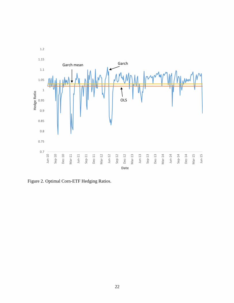
The optimal hedge ratios estimated using the different regression methods for each commodity
can be found in Table 5 along with the R-squared values of the models. Cointegration was not
found to be present between the ETF and cash price series for live cattle. Therefore an ECM
model was not used to find an optimal ETF hedge ratio for live cattle. The reported GARCH
ratio is the average of the time-varying ratios found using the GARCH model. The time-varying
ratios can be found in Figures 1- 8, along with the OLS and ECM estimates. These figures show
the results of all three regression models used along with the mean of the GARCH hedge ratios.
Futures hedge ratios and ETF hedge ratios were calculated over the same period of time for each
commodity. The main takeaway from these figures is to see how the optimal hedge ratio will
vary over time when using the GARCH model, and the OLS and ECM models are constant.
It was found that hedge ratios for futures and ETFs do not vary greatly across the different types
of models. For corn futures, the GARCH model returns a higher optimal hedge ratio, but for a
corn ETF hedge the OLS, ECM, and GARCH ratios are almost identical. The ECM and GARCH
models for soybeans futures and ETFs result in higher hedge ratios than the OLS model. For live
cattle, the GARCH model provides slightly greater hedge ratios than the OLS and ECM hedge
ratios. The hedge ratios for diesel fuel are nearly identical across all three models for futures. The
GARCH model returns a slightly high hedge ratio for ETFs than the OLS or ECM.
It was also found that an ETF hedge performs just as well as a futures hedge. For corn and
soybeans the ETF hedge ratio is higher that the futures hedge ratio for each model. A t-test of
14
OLS hedges also shows that the futures and ETF hedge ratios for corn and soybeans are
statistically different. The hedge ratios for corn and soybeans also show that futures and ETFs do
a good job covering a producer’s price risk with hedge ratios near one. The Corn ETF hedge
shows that a producer would want to hedge his total quantity.
The ETF hedge ratio for live cattle and diesel are nearly identical to the futures hedge ratio for
each model. Further, OLS hedges are not statistically different from each other. The futures and
ETF optimal hedge ratios for live cattle range from 0.45 to 0.50. The diesel futures and ETF
hedge ratios show that hedging using heating oil futures and ETFs perform rather poorly in
protecting a producer against price risk.
The reported R-square values can be used to judge how well each model predicts. The ETF OLS
model for corn has a higher R-squared value than the futures, but the ECM futures model has a
slightly higher R-squared than the ETF model. The soybeans futures OLS model R-squared is
higher than the ETF OLS model, while the ECM futures model is significantly higher than the
ETF ECM model. The live cattle futures model R-square is higher than then ETF, and the diesel
R-squared values are similar for both futures and ETFs.
The optimal hedging ratio for a risk adverse corn producer can be seen in figure 9. The
maximum certainty equivalent corresponds with a hedge ratio of 0.95 for futures and 0.85 for
ETFs. The optimal hedging ratio for futures from simulations is higher compared to the optimal
hedging ratios found using the regression techniques. The optimal ETF hedge ratio from
simulations is lower than the optimal ETF hedge ratio found using regression techniques. This
shows that in the presence of risk aversion the ETF hedge loses some effectiveness.
The optimal hedging ratio for futures from simulations is higher compared to the optimal
hedging ratios from regression techniques for soybeans. The optimal soybean hedge ratios for a
risk averse producer can be found in figure 10. It can be seen in this figure that the corresponding
optimal hedge ratio for the maximum certainty equivalent for a futures hedge is 0.975 and the
ETF hedge is 0.825. While the futures optimal hedge ratio is higher than the optimal hedge ratios
from the regression techniques, the ETF hedge ratio is again lower. This shows that an ETF
hedge of soybeans loses some effectiveness in the presence of risk aversion.
Figure 11 shows the optimal diesel hedge ratios for a moderately risk averse producer. It was
found that a slightly risk averse producer, or risk coefficient of 1, would not hedge diesel fuel
using futures or ETFs. Therefore the risk coefficient was increased to 2. Both an ETF and futures
hedge have near the same optimal hedge ratio at the maximum certainty equivalent. The optimal
diesel futures hedge ratio for a risk averse producer is slightly higher at 0.2 than the optimal ETF
hedge ratio at 0.175. The simulation optimal hedge ratios are both slightly higher than the
optimal hedge ratios found using the regression techniques.

15
Conclusion
This study has investigated the effectiveness of Exchange Traded Funds as a hedging tool. OLS,
ECM, and GARCH regression models were used to find optimal hedge ratios for corn, soybeans,
live cattle, and diesel fuel. Simulations were used to find the optimal hedge ratios for corn,
soybeans, and diesel fuel for a risk averse producer.
Based on regression results, an ETF hedge of corn and soybeans outperforms a futures hedge. A
reason for this outperformance can be that the corn and soybean ETFs incorporate more
information that is available in the futures market by being composed of multiple futures
contracts. On the other hand, hedging with futures only uses the information from a single
futures contract. The diesel ETF incorporates information from a single futures contract as it is
composed of only the nearby futures contract. This could account for the similar futures and ETF
hedging ratios in the case of diesel fuel.
Simulations show the opposite outcome though. Across all three commodities, the futures hedge
outperforms the ETF hedge. This highlights the effects of higher trading costs of ETFs as
compared to futures in the presence of risk aversion. These higher trading costs offset the
effectiveness gains of the ETF hedge.
An extension of this research would be to look at various locations. Mississippi is not a large
corn growing state, and it would be interesting to see if these results hold in the Corn Belt states
like Iowa and Illinois. There also exist ETFs for other commodities such as wheat, cotton and
sugar cane. On the input side, ETFs could possibly be used to hedge a producer’s fertilizer price
risk. Other ETFs exist that are stock based instead of futures based. These ETFs exist for various
commodities, and it would be interesting to see if they can be used to hedge as effectively as a
futures based ETF. A further extension of the simulation approach can be to see how varying
degrees of risk aversion effect the optimal hedge ratio.
This study has shown that ETFs have the potential to be used as an effective price risk
management tool just as futures contracts. The effectiveness of ETFs will provide small
producers a tool to manage their price risk in areas where they currently have no price risk
management tools.

16
References
Alexander, C., and A. Barbosa. 2007. “Effectiveness of Minimum-Variance Hedging.” The
Journal of Portfolio Management 33(2): 46-59.
Arias, J. B., W. Brorsen, and A. Harri. “Optimal Hedging Under Nonlinear Borrowing Cost,
Progressive Tax Rates, and Liquidity Constraints.” Journal of Futures Markets 20(4):
375-396
Baillie, R., and R. Myers. 1991 "Bivariate Garch Estimation of the Optimal Commodity Futures
Hedge." J. Appl. Econ. 6.2: 109-124.
Buguk, C., D. Hudson, and T. Hanson. 2003. “Price Volatility Spillover in Agricultural Markets:
An Examination of U.S. Catfish Markets.” Journal of Agricultural and Resource
Economics 28(1): 86-99.
Cecchetti, S. G., R. E. Cumby, and S. Figlewski. 1988. “Estimation of the Optimal Futures
Hedge.” Review of Economics and Statistics 70: 623-630.
Cheung,C.S., Kwan, C. C. Y., and Yip, P.C.Y. (1990). “The hedging Effectinvess of Options and
Futures: A mean-Gini Approach. Journal of Futures Markets 10: 61-74.
Chen, S., L. Cheng-few, and K. Shrestha. 2003. “Futures Hedge Ratios: A Review.” The
Quarterly Review of Economics and Finance 43(3): 433-465.
Collins, R. A. (1997). “Toward a Positive Economic Theory of Hedging.” American Journal of
Agricultural Economics 76(2): 488-499.
"Corn, Grain Sorghum & Wheat 2016 Planning Budgets." Budget Report No. 2015-03,
Department of Agricultural Economics, Mississippi State University, December 2015.
Ederington, L. 1979 "The Hedging Performance of the New Futures Markets." The Journal of
Finance 34(1): 157-170.
Elam, E. and J. Davis. 1990. “Hedging Risk For Feeder Cattle With a Traditional Hedge
Compared to a Ratio Hedge.” Southern Journal of Agricultural Economics 22:209-216.
Garbade, K. D., and W. L. Silber. 1983. “Price Movement and Price Discovery in Futures and
Cash Markets.” Review of Economics and Statistics 65: 289-297.
Ghosh. A. 1993. “Cointegration and Error Correction Models: Intertemporal Causality Between
Index and Futures Prices.” Journal of Futures Markets 13: 193-198.
Howard, C. T., and D’Antonio, L.J. (1984). “A risk-return measure of hedging effectiveness.”
Journal of Finacial and Quantitative Analysis 19: 101-112.

17
Harri, A. and D. Hudson. 2009. “Mean and Variance Dynamics between Agricultural
Commodity Prices and Crude Oil Prices and Implications for Hedging.” Presented at the
conference “Economics of Alternative Energy Sources & Globalization: The Road
Ahead”, Orlando, Florida, November 15-17.
Harri, A., L. Nalley, and D. Hudson. 2009. “The Relationship Between Oil, Exchange Rates,
and Commodity Prices.” Journal of Agricultural and Applied Economics 41(2):1-10.
Johnson, L. 1960. “The Theory of Hedging and Speculation in Commodity Futures.” The Review
of Economic Studies 139-151.
Kroner, K., and J. Sultan. 1993 "Time-varying distributions and dynamic hedging with foreign
currency futures." Journal of Financial and Quantitative Analysis 28(04): 535-551.
Lapan, H. and Moschini, G. 1994. “Futures Hedging Under Price, Basis, and Production Risk.”
American Journal of Agricultural Economics 76(3): 465-477.
Lien, D. 2004. “Cointegration and the Optimal Hedge Ratio: The General Case.” Quarterly
Review of Economics and Finnance 44: 654-658.
Lien, D., and Y. K. Tse. (1998). “Hedging Time-varying Downside Risk.” Journal of Futures
Markets 18: 705-722.
Lien, D., and Y. K. Tse. (2000). “Hedging Downside Risk with Futures Contracts.” Applied
Financial Economics 10: 163-170.
Mattos, F., P Garcia, and C. Nelson. 2008. “Relaxing Standard Hedging Assumptions in the
Presence of Downside Risk.” The Quarterly Review of Economics and Finance 48: 78-93.
Moschini, G. and R. Myers. 2002 “Testing for Constant Hedge Ratios in Commodity Markets: A
Multivariate Approach.” Journal of Empirical Finance 9: 589-603.
Murdock, M., and N. Richie. 2008 "The United States Oil Fund as a Hedging
Instrument." Journal of Asset Management 9(5): 333-346.
Myers, R., and S. Thompson. 1989. “Generalized Optimal Hedge Ratio Estimation.” American
Journal of Agricultural Economics 71: 858-868.
Plamondon, J., and C. Luft. 2012 "Commodity Exchange-Traded Funds: Observations on Risk
Exposure and Performance." Available at SSRN 2139711.
Schweikhardt, D. 2009. “Agriculture in a Turbulent Economy – A New Era of Instability?”
Choices 24(1): 4-5.
18
"Soybeans 2016 Planning Budgets." Budget Report No. 2015-02, Department of Agricultural
Economics, Mississippi State University, October 2015.
United States Department of Agriculture, 2014. “2012 Census of Agriculture: Mississippi State
and County Data.” AC-12-A-24.

19
Table 1. Summary Statistics of Corn Cash, Futures, and ETF prices (Levels and Log-Prices)
Variable Sample Mean (s.d.) Min Max
# of
obs Skewness Kurtosis
Cash Price 5.61(1.35) 3.06 7.83 263 -0.099 -1.412
Futures Price 5.58(1.45) 3.21 8.30 263 -0.026 -1.442
ETF Price 36.41(8.01) 22.63 52.50 263 -0.056 -1.148
Log Cash Price 1.69(0.25) 1.12 2.06 263 -0.326 -1.263
Log Futures Price 1.68(0.27) 1.17 2.12 263 -0.245 -1.414
Log ETF Price 3.57(0.23) 3.12 3.96 263 -0.333 -1.109
Notes: Cash Price - Greenville, Mississippi, ETF- Teucrium Corn Fund
Table 3. Summary Statistics of Live Cattle Cash, Futures, and ETF prices (Levels and Log-Prices)
Variable Sample Mean (s.d.) Min Max
# of
obs Skewness Kurtosis
Cash Price 113.86(24.16) 79.97 172.00 371 0.559 -0.600
Futures Price 113.74(2.12) 80.15 170.90 371 0.436 -0.677
ETF Price 31.35(2.16) 25.66 49.48 371 1.836 2.382
Log Cash Price 4.71(0.21) 4.38 5.15 371 0.244 -0.969
Log Futures Price 4.71(0.20) 4.38 5.14 371 0.131 -1.027
Log ETF Price 3.43(0.16) 3.24 3.90 371 1.591 1.641
Notes: Cash Price - Texas and Oklahoma, ETF- iPath Bloomberg Livestock Subindex Total
Return ETN
Table 2. Summary Statistics of Soybeans Cash, Futures, and ETF prices (Levels and Log-Prices)
Variable Sample Mean (s.d.) Min Max
# of
obs Skewness Kurtosis
Cash Price 13.24(2.09) 9.13 17.53 197 -0.209 -0.984
Futures Price 13.05(2.12) 9.17 17.63 197 -0.195 -0.832
ETF Price 23.01(2.16) 18.51 28.53 197 -0.004 -0.436
Log Cash Price 2.57(0.16) 2.21 2.86 197 -0.429 -0.971
Log Futures Price 2.55(0.17) 2.21 2.87 197 -0.450 -0.865
Log ETF Price 3.13(0.09) 2.92 3.35 197 -0.213 -0.523
Notes: Cash Price - Greenville, Mississippi, ETF- Teucrium Soybean Fund

20
Table 4. Summary Statistics of Diesel Cash, Futures, and ETF prices (Levels and Log-Prices)
Variable Sample Mean (s.d.) Min Max n Skewness Kurtosis
Cash Price 3.41(0.62) 1.97 4.74 348 -0.419 -0.840
Futures Price 2.56(0.61) 1.16 4.10 348 -0.306 -0.7651
ETF Price 31.23(8.19) 17.80 65.68 348 1.783 4.7995
Log Cash Price 1.01(0.20) 0.68 1.56 348 -0.700 -0.522
Log Futures Price 0.91(0.26) 0.15 1.41 348 -0.730 -0.336
Log ETF Price 3.41(0.24) 2.88 4.18 348 0.635 1.454
Notes: Cash Price - Greenville, Mississippi, ETF- Teucrium Soybean Fund
Table 5. Regression Estimates of Futures and ETF Hedge Ratios for Corn, Soybeans,
Live Cattle, and Diesel
Hedge Ratios (R-Squared)
OLS ECM GARCH
Corn
Futures 0.78*
(0.5878)
0.77*
(0.6355)
0.82
ETF 1.02*
(0.6101)
1.02*
(0.6274)
1.03
Soybeans
Futures 0.83*
(0.5756)
0.87*
(0.6889)
0.87
ETF 0.96*
(0.5126)
0.99*
(0.5319)
1.03
Live Cattle
Futures 0.47
(0.3141)
0.48
(0.5250)
0.50
ETF 0.45
(0.2606)
n/a 0.49
Diesel
Futures 0.15
(0.1806)
0.15
(0.7213)
0.16
ETF 0.15
(0.1746)
0.14
(0.6795)
0.17
Note: R-Squared values in parenthesis

21
Figure 1. Optimal Corn-Futures Hedging Ratios.
0
0.2
0.4
0.6
0.8
1
1.2
1.4Ju
n-1
0
Sep
-10
Dec
-10
Mar
-11
Jun
-11
Sep
-11
Dec
-11
Mar
-12
Jun
-12
Sep
-12
Dec
-12
Mar
-13
Jun
-13
Sep
-13
Dec
-13
Mar
-14
Jun
-14
Sep
-14
Dec
-14
Mar
-15
Jun
-15
He
dge
Rat
io
Date
Garch meanGarch
OLS
22
Figure 2. Optimal Corn-ETF Hedging Ratios.
0.7
0.75
0.8
0.85
0.9
0.95
1
1.05
1.1
1.15
1.2Ju
n-1
0
Sep
-10
Dec
-10
Mar
-11
Jun
-11
Sep
-11
Dec
-11
Mar
-12
Jun
-12
Sep
-12
Dec
-12
Mar
-13
Jun
-13
Sep
-13
Dec
-13
Mar
-14
Jun
-14
Sep
-14
Dec
-14
Mar
-15
Jun
-15
He
dge
Rat
io
Date
Garch mean Garch
OLS

23
Figure 3. Optimal Soybeans-Futures Hedging Ratios.
0.4
0.6
0.8
1
1.2
1.4
1.6
1.8
2
Oct
-11
Dec
-11
Feb
-12
Ap
r-1
2
Jun
-12
Au
g-1
2
Oct
-12
Dec
-12
Feb
-13
Ap
r-1
3
Jun
-13
Au
g-1
3
Oct
-13
Dec
-13
Feb
-14
Ap
r-1
4
Jun
-14
Au
g-1
4
Oct
-14
Dec
-14
Feb
-15
Ap
r-1
5
Jun
-15
He
dge
Rat
io
Date
Garch mean
Garch
OLS

24
Figure 4. Optimal Soybean-ETF Hedging Ratios.
0.5
0.6
0.7
0.8
0.9
1
1.1
1.2
1.3
1.4
Oct
-11
Dec
-11
Feb
-12
Ap
r-1
2
Jun
-12
Au
g-1
2
Oct
-12
Dec
-12
Feb
-13
Ap
r-1
3
Jun
-13
Au
g-1
3
Oct
-13
Dec
-13
Feb
-14
Ap
r-1
4
Jun
-14
Au
g-1
4
Oct
-14
Dec
-14
Feb
-15
Ap
r-1
5
Jun
-15
He
dge
Rat
io
Date
OLS
Garch
Garch Mean

25
Figure 5. Optimal Live Cattle-Futures Hedging Ratios.
0.3
0.4
0.5
0.6
0.7
0.8
0.9
1
No
v-0
7
Feb
-08
May
-08
Au
g-0
8
No
v-0
8
Feb
-09
May
-09
Au
g-0
9
No
v-0
9
Feb
-10
May
-10
Au
g-1
0
No
v-1
0
Feb
-11
May
-11
Au
g-1
1
No
v-1
1
Feb
-12
May
-12
Au
g-1
2
No
v-1
2
Feb
-13
May
-13
Au
g-1
3
No
v-1
3
Feb
-14
May
-14
Au
g-1
4
No
v-1
4
Feb
-15
He
dge
Rat
io
Date
Garch
Garch Mean
OLS

26
Figure 6. Optimal Live Cattle-ETF Hedging Ratios.
0.2
0.3
0.4
0.5
0.6
0.7
0.8
No
v-0
7
Feb
-08
May
-08
Au
g-0
8
No
v-0
8
Feb
-09
May
-09
Au
g-0
9
No
v-0
9
Feb
-10
May
-10
Au
g-1
0
No
v-1
0
Feb
-11
May
-11
Au
g-1
1
No
v-1
1
Feb
-12
May
-12
Au
g-1
2
No
v-1
2
Feb
-13
May
-13
Au
g-1
3
No
v-1
3
Feb
-14
May
-14
Au
g-1
4
No
v-1
4
Feb
-15
He
dge
Rat
io
Date
Garch
Garch Mean
OLS

27
Figure 7. Optimal Diesel-Futures Hedging Ratios.
0
0.05
0.1
0.15
0.2
0.25
0.3
Ap
r-0
8
Jul-
08
Oct
-08
Jan
-09
Ap
r-0
9
Jul-
09
Oct
-09
Jan
-10
Ap
r-1
0
Jul-
10
Oct
-10
Jan
-11
Ap
r-1
1
Jul-
11
Oct
-11
Jan
-12
Ap
r-1
2
Jul-
12
Oct
-12
Jan
-13
Ap
r-1
3
Jul-
13
Oct
-13
Jan
-14
Ap
r-1
4
Jul-
14
Oct
-14
Jan
-15
Ap
r-1
5
He
dge
Rat
io
Date
OLS
Garch Mean
Garch

28
Figure 8. Optimal Diesel-ETF Hedging Ratios.
0
0.05
0.1
0.15
0.2
0.25
0.3
0.35
Ap
r-0
8
Jul-
08
Oct
-08
Jan
-09
Ap
r-0
9
Jul-
09
Oct
-09
Jan
-10
Ap
r-1
0
Jul-
10
Oct
-10
Jan
-11
Ap
r-1
1
Jul-
11
Oct
-11
Jan
-12
Ap
r-1
2
Jul-
12
Oct
-12
Jan
-13
Ap
r-1
3
Jul-
13
Oct
-13
Jan
-14
Ap
r-1
4
Jul-
14
Oct
-14
Jan
-15
Ap
r-1
5
Jul-
15
He
dge
Rat
io
Date
Garch
Garch Mean
OLS

29
Figure 9. Corn Simulation Hedge Ratios
0
500
1000
1500
2000
2500
3000
3500
4000
0 0.1 0.2 0.3 0.4 0.5 0.6 0.7 0.8 0.9 1 1.1 1.2
Ce
rtai
nty
Eq
uiv
ale
nt
Hedge Ratio
Futures
ETF
Max = .95
Max = .85

30
Figure 10. Simulation Optimal Soybean Hedge Ratio
-2000
-1000
0
1000
2000
3000
4000
5000
6000
7000
0 0.1 0.2 0.3 0.4 0.5 0.6 0.7 0.8 0.9 1 1.1 1.2
Ce
rtai
nti
y Eq
uiv
ale
nt
Hedge Ratios
Futures
ETF
Max = .975
Max = .825

31
Figure 11. Diesel Simulation Optimal Hedge Ratios
0
50
100
150
200
250
300
350
400
0 0.1 0.2 0.3 0.4 0.5 0.6 0.7 0.8 0.9 1 1.1 1.2
Ce
rtai
nty
Eq
uiv
ale
nt
Hedge Ratio
Futures
ETF
Max = 0.2
Max = 0.175