by tenko raykov - scientific software international, inc. · by tenko raykov this document ......

Scale reliability evaluation 1

Scale Reliability Evaluation With LISREL 8.50 by Tenko Raykov

This document describes covariance structure analysis methods for estimation of scale

reliability and dealing with related issues, which can be used with LISREL8.50. The following discussion is focused on the reliability coefficient. This is a main

psychometric index reflecting "precision" (consistency) of measurement in the behavioral, educational and social sciences, which is defined as the overall (unconditional) percentage of true variance in observed variance on a given measure. The procedures outlined below accomplish goals of earlier methods based on Cronbach's coefficient alpha (α; Cronbach, 1951) in the setting of pre-specified scale components (tests, test parts) and sampling of subjects. As is well known, with uncorrelated errors (and regardless of factorial structure of the components) coefficient α equals scale reliability—the quantity of actual interest to scale constructors and developers—only in the very restrictive case when all elements of a multiple-component instrument are tau-equivalent, and otherwise underestimates it even at the population level (Novick & Lewis, 1967; Lord & Novick, 1968; Zimmerman, 1972). Tau-equivalence is a rather restrictive condition in these sciences where units of measurement are frequently arbitrary. (This testable condition requires that the measurement units are in addition equal to one another.) Alternatively, with correlated errors, α can overestimate or conversely underestimate scale reliability already in the population (e.g., Zimmerman, 1972; Raykov, 2001a, in press/2001b).

The major feature of the estimation and testing approaches in the sequel is that they allow one to answer a number of important questions in the same terms in which the questions are asked. This feature is not shared with many applications of α in relation to reliability. The present approaches permit one to (i) estimate scale reliability (not α); (ii) construct confidence interval for scale reliability (not α); (iii) test if scale reliability is the same in independent or dependent groups (not whether α is so); and (iv) examine if after revision, such as adding/deleting components, the new scale has the same reliability as the old one (not whether α for the new scale is the same as α for the old one) in the population for which the instrument is being developed (rather than only in the sample at hand, as is the case with currently typical applications of α for these purposes). Thus, the methods outlined in the remainder answer relevant and often raised queries in the behavioral and social sciences about reliability of multi-component measuring instruments and thereby provide their answers in terms of the ultimate index of concern, the scale reliability coefficient.

In this way, the methods described below fulfill a major logical prerequisite. Accordingly, if a question is asked in terms of concept(s) A say, then its answer ought to be given in terms of A, not in terms of another concept(s) (that only under potentially rather restrictive conditions equal A). That is, with the following procedures one answers questions about scale reliability and the answers are provided in terms of scale reliability, in which terms the questions were asked in the first instance. Traditional and currently still popular methods addressing these questions answer them in terms of α rather than scale reliability. Those methods obviously do not fulfill this fundamental logical requirement, due to the well-documented fact that α is in general a misestimator of scale reliability even if one had access to the entire population.

The research on which this document is based was supported by grants from Scientific Software International and The College Entrance and Examination Board (##2000-225, 2001-173, 2001-267), which are herewith gratefully acknowledged. I am also thankful to Drs. Patrick E. Shrout and David A. Grayson for stimulating discussions on some of the issues dealt with in the remainder (specifically, on multi-dimensional scale reliability estimation and testing for reliability change in a studied population as a result of scale revision). The detailed developments, discussions and rationale of the methods outlined below can be found in the papers and manuscripts in press that are cited in the reference section at the end of this document.


0. Notation and Background

This document assumes throughout that a scale(s) of interest is given a priori, i.e., its components (tests, sub-tests or test parts) are pre-specified (Lord, 1955). The subject population(s) under investigation is assumed to be well-defined and from it a random sample(s) of subjects drawn to whom the scale(s) is administered. The components of the scale are denoted Y1, Y2, ..., Yk. If they are congeneric (Joreskog, 1971),

(1) Yi = ai + biη + Ei hods true, where ai and bi are appropriate constants, η the common true score (e.g., η = T1 can be taken, with T1 being the true score of Y1), and Ei are the corresponding error scores (i = 1, 2, ..., k; for a definition of true and error scores, see Zimmerman, 1975). For identifiability, let Var(η) = 1, where Var(.) denotes variance in the population.

We will be concerned with various issues related directly to the reliability coefficient ρY of the total scale score Y = Y1 + Y2 + … + Yk , which is also refered to as "scale reliability" or "composite reliability". With uncorrelated errors this coefficient, defined as the ratio of true variance in Y to its observed variance (e.g., Lord & Novick, 1968), equals:

(2) ρY =

∑ ∑

∑

= =

=

+k

i

k

iiii

k

ii

b

b

1 1

2

1

2

)(

)(

θ ,

where θii = Var(Ei) are the error variances (i = 1, 2, ..., k, e.g., Bollen, 1989; numerators and denominators of reliability coefficients are assumed throughout distinct from zero, a typically fulfilled assumption in empirical research). With correlated errors (e.g., Williams & Zimmerman, 1996; Zimmerman, 1972),

(3) ρY =

∑ ∑ ∑

∑

= = <≤

=

++k

i

k

i kjiijiii

k

ii

b

b

1 1 1

2

1

2

2)(

)(

θθ≤

,

where θij (1≤i<j≤k) are the nonzero error covariances and i and j vary across all pairs of correlated errors. We presume that all models dealt with in the rest are identified. For a weighted scale Y = w1Y1 + w2Y2 + ... + wkYk , it follows that

(4) ρY =

∑ ∑

∑

= =

=

+k

i

k

iiiiii

k

iii

wbw

bw

1 1

22

1

2

)(

)(

θ

in the uncorrelated error case, and in that with correlated errors

(5) ρY =

∑ ∑ ∑

∑

= = ≤<≤

=

++k

i

k

i jjiijjiiiiii

k

iii

wwwbw

bw

1 1 1

22

1

2

2)(

)(

θθ,

where the same notation for the error covariances is used as in Equation (3). For the purposes of the remaining discussion, the weighted scale case is reducible to the unweighted case via appropriate substitutions (e.g., Raykov, in press/2001b).


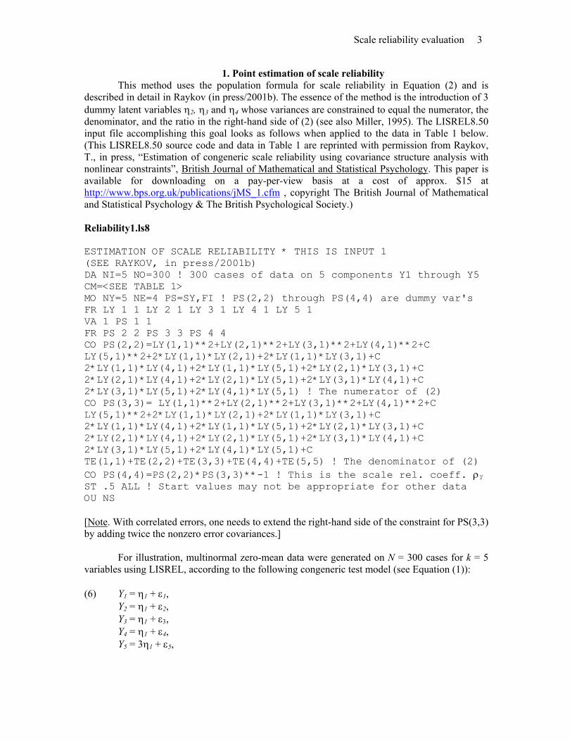
1. Point estimation of scale reliability This method uses the population formula for scale reliability in Equation (2) and is

described in detail in Raykov (in press/2001b). The essence of the method is the introduction of 3 dummy latent variables η2, η3 and η4 whose variances are constrained to equal the numerator, the denominator, and the ratio in the right-hand side of (2) (see also Miller, 1995). The LISREL8.50 input file accomplishing this goal looks as follows when applied to the data in Table 1 below. (This LISREL8.50 source code and data in Table 1 are reprinted with permission from Raykov, T., in press, “Estimation of congeneric scale reliability using covariance structure analysis with nonlinear constraints”, British Journal of Mathematical and Statistical Psychology. This paper is available for downloading on a pay-per-view basis at a cost of approx. $15 at http://www.bps.org.uk/publications/jMS_1.cfm , copyright The British Journal of Mathematical and Statistical Psychology & The British Psychological Society.) Reliability1.ls8 ESTIMATION OF SCALE RELIABILITY * THIS IS INPUT 1 (SEE RAYKOV, in press/2001b) DA NI=5 NO=300 ! 300 cases of data on 5 components Y1 through Y5 CM=<SEE TABLE 1> MO NY=5 NE=4 PS=SY,FI ! PS(2,2) through PS(4,4) are dummy var's FR LY 1 1 LY 2 1 LY 3 1 LY 4 1 LY 5 1 VA 1 PS 1 1 FR PS 2 2 PS 3 3 PS 4 4 CO PS(2,2)=LY(1,1)**2+LY(2,1)**2+LY(3,1)**2+LY(4,1)**2+C LY(5,1)**2+2*LY(1,1)*LY(2,1)+2*LY(1,1)*LY(3,1)+C 2*LY(1,1)*LY(4,1)+2*LY(1,1)*LY(5,1)+2*LY(2,1)*LY(3,1)+C 2*LY(2,1)*LY(4,1)+2*LY(2,1)*LY(5,1)+2*LY(3,1)*LY(4,1)+C 2*LY(3,1)*LY(5,1)+2*LY(4,1)*LY(5,1) ! The numerator of (2) CO PS(3,3)= LY(1,1)**2+LY(2,1)**2+LY(3,1)**2+LY(4,1)**2+C LY(5,1)**2+2*LY(1,1)*LY(2,1)+2*LY(1,1)*LY(3,1)+C 2*LY(1,1)*LY(4,1)+2*LY(1,1)*LY(5,1)+2*LY(2,1)*LY(3,1)+C 2*LY(2,1)*LY(4,1)+2*LY(2,1)*LY(5,1)+2*LY(3,1)*LY(4,1)+C 2*LY(3,1)*LY(5,1)+2*LY(4,1)*LY(5,1)+C TE(1,1)+TE(2,2)+TE(3,3)+TE(4,4)+TE(5,5) ! The denominator of (2) CO PS(4,4)=PS(2,2)*PS(3,3)**-1 ! This is the scale rel. coeff. ρY ST .5 ALL ! Start values may not be appropriate for other data OU NS [Note. With correlated errors, one needs to extend the right-hand side of the constraint for PS(3,3) by adding twice the nonzero error covariances.] For illustration, multinormal zero-mean data were generated on N = 300 cases for k = 5 variables using LISREL, according to the following congeneric test model (see Equation (1)): (6) Y1 = η1 + ε1,

Y2 = η1 + ε2, Y3 = η1 + ε3, Y4 = η1 + ε4, Y5 = 3η1 + ε5,

http://www.bps.org.uk/publications/jMS_1.cfm


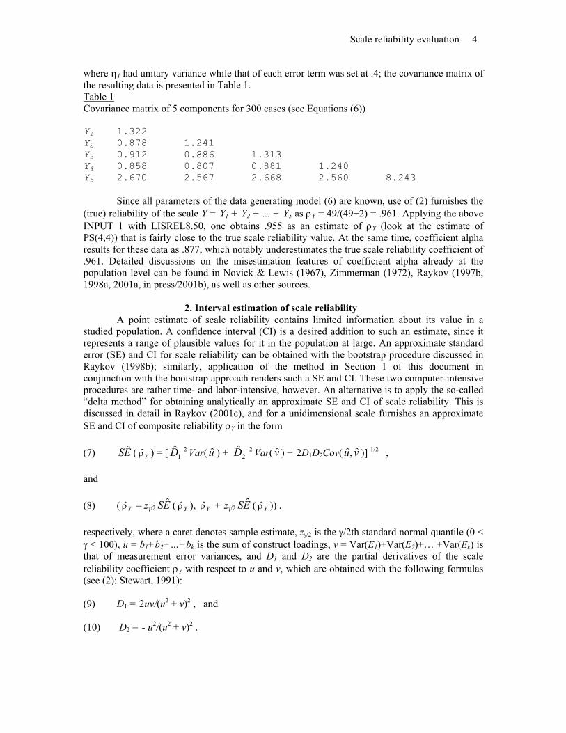
where η1 had unitary variance while that of each error term was set at .4; the covariance matrix of the resulting data is presented in Table 1. Table 1 Covariance matrix of 5 components for 300 cases (see Equations (6)) Y1 1.322 Y2 0.878 1.241 Y3 0.912 0.886 1.313 Y4 0.858 0.807 0.881 1.240 Y5 2.670 2.567 2.668 2.560 8.243 Since all parameters of the data generating model (6) are known, use of (2) furnishes the (true) reliability of the scale Y = Y1 + Y2 + ... + Y5 as ρY = 49/(49+2) = .961. Applying the above INPUT 1 with LISREL8.50, one obtains .955 as an estimate of ρY (look at the estimate of PS(4,4)) that is fairly close to the true scale reliability value. At the same time, coefficient alpha results for these data as .877, which notably underestimates the true scale reliability coefficient of .961. Detailed discussions on the misestimation features of coefficient alpha already at the population level can be found in Novick & Lewis (1967), Zimmerman (1972), Raykov (1997b, 1998a, 2001a, in press/2001b), as well as other sources.

2. Interval estimation of scale reliability A point estimate of scale reliability contains limited information about its value in a

studied population. A confidence interval (CI) is a desired addition to such an estimate, since it represents a range of plausible values for it in the population at large. An approximate standard error (SE) and CI for scale reliability can be obtained with the bootstrap procedure discussed in Raykov (1998b); similarly, application of the method in Section 1 of this document in conjunction with the bootstrap approach renders such a SE and CI. These two computer-intensive procedures are rather time- and labor-intensive, however. An alternative is to apply the so-called “delta method” for obtaining analytically an approximate SE and CI of scale reliability. This is discussed in detail in Raykov (2001c), and for a unidimensional scale furnishes an approximate SE and CI of composite reliability ρY in the form (7) ( ) = [ES ˆ

Yρ 1D 2 Var( ) + u 2D

2 Var( ) + 2Dv 1D2Cov( )] vu ˆ,ˆ 1/2 , and (8) ( – zYρ γ/2 ES ˆ ( ), + zYρ Yρ γ/2 ES ˆ ( )) , Yρ respectively, where a caret denotes sample estimate, zγ/2 is the γ/2th standard normal quantile (0 < γ < 100), u = b1+b2+…+bk is the sum of construct loadings, v = Var(E1)+Var(E2)+… +Var(Ek) is that of measurement error variances, and D1 and D2 are the partial derivatives of the scale reliability coefficient ρY with respect to u and v, which are obtained with the following formulas (see (2); Stewart, 1991): (9) D1 = 2uv/(u2 + v)2 , and (10) D2 = - u2/(u2 + v)2 .


The estimates of D1 and D2 are furnished by substitution into (9) and (10) of the estimates of u and v yielded by the following LISREL8.50 input file (STEP 1). The variances and covariance of the estimates of u and v are found as pertinent entries in the matrix of COVARIANCES OF PARAMETER ESTIMATES in the LISREL output obtained thereby. Then, to get an approximate SE and CI of scale reliability, a few simple computations are performed with a major statistical software, e.g., SPSS (STEP 2 input file; the LISREL8.50 and following SPSS input files as well as data in Table 2 are reprinted with permission from Raykov, T. 2001c, “Analytic estimation of standard error and confidence interval for scale reliability”. Multivariate Behavioral Research, in press). Reliability2.ls8 ESTIMATION OF STANDARD ERROR OF SCALE RELIABILITY (STEP 1) THIS IS INPUT 2 DA NI=5 NO=500 ! Sample size for data in Table 2 CM=<SEE TABLE 2> MO NY=5 NE=3 PS=DI,FI ! Need PS(2,2) AND PS(3,3)as dummy param. VA 1 PS(1,1) ! Latent variance set at 1, for identifiability FR LY 1 1 LY 2 1 LY 3 1 LY 4 1 LY 5 1 CO PS(2,2)=LY(1,1)+LY(2,1)+LY(3,1)+LY(4,1)+LY(5,1) ! This is u CO PS(3,3)=TE(1,1)+TE(2,2)+TE(3,3)+TE(4,4)+TE(5,5) ! This is v OU ALL ND=3 ! ‘ALL’ yields the parameter estimates’ cov. matrix

[Note. The variances and covariance of the estimates of the parametric expressions u (PSI(2,2)) and v (PSI(3,3)) are located as pertinent entries of the output section “Covariance matrix of parameter estimates”. Alternatively, the variances of the estimates of u and v are their squared standard errors reported by LISREL in the “LISREL estimates” section.] TITLE ‘SPSS INPUT FOR SE AND CI OF SCALE RELIABILITY (STEP 2)’. COMP U=9.941. COMP V=3.892. COMP D1=2*U*V/(U**2+V)**2. COMP D2= -U**2/(U**2+V)**2. COMP VAR_U=.107. COMP VAR_V=.019. COMP COV_UV= -.001. COMP SR=U**2/(U**2+V). COMP SE = SQRT(D1**2*VAR_U+D2**2*VAR_V+2*D1*D2*COV_UV). COMP CI90_LO=SR-1.645*SE. COMP CI90_UP=SR+1.645*SE. EXECUTE. [Note. CI = confidence interval; SR = scale reliability coefficient (ρY); U, V = u and v in Equations (7) through (10); D1 and D2 = estimates of the derivatives of scale reliability with respect to u and v (see (9) and (10)); SE = estimate of standard error of the scale reliability coefficient; VAR_U, VAR_V, COV_UV = variances and covariance of the estimates of u and v; CI90_LO, CI90_UP = lower and upper endpoint of the (approximate) 90%-CI for scale reliability. The numbers entered above in this SPSS input equal these estimates for the following example. In the last 2 lines, change correspondingly the standard normal quantiles if another confidence level is of concern.]


For illustration, this two-step interval estimation procedure is applied on simulated data (cf. Raykov, 2001c). Using LISREL, miltinormal zero-mean data were generated on k = 5 variables for N = 500 cases, following the model

(11) Y1 = T1 + E1 ,

Y2 = 1.5T1 + E2 , Y3 = 2T1 + E3 , Y4 = 2.5T1 + E4 , Y5 = 3T1 + E5 ,

whereby the latent score T1 was simulated with variance 1, and the error variances generated at .4, .6, .8, 1, and 1.2 for E1 to E5, respectively. The covariance matrix of the so-obtained data on Y1 through Y5 is presented in Table 2.

Table 2 Covariance matrix of 5 variables for 500 cases (see Equations (11)) Y1 1.384 Y2 1.484 2.756 Y3 1.988 2.874 4.845 Y4 2.429 3.588 4.894 6.951 Y5 3.031 4.390 6.080 7.476 10.313

Applying the above INPUT 2 with LISREL8.50 (STEP 1 input file) furnishes .962 as an estimate of the reliability coefficient of the scale Y = Y1 + Y2 + … + Yk. Since all population parameters are known, the (true) reliability of this scale is determined by substituting their values into (2): ρY = (1+1.5+2+2.5+3)2/[(1+1.5+2+2.5+3)2 +.4+.6+.8+1+1.2] = .962. By comparison, α = .931 results for this data set, which notably underestimates the true scale reliability of .962 and is similarly lower than its estimate rendered by the described approach (see also Raykov, 1997b). To obtain an approximate SE and 90%-CI for scale reliability, use the above SPSS file (STEP2 input file). To this end, u and are first found as the corresponding variances of ηˆ v 2 and η3 in the LISREL output: 9.941 and 3.892. With them, D1 and D2 are obtained from (9) and (10) as .007 and -.009, respectively. Then the variances and covariance of u and are located in the LISREL output section titled “Covariances of parameter estimates” correspondingly as .107, .019, and

ˆ v

-.001. With all these quantities, that SPSS file yields a standard error of .003 and a 90%-confidence interval for the scale reliability coefficient as (.958; .967), which covers the true scale reliability of .962. (Note that coefficient alpha in this data is outside the last CI.)

3. Point and interval estimation of noncongeneric scale reliability A number of potentially quite important substantive reasons, primarily validity related,

can lead behavioral, educational or social scientists to consider at times also noncongeneric (nonhomogeneous) scales. This section discusses how LISREL8.50 can be used to point- and interval estimate the reliability of such a scale, following the rationale and idea underlying the "omega" coefficient by McDonald (1985, 1999); details can be found in Raykov & Shrout (2002). Assume that k > 2 fixed measures Y1, Y2, ..., Yk are administered to a sample from a specified subject population, and that the reliability coefficient of their sum Y = Y1 + Y2 + ... + Yk is of concern (generalization to weighted scales is carried out directly along the following lines). We do not assume that Y1, Y2, ..., Yk are necessarily congeneric, i.e., it is possible that (a) more than a single trait be assessed by these k measures, and (b) some measures assess (load on) more


than one trait. Suppose that subsets of Y1, Y2, ..., Yk, if considered separately from the remaining items, assess common traits with unrestricted relationships. Thus, the initial set Y1, Y2, ..., Yk can be split into q subsets of items (1 ≤ q ≤ k), which subsets correspond to q constructs η1, η2, ..., ηq. We do not limit the number of items measuring any of the traits, and do not restrict the number of traits evaluated by any of the items, as long as the overall model dealt with next is identified. Without loss of generality, assume that the measures are ordered so that the q traits correspond to consecutive (not necessarily non-overlapping) subsets of Y1, Y2, ..., Yk: the first m1 of these k measures assess η1, the next m2 evaluate η2, ..., and the last mq components assess ηq (m1 + m2 + ... + mq = k; 1 ≤ mi ≤ k, i = 1, ..., q). The components within the jth of these subsets measure the same pertinent construct, ηj , with possibly different units of measurement and/or precision (i.e., are congeneric; Joreskog, 1971), and some components may also assess another trait(s) besides ηj (j = 1, …, q). Finally, for identifiability reasons, assume that all q latent constructs have variances of one, i.e., Var(ηi) = 1 (i = 1, …, q). This general setup contains as a special case that of congeneric measures, for q = 1. An example is given in the following Figure 1 (see also Equation (12) below) that represents the path diagram of the model fitted next (Raykov & Shrout, 2002). Following the rationale and idea of the "omega" coefficient by McDonald (1985, 1999), the reliability coefficient of the sum score Y for the model in Figure 1 can be obtained using covariance structure modeling (and application of the bootstrap subsequently yields an approximate SE and CI of reliability of Y; e.g., Raykov & Shrout, 2002, and below.) To demonstrate, we employ a simulated data set of multinormal zero-mean data generated on N = 300 cases for k = 6 components Y1 to Y6 using LISREL according to the model (12) Y1 = .5η1 + ε1 , Y2 = .8η1 + ε2 , Y3 = .6η1 + .3η2 + ε3 , Y4 = .4η1 + .4η2 + ε4 , Y5 = .5η2 + ε5 ,

Y6 = .8η2 + ε6 , where η1 and η2 evaluated by the battery of 6 components were simulated to have unitary variances and correlation Corr(η1,η2) = .3, and the error standard deviations were set at .7, .6, .6, .6, .7, and .6 for ε1 through ε6, respectively. The covariance matrix of Y1 through Y6 is presented in Table 3 (Raykov & Shrout, 2002b). Table 3 Covariance matrix of the six simulated variables (N = 300; see Equations (12)) Y1 0.58 Y2 0.32 0.95 Y3 0.31 0.48 0.83 Y4 0.23 0.37 0.41 0.72 Y5 0.01 0.05 0.19 0.24 0.78 Y6 0.09 0.21 0.36 0.36 0.43 0.93 The reliability coefficient of the scale score Y = Y1 + Y2 + ... + Yk is obtained with the LISREL8.50 input file provided next, which uses only linear parameter constraints and corresponds to the model in Figure 2 (that is the same as the model in Figure 1, with the added dummy variables for composite score Y, η3, and its true score, η4; the ratio of their variances is the reliability coefficient of Y--see Raykov & Shrout, 2002, and Equation (13) below. The LISREL 8.50 file, data in Table 3, and Figures 1 and 2 are reprinted with permission from


Raykov, T., Shrout, P., 2002, “Reliability of scales with general structure: Point and interval estimation using covariance structure modeling”, Structural Equation Modeling, in press). Reliability3.ls8 ESTIMATING RELIABILITY OF A COMPOSITE WITH GENERAL STRUCTURE [the added auxiliary variables Eta3 through Eta8, in the standard LISREL notation, stand for the error-purged scores (true scores) of Y1 to Y6; e.g., Raykov, 1997a] THIS IS INPUT 3 DA NI=6 NO=300 CM=<see Table 3> MO NY=6 NE=10 PS=SY,FI TE=ZE BE=FU,FI LE CONSTRC1 CONSTRC2 TRUE_Y1 TRUE_Y2 TRUE_Y3 TRUE_Y4 TRUE_Y5 C TRUE_Y6 COMPOSIT TRUE_CS ! TRUE_CS = TRUE SCORE OF Y, ! COMPOSIT = Y VA 1 PS 1 1 PS 2 2 FR BE 3 1 BE 4 1 BE 5 1 BE 6 1 ! These are the lambda’s for Eta1 FR BE 5 2 BE 6 2 BE 7 2 BE 8 2 ! These are the lambda’s for Eta2 FR PS 2 1 ! This is the latent construct's correlation VA 1 LY 1 3 LY 2 4 LY 3 5 LY 4 6 LY 5 7 LY 6 8 VA 1 BE 9 3 BE 9 4 BE 9 5 BE 9 6 BE 9 7 BE 9 8 ! This helps ! get Y (see Raykov, 1997a, Figure 1) FR PS 3 3 PS 4 4 PS 5 5 PS 6 6 PS 7 7 PS 8 8 ! These play the ! roles of the error var's FR BE 10 1 BE 10 2 ! Preparation for equality constraints next CO BE(10,1)=BE(3,1)+BE(4,1)+BE(5,1)+BE(6,1) ! These are the added CO BE(10,2)=BE(5,2)+BE(6,2)+BE(7,2)+BE(8,2) ! constraints, to get ! the composite Y and its true score ST .5 ALL OU NS AD=OFF ! Need last, as the matrix Ψ is not positive definite ! by construction [Note. Start values are valid for the used data set and may not be appropriate for others. To obtain a bootstrap standard error, analyzing the raw data produce with PRELIS B (≥200) resample covariance matrices; then analyze them with this LISREL input including as last the keywords BE=BEB PS=PSB; and finally study the distribution of the ratio of the variances of η4 to η3. This ratio is computed on the pertinent elements of the last two output files (viz. the 91st and 92nd columns of BEB and the 2nd, 6th, 10th, 15th, 21st, 28th, and 36th columns of PSB); see below.]

Applying INPUT 3 with LISREL8.50 we fit to the covariance matrix in Table 3 the two-factor model in Figure 2 with free factor loadings following the pattern in Equations (12), as well as free error variances and latent correlation; further, all paths leading from the observed variables into η4 are fixed at 1 to allow its interpretation as the scale score Y (see Raykov, 1997a; Raykov & Shrout, 2002). This yields acceptable goodness of fit indices: χ2 = 9.02, df = 6, p = .17 and RMSEA = .04 (0, .09). The estimate of the true composite variance (i.e., of η4) is found to be 10.83, while that of Y (i.e., of η3) turns out to be 13.09. Then the estimate of the reliability coefficient of the composite Y = Y1 + Y2 + ... + Y6 results as:


(13) = 10.83/13.09 = .83 . Yρ

Since in this example all parameters are known, the (true) reliability of Y is determined as: (14) ρY = Var[(.5+.8+.6+.4)η1 + (.3+.4+.5+.8)η2] /

{Var[(.5+.8+.6+.4)η1 + (.3+.4+.5+.8)η2] +.49+.36+.36+.36+.49+.36} = (2.32 + 22 + 2 x 2.3 x 2 x .3)/[(2.32 + 22 + 2 x 2.3 x 2 x .3) + 2.42] = .83 ,

which is the same as its estimate in (13) found with the discussed method but markedly underestimated by coefficient α that in this data set turns out to be .76 (see Raykov & Shrout, 2002). Next, resampling B = 1000 times from the original raw data set and fitting the model to each so-obtained sample furnishes 1000 bootstrap estimates of composite reliability. (Out of the 1000 model runs, 10 were associated with lack of convergence and were therefore disregarded in the following analyses.) The mean of these estimates is .84 and their standard deviation is .02. Hence, using the bootstrap approach (Efron & Tibshiriani, 1993), an approximate standard error of reliability of Y = Y1 + Y2 + … + Y6 results as SE( ) = .02. The 5Yρ th and 95th percentiles of the distribution of so-obtained resample composite reliability coefficients are thereby found to be .81 and .87, respectively. Using a simple approach to confidence interval construction, the last two numbers can be taken as a lower and upper limit of a bootstrap 90%-confidence interval for ρY , viz. (.81, .87). (We note that other, more involved methods of bootstrap-based CI construction can be used for this purpose as well; Efron & Tibshiriani, 1993.) This interval covers the true composite reliability of .83 (see Equation (14)) and is completely above .80 that may be considered a recommendable benchmark for reliability of scales. We stress that the estimated α of .76 in this data is markedly below both the point and interval estimates of composite reliability obtained with the method of this section, and also markedly below the true scale reliability coefficient (cf. Novick & Lewis, 1967).

Figure 1 (Raykov & Shrout, 2002)

η2 η1

ε1

Y1 Y2 Y3 Y4 Y5

ε6

Y6

ε2 ε3 ε4 ε5


Figure 2 (Raykov & Shrout, 2002)

Y1

ε1

Y2

ε2

Y3

ε3

Y4

ε4

Y5

ε5

η1 η2

λ11+λ21+λ32+λ41 λ32+λ42+λ52+λ62

1 1

1 1 1

1

η3

η4

ε6

Y6


4. Testing for differences in scale reliability across groups The question whether reliability of a scale is the same in two or more groups is frequently

of interest in behavioral, educational and social research. For example, it is of importance when examining whether some ethnic or gender groups may be disadvantaged at school when tested with an achievement or entrance examination test, in the sense of being associated with lower reliability on a multiple-item test. A number of examples can be also found in other social science discipliness, e.g., mental health research, where this question is similarly of interest.

To show how LISREL8.50 can be used to answer this question, assume that a multi-component instrument (scale) under consideration is given apriori, i.e., the set of its components is fixed (Lord, 1955), while the distinct populations (groups) of interest are prespecified and from them random samples of subjects are drawn to whom the scale(s) is administered. For any considered composite, suppose its components are congeneric (Joreskog, 1971). The details of the following procedure for testing group differences in reliability are contained in Raykov (in press/2002; full citation and information on accessibility is given below and in the References section). We are interested in testing the following null hypothesis with two groups: (15) Ho: ρ1Y = ρ2Y where the 1st subindex denotes group. To this end, we reparameterize the congeneric test model in the above Equation (1) by fixing the paths from the error terms into the observed variables to equal the sum of all construct loadings, i.e., b1 + b2 + ... + bk, within each group (k > 2; note that this does not change the identification status of the model.) To see how the null hypothesis (15) is equivalently transformed thereby, first denote the error term variances in each group by θr,ii (r = 1, 2, i = 1, ..., k), where the 1st subindex pertains to group. Symbolize then the squared sums of

construct loadings in the groups by B1 and B2 (i.e., B1 = ( and B∑=

k

iib

1

21 ) 2 = , where the

1

∑=

k

iib

1

22 )(

st subindex of the b's stands for group). Now, for the sake of (15), equate the reciprocals of the right-hand side of (2) for each group to one another, and observe after simple algebra that then (15) becomes equivalent to the cross-group constraint

(16) 2

,2

2

22,2

1 1

,1

2

11,2 ...BBBB

kkk

i

ii θθθθ−−−= ∑

=

in the uncorrelated error case, and in the correlated error case to

(17) ∑∑∑≤<≤≤<≤=

−−−−+=kji

ijkk

kji

ijk

i

ii

BBBBBB 1 2

,2

2

,2

2

22,2

1 1

,1

1 1

,1

2

11,2 2...2θθθθθθ

,

where θr,ij denote nonzero error covariances in the pertinent group. With the above mentioned reparameterization (viz. within each group set all paths from error terms into observed variables to equal the sum of their loadings on the latent variable), (16) and (17) are correspondingly equivalent to

(18) *θ ∑=

−−−=k

ikkii

1,222,2,111,2 *...** θθθ


and

(19) , ∑∑ ∑≤<≤= ≤<≤

−−−−+=kji

ij

k

ikk

kjiijii

1,2

1,222,2

1,1,111,2 *2*...**2** θθθθθθ

where each starred parameter stands for its corresponding ratio in (16) and (17), respectively. (Note that the starred parameters are the error variances and covariances, if any, of the reparameterized model.) Equations (18) and (19) represent each a cross-group linear constraint in terms of the rescaled error variances and covariances.

This procedure is next demonstrated with LISREL8.50 on the following numerical example. Multinormal, zero-mean data are first generated on m = 5 variables for N = 300 subjects in each of two groups. The two unrelated data sets are simulated using LISREL according to the following congeneric component models (this example and data is reprinted with permission from Raykov, T., in press/2002, “Examining group differences in reliability of multiple-component instruments”, British Journal for Mathematical and Statistical Psychology. This paper is available for downloading on a pay-per-view basis at a cost of approx. $15 at http://www.bps.org.uk/publications/jMS_1.cfm , copyright The British Journal of Mathematical and Statistical Psychology & The British Psychological Society.) In Group 1, the underlying model is (cf. Equation (1)): (20) Y1 = η1 + E1 ,

Y2 = 1.1η1 + E2 , Y3 = 1.2η1 + E3 , Y4 = 1.3η1 + E4 , Y5 = 1.4η1 + E5 ,

where the common true score η1 is generated as a standard normal variate while the variances of E1 to E5 are set at .8 and the covariance of E1 and E2 fixed at .6. In Group 2, the same model is employed with the only difference that the covariance of E1 and E2 is set at -.6; that is, the data generation model is defined here as: (21) Y1 = η1 + E1 ,

Y2 = 1.1η1 + E2 , Y3 = 1.2η1 + E3 , Y4 = 1.3η1 + E4 , Y5 = 1.4η1 + E5 ,

where the common true score η1 is a standard normal variate while the variances of E1 to E5 are set at .8 and the covariance of E1 and E2 fixed at -.6. The covariance matrices of the resulting data sets are presented in Table 4.



Table 4 Covariance matrices of the simulated two group data sets (see Equations (20) and (21)) ________________________________________________________________________ Component Y1 Y2 Y3 Y4 Y5 ________________________________________________________________________ Group 1 (N = 300) ________________________________________________________________________ Y1 1.602 Y2 1.580 1.982 Y3 1.071 1.299 2.260 Y4 1.168 1.353 1.474 2.287 Y5 1.308 1.489 1.750 1.661 2.783 ________________________________________________________________________ Group 2 (N = 300) ________________________________________________________________________ Y1 1.602 Y2 0.597 2.165 Y3 1.123 1.525 2.372 Y4 1.230 1.518 1.569 2.393 Y5 1.373 1.633 1.824 1.744 2.826 ________________________________________________________________________

To examine the relationship between the group reliability coefficients of the scale Y = Y1 + Y2 + ... + Y5 , first the reliability of Y is estimated in each group using the approach in Section 1 of this document. In Group 1, = .858 is obtained; since all parameters of the model used to generate the data are known, the (true) composite reliability coefficient is determined using Equation (2) as = 36/(36+4+1.2) = .874. In Group 2, = .923 is found, while the (true) scale reliability coefficient is similarly found via (2) as = 36/(36+4-1.2) = .928. Thus, by data generation the true group difference in scale reliability is notable, ∆ρ

Y,1ρ

Y,1ρ Y,2ρ

Y,2ρ

Y = ρ1,Y - ρ2,Y = .874 - .928 = -.054. To apply the outlined procedure with LISREL8.50, the following input file is used (reprinted with permission from Raykov, T., in press/2002, “Examining group differences in reliability of multiple-component instruments”, British Journal for Mathematical and Statistical Psychology; information on accessibility given above and in the References section): Reliability4.ls8 TESTING GROUP IDENTITY IN SCALE RELIABILITY * GROUP 1 THIS INPUT FILE IMPLEMENTS THE GROUP RELIABILITY EQUALITY CONSTRAINT (19) AFTER APPROPRIATELY RE-SCALING THE ERROR VARIANCES IN BOTH GROUPS (SEE (17) THIS IS INPUT 4 DA NO=300 NI=5 NG=2 CM=<see Table 4, Group 1> MO NY=5 NE=6 PS=SY,FI TE=ZE ! NEED PS(2,2) TO PS(6,6) FOR ! ERROR VARIANCES NEXT VA 1 PS 1 1 ! TRUE SCORE VARIANCE, SET TO 1 FOR IDENTIFIABILITY FR PS 2 2 PS 3 3 PS 4 4 PS 5 5 PS 6 6 PS 3 2 ! THESE BECOME ! NEXT THE RESCALED ERROR VARIANCES NEEDED BELOW FR LY 1 1 LY 2 1 LY 3 1 LY 4 1 LY 5 1 ! FREE CONSTRUCT LOADINGS


FR LY 1 2 LY 2 3 LY 3 4 LY 4 5 LY 5 6 ! PATHS FROM ERRORS TO ! OBSERVED VARIABLES; NEXT COME THE RESCALING CONSTRAINTS CO LY(1,2)=LY(1,1)+LY(2,1)+LY(3,1)+LY(4,1)+LY(5,1) CO LY(2,3)=LY(1,1)+LY(2,1)+LY(3,1)+LY(4,1)+LY(5,1) CO LY(3,4)=LY(1,1)+LY(2,1)+LY(3,1)+LY(4,1)+LY(5,1) CO LY(4,5)=LY(1,1)+LY(2,1)+LY(3,1)+LY(4,1)+LY(5,1) CO LY(5,6)=LY(1,1)+LY(2,1)+LY(3,1)+LY(4,1)+LY(5,1) ST .01 LY 1 1 LY 2 1 LY 3 1 LY 4 1 LY 5 1 ! THESE START ! VALUES MAY BE INAPPROPRIATE FOR OTHER DATA SETS ST .8 PS 3 3 PS 4 4 PS 5 5 PS 6 6 OU NS AD=OFF * GROUP 2 DA NO=300 NI=5 CM=<see Table 1, Group 2> MO NY=5 NE=6 PS=SY LY=SY,FI TE=ZE ! same pattern as in group 1 VA 1 PS 1 1 FR PS 2 2 PS 3 3 PS 4 4 PS 5 5 PS 6 6 PS 3 2 FR LY 1 1 LY 2 1 LY 3 1 LY 4 1 LY 5 1 FR LY 1 2 LY 2 3 LY 3 4 LY 4 5 LY 5 6 CO LY(1,2)=LY(1,1)+LY(2,1)+LY(3,1)+LY(4,1)+LY(5,1) CO LY(2,3)=LY(1,1)+LY(2,1)+LY(3,1)+LY(4,1)+LY(5,1) CO LY(3,4)=LY(1,1)+LY(2,1)+LY(3,1)+LY(4,1)+LY(5,1) CO LY(4,5)=LY(1,1)+LY(2,1)+LY(3,1)+LY(4,1)+LY(5,1) CO LY(5,6)=LY(1,1)+LY(2,1)+LY(3,1)+LY(4,1)+LY(5,1) CO PS(2,2)=PS(1,2,2)+PS(1,3,3)+PS(1,4,4)+PS(1,5,5)+PS(1,6,6)+C 2*PS(1,3,2)-PS(3,3)-PS(4,4)-PS(5,5)-PS(6,6)-2*PS(3,2) ST .9 LY 1 1 ST .01 LY 2 1 LY 3 1 ly 1 1 ly 4 1 ly 5 1 ! this is the critical constraint (19) for k=5 indicators and a ! pair of correlated errors. OU NS AD=OFF To test the null hypothesis (15), we fit two nested models--one without the restriction equivalent to (15) and the other with it (e.g., Joreskog & Sorbom, 1996); the difference in chi-square values of both models represents a test statistic of the hypothesis. The two-group congeneric test model (with related errors E1 and E2) having no group constraints is associated with a χ2 = 13.190, df = 8, p = .105, and RMSEA = .045 (0; .089), all indicating acceptable fit. The restricted model is obtained from the full by introducing (19) for k = 5 and a single pair of correlated errors (see the last constraint line of the LISREL input file.) This model is associated with χ2 = 33.150, df = 9, p = .0, and RMSEA = .093 (.060; .130), indicating lack of fit. The difference in chi-square values between the two models is ∆χ2 = 33.150 – 13.190 = 19.960, for difference in degrees of freedom being 1 and associated p < .001. This suggests rejection of Ho of equal reliability of Y = Y1 + Y2 + ... + Y5 in the two groups, in favor of the alternative of their difference. This conclusion is in agreement with the notable difference in the true scale reliability coefficients determined above, ∆ρY = -.054. In contrast, an application of the traditional procedure for studying scale reliability differences via comparison of alpha coefficients across groups would yield an incorrect conclusion. Indeed, the corresponding two-sample test (Feldt, 1969; see also Charter & Feldt 1996; Feldt, 1965; Feldt et al., 1987; Feldt & Ankenmann, 1998) is based on the statistic W = (1-αmin)/(1-αmax), where αmin is the


smaller and αmax the larger alpha coefficient in the groups. In the Group 1 data set, α = .902 is found, while in Group 2 α = .892 results. Hence W = .108/.098 = 1.102. [Note that coefficient alpha noticeably overestimates composite reliability in Group 1 and underestimates that reliability in Group 2 (e.g., Raykov, 2001a, in press/2001b).] Since W follows an F-distribution with degrees of freedom df

)1(ˆ

)2(ˆ

1 = df2 = 300 – 1 = 299 (e.g., Feldt, 1969), the associated probability value is p > .10 (obtained, e.g., via use of the SAS function PROBF(.,.,.); SAS Institute, 1988). Therefore, with this conventional method it would be incorrectly concluded that the null hypothesis (15) could not be rejected. This conclusion would contradict the notable difference in the true scale reliability coefficients, ∆ρYY = -.054, determined earlier and also sensed with the method outlined in this section. The incorrect end result with the conventional two-sample test would be explained with the misestimation of scale reliability by α in opposite directions in the two groups (e.g., Williams & Zimmerman, 1996; Zimmerman, 1972; Zimmerman et al., 1993; Raykov, 1997b, 2001a). In conclusion of this section, we note that in exactly the same manner one can test differences across groups in reliability of different scales (or different modes of administration/presentation of the same scale—e.g., paper-and-pensil vs. computer administration), or of the same scale across repeated assessments (Raykov, 2001d; see also Raykov, 2000). Similarly, the presented method is readily applied in settings with more than 2 groups (more than 2 repeated assessments), by imposing the critical constraint (18), or (19) if pertinent, on all subsequent pairs of groups or pairs of repeated assessments.

5. Testing for change in composite reliability as a result of scale development Examination if a revised scale, e.g., that obtained through addition or deletion of

components of an earlier scale, has higher reliability in a population of interest is essential if the modified composite is to be recommended for further use. Unfortunately, many scale construction and development researchers in the social sciences are currently preoccupied with comparing only the sample values of coefficient α before and after the revision took place. This practice is potentially seriously misleading on two counts. One, as indicated earlier, coefficient alpha cannot be considered a dependable estimator of scale reliability since already at the population level α misestimates the latter (Novick & Lord, 1967; Zimmerman, 1972; Raykov, 1997b, 1998a, 2001a, in press/2001b). Two, a comparison of sample estimates of any parameter yields only information about their relationship in the particular sample and thus, due to sampling error, furnishes a possibly distorted picture of their population relationship of actual interest.

To outline a method that can be used with LISREL8.50 to properly deal with the issue whether a scale changes reliability as a result of addition or deletion of parts of it, assume that a set of fixed measures/components (items) Y1, Y2, ..., Ym are given (m > 2) as is a sample of subjects from a studied population that have been examined with these m measures. For the purposes of this section, Y1, Y2, ..., Ym are presumed to be congeneric (Joreskog, 1971); also, suppose—with no limitation of generalizability—one considers deletion of the last m-k ≥ 1 components in a revision of the initial scale. We wish to test the following null hypothesis (the remainder of this section is reprinted, in an abridged form, with permission from Raykov, T., Grayson, D. A., 2002, “A test for change of composite reliability in scale development”, Multivariate Behavioral Research, in press): (22) Ho: ρY,k = ρY,m


against the nondirectional alternative hypothesis (23) HA: ρY,k ≠ ρY,m or its one-tailed version (24) HA: ρY,k > ρY,m .

The last hypothesis (24) captures the essence of the typical effort involved in a scale revision, to yield a composite having higher reliability than an initial version of it. (No change is required in the logic of the following method when instead of (24) the alternative hypothesis of interest is HA: ρY,k < ρY,m .) Using (2) and setting scale reliability before revision being equal to scale reliability after the revision, simple algebra leads to the equivalent parameter restriction (Raykov & Grayson, 2002): (25) +−−−−= −++ 121 ... mkkm θθθθ

+ (bk+1+bk+2+...+bm)2(θ1+ θ2+...+ θk)(b1+b2+...+bk)-2 + 2(bk+1+bk+2+...+bm)(θ1+ θ2+...+ θ k)(b1+b2+...+bk)-1 .

If the revision consists of deletion of just one component, i.e., m=k+1, which seems to be the case most frequently encountered in scale development applications, (25) simplifies to (26) b=mθ m

2(θ1+ θ2+...+ θ k)(b1+b2+...+bk)-2 + 2bm(θ1+ θ2+...+ θ k)(b1+b2+...+bk)-1 .

Equation (25), or (26) if applicable, represents a nonlinear constraint imposed upon the parameters of the model for the pre-revised (longer) scale, i.e., in the congeneric model (1) for the m components Y1, Y2, ..., Ym. Therefore, testing the null hypothesis (25) is equivalent to testing the nonlinear constraint (25) or (26), whichever is applicable, via two nested models (see, e.g., preceding section). This test is accomplished with LISREL8.50 as demonstrated next. To this end, simulated data for N = 300 subjects on m = 5 variables is used, which is generated using LISREL according to the following model: (27) Y1 = η1 + E1 ,

Y2 = 1.3η1 + E2 , Y3 = 1.6η1 + E3 , Y4 = 1.9η1 + E4 , Y5 = .1η1 + E5 ,

where η1 is generated as a standard normal construct score, and the variances of E1 to E5 are set at .4, .6, .8, 1 and 1.5, respectively. The covariance matrix of the resulting simulated data set is presented in Table 5 (Raykov & Grayson, 2002). Table 5 Simulated data covariance matrix (N = 300) Y1 1.40 Y2 1.31 2.23 Y3 1.73 2.27 3.62 Y4 1.93 2.53 3.26 4.81 Y5 0.17 0.09 0.17 0.25 1.49


The LISREL8.50 input file implementing the test of the null hypothesis (22) on this data is as follows. Reliability5.ls8 TESTING CHANGE IN SCALE RELIABILITY—RESTRICTED MODEL THIS IS INPUT 5 (RAYKOV & GRAYSON, 2002) DA NI=5 NO=300 CM=<see Table 5> MO NX=5 NK=1 PH=DI,FR AP=8 ! PAR(4)=sum of all error variances, ! PAR(8)=sum of all construct loadings FR LX 1 1 LX 2 1 LX 3 1 LX 4 1 LX 5 1 FI PH 1 1 VA 1 PH 1 1 CO TD(1,1)=PAR(1) CO TD(2,2)=PAR(2) CO TD(3,3)=PAR(3) CO TD(4,4)=PAR(4)-PAR(1)-PAR(2)-PAR(3) CO LX(1,1)=PAR(5) CO LX(2,1)=PAR(6) CO LX(3,1)=PAR(7) CO LX(4,1)=PAR(8)-PAR(5)-PAR(6)-PAR(7) CO TD(5,5)=LX(5,1)**2*PAR(4)*PAR(8)**-2+C 2*LX(5,1)*PAR(4)*PAR(8)**-1 ! this is Equation (26) ST 1.5 ALL ST 100 TD(1)-TD(5) ST 400 PAR(4) OU AD=OFF IT=999 NS

For the data in Table 5, the full model--correspondingly set out as a congeneric test model--yields a chi-square value (χ2) = 4.05 for 5 degrees of freedom (df) with associated p-value (p) = .54 and a root mean square error of approximation (RMSEA) of .0 with a 90%-confidence interval (.0; .073) (Joreskog & Sorbom, 1996; Raykov & Grayson, 2002). With the method in section 1 of this document, one obtains = .90; using Equation (2) with the construct loadings and error variances from the model in (27) that generated the data, yields the true scale reliability ρ

5,ˆYρ

Y,5 = .89. In this model, the estimate of b5 on the underlying construct (.11) is at least 9 times smaller than any of the remaining component loadings while its error variance estimate (1.48) is nearly 14 times larger than that loading. This indicates that Y5 is possibly not contributing to precise measurement of the trait in common to the remaining 4 components, Y1 through Y4; it is therefore worthwhile testing if deletion of Y5 leads to an improved scale, i.e., if the scale consisting only of Y1 through Y4 has significantly higher (different) population reliability than the starting scale version with all five components. (Note that this is a one-tailed alternative hypothesis. The method outlined before does not necessitate, however, use of one-tailed hypotheses only, and as mentioned earlier is equally well applicable also with two-tailed alternative hypotheses.)

To accomplish this, (26) is introduced in the full model. This nested model is associated with χ2 = 153.65, df = 6, p = 0, RMSEA = .34 (.30; .38), whereby the difference in chi-square values is significant: ∆χ2 = 149.60, ∆df = 6 – 5 = 1, p < .001. To estimate the reliability of the so-


revised scale, first the congeneric model with these 4 indicators yields χ2 = .68, df = 2, p = .71, and RMSEA = 0 (0; .08). The method in Section 1 furnishes = .93 as estimate of reliability of the revised scale consisting of Y

4,ˆYρ

1 to Y4. That is, in the sample the revised scale is associated with a reliability coefficient by .03 (= .93 - .90) higher than that of the initial scale. The question now is whether this increase of .03 is significant, specifically if it is positive in the population. (Using (2) with the first four construct loadings and error variances from the model in (27) having generated the data, yields the true scale reliability for Y1+Y2+Y3+Y4 as ρY,4 = .92.) To answer it, halving the p-value associated with the above found difference of 149.60 in the chi-square values of the full and restricted models still yields a value below .01. It is therefore concluded that the null hypothesis (22) stating no change in reliability can be rejected in favor of the alternative hypothesis (23) of increase in scale reliability due to the removal of the last measure from the initial scale. Thus, the revision of the composite Y = Y1 + Y2 + ... + Y5 consisting of dropping the last component Y5 has indeed led to an increase in reliability beyond what could be explained by chance factors only, i.e., the revised scale Y = Y1 + Y2 + Y3 + Y4 has higher (population) reliability.

Last but not least, we stress that the testing procedure outlined in this section is equally applicable regardless of whether the components are added or deleted, irrespective of their number, and regardless of their location within the longer scale.

6. Concluding remarks The methods outlined in this document address frequently asked questions in scale construction, development and evaluation in the behavioural, social and educational sciences. While they have definite advantages over traditional methods as indicated before, these procedures have also certain limitations discussed in more detail in the earlier cited papers presenting them (Raykov, 2001c, in press/2001b, in press/2002; Raykov & Shrout, 2002; Raykov & Grayson, 2002). Since the procedures represent applications of covariance structure modeling that is based on an asymptotic theory of model and parameter testing (e.g., Bollen, 1989), it is recommended that these approaches be used with large samples. With discrete data (items/components) having only a limited number of response options, an initial exploratory factor analysis on an independent sample (or randomly halved initial sample, if large) of the tetrachoric correlation matrix (Joreskog & Sorbom, 1996) could give indication of clustering of the components. Adding the components within the so-found clusters/parcels leads to sum scores better approximating continuous distributions, on which scores the methods outlined in this document can be applied (e.g., Raykov & Grayson, 2002; Raykov, in press/2002).


References Bollen, K. A. (1989). Structural equations with latent variables. New York: Wiley. Charter, R. A., Feldt, L. S. (1996). Testing the equality of two alpha coefficients. Perceptual and

Motor Skills, 82, 763-768. Cronbach, L. J. (1951). Coefficient alpha and the internal structure of a test. Psychometrika, 16,

297-334. Efron, B. J., Tibshiriani, R. (1993). An introduction to the bootstrap. New York: Chapman & Hall. Feldt, L. S. (1965). The approximate sampling distribution of Kuder-Richardson reliability

coefficient twenty. Psychometrika, 30, 357-370. Feldt, L. S. (1969). A test of the hypothesis that Cronbach’s alpha or Kuder-Richardson

coefficient is the same for two tests. Psychometrika, 34, 363-373. Feldt, L. S., Ankenmann, R. D. (1998). Appropriate sample size for comparing alpha reliabilities.

Applied Psychological Measurement, 22, 170-178. Feldt, L. S., Woodruff, D. J., & Salih, F. A. (1987). Statistical inference for coefficient alpha.

Applied Psychological Measurement, 11, 93-103. Gilmer, J. S., Feldt, L. S. (1983). Reliability estimation for a test with parts of unknown lengths.

Psychometrika, 48, 99-111. Joreskog, K. G. (1971). Statistical analysis of sets of congeneric tests. Psychometrika, 36,

109-133. Joreskog, K. G., Sorbom, D. (1996). PRELIS User’s reference guide. Chicago, IL: Scientific

Software International. Komaroff, E. (1997). Effect of simultaneous violations of essential tau-equivalence and

correlated errors on coefficient alpha. Applied Psychological Measurement, 21, 337-348.

Lord, F. M. (1955). Sampling fluctuations resulting from sampling of test items. Psychometrika, 20, 1-22.

Lord, F. M., Novick, M. (1968). Statistical theories of mental test scores. Readings, MA: Adison-Wesley.

McDonald, R. P. (1985). Factor analysis and related methods. Hillsdale, NJ: Lawrence Erlbaum.

McDonald, R. P. (1999). Test theory. A unified treatment. Mahwah, NJ: Lawrence Erlbaum. Miller, M. B. (1995). Coefficient alpha: A basic introduction from the perspective of classical test

theory and structural equation modeling. Structural Equation Modeling, 2, 255-273. Novick, M. R., Lewis, C. (1967). Coefficient alpha and the reliability of composite measurement.

Psychometrika, 32, 1-13. Raykov, T. (1997a). Estimation of composite reliability for congeneric measures. Applied

Psychological Measurement, 22, 173-184. Raykov, T. (1997b). Scale reliability, Cronbach’s coefficient alpha, and violations of essential

tau-equivalence with fixed congeneric components. Multivariate Behavioral Research, 32, 329-353.

Raykov, T. (1998a). Coefficient alpha and composite reliability with interrelated nonhomogeneous items. Applied Psychological Measurement, 22, 375-385.

Raykov, T. (1998b). A method for obtaining standard errors and confidence intervals of composite reliability for congeneric items. Applied Psychological Measurement, 22, 369-374.

Raykov, T. (2000). A method for examining stability in reliability. Multivariate Behavioral Research, 34, 289-305.

Raykov, T. (2001a). Bias of Cronbach’s coefficient alpha for fixed congeneric measures with correlated errors. Applied Psychological Measurement, 25, 69-76.


Raykov, T. (in press/2001b). Estimation of congeneric scale reliability using covariance structure models with nonlinear constraints. British Journal of Mathematical and Statistical Psychology (in press). This paper is available for downloading on a pay-per-view basis at a cost of approx. $15 at http://www.bps.org.uk/publications/jMS_1.cfm , copyright The British Journal of Mathematical and Statistical Psychology & The British Psychological Society.

Raykov, T. (2001c). Analytic estimation of standard error and confidence interval for scale reliability. Multivariate Behavioral Research (in press).

Raykov, T. (2001d). Studying change in scale reliability for repeated multiple measurements via covariance structure modeling. In R. Cudeck, S. H. C. du Toit, & D. Sorbom (Eds.), Structural Equation Modeling: Present and Future. Festschrift in Honor of Karl Joreskog (pp. 217-230). Chicago, IL: Scientific Software International.

Raykov, T. (in press/2002). Examining group differences in reliability of multiple-component instruments. British Journal for Mathematical and Statistical Psychology. This paper is available for downloading on a pay-per-view basis at a cost of approx. $15 at http://www.bps.org.uk/publications/jMS_1.cfm , copyright The British Journal of Mathematical and Statistical Psychology & The British Psychological Society.

Raykov, T., Shrout, P. E. (2002). Reliability of scales with general structure: Point and interval estimation using covariance structure modeling. Structural Equation Modeling (in press).

Raykov, T., Grayson, D. A. (2002). A test for change of composite reliability in scale Development. Multivariate Behavioral Research (in press).

SAS Institute (1988). SAS language guide. Cary, NC: SAS Institute. Stewart, J. (1991). Calculus. Pacific Grove, CA: Brooks/Cole. Woodruff, D. J., Feldt, L. S. (1986). Tests for equality of several alpha coefficients when their

sample estimates are dependent. Psychometrika, 51, 393-413. Williams, R. H., Zimmerman, D. W. (1996). Are simple gain scores obsolete? Applied

Psychological Measurement, 20, 59-69. Zimmerman, D. W. (1972). Test reliability and the Kuder-Richarson formulas: Derivation from

probability theory. Educational and Psychological Measurement, 32, 939-954. Zimmerman, D. W. (1975). Probability spaces, Hilbert spaces, and the axioms of test theory.

Psychometrika, 40, 395-412. Zimmerman, D. W., Zumbo, B. D., & Lalonde, C. (1993). Coefficient alpha as an estimate or

reliability under violation of two assumptions. Educational and Psychological Measurement, 53, 33-49.




Addendum: Estimation of Maximal Reliability

The concern of this section is to present a readily applicable procedure for estimation of

maximal reliability for a linear combination of congeneric measures, denoted Y1, Y2, …,

Yk (k > 1; in the case k = 2, add identifying restrictions)

Y = w1Y1 + w2Y2 + … + wkYk ,

and of their optimal weights w1, w2, …, wk. (For these measures, the well-known classical

test theory related decomposition Yi = bi η + Ei holds, where bi are the indicator loadings

on the common true score η and Ei are the error scores with variances θi, i = 1, …, k).

The following method is described in detail in Raykov (in press; see above in this

document for information how to download relevant material related to that paper).

As has been well documented in the psychometric literature (e.g., Raykov, in press and

references therein), the maximal reliability for a scale of congeneric components is

ρmax =

∑

∑

=

=

−+

−k

i i

i

k

i i

i

1

1

11

1

ρρρ

ρ

,

where ρi is the reliability coefficient of Yi (i = 1, …, k; e.g., Li, 1997). This highest

reliability is accomplished with the choice of

)1( ii

ii b

wρ

ρ−

=

(i = 1, 2, …, k) as individual component weights (e.g., Conger, 1980). As an alternative

to the possibly too laborious conventional methods utilizing eigenvalue determination


and related activities, one can use LISREL 8.54 for Windows with the following

nonlinear constraints for the pertinent factor loadings.

1−= iiii bw θ

as the optimal component weights (i = 1, …, k; see Raykov, in press, for details on how

to obtain this expression).

With this approach, an estimate of maximal reliability ρmax is obtained by

estimating the correlation Corr(η, Y) between the underlying latent construct η and the

optimal linear combination Y ensured by choosing the individual weights wi as in the last

equation (i = 1, …, k). This method also yields automatically standard error estimates for

these weights. Further details are provided in Raykov (in press).

The LISREL syntax for accomplishing maximal reliability estimation (and

standard error estimation for the optimal weights) is as follows.

LISREL INPUT FILE FOR MAXIMAL RELIABILITY AND OPTIMAL WEIGHT

ESTIMATION. THIS FILE REPRESENTS THE SOURCE CODE USED FOR THE

EXAMPLE IN THE ILLUSTRATION SECTION (WITH k = 5 CONGENERIC

MEASURES), AND SHOULD BE ACCORDINGLY MODIFIED WITH A

DIFFERENT NUMBER OF CONGENERIC COMPONENTS.

SEE RAYKOV (IN PRESS) FOR A NUMERICAL EXAMPLE

DA NI=5 NO=<SAMPLE SIZE>

CM=<FILE NAME>

MO NY=5 NE=7 PS=SY,FI BE=FU,FI TE=ZE ! ERROR VARIANCES RELEGATED

LE ! TO PS(I,I), I = 1, …, 5 (SEE BELOW)

T1 T2 T3 T4 T5 ETA COMPOSIT ! COMPOSIT=AUXILIARY VARIABLE (L COM)

VA 1 PS 6 6 ! FIX LATENT SCALE FOR IDENTIFIABILITY

FR BE 1 6 BE 2 6 BE 3 6 BE 4 6 BE 5 6 ! FREE INDICATOR LOADINGS.

FR BE 7 1 BE 7 2 BE 7 3 BE 7 4 BE 7 5 ! PREPARE FOR CONSTRAINTS BELOW.


FR PS 1 1 PS 2 2 PS 3 3 PS 4 4 PS 5 5 ! MEASUREMENT ERROR VARIANCES

VA 1 LY 1 1 LY 2 2 LY 3 3 LY 4 4 LY 5 5 ! SET Yi = ηi (i = 1, …, 5)

CO BE(7,1)=BE(1,6)*PS(1,1)**-1 ! THIS AND NEXT 4 LINES REPRESENT

CO BE(7,2)=BE(2,6)*PS(2,2)**-1 ! THE OPTIMAL WEIGHT CONSTRAINTS IN

CO BE(7,3)=BE(3,6)*PS(3,3)**-1 ! EQUATIONS (5), AND ENSURE THAT

CO BE(7,4)=BE(4,6)*PS(4,4)**-1 ! ‘COMPOSIT’ = LINEAR COMBINATION OF Y’S

CO BE(7,5)=BE(5,6)*PS(5,5)**-1 ! WITH MAXIMAL RELIABILITY

ST .5 ALL ! THESE START VALUES MAY OR MAY NOT BE NEEDED, OR

OU NS ! OTHER START VALUES MAY BE NECESSARY, WITH OTHER DATA

References

Conger, A. (1980). Maximally reliable composites for undimensional measures.

Educational and Psychological Measurement, 40, 367-375.

Li, H. (1997). A unifying expression for the maximal reliability of a linear composite.

Psychometrika, 62, 245-249.

Raykov, T. (in press). Estimation of maximal reliability: A note on a covariance structure

modeling approach. British Journal of Mathematical and Statistical Psychology.

by tenko raykov - scientific software international, inc. · by tenko raykov this document ......

Documents