by nitish garg - ufdc image array 2ufdcimages.uflib.ufl.edu/uf/e0/04/29/52/00001/garg_n.pdf · by...

1

A POLYHEDRAL STUDY OF INTEGER BILINEAR COVERING SETS

By

NITISH GARG

A THESIS PRESENTED TO THE GRADUATE SCHOOL OF THE UNIVERSITY OF FLORIDA IN PARTIAL FULFILLMENT

OF THE REQUIREMENTS FOR THE DEGREE OF MASTER OF SCIENCE

UNIVERSITY OF FLORIDA

2011

2

© 2011 Nitish Garg

3

To my parents and my sisters

4

ACKNOWLEDGMENTS

I acknowledge my advisor, Dr. Jean-Philippe P. Richard for his immense help and

encouragement at every stage of my thesis. The frequent technical sessions with him

provided me a good insight of Operations Research and helped me to structure my

work to its present state. I would also like to thank Dr. Yongpei Guan for serving on my

committee.

I am thankful to my parents and my sisters for their constant motivation and

support.

I also take this opportunity to thank all my friends especially Navjeet Johal, Karan

Dadlani, Ameya Bhosle and Onkar Bhende for making my master’s degree into an

experience that I will cherish for many coming years.

5

TABLE OF CONTENTS page

ACKNOWLEDGMENTS .................................................................................................. 4

LIST OF TABLES ............................................................................................................ 7

LIST OF FIGURES .......................................................................................................... 8

LIST OF ABBREVIATIONS ............................................................................................. 9

ABSTRACT ................................................................................................................... 10

CHAPTER

1 INTRODUCTION .................................................................................................... 11

1.1 Background ....................................................................................................... 11

1.2 Mathematical Programming .............................................................................. 12 1.2.1 Optimization Problem .............................................................................. 12 1.2.2 Types of Optimization Models ................................................................. 17

1.2.2.1 Convex optimization models .......................................................... 19 1.2.2.2 Nonconvex optimization models .................................................... 22

2 BRANCH-AND-BOUND ALGORITHM FOR NONCONVEX PROBLEMS .............. 26

2.1 Branch-and-Bound ............................................................................................ 28

2.2 Building Convex Underestimator ...................................................................... 32 2.3 Factorable Relaxations ..................................................................................... 34

3 CONVEX RELAXATIONS FOR BILINEAR COVERING SETS .............................. 39

3.1 Motivation ......................................................................................................... 39 3.1.1 Strassen’s Algorithm................................................................................ 39

3.1.2 Staff Scheduling Problems ...................................................................... 42

3.2 Problem Description.......................................................................................... 44

3.3 Building Convex Hull for Different Cases .......................................................... 46 3.3.1 Case 0 ..................................................................................................... 46

3.3.1.1 Problem 1 ....................................................................................... 47 3.3.1.2 Problem 2 ....................................................................................... 48 3.3.1.3 Convex hull for n=2 ........................................................................ 49

3.3.1.4 Problem 3 ....................................................................................... 50 3.3.1.5 Convex hull for case 0 .................................................................... 51

3.3.2 Case 1 ..................................................................................................... 51

3.3.2.1 Problem 4 ....................................................................................... 52 3.3.2.2 Problem 5 ....................................................................................... 53

3.3.2.3 Convex hull for n = 3 ...................................................................... 53

6

3.3.2.4 Convex hull for case 1 .................................................................... 54

3.4 Facet-Defining Inequalities and Convex Hulls .................................................. 56 3.4.1 Facet-Defining Inequality for Case 0 ....................................................... 57

3.4.2 Facet-Defining Inequality for Case 1 ....................................................... 66 3.4.3 Convex Hull Proof for Case 0 .................................................................. 71

4 SUMMARY ............................................................................................................. 84

APPENDIX: MATLAB CODES ...................................................................................... 85

LIST OF REFERENCES ............................................................................................... 94

BIOGRAPHICAL SKETCH ............................................................................................ 95

7

LIST OF TABLES

Table page 2-1 Sub-problems obtained after breaking down u1=(x-y)2z ..................................... 35

2-2 Sub-problems obtained after breaking down u2=xy2 ........................................... 37

3-1 Feasible points for x1y1+x2y2≥3 and u1=u2=3 ...................................................... 47

3-2 Convex Hull for x1y1+x2y2≥3 ............................................................................... 48

3-3 Convex Hull for x1y1+x2y2≥4 ............................................................................... 49

3-4 Convex Hull for x1y1+x2y2+x3y3≥4 ....................................................................... 51

3-5 Convex Hull for x1y1+x2y2+x3y3≥4 in case 1 ........................................................ 52



8

LIST OF FIGURES

Figure page 1-1 Feasible region of Problem (1-2) with only sign restrictions. .............................. 15

1-2 Feasible region of Problem (1-2) with sign restrictions and production constraint for item 1. ........................................................................................... 15

1-3 Feasible region of Problem (1-2) with sign restrictions and production constraint for items 1 and 2. ............................................................................... 16

1-4 Infeasibility resulting from the addition of constraint x1+x2≥600. ......................... 16

1-5 P1, P2, P3 are local minima and P3 is a global minima. ....................................... 17

1-6 A) Convex set B) Non-convex set C) Convex set ............................................... 18

1-7 Chord of a convex function ................................................................................. 19

2-1 Convex underestimator g(x) and convex envelope φ(x) of the function f(x) ....... 27

2-2 A) Set X B) Convex hull of X............................................................................... 27

2-3 Convex relaxation of the sub-problem u4=u32 ..................................................... 36

2-4 Convex relaxation of the sub-problem u5=y2....................................................... 37

9

LIST OF ABBREVIATIONS

BIP Binary Integer Program

BP Bilinear Program

IP Integer Program

LP Linear Program

OR Operations Research

QCQP Quadratically Constrained Quadratic Program

QP Quadratic Program

10

Abstract of Thesis Presented to the Graduate School of the University of Florida in Partial Fulfillment of the Requirements for the Degree of Master of Science

A POLYHEDRAL STUDY OF INTEGER BILINEAR COVERING SETS

By

Nitish Garg

August 2011

Chair: Jean-Philippe P. Richard Major: Industrial and Systems Engineering

We study the polyhedral structure of an integer bilinear covering set, which

appears in the formulation of various practical problems including staff scheduling.

Starting from the analysis of specific instances, we develop a polyhedral description of

the convex hull of solution for special settings of the parameters and derive some facet-

defining inequalities.

11

CHAPTER 1 INTRODUCTION

1.1 Background

The origins of Operations Research (OR) can be found before World War II, when

a group of scientists in the British army started to research operation on the radar

technology to improve the efficiency of early warning radar systems. During the war, the

potential of the Operational Research Group was recognized and its contributions were

extended far beyond problems related to radars [4]. The group’s work was to bridge the

gap between war technologies and their practical use. Operations Research then

became synonymous to the set of mathematical techniques developed for the efficient

use of technologies and resources.

After the end of the war, OR kept growing because of two main factors [5]. The

first factor in its progress was the industrial boom that followed the war. OR caught the

eyes of many researchers because it had almost unlimited potential outside the military.

A key example is the development of simplex algorithm in 1947 by George Dantzig,

which is a popular algorithm to solve a very common family of OR problems called

Linear Programs (we describe linear programming models, later in this chapter). The

second factor that enabled the development of OR was the computer revolution, which

led to the implementation of computer codes to solve OR problems. A large

computational effort is typically required to solve an OR problem, a feature that makes

hand calculations often unpractical. Computers allowed the use of OR to spread to a

large number of practitioners and organizations.

The basic steps in the OR approach include, (i) formulating the problem in a

mathematical form that can be analyzed, and (ii) designing/using algorithms to obtain

12

solutions to the model.

Classical OR models include:

Mathematical Programs,

Stochastic Processes Models, and

Simulation Models.

In this thesis, we focus on mathematical programs.

1.2 Mathematical Programming

Mathematical programs are composed of a set of unknown variables, whose

values must be found so as to minimize/maximize a certain criterion (objective function).

Those values must be selected in such a way that specified relations (called

constraints) between variables and problem parameters are satisfied. Combination of

variables’ values satisfying all problem constraints are said to be feasible. There are

typically many ways of formulating a practical problem as a mathematical program, not

all of which are equivalent in terms of solution efficiency. Before introducing the type of

mathematical models we will be studying, we first give a more precise definition of

mathematical programs and the basic notions associated with their solution.

1.2.1 Optimization Problem

Mathematical programs (also called optimization problems) are mathematical

problems of the form:

max/min )(xf (1-1)

s.t. 0)( xgi ki ,,1

0)( xh j lj ,,1

Xx

where, nRX , )(xf , )(xgi , )(xh j are real valued functions, i.e., RRf n : ,

13

RRg n

i : , RRh n

j : . In (1-1), )(xf is called objective function while 0)( xgi and

0)( xhj are called inequality constraints and equality constraints respectively. The

objective function allows us to measure the quality of a particular set of values for the

variables x , whereas constraints define the requirements that variables x must satisfy.

To further illustrate the concept of a mathematical program and describe notion related

to its solution, we next present a simple example.

A company hires an OR analyst to maximize the revenue it gains from selling two

products that we call item 1 and item 2. The unit revenue generated by the sale of these

products is 4 and 6 respectively. The objective function of the problem is therefore

21 64)( xxxf , where 1x and 2x are the decision variables representing number of

items 1 and 2 sold respectively. Sign restrictions specify the nature of decision

variables, whether they are nonnegative or can assume both positive and negative

values. In our example, it is clear that 0, 21 xx because the number of sold items cannot

be negative.

If the company assumes that there is no restriction on the amount of these two

products it can produce and if the demand for these two products is unlimited, then the

problem will be unbounded. A problem is said to be unbounded if there are feasible

points for which the objective function takes arbitrarily large values (for a maximization

problem). So far, the model we have built is unbounded because the revenue becomes

arbitrarily large when 1x and/or 2x become arbitrarily large; see Figure 1-1 for a

depiction of the feasible region of the problem, where the feasible region is defined as

the set of values from 1x and 2x that satisfy all of the problem constraints (in our case,

the sign restrictions).

14

Typically, unbounded problems arise from issues in modeling. In the situation that

is occurring above, the analyst will realize that producing an unlimited amount of item 1

and item 2 is unlikely to respect physical production capacity in the plant and therefore

will define new constraints to represent the problem better. In particular, the analyst may

study the production plant and realize that no more than 200 units of item 1 can be

produced due to limited capacity. If so, the feasible region will be affected; see Figure 1-

2 for a graphical depiction of the updated feasible region. After studying production

capacity for item 2, the analyst might find out that production is limited to 300 units. If

so, the feasible region will be affected; see Figure 1-3 for a graphical depiction of the

updated feasible region.

After these modifications are performed, the analyst will have defined the problem,

gathered data and generated the following mathematical program:

max 21 64 xx (1-2)

s.t. 2001 x , 3002 x

0, 21 xx .

Model (1-2) is an instantiation of model (1-1) if one sets

2121 64),( xxxxf ,

200),( 1211 xxxg ,

300),( 2211 xxxg ,

and 2

RX .

The next step in the OR approach is to find a solution to model (1-2). In the case

of a maximization problem we say that a feasible solution *x is an optimal solution to (1-

1) if )()( * xfxf for all feasible solutions x in the feasible region. The value of the

objective function at an optimal solution is called optimal value, i.e., the optimal value is

15

)( *xf . For our example, it is easy to verify from Figure 1-3 that )300,200(* x and

hence the optimal value )( *xf for the problem is 260030062004 .

Now suppose that the company has committed to put 600 units of its product in

the market. To accommodate this new restriction, one would have to add the constraint

60021 xx to the previous model. The introduction of this constraint makes the model

infeasible, as there is not a single vector x that satisfies all constraints and sign

restrictions; see Figure 1-4 for a graphical illustration.

Figure 1-1. Feasible region of Problem (1-2) with only sign restrictions.

Figure 1-2. Feasible region of Problem (1-2) with sign restrictions and production

constraint for item 1.

Feasible region

x1 ≤ 200

x1

x2

Feasible region

x1

x2

16

Figure 1-3. Feasible region of Problem (1-2) with sign restrictions and production

constraint for items 1 and 2.

Figure 1-4. Infeasibility resulting from the addition of constraint x1+x2≥600.

Feasible region

x1 ≤ 200

x2 ≤ 300

x2

x1

x1 ≤ 200

x2 ≤ 300

x1 + x2 ≥ 600

x1

x2

17

The notion of optimal solution we have presented before is that of a global optimum.

Global optimum. In a maximization problem, we say that a point Dx * is globally

optimum if the objective function value at *x is greater or equal to the objective function

of any other feasible point Dx , where D is the feasible region of the problem.

Another notion is regularly used in optimization that is less restrictive about the

quality of solutions produced.

Local optimum. In a maximization problem, we say that a point Dx * is locally

optimum if the objective function value at *x is greater or equal to the objective function

of any other feasible point x in a neighborhood of *x , where D is the feasible region of

the problem.

It is easy to verify that

Global optima are always local optima,

Local optima are not necessarily global (Figure 1-5), and

A problem might have multiple local and global optima.

Figure 1-5. P1, P2, P3 are local minima and P3 is a global minima.

Typically, problems that have local optima that are not global are harder to solve

since local solution techniques can be fooled to believe that a local solution is global.

The situation is simpler in the presence of convexity, a concept that we introduce next.

1.2.2 Types of Optimization Models

Not all optimization problems are equally simple to solve. The notion of convexity

presented next, help delineate those problems that are easy to solve with current

P1 P2

P3

18

optimization techniques from those that are not. To introduce this concept, we first

introduce the following definitions.

Affine sets. A set nRC is affine if the line joining any two points in the set

C

completely lies in

C . Mathematically, we say that

C is affine if for all Cxx 21, and for

every R ,

Cxx 21 )1( .

Affine functions. A function

f : Rn Rm is affine if it is a sum of a linear function

and a constant, i.e.,

f (x) Ax b , where

A Rmn and

b Rm.

Convex sets. A set nRC is convex if the line segment joining any two points in

the set

C also lies in

C . Mathematically, we say that

C is convex if for all Cxx 21, and

for every ]1,0[ ,

Cxx 21 )1( .

We illustrate the concept of convex set in Figure 1-6.

A B C

Figure 1-6. A) Convex set B) Non-convex set C) Convex set

It is simple to verify that the intersection of two convex sets is convex but the union

of two convex sets is not necessarily convex. The concept of convexity can also be

defined for functions as we present next.

Convex functions. Let )(xf be a real valued function

f :C R, where

C is a

convex set. The function )(xf is said to be convex if the chord joining ))(,( 11 xfx and

))(,( 22 xfx for any two points

x1,x2 C is greater or equal to function )(xf for any point

19

x on the line segment joining

x1 and

x2. Mathematically, we say that )(xf is convex if

)()1()())1(( 2121 xfxfxxf

for all

(0,1) and for all

x1,x2 C. The notion of convex function is illustrated in Figure

1-7. We say that a function )(xf is concave if

f (x) is convex. In other words, we say

that function )(xf is concave, if

)()1()())1(( 2121 xfxfxxf

for all

(0,1) and for all

x1,x2 C.

The concepts of convex function and convex set are related in several ways. First

a function )(xf is convex if and only if its epigraph is a convex set, where the epigraph

of )(xf is defined as )}(,),{()( 1 xfzCxRzxfepi n . Second, if )(xf is convex

and

R, then the sub-level set of )(xf of level defined as })({ xfRx n is a

convex set.

Figure 1-7. Chord of a convex function

1.2.2.1 Convex optimization models

We define convex optimization problems to be optimization problems of the form:

min )(xf (1-3)

s.t. 0)( xgi ki ,,1

(x2, f(x2))

f(x)

(x1, f(x1))

20

0)( xhj lj ,,1

where,

)(xf is a convex real valued function, i.e., RRf n : ,

)(xgi are convex functions, and

)(xh j are affine functions.

Because the sublevel sets of convex function are convex sets, hyperplanes are

convex and intersections of convex sets are convex, it is easy to verify that the feasible

region of a convex program is a convex set.

A fundamental property of convex optimization models is that any local optimum

will also be a global optimum (for a proof, refer to [3]), whereas nonconvex optimization

problems can have many locally optimal solutions that are not global optima. An

important consequence of this result is that local search algorithms that converge to a

locally optimal solution always produce a globally optimal solution when applied to

convex problems whereas this is not always the case for nonconvex problems.

Convex optimization problems can be solved efficiently in practice and therefore

are key models in OR. Among convex problems, several subclasses have received

particular attention.

1.2.2.1.a Linear programming models

Linear programming problems are convex problems in which the objective function

and constraints are affine functions. Linear Programs (LP) are convex optimization

problems since it is clear from their definition that affine functions are convex. LPs are

usually written in the following standard form in which the only inequalities are variables’

sign restrictions:

21

min xcT (1-4)

s.t. bAx

0x .

In (1-4), Tc is a row vector of dimension n , x is a column vector of dimension n ,

A is matrix of dimension nm , b is a column vector of dimension n , and 0x requires

that each component of the column vector x is greater or equal to 0.

Generally, LP problems arising from application are not in standard form.

However, they can be converted into that form by adding slack variables, by subtracting

surplus variables, converting unrestricted variables into the form 0x . For more details

on such transformations, we refer to [8].

We mention that the example problem we discussed in the previous section is an

LP. Linear Programs are important since they can be solved very efficiently in practice.

In particular, variants of the simplex algorithm [12] and interior point methods [3] have

been implemented in commercial solution software that can nowadays be used to solve

very large instances.

1.2.2.1.b Quadratic programming models

Quadratic programming problems are optimization problems in which the objective

function is quadratic and constraints are affine functions. A quadratic program (QP) can

be expressed in the form:

min

12

xTQx cT x r (1-5)

s.t.

Gx h

Ax b

where, nnRQ , nRc , Rr ,

G Rmn , mRh ,

A Rpn, and pRb .

22

Not all QPs are convex. We describe next conditions under which they are. To this end,

we define

S

n to be the set of symmetric positive semidefinite matrices:

}0,{ nTTnnn RaXaaXXRXS

.

Proposition 1.2.2.1 Problem (1-5) is convex if nSQ .

In Problem (1-5), if quadratic inequality constraints are added, the problem

becomes known as quadratically constrained quadratic program (QCQP). A QCQP can

be expressed in the form:

min

12

xTQ0x c0

T x r0 (1-6)

s.t. ii

T

ii

T hrxcxQx 2

1 mi ,,1

Ax b

where, nn

i RQ , n

i Rc , Rri mi ,,0 , Rhi mi ,,1 ,

A Rpn and pRb .

QCQPs are convex if n

i SQ for mi ,,0 . There are various methods to solve

convex QCQPs. We refer interested readers to [3] for a description.

1.2.2.2 Nonconvex optimization models

Although convex optimization problems can be solved efficiently in theory and

practice, the situation for nonconvex optimization problems is more difficult. Entire

families of nonconvex problems can be shown to be hard to solve (under reasonable

complexity assumptions) such as integer programs, which we discuss in the next

section. However, some nonconvex problems can be readily converted into convex

optimization problem, therefore making them easy to solve. Consider for instance

min 2

2

2

1)( xxxf (1-7)

s.t. 0)1/()( 2

21 xxxg

23

0)()( 2

21 xxxh

2Rx ,

an example that is presented in [3].

It can be observed that )(xh is not affine and )(xg is not convex. However, (1-7)

can be readily converted into the following convex optimization problem:

min 2

2

2

1)( xxxf (1-8)

s.t.

g(x) x1 0

h(x) x1 x2 0

2Rx .

Problem (1-8) satisfies all the requirements of a convex optimization problem. The

sets of optimal solutions to (1-7) and (1-8) are clearly identical.

We next describe two families of nonconvex problems that are hard to solve in

theory (and also in practice).

1.2.2.2.a Integer programming models

Integer programs (IPs) are among the most challenging classes of nonconvex

optimization models and have wide practical applicability because in many practical

applications, decision variables can only assumes integers values.

Pure integer programming. A pure IP is a linear program in which all the

variables are required to take integers values. Pure IPs can be written as:

min xcT (1-9)

s.t. bAx

x Z

n .

In (1-9), Tc is a row vector of dimension n , x is a column vector of dimension n ,

A is matrix of dimension nm , b is a column vector of dimension n , and

Z

n is the set

24

of non-negative integers.

Among IPs, those in which all the variables are restricted to take the values 0 or 1

are called binary integer program (BIP). BIPs are particularly important, since they arise

in the modeling of virtually all combinatorial problems.

Mixed integer programming. In mixed IPs, some of the variables in the

optimization problem can only assume integer values. Mixed IPs can be written as:

min xcT (1-10)

s.t. bAx

xi Z

i I

xi R

i N \ I

where NI .

In (1-10), Tc is a row vector of dimension n , x is a column vector of dimension

n , A is matrix of dimension nm , b is a column vector of dimension n , and

},,1{ nN is the set of indices of the problem variables.

Over the years, many algorithms have been developed to solve IPs. Branch-and-

bound is one such an algorithm, which we are going to discuss in a subsequent part of

the thesis.

1.2.2.2.b Bilinear programming models

Another family of nonconvex programs is that of bilinear programs (BP) in which

the objective/constraint functions are bilinear. Bilinear functions are functions of the

form:

f x,y aT x bT y xTCy (1-11)

where, nRxa , mRyb , and mnRC .

25

Bilinear functions are a particular form of quadratic functions. In fact, defining

y

xz one can write (1-11) as z

C

Czzbazf

T

TTT

0

0

21,)( , from which it can be

verified that bilinear functions are typically not convex since

0

0TC

C is typically not

positive semi-definite.

A fundamental property of bilinear functions is that they become linear if anyone of

the vector x or y is assigned a particular value. In this thesis, we will study relaxation

techniques for a particular family of BPs.

BP came into existence through problems called bimatrix games. Various solution

methods have been proposed for solving BPs both locally and globally. A general

discussion regarding BPs and their solving techniques can be found in [6].In particular,

a branch-and-bound algorithm for BPs was developed by Al-Khayyal and Falk [1]. We

emphasize this particular reference, since will discuss general branch-and-bound

concepts in the following chapters of this thesis.

26

CHAPTER 2 BRANCH-AND-BOUND ALGORITHM FOR NONCONVEX PROBLEMS

We mentioned in the previous chapter that, finding global solution for nonconvex

optimization problems is difficult in general. To circumvent this difficulty, we seek to

construct good convex approximations of nonconvex problems that will allow us to

exploit the fact that convex optimization problems are easier to solve. This idea

motivates the introduction of the notion of convex relaxation.

Convex relaxation. Let

P )(min{* xfz }Xx where

f (x) : Rn R and

X Rn be an optimization problem. We say that

R )(min{* xgu }Yx is a relaxation

of

P if (i)

g(x) f (x) for all

x X and (ii)

X Y . Further, we say that

R is a convex

relaxation of

P if

R is a convex optimization problem.

Assuming that

P and

R have optimal solutions, it is easy to see that

u* z*. It

is also easy to verify that

R is unbounded if

P is unbounded and that

P is

infeasible if

R is infeasible.

Given an real valued objective function

f (x) : X R that is nonconvex, where

X Rn is a convex set, we define

g(x) to be a convex underestimator of

f (x) over

X if

g(x) is convex over

X and,

g(x) f (x) for all

x X .

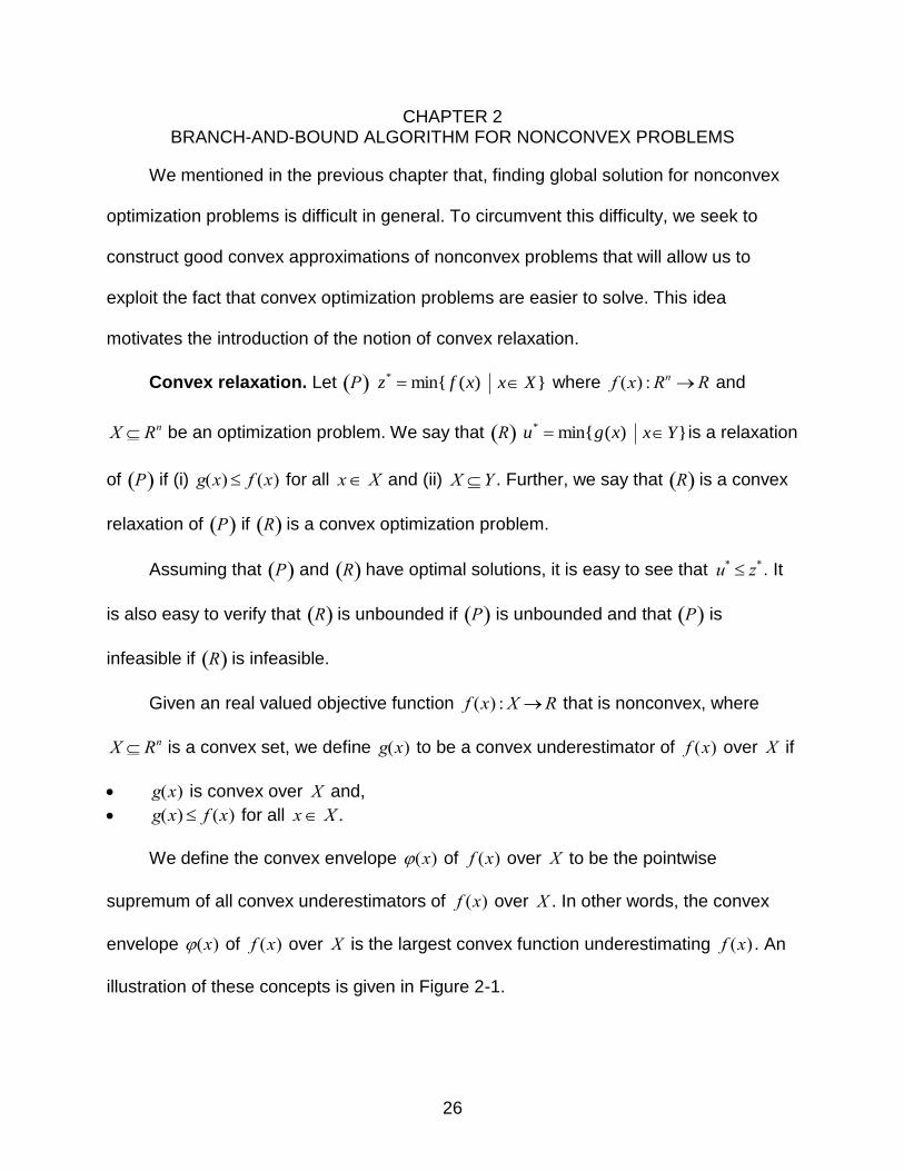
We define the convex envelope

(x) of

f (x) over

X to be the pointwise

supremum of all convex underestimators of

f (x) over

X . In other words, the convex

envelope

(x) of

f (x) over

X is the largest convex function underestimating

f (x) . An

illustration of these concepts is given in Figure 2-1.

27

Figure 2-1. Convex underestimator g(x) and convex envelope φ(x) of the function f(x)

It is clear that if

P )(min{* xfz }Xx is an optimization problem where

X is

a convex set and

f (x) is a nonconvex function, then

R )(min{* xu }Xx is a

convex relaxation of

P where

(x) is the convex envelope of

f (x) over

X .

Given a set

X Rn, we define the convex hull of

X to be the smallest convex set

containing

X . An illustration of this concept is given in Figure 2-2.

A B

Figure 2-2. A) Set X B) Convex hull of X

g(x) )(x

)(xf

28

It is clear that if

P )(min{* xfz }Xx is an optimization problem where

X is a

nonconvex set and

f (x) is a convex function, then

R )(min{* xfu )}(Xconvx is a


P .

In general, given a feasible set S defined by constraints 0)( xgi for ki ,,1 , it is

difficult to find )(Sconv . However it is easily established that xS { },,1,0)( kixi

is a convex relaxation of S where )(xi is the envelope of )(xgi over )(Sconv .

Convex relaxations play an important role in solving many nonconvex optimization

problems. In the next section, we describe how convex relaxations can be combined

with divide-and-conquer principles to give rise to branch-and-bound algorithms for the

global solution of nonconvex problems.

2.1 Branch-and-Bound

Branch-and-bound (BB) is one of the most widely used methods to solve

nonconvex optimization problem to globally optimality. In this method, the initial problem

is relaxed into a convex problem that is solved. If the optimal solution of the relaxation is

also optimal for the initial problem, the process is stopped. Otherwise the problem is

divided into parts (branching) so that stronger relaxations can be built over the pieces

that hopefully have better bounds (bounding).

To illustrate the approach, we consider the following problem:

z* min 22 )10()10(),( yxyxf (2-1)

s.t. 10x

20y

0,0 yx .

29

Because this problem has a concave objective function and a polyhedral feasible

region, it is clear that an optimal solution can be found at an extreme point of the

feasible region of (2-1). It follows then by inspection that

(0,0) is an optimal solution to

the problem. However, we will ignore this to illustrate how the branch-and-bound

algorithm would solve this problem. A possible implementation of the branch-and-bound

algorithm would work as follows.

Step 0. First, the feasible region is relaxed to 0M , which is chosen to be the

convex hull of

{(0,0),(30,0),(0,30)}. This set is a simplex that contains the feasible region

D . For more information about simplices, we refer to [6].

Since the objective function of (2-1) is concave, the affine function coinciding with

),( yxf at the vertices of

M0 is the convex envelope of

f (x,y) over

M0 ; see definition of

concave function in the previous chapter. In particular, the parameters of

(x,y) ax by c can be obtained by solving the system

(0,0) 200,

(30,0) 400,

(0,30) 400 which equates the values of

(x,y) and

f (x,y) at the vertices of

M0 . We

obtain:

200c

10a

10b

and so we conclude that 2001010),( yxyx is a convex underestimator of

22 )10()10(),( yxyxf , i.e., ),(),( yxfyx 0),( Myx . Now, a lower bound to

(2-1) can be found by solving the following linear program

min 2001010),( yxyx (2-2)

s.t. DMyx 0),( .

30

The optimal value of (2-2) is 800 and is achieved at )20,10( . It follows that

z* 800 . Now, observe that the two points )0,0( and )20,10( belong to the feasible

region. Since the feasible region is convex, the segment between them, call it 0MS also

belongs to

M0 . Optimizing

f (x,y) over

S yield ),(min{0 yxf 200}),(0

MSyx ,

which is achieved at the point

x0 (0,0). Since

(0,0) is feasible with value

200, we

conclude that

z* 200 . Combining these observations, we can say that

800 z* 200. Because the gap between upper and lower bound is large, we will

subdivide the problem into smaller pieces.

Step 1. In this step, we partition

M0 into two other simplices

M1,1 conv{(0,0),(10,20),(0,30)} and

M1,2 conv{(0,0),(10,20),(30,0)}. After partitioning

M0 , we check that each one of these intersects the feasible region, i.e., DM 1,1 or

DM 2,1 . If not then it is unnecessary to investigate the corresponding simplex

further since it cannot contain the optimal solution (as it does not even contain a

feasible solution). In classical branch-and-bound terminology, we prune the

corresponding branch because we know that a solution to the actual problem cannot lie

in that branch.

In our example, both

M1,1 and

M1,2 intersect

D and so, they both must be

considered. We then must construct a convex relaxation of (2-1) over

M1,1 and

M1,2 .

)}30,0(),20,10(),0,0{(1,1 convM

)}0,30(),20,10(),0,0{(2,1 convM

)}30,0(),0,30(),0,0{(0 convM

31

Proceeding as before, we compute

1,1 ax by c and

1,2 ax by c. We calculate

the coefficients of these envelopes as explained in the previous step to obtain

1,1 30x 10y 200 and 20010102,1 yx . We now can solve convex relaxations of

(2-1) over

M1,1 and

M1,2 respectively by solving linear programs. We obtain the lower

bounds

1,1 400 achieved at

(0,20) and

1,2 300 achieved at

(10,0). Therefore, we

conclude that

z* 1 min(1,1,1,2) 400. Looking for feasible solutions in

M1,1 and

M1,2 ,

we obtain that

1,1 min f (SM1,1) 200 is achieved at )0,0( and )(min

2,12,1 MSf

200 is achieved at )0,0( , where, )}20,10(),20,0(),0,0{(1,1MS and

)}20,10(),0,10(),0,0{(2,1MS . This leads to an overall upper bound of

200),min( 2,11,11 achieved at )0,0(1 x . Because 11 , we will partition the

problem further.

Step 2. In the next iteration, we check first whether any of the previous branches

can be pruned on the basis that 1,1 or 2,1 1 . In fact, in such a situation, the best

possible solution in the branch is inferior to one already discovered in the tree and

therefore cannot be optimal. This step is one of the fundamental features of branch-and-

bound algorithms that allows entire portions of the feasible region to remain unexplored

on the basis that they cannot possibly contain an optimal solution.

In our case, the best solution found so far only has value

200 and therefore no

pruning occur at this stage. We must, therefore partition 1,1M into 1,2M and 2,2M and to

partition 1,1M into 3,2M and 4,2M so as to define

)}20,10(),20,0(),0,0{(1,2 convM ,

32

)}20,10(),20,0(),30,0{(2,2 convM ,

)}20,10(),0,10(),0,0{(3,2 convM ,

)}20,10(),0,10(),0,30{(4,2 convM .

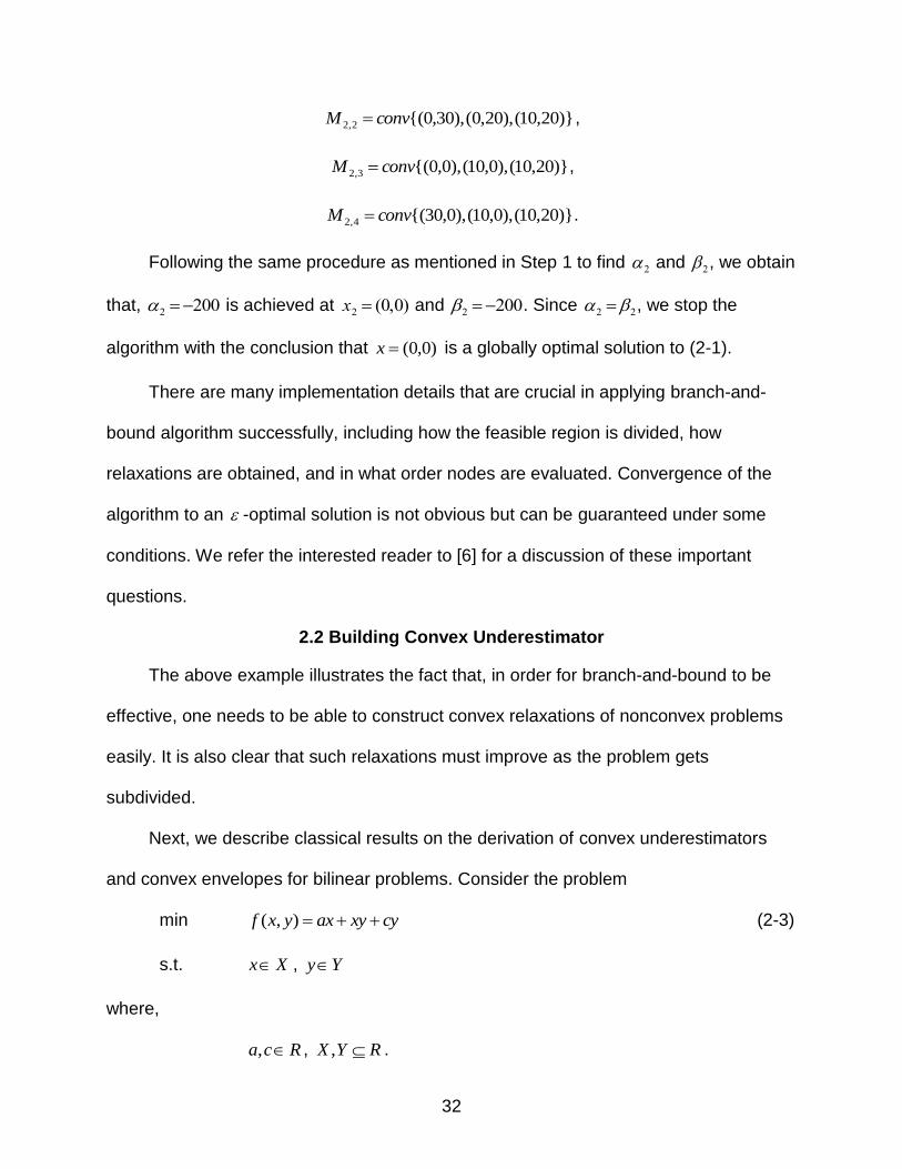
Following the same procedure as mentioned in Step 1 to find

2 and

2, we obtain

that,

2 200 is achieved at

x2 (0,0) and

2 200. Since

2 2, we stop the

algorithm with the conclusion that )0,0(x is a globally optimal solution to (2-1).

There are many implementation details that are crucial in applying branch-and-

bound algorithm successfully, including how the feasible region is divided, how

relaxations are obtained, and in what order nodes are evaluated. Convergence of the

algorithm to an -optimal solution is not obvious but can be guaranteed under some

conditions. We refer the interested reader to [6] for a discussion of these important

questions.

2.2 Building Convex Underestimator

The above example illustrates the fact that, in order for branch-and-bound to be

effective, one needs to be able to construct convex relaxations of nonconvex problems

easily. It is also clear that such relaxations must improve as the problem gets

subdivided.

Next, we describe classical results on the derivation of convex underestimators

and convex envelopes for bilinear problems. Consider the problem

min cyxyaxyxf ),( (2-3)

s.t. Xx , Yy

where,

Rca , , RYX , .

33

Let ),( yxK underestimate the function

f (x,y) over K where K is any convex set

in domain of the function. Then it can be argued that

cyyxaxyx KK ),(),( (2-4)

where ),( yxK denotes the convex underestimator of xy over K . Now, it requires

designing a procedure to build ),( yxK .

Let },:),{( yxyxp , be a hyper-rectangle that contains the feasible

region, and let

pi {(xi,yi) :i xi i,i yi i} be such that

nn pppppp 1321 . This type of partitioning is used in the branch-and-bound

algorithm for BP developed by Al-Khayyal and Falk [1]. We seek to develop relaxations

of the terms

xi,yi over

pi .

We can safely say that:

xi i 0 (2-5)

and

yi i 0 . (2-6)

Multiplying (2-5) and (2-6) gives,

xiyi ixi iyi ii . In other words,

f1(xi,yi) ixi iyi ii underestimates

xiyi over

pi .

Similarly,

0 ii x (2-7)

and

0 ii x . (2-8)

Multiplying (2-7) and (2-8) gives iiiiiiii yxyx . In other words,

iiiiiiii yxyxf ),(2 also underestimates

xiyi over

pi .

34

Since the pointwise supremum of convex underestimators of a function also

underestimates the function, we conclude that

)},(),,(max{),( 21 iiiiip yxfyxfyx (2-9)

is a convex underestimator of

xiyi over

pi .

It can be shown that (2-9) forms the convex envelope of

xiyi over

pi . We refer to

Al-Khayyal and Falk [1] for a proof.

2.3 Factorable Relaxations

For more general functions, finding convex envelopes is typically a difficult

problem. However, several techniques have been proposed to derive convex

underestimators. We describe one such technique next that was initially proposed by G.

P. McCormick [9].

This technique applies to factorable functions that can be obtained recursively,

using sums and products of a family of univariate base functions whose convex

envelopes are known. The family of base functions can contain polynomial, exponential

or trigonometric functions. The technique proceeds by breaking down the initial function

into its constituent terms and then approximating these terms individually. The

technique can be used to obtain convex underestimators of objective functions but also

can be used to construct convex relaxations of nonconvex constraints as

˜ f (x) r is a


f (x) r whenever

˜ f (x) is a convex underestimator of

f (x) . To

illustrate the ideas behind the factorable relaxation technique, we consider the following

constraint:

f (x,y,z) (x y)2 z 3xy 2 4 (2-10)

35

where, it is known otherwise that variables belong to the unit hypercube, i.e., 10 x ,

10 y , and 10 z .

Our goal is to find a good convex underestimator

(x,y,z) of

f (x,y,z) over 3]1,0[ as

(x,y,z) 4 will provide a convex relaxation to

f (x,y,z) 4 . At first glance, it may

appear difficult to devise such a convex underestimator. For this reason, we will start

breaking down the function into components until we obtain terms that are sufficiently

simple to approximate.

To break down

f (x,y,z), we introduce two new variables

u1 and

u2 as

u1 (x y)2z (2-11)

u2 xy 2. (2-12)

Still, it is difficult to relax these terms and hence we will break them down further

by introducing new variables

u3 and

u4 as

u3 x y,

u4 u3

2,

u1 u4z. Each of these

terms is then relaxed as summarized in Table 2-1.

Table 2-1. Sub-problems obtained after breaking down

u1 (x y)2z

Sub-problem Convex relaxation

u3 x y This constraint is convex and

1 u3 1.

u4 u3

2 As shown in the Figure 2-3, the feasible region defined by this constraint is not

convex over 11 3 u . It can be

observed from the figure that

u3

2 u4 1

provides a convex relaxation of the feasible set defined by this constraint.

u1 u4z As discussed earlier in this chapter, we can use standard techniques to find a convex relaxation to this expression; see convex envelope for bilinear problems, which yields

u1 u4 ,

u1 z ,

u1 u4 z1

and

u1 0.

36

Figure 2-3. Convex relaxation of the sub-problem

u4 u3

2

A convex relaxation for the set if feasible solutions to equation

u1 (x y)2z for

3]1,0[),,( zyx can therefore be written as:

u3 x y (2-13)

u4 u3

2 (2-14)

u4 1 (2-15)

u1 u4 (2-16)

u1 z (2-17)

u1 u4 z1 (2-18)

u1 0 . (2-19)

For

u2, we proceed similarly and introduce new variable

u5 as

u5 y2,

u2 u5x .

Each of these terms is then relaxed as summarized in Table 2-2.

(u3)2

u3

37

Table 2-2. Sub-problems obtained after breaking down

u2 xy 2

Sub-problem Convex relaxation

u5 y2 As shown in Figure 2-4, the feasible region defined by this constraint is not convex over 10 y . It can be observed

from the figure that

y2 u5 y provides a

convex relaxation of the feasible set defined by this constraint.

u2 u5x Similarly to the previous case, a convex relaxation is given by

u2 u5,

u2 x ,

u2 u5 x 1 and

u2 0.

Figure 2-4. Convex relaxation of the sub-problem

u5 y2

A convex relaxation for the set of feasible solution to equation

u2 xy 2 for

2]1,0[),( yx can therefore be written as:

u5 y2 (2-20)

u5 y (2-21)

u2 u5 (2-22)

u2 x (2-23)

u2 u5 x 1 (2-24)

y2

1

y

38

u2 0, (2-25)

together with

10 x , 10 y , 10 z . (2-26)

Combining (2-13) – (2-19) and (2-20) – (2-26) with

f (x,y,z) u1 3u2 4 (2-27)

provides a convex relaxation for the set of feasible solution to constraint (2-10).

The ideas presented here can be applied general factorable functions. We refer to

Tawarmalani and Sahinidis [11] for a more detailed description. Factorable relaxations

are used in commercial global optimization software such as Baron and Lindoglobal.

39

CHAPTER 3 CONVEX RELAXATIONS FOR BILINEAR COVERING SETS

3.1 Motivation

As discussed in the previous chapters, building strong convex relaxations is key in

solving many complex nonconvex problems to global optimality. We next demonstrate

through two examples that multilinear covering constraints of the form

x i, j

j1

m

d

i1

n

(3-1)

occur in practical problems. This will be the primary motivation for our later polyhedral

studies.

3.1.1 Strassen’s Algorithm

The problem of multiplying two matrices of dimension nn is a fundamental

problem in linear algebra. When multiplying matrix

nj

niijaA

,,1

,,1

with

nj

niijbB

,,1

,,1

,

we create a new matrix

nj

niijcC

,,1

,,1

whose components ijc are obtained through the formula kj

n

k

ikij bac

1

for ni ,,1 and

nj ,,1 .

A straightforward application of the formula shows that it is possible to compute

the product of two nn matrices using 3n multiplications and )1(2 nn additions,

40

resulting in a )( 3nO algorithm. There are, however, algorithms for matrix multiplication

with running time of )( rnO where 3r . Strassen’s algorithm [10] is one such algorithm.

The fundamental idea in Strassen’s algorithm is that, when considering matrices

2221

1211

aa

aa

and

2221

1211

bb

bb,

it is possible to compute their product

2222122121221121

2212121121121111

2221

1211

babababa

babababa

cc

cc

using only 7 multiplications and 18 additions/subtractions. This can be done as follows.

First, we compute:

1T = 2211 aa 2211 bb

2T = 2221 aa 11b

3T = 11a 2212 bb

4T = 22a 1121 bb

` 5T = 1211 aa 22b

6T = 1121 aa 1211 bb

7T = 2212 aa 2221 bb .

Then, we combine these terms as follows:

11c = 7541 TTTT

41

12c = 53 TT

21c = 42 TT

22c = 6321 TTTT .

Because matrices can be block multiplied, a recursive application of the above

equations yields a )(72log

nO algorithm for matrix multiplication.

An important question is that of determining whether such rule can be obtained

systematically. This question can be answered positively as schemes to multiply two

22 matrices using only 7 multiplications corresponds to feasible solutions to a mixed

integer nonlinear problem with constraints:

7

1

0t

skhrigrstghtikt yxz 2,1,,,,, srhgki (3-2)

where,

zijt,xijt,yijt {1,0,1} 2,1, ji and 7,,1t .

In the above model, the variable ijtz represents the coefficient of tT in ijc , ijtx

represents the coefficient of ija in tT , ijty represents the coefficient of ijb in tT ,

ij 1

i j and 2,1, ji , and 0ij ji and 2,1, ji . More precisely, a feasible

solution to Problem (3-2) yields a way of computing C with the 7 multiplications as

tT =

}2,1{, ji

ijijtax

}2,1{, ji

ijijtby ,

with the following additions,

ijc =

7

1t

tijtTz .

Similarly, one could determine if there exists a way of multiplying 33 matrices

42

using 23 multiplications by determining if the following system is feasible or not:

zikt xghtyrst ighrsk 0t1

23

3,2,1,,,,, srhgki (3-3)

where,

zijt,xijt,yijt {1,0,1} 3,2,1, ji and 23,,1t .

1ij

i j , 3,2,1, ji and

ij 0

i j , 3,2,1, ji .

A feasible solution to Problem (3-2) would yield an algorithm for multiplying

3 3

matrix with 23 multiplications instead of 27. Such a feasible solution, in turn, would lead

to a )(233log

nO algorithm for matrix multiplication. A feasible solution to Problem (3-3) can

be found in [7].

The constraints of the above models involve multilinear functions. It is simple to

reformulate them using variables rstghtghrst yxu to transform (3-2) and (3-3) into a

problem containing only bilinear constraints, some of which can be relaxed to form (3-1)

3.1.2 Staff Scheduling Problems

Traditional staff scheduling models also can be formulated as bilinear integer

programs if the shifts are part of the decision variables.

To clarify the idea, consider a problem in which a call center has to ensure that at

least d operators are on duty during time slot t . Operators must be assigned to one of

the k shifts (whose characteristics must be decided) in a way that minimizes the

number of operators used. Shifts are characterized only by their start time. We assume

that shifts are required to contain a sequence of r consecutive time slots of work

followed by 1 time slot of rest, followed by r time slots of work.

To model such problem, we introduce variables tkX as

43

1tkX , if time slot t is part of shift k

0tkX , otherwise.

We introduce tkZ as

1tkZ , if shift k starts at time t

0tkZ , otherwise,

and let kY to represent the number of operators assigned to shift k .

The problem can then be formulated as:

min

K

k

kY1

s.t.

(1)

K

k

tktk dYX1

},,1{ Tt

(2)

T

t

tk rX1

2 },,1{ Kk

(3) tkkit ZX )( },,1{ Kk , },,1{ Tt , }2,,1,1,,1{ rrri

(4) tkkrt ZX 1)( },,1{ Kk , },,1{ Tt

(5)

T

t

tkZ1

1 },,1{ Kk .

In the above model, constraint (1) requires that sufficiently many operators are

present during each time period, constraint (2) imposes that operators work for r2 time

periods, constraints (3) and (4) state that the shift requires work in the period 1,,1 r

and rr 2,,1 , and rest in period r after the beginning of the shift while constraint (5)

requires that the shift has a single starting period. In model (1) - (5), we replace rt

with Trt whenever Trt .

44

In the above model, we see that the constraints that require that sufficiently many

operators are available at any point in time are bilinear and are of the form (3-1). We

also observe that they contain only integer variables.

3.2 Problem Description

As illustrated before in this chapter, constraints of the form:

n

i

ii dyx1

(3-4)

where,

xi {0,1} Ni ,

},,0{ ii uy Ni ,

ui Z Ni ,

nuuuu 321 ,

Zd ,

},,1{ nN

appear in the formulation of several practical problems. It would therefore be useful to

derive convexification procedures for them. Current convexification procedures applied

to this problem would (i) relax integrality and (ii) build convex relaxations by finding

concave overestimators of the product ii yx . This results in a double source of weakness

as (i) it can be seen that integrality makes the convex hull of feasible solutions to (3-4)

polyhedral while the convex hull of the continuous relaxation is not and (ii) the relaxation

dxg )( where g is a concave overestimator of ii yx does not yield the convex hull of

feasible solutions to (3-4). Therefore, we wish to derive expressions for the convex hull

of sets defined by (3-4).

45

We define a polyhedron as the set of feasible solutions to a finite number of

inequalities and equalities:

nRxP { }, dCxbAx (3-5)

where nmRA , mRb , npRC , and pRd . We say that P is bounded if P is

contained in a ball of finite radius. A bounded polyhedron is said to be polytope.

Because the feasible sets of integer bilinear sets are composed of a finite number of

points, the following result can be easily established using Minkowski-Weyl’s Theorem

[13].

We denote the feasible region of Problem (3-4) by B and the convex hull of B by

)(Bconv .

Proposition 3.2.1: The convex hull of the feasible solutions to Problem (3-4) is a

polytope, i.e., )(Bconv is a polytope.

As a first step in the derivation of such convex hulls, we use MATLAB to generate

the convex hulls of sample problems where the values of d and iu are fixed. To this

end, we use the MATLAB function K = convhulln(X) where },,1{ miixX

, and ix s are

the feasible solutions (vectors in n2 dimensions) of Problem (3-4). We restricted

ourselves to small values of n , d , and iu s so that the function K = convhulln(X) works

relatively fast.

During the study of the results produced by MATLAB, we found that the structure

of the convex hull is strongly influenced by the position of d in the sequence

nuuu 21 . Therefore we divide the study of the problem into different cases

depending upon position of d in the sequence. In particular, we define case k to be the

46

case where

uk1 d and

uk d .

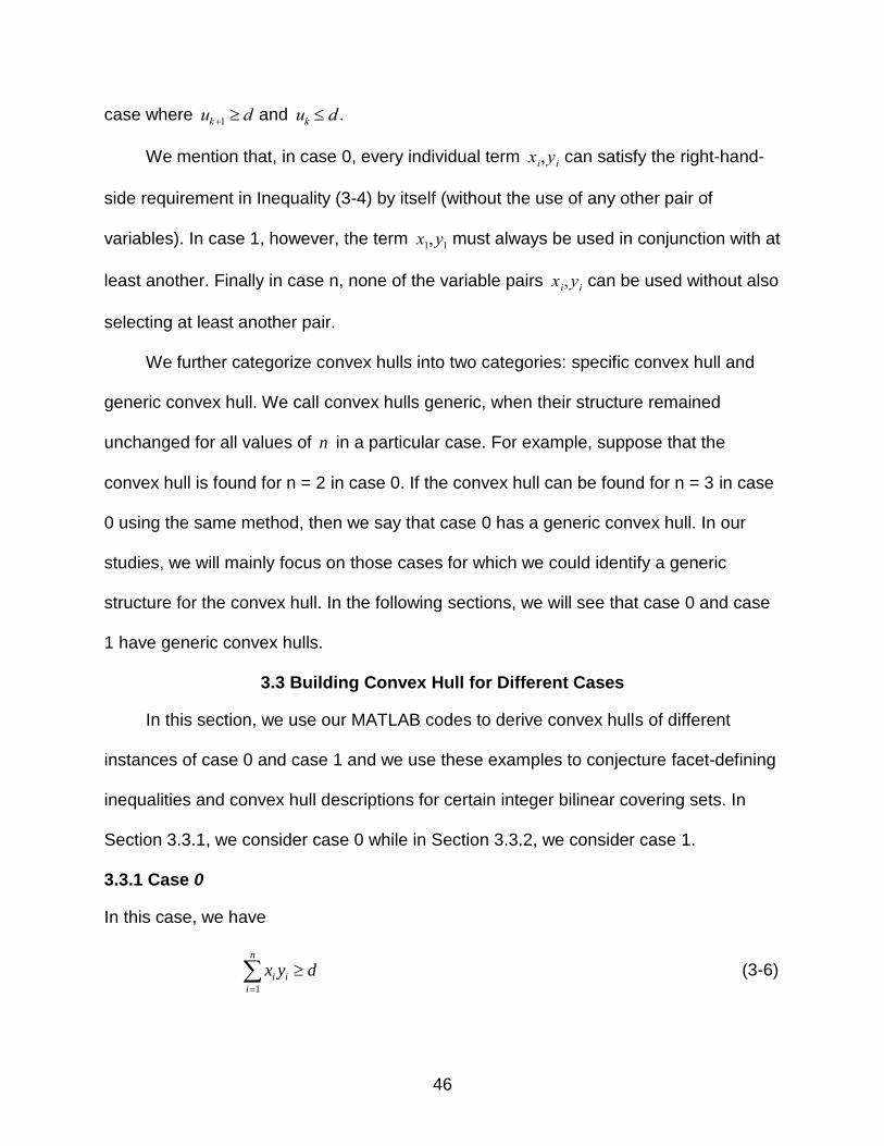
We mention that, in case 0, every individual term

xi,yi can satisfy the right-hand-

side requirement in Inequality (3-4) by itself (without the use of any other pair of

variables). In case 1, however, the term

x1,y1 must always be used in conjunction with at

least another. Finally in case n, none of the variable pairs

xi,yi can be used without also

selecting at least another pair.

We further categorize convex hulls into two categories: specific convex hull and

generic convex hull. We call convex hulls generic, when their structure remained

unchanged for all values of n in a particular case. For example, suppose that the

convex hull is found for n = 2 in case 0. If the convex hull can be found for n = 3 in case

0 using the same method, then we say that case 0 has a generic convex hull. In our

studies, we will mainly focus on those cases for which we could identify a generic

structure for the convex hull. In the following sections, we will see that case 0 and case

1 have generic convex hulls.

3.3 Building Convex Hull for Different Cases

In this section, we use our MATLAB codes to derive convex hulls of different

instances of case 0 and case 1 and we use these examples to conjecture facet-defining

inequalities and convex hull descriptions for certain integer bilinear covering sets. In

Section 3.3.1, we consider case 0 while in Section 3.3.2, we consider case 1.

3.3.1 Case 0

In this case, we have

n

i

ii dyx1

(3-6)

47

where }1,0{ix , },,0{ ii uy , Zui , and Zd with nuuu 21 , du 1 .

3.3.1.1 Problem 1

In Problem (3-6), we set 3d and 2n to obtain:

32211 yxyx (3-7)

where

xi {0,1}, },,0{ ii uy , Zui , 3, 21 uu , and 21 uu .

To use MATLAB, we also need to choose values for 1u and 2u . For 321 uu , we

list all feasible solutions to the problem and find the convex hull using MATLAB function

K = convhulln(x). For this instance, we present all feasible solutions in Table 3-1. These

points were obtained using a code we wrote MATLAB. The code is presented in

Appendix.

Table 3-1. Feasible points for 32211 yxyx and 321 uu

1x 1y 2x 2y

1 3 0 0 1 3 1 0 1 3 0 1 1 2 1 1 1 3 1 1 1 3 0 2 1 1 1 2 1 2 1 2 1 3 1 2 1 3 0 3 0 0 1 3 1 0 1 3 0 1 1 3 1 1 1 3 0 2 1 3 1 2 1 3 0 3 1 3 1 3 1 3

Observe that, in Table 3-1, not all points are necessary to build the convex hull as

some of the points are convex combination of other points. In particular, (1,3,0,1) is a

48

convex combination of (1,3,0,0) and (1,3,0,2) and therefore could be omitted from the

list without altering the convex hull. However, computing convex hulls with these

unnecessary points does not compromise the validity of our approach.

The convex hull of feasible points of Table 3-1 generated using MATLAB, is presented

in Table 3-2.

Table 3-2. Convex Hull for 32211 yxyx

Convex hull (for restricted problem) Convex hull (for original problem)

333 21 xx 333 21 xx

33 21 xy 33 21 xy

33 21 yx 33 21 yx

321 yy 321 yy

1, 21 xx 1, 21 xx

3, 21 yy 11 uy , 22 uy

Repeating the computation for various values of 1u and 2u we conjecture the

convex hull for the original problem (3-7), presented in the right side of Table 3-2.

Intuitively, this works because the convex hull of Problem (3-4) has two kinds of

inequalities: lower bounding and upper bounding. Lower bounding inequalities do not

change as long as upper bounding inequalities do not interact with them. Limit cases

are encountered when an upper bounding inequality and a lower bounding inequality of

the convex hull meet at a vertex.

3.3.1.2 Problem 2

We consider now a case larger right-hand-side value. In particular, we set 4d

and 2n in Problem (3-6) to obtain:

42211 yxyx (3-8)

where

xi {0,1}, },,0{ ii uy , Zui , 4, 21 uu , and 21 uu .

49

To conjecture the convex hull of this problem, we apply the same procedure as

before. We first restrict 421 uu so that we can find the convex hull of the restricted

problem easily. After finding it, we replace the upper bounds on 1y and 2y with 1u and

2u respectively.

The convex hull of feasible points generated using MATLAB, is presented in Table 3-3.

Table 3-3. Convex Hull for 42211 yxyx


444 21 xx 444 21 xx

44 21 xy 44 21 xy

44 21 yx 44 21 yx

421 yy 421 yy

1, 21 xx 1, 21 xx

4, 21 yy 11 uy , 22 uy

In the right side of the table, we present our conjecture for the convex hull when 1u

and 2u are general. From the results of Table 3-2 and Table 3-3, we next infer the

general form for the convex hull of case 0 when 2n .

3.3.1.3 Convex hull for n=2

We compare the inequalities obtained in Problem 1 and 2. Inequalities 333 21 xx

and 444 21 xx are similar, and the difference can be easily attributed to d . We

therefore infer that, ddxdx 21 is a required inequality for any value of d . We will

verify this claim later in this chapter. Second we observe that inequalities 33 21 xy

and 44 21 xy are similar and have an obvious dependence on d that can be

generalized to ddxy 21 . Similarly, inequalities 33 21 yx and 44 21 yx can be

generalized to dydx 21 . Regarding this second and third inequalities, it can be

50

argued that if anyone of them is a valid inequality then the other one is also valid,

because of symmetry. Fourth similar inequalities are 321 yy and 421 yy which

can be extended in terms of d to dyy 21 .

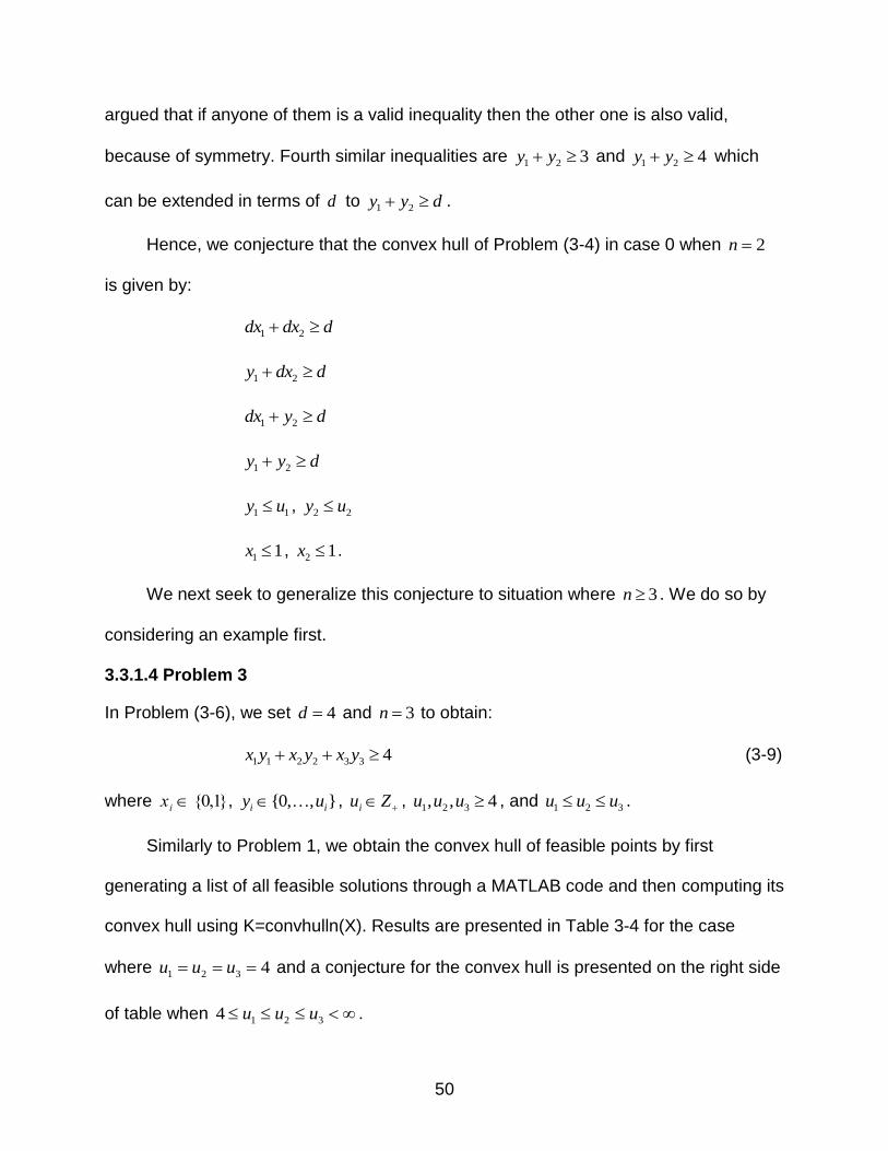
Hence, we conjecture that the convex hull of Problem (3-4) in case 0 when 2n

is given by:

ddxdx 21

ddxy 21

dydx 21

dyy 21

11 uy , 22 uy

11 x , 12 x .

We next seek to generalize this conjecture to situation where 3n . We do so by

considering an example first.

3.3.1.4 Problem 3


4332211 yxyxyx (3-9)

where

xi {0,1}, },,0{ ii uy , Zui , 4,, 321 uuu , and 321 uuu .

Similarly to Problem 1, we obtain the convex hull of feasible points by first

generating a list of all feasible solutions through a MATLAB code and then computing its

convex hull using K=convhulln(X). Results are presented in Table 3-4 for the case

where 4321 uuu and a conjecture for the convex hull is presented on the right side

of table when 3214 uuu .

51

Table 3-4. Convex Hull for 4332211 yxyxyx


4444 321 xxx 4444 321 xxx

444 321 yxx 444 321 yxx

444 321 xyx 444 321 xyx

444 321 xxy 444 321 xxy

44 321 yyx 44 321 yyx

44 321 yxy 44 321 yxy

44 321 xyy 44 321 xyy

4321 yyy 4321 yyy

1,,0 321 xxx 1,,0 321 xxx

4,,0 321 yyy 110 uy , 220 uy , 330 uy

3.3.1.5 Convex hull for case 0

The results of Table 3-4 combined with those of Table 3-2 and Table 3-3, suggest

the following form for )(Bconv :

dyxdSNj

ji

Si

\

NS where },,1{ nN (3-10)

1ix Ni (3-11)

ii uy Ni (3-12)

0ix Ni for 3n (3-13)

0iy Ni for 3n (3-14)

3.3.2 Case 1

We now focus on developing a conjecture for the convex hull of integer bilinear

covering set in case 1. In this case, we consider the set of feasible solutions to

n

i

ii dyx1

(3-15)

where

xi {0,1}, },,0{ ii uy , Zui , and Zd when nuuu 21 , we assume

52

here that du 1 , du 2 .

3.3.2.1 Problem 4


4332211 yxyxyx (3-16)

where

xi {0,1}, },,0{ ii uy , Zui , 41 u , 4, 32 uu , and 321 uuu .

Similarly to Section 3.3.1.1, we will build the convex hull for Problem (3-16). We

consider two cases. First, we set 31 u and 4, 32 uu . Second, we set

u1 2 and

4, 32 uu . After building the convex hulls of these two instances, we will conjecture a

convex hull description for the general problem. Results are presented in Table 3-5.

Table 3-5. Convex Hull for 4332211 yxyxyx in case 1

Convex hull ( 31 u

and 4, 32 uu )

Convex hull (

u1 2 and

4, 32 uu )

Convex hull (for original problem)

443 321 yxx

2x1 4x2 y3 4 44 3211 yxxu

443 321 xyx

2x1 y2 4x3 4 44 3211 xyxu

43 321 yyx

2x1 y2 y3 4 43211 yyxu

44 321 yxy 44 321 yxy 44 321 yxy

44 321 xyy 44 321 xyy 44 321 xyy

4321 yyy 4321 yyy 4321 yyy

132 xx

x2 x3 1

x2 x3 1

132 yx

2x2 y3 2 )4()4( 1321 uyxu

132 xy

y2 2x3 2 )4()4( 1312 uxuy

1,,0 321 xxx 1,,0 321 xxx 1,,0 321 xxx

30 1 y 4,0 32 yy 20 1 y 4,0 32 yy 110 uy , 220 uy ,

330 uy

Comparing the inequalities, we present, in the right column a conjecture for the

convex hull description of feasible solutions to Problem (3-16).

We now examine the dependence of this convex hull on the right-hand-side value d .

53

3.3.2.2 Problem 5

In Problem (3-6), we now set

d 5 and 3n to obtain

x1y1 x2y2 x3y3 5 (3-17)

where

xi {0,1}, },,0{ ii uy , Zui ,

u1 5,

u2,u3 5, and 321 uuu .

Similarly to Section 3.3.2.1, we consider two sets of values for the bounds

321 ,, uuu . The first choice is obtained by setting

u1 4 and

u2,u3 5. The second is

obtained by setting

u1 3 and

u2,u3 5. Results are presented in Table 3-6.

Table 3-6. Convex Hull for

x1y1 x2y2 x3y3 5

Convex hull (

u1 4 and

u2,u3 5)

Convex hull (

u1 3 and

u2,u3 5)

Convex hull (for original problem)

554 321 yxx 553 321 yxx 55 3211 yxxu

554 321 xyx 553 321 xyx 55 3211 xyxu

54 321 yyx

3x1 y2 y3 5

u1x1 y2 y3 5

55 321 yxy

y1 5x2 y3 5

y1 5x2 y3 5

55 321 xyy

y1 y2 5x3 5

y1 y2 5x3 5

5321 yyy

y1 y2 y3 5

y1 y2 y3 5

132 xx 132 xx

x2 x3 1

132 yx 22 32 yx

(5 u1)x2 y3 (5 u1)

132 xy 22 32 xy

y2 (5 u1)x3 (5 u1)

1,,0 321 xxx 1,,0 321 xxx 1,,0 321 xxx

40 1 y 5,0 32 yy 30 1 y 5,0 32 yy 110 uy , 220 uy ,

330 uy

Comparing the inequalities, we present, in the right column a conjecture for the

convex hull description of feasible solutions to Problem (3-17).

3.3.2.3 Convex hull for n = 3

We are now ready to conjecture a polyhedral description of the convex hull of

integer bilinear covering sets in case 1. Comparing inequalities with similar structure for

Problems 4 and 5, we conjecture the following description of the convex hull of case 1

54

for n = 3.

Table 3-7. Convex Hull for

x1y1 x2y2 x3y3 d

Convex hull ( 4d ) Convex hull (

d 5) Convex hull (

d)

44 3211 yxxu

u1x1 5x2 y3 5

u1x1 dx2 y3 d (1)

44 3211 xyxu

u1x1 y2 5x3 5

u1x1 y2 dx3 d (2)

43211 yyxu

u1x1 y2 y3 5

u1x1 y2 y3 d (3)

44 321 yxy

y1 5x2 y3 5

y1 dx2 y3 d (4)

44 321 xyy

y1 y2 5x3 5

y1 y2 dx3 d (5)

4321 yyy

y1 y2 y3 5

y1 y2 y3 d (6)

x2 x3 1

x2 x3 1

x2 x3 1 (7)

)4()4( 1321 uyxu

(5 u1)x2 y3 (5 u1)

(d u1)x2 y3 (d u1)(8)

)4()4( 1312 uxuy

y2 (5 u1)x3 (5 u1)

y2 (d u1)x3 (d u1)(9)

1,,0 321 xxx 1,,0 321 xxx 1,,0 321 xxx (10)

110 uy ,

220 uy , 330 uy 110 uy ,

220 uy , 330 uy 110 uy , 220 uy ,

330 uy (11)

3.3.2.4 Convex hull for case 1

We next discuss each of the inequalities in Table 3-7 so as to see how they can be

generalized to problems with

n pairs of variables.

First, we observe the inequality

x i 1i 2

n

(3-18)

is always part of the description; see (7). As we discussed before,

x1y1 alone cannot

meet the right-hand-side of Problem (3-15): one of the other

xiyi has to be active. This

argument holds for any value of

n. Hence, we conjecture that the inequality (3-18) is

part of the convex hull description for any value of

n in case 1.

Second, inequalities (1), (2), (3), (4), (5), and (6) suggest that

dyxaSNj

ji

Si

i \

(3-19)

55

where, },,1{ nN , NS , },,2{ nS , and where },min{ dua ii are part of the

convex hull description. Hence, we conjecture that the family of inequalities (3-19) is

part of the description of )(Bconv for any value of

n in case 1.

To generalize (8) and (9), we write

1

\

1)( udyxudRNj

ji

Ri

(3-20)

where, },,2{ nN , NRNR \, .

Inequality (3-20) can be interpreted in light of Problem (3-6) as an application of

case 0 over variables )()( 22 nn yxyx when

x1y1 are set to their maximum values, with

the exception of inequalities based on ØR and Ø\ RN , since the cases ØR and

Ø\ RN are already handled in (3-18) and (3-19). This argument also holds true for

any value of

n in case 1.

As a result of the above discussion, we conjecture that case 1 has a generic

convex hull of the form:

x i 1i 2

n

(3-21)

dyxaSNj

ji

Si

i \

(3-22)

1

\

1)( udyxudRNj

ji

Ri

(3-23)

1ix Ni (3-24)

ii uy Ni (3-25)

0ix Ni (3-26)

0iy Ni (3-27)

56

where, },,1{ nN , },,2{ nN , NS , NS , NRNR \, , and where

},min{ dua ii .

3.4 Facet-Defining Inequalities and Convex Hulls

As described in Section 3.2, the convex hull of integer bilinear covering sets is

polyhedral. To study further the polyhedral structure of these sets, we next describe

some basic notions about polyhedra and polytopes that we will use in the remainder of

this thesis. We focus on polyhedra of the form:

nRxP { }bAx . (3-28)

Not all inequalities in the definition of a polyhedron P are necessary in describing

P . In order to differentiate the inequalities that are necessary from those that are not,

we introduce a few definitions; we refer to [3] for more details.

Affine independence. Points kxxx ,,, 21 in nR are affinely independent if the

system

01

i

k

i

ix ,

and

01

k

i

i

has 021 k as unique solution.

Next we introduce the concept of dimension of a polyhedron P . The dimension of

P ( Pdim ) is one less than the maximum number of affinely independent points in P . A

polyhedron nRP is said to be full-dimensional if nP dim . An inequality kk bxA is

said to valid for P if

57

kk bxA Px

or equivalently if

xAkmax{ kbPx } .

Given a valid inequality kk bxA for a polyhedron P , we define the face of P

induced by kk bxA to be PxFKK bA {),( }kk bxA . A valid inequality kk bxA for P is

said to be facet-defining for P if 1dimdim ),( PFKK bA . In other words, kk bxA is a

facet-defining inequality for P if there exists Pdim affinely independent points in

),( KK bAF .

Given a full-dimensional polyhedron nRP and a valid inequality kk bxA , proving

that kk bxA is a facet-defining inequality simply requires displaying n affinely

independent points in ),( KK bAF . Several variants of the idea have been proposed that are

sometimes easier to use in practice. We refer the interested reader to [2] for a

description.

3.4.1 Facet-Defining Inequality for Case 0

In our previous section, we conjectured that )(Bconv in case 0 is given by:

dyxdSNj

ji

Si

\

NS (3-29)

1ix Ni (3-30)

ii uy Ni (3-31)

0ix Ni for 3n (3-32)

0iy Ni for 3n (3-33)

where, },,1{ nN .

58

We will show next that these inequalities are facet-defining for )(Bconv . To this

end, we first show that inequalities (3-29), (3-30), (3-31), (3-32), and (3-33) are valid for

B and therefore for )(Bconv . It is easily verified that )(Bconv is full-dimensional when

2n . When 1n , the set B is trivial, i.e., dyx 11 where }1,0{1x , },,0{ 11 uy has a

convex hull that is given by

11 x

and

11 uyd .

This shows that for 1n , )(Bconv is not full-dimensional.

Proposition 3.4.1.1: Inequalities (3-30), (3-31), (3-32), and (3-33) are valid inequalities

for B

Proof: Inequalities (3-30), (3-31), (3-32), and (3-33) are valid for B since they belong to

the initial description of the problem. ■

Proposition 3.4.1.2: Inequality (3-29) is valid for B .

Proof: Consider any feasible solution ),( yx

s.t.

n

i

ii dyx1

(3-34)

where

xi {0,1}, and },,0{ ii uy . Denote },,,{ 21 nxxxx and },,,{ 21 nyyyy .

Case 1: For ØS , Inequality (3-29) reduces to

dyNj

j

.

The inequality is valid for B since

dyxyNj

jj

Nj

j

59

where the first inequality holds since

Nj

jj

Nj

j yxy and the second inequality holds

because of (3-34).

Case 2: For NS , Inequality (3-29) reduces to

ddxNi

i

or equivalently

1Ni

ix .

This inequality is clearly valid for B as, when 0Ni

ix ,

dyxNi

ii

0 .

Case 3: For ØS , Ø\ SN .

We consider two subcases.

Case 3a: Assume that the solution ),( yx of B satisfies

Si

ix 1. Then

dxdyxd i

SiSNj

ji

Si

\

,

showing that ),( yx satisfies (3-29).

Case 3b: Assume that the solution ),( yx of B satisfies

Si

ix 0 . It follows from

(3-34) that if

Si

ix 0 then

SNj

j dy\

. Then

dyyxdSNj

j

SNj

ji

Si

\\

,

showing that ),( yx satisfies (3-29). ■

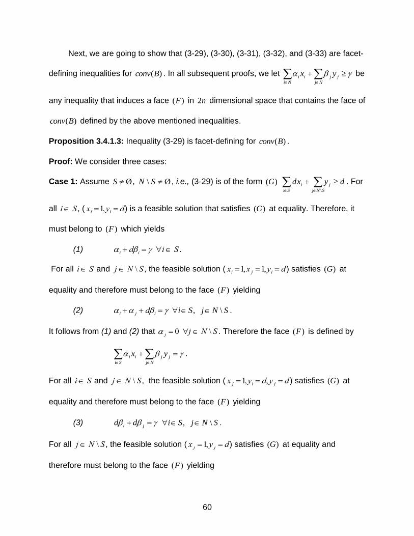
60

Next, we are going to show that (3-29), (3-30), (3-31), (3-32), and (3-33) are facet-

defining inequalities for )(Bconv . In all subsequent proofs, we let Nj

jji

Ni

i yx be

any inequality that induces a face )(F in n2 dimensional space that contains the face of

)(Bconv defined by the above mentioned inequalities.

Proposition 3.4.1.3: Inequality (3-29) is facet-defining for )(Bconv .

Proof: We consider three cases:

Case 1: Assume ØS , Ø\ SN , i.e., (3-29) is of the form )(G dyxdSNj

ji

Si

\

. For

all

i S , (

xi 1,yi d) is a feasible solution that satisfies )(G at equality. Therefore, it

must belong to )(F which yields

(1)

i di

i S .

For all

i S and

j N \ S , the feasible solution (

xi 1,x j 1,yi d ) satisfies )(G at

equality and therefore must belong to the face )(F yielding

(2)

i j di ,Si SNj \ .

It follows from (1) and (2) that

j 0

j N \ S . Therefore the face )(F is defined by

Nj

jji

Si

i yx .

For all

i S and


x j 1,yi d,y j d ) satisfies )(G at


(3) ji dd ,Si SNj \ .

For all


x j 1,y j d) satisfies )(G at equality and

therefore must belong to the face )(F yielding

61

(4)

d j

j N \ S or

j

d.


i 0

i S , and so the face )(F is defined by

SNj

ji

Si

i yd

x\

.

For all

i S , the feasible solution (

xi 1,yi d) satisfies )(G at equality and therefore

must belong to the face )(F yielding

(5)

i

i S

and so the face )(F is defined by

SNj

ji

Si

yd

x\

,

which shows that the inequality defining )(F is a scalar multiple of )(G .

Case 2: Assume ØS , Inequality (3-29) reduces to )(G dyNj

j

. For all

j N ,

(

x j 1,y j d) is a feasible solution that satisfies )(G This yields

(1)

j d j

j N .

For all

i N,

j N , and

i j , the feasible solution (

xi 1,x j 1,y j d ) satisfies )(G at


(2)

i j d j ,Ni jiNj , .


i 0

i N . Therefore face )(F is defined by

Nj

jj y .

For all

j N , the feasible solution (

x j 1,y j d) satisfies )(G at equality and therefore


62

(3)

d j

j N or

j

d


Nj

jyd

,

which shows that the inequality defining )(F is a scalar multiple of )(G .

Therefore dyNj

j

is a facet-defining inequality for )(Bconv .

Case 3: For Ø\ SN , Inequality (3-29) reduces to )(G ddxNi

i

. For all

i N ,

(

xi 1,yi d) is a feasible solution that satisfies )(G at equality and therefore must

belong to the face )(F yielding

(1)

i di

i N .

For all

i N,

j N , and

i j , the feasible solution (

xi 1,yi d,y j d ) satisfies )(G at


(2)

i di d j ,Ni jiNj , .


j 0

j N . Therefore the face )(F is defined by

Ni

ii x .

For all

i N, the feasible solution (



(3)

i

i N

and so the face )(F is defined

Ni

ix ,

63

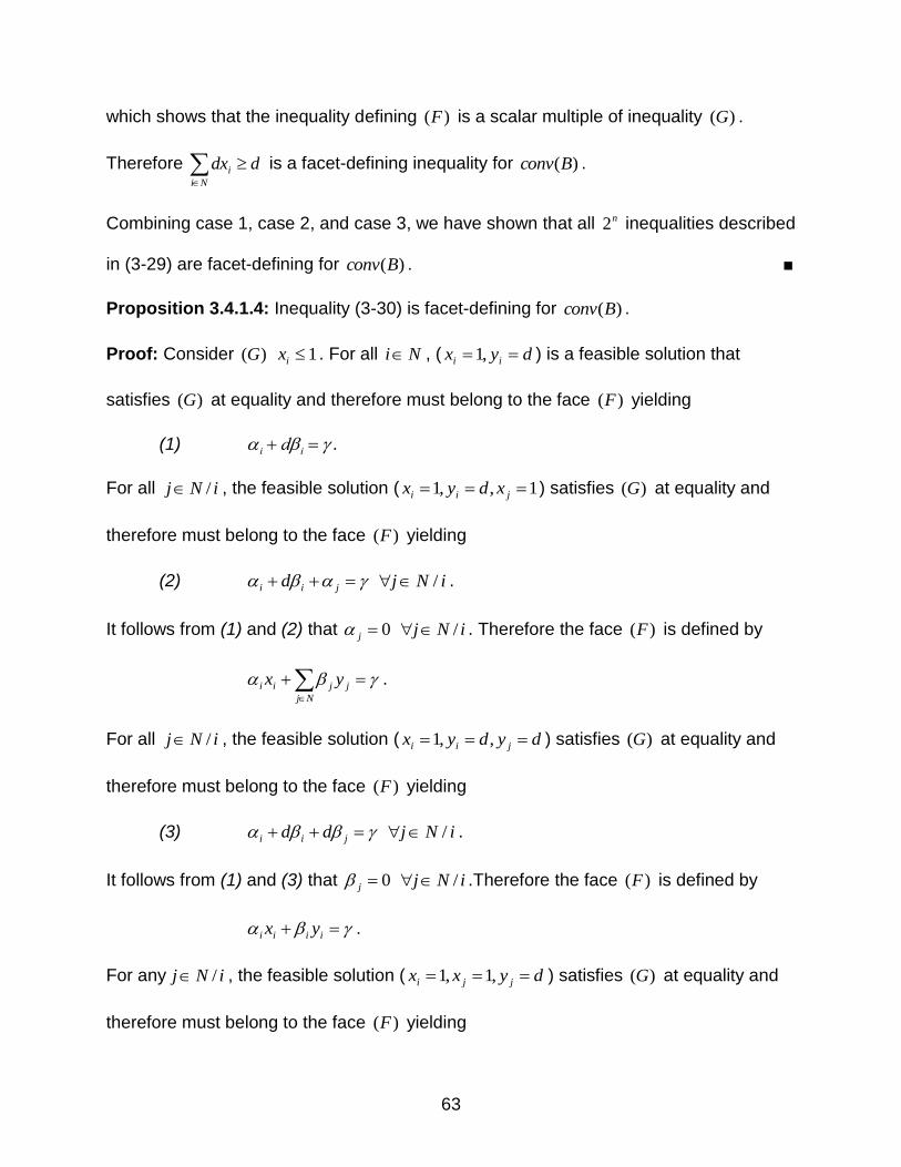
which shows that the inequality defining )(F is a scalar multiple of inequality )(G .

Therefore ddxNi

i

is a facet-defining inequality for )(Bconv .

Combining case 1, case 2, and case 3, we have shown that all n2 inequalities described

in (3-29) are facet-defining for )(Bconv . ■


Proof: Consider )(G 1ix . For all Ni , ( dyx ii ,1 ) is a feasible solution that

satisfies )(G at equality and therefore must belong to the face )(F yielding

(1)

i di .

For all iNj / , the feasible solution ( 1,,1 jii xdyx ) satisfies )(G at equality and


(2) jii d iNj / .

It follows from (1) and (2) that 0j iNj / . Therefore the face )(F is defined by

Nj

jjii yx .

For all iNj / , the feasible solution ( dydyx jii ,,1 ) satisfies )(G at equality and


(3) jii dd iNj / .

It follows from (1) and (3) that 0j iNj / .Therefore the face )(F is defined by

iiii yx .

For any iNj / , the feasible solution ( dyxx jji ,1,1 ) satisfies )(G at equality and


64

(4) i .

It follows from (1) and (4) that 0i , therefore the face )(F is defined by

1ix .

This shows that 1ix is facet-defining for )(Bconv . ■


Proof: Consider )(G ii uy . For Ni , ( iii uyx ,1 ) is a feasible solution that


(1) iii u .

For all iNj / , the feasible solution ( 1,,1 jiii xuyx ) satisfies )(G at equality and


(2) jiii u iNj / .


Nj

jjii yx .

For all iNj / , the feasible solution ( dyuyx jiii ,,1 ) satisfies )(G at equality and


(3) jiii du iNj / .


iiii yx .

For all iNj / , the feasible solution ( dyxuy jjii ,1, ) satisfies )(G at equality and


65

(4) iiu .

It follows from (1) and (4) that 0i , therefore the face )(F is defined by

i

i

yu

or equivalently

ii uy .

This shows that ii uy is facet-defining for )(Bconv . ■

Proposition 3.4.1.6: For 3n , Inequality (3-32) is facet-defining for )(Bconv .

Proof: We use the direct approach of finding n2 affinely independent points in the face

induced by 0ix . We assume without loss of generality that we consider 01 x . The

following n2 points for 3n

),( yx = ),( 22 dee

),( yx = ),( 22 deee i for ni ,,3

),( yx = ),( 22 idedee for ni ,,4,3,1

),( yx = ),( 323 dedee

),( yx = ),( 33 dee

are affinely independent and satisfy 01 x at equality. This shows that 01 x is facet-

defining for )(Bconv . ■

Proposition 3.4.1.7: For 3n , Inequality (3-33) is facet-defining for )(Bconv .

Proof: We use the direct approach of finding n2 affinely independent points in the face

induced by 0iy . We assume without loss of generality that we consider 01 y . The

following n2 points for 3n

66

),( yx = ),( 22 dee

),( yx = ),( 22 deee i for ni ,,4,3,1

),( yx = ),( 22 idedee for ni ,,3

),( yx = ),( 323 dedee

),( yx = ),( 33 dee

are affinely independent and satisfy 01 y at equality. This shows that 01 y is facet-

defining for )(Bconv . ■

In the next section, we consider the linear inequalities we developed for case 1

and sketch that they are facet-defining for )(Bconv .

3.4.2 Facet-Defining Inequality for Case 1

Previously, in this chapter, we conjectured that )(Bconv of case 1 is given by:

x i 1i 2

n

(3-35)

dyxduSNj

ji

Si

i \

},min{ (3-36)

1

\

1)( udyxudRNj

ji

Ri

(3-37)

1ix Ni (3-38)

ii uy Ni (3-39)

0ix Ni (3-40)

0iy Ni (3-41)

where, },,1{ nN , },,2{ nN , NS , NS , NRNR \, .

67

Similar to the previous section, we first prove that Inequalities (3-35), (3-36), (3-

37), (3-38), (3-39), (3-40), and (3-41) are valid. Then we proceed to prove that they are

facet-defining inequalities for )(Bconv . It is easily verified that )(Bconv is full-

dimensional when 3n . When 2n , 12 x which shows that )(Bconv is not full-

dimensional.

Proposition 3.4.2.1: Inequalities (3-38), (3-39), (3-40), and (3-41) are valid for )(Bconv .

Proof: Inequalities (3-38), (3-39), (3-40), and (3-41) are valid for )(Bconv since they

belong to the initial description of Problem (3-15). ■

Proposition 3.4.2.2: Inequality (3-35) is valid for )(Bconv .

Proof: Consider any feasible solution ),( yx . We argue that x satisfies

n

i

ix2

1.

Assume for a contradiction that

n

i

ix2

0 . Then

duyxyxn

i

ii

1

1

11 ,

a contradiction to the feasibility of ),( yx . Therefore,

n

i

ix2

1 is valid for )(Bconv . ■


Proof: Consider any feasible solution ),( yx of B , i.e.,

n

i

ii dyx1

where

xi {0,1},

},,0{ ii uy . It can be easily verified that

n

i

ix1

1 and

n

i

i dy1

for any ),( yx . We

consider 3 subcases:

Case 1: For ØS , Inequality (3-36) reduces to

68

dyNj

j

,

which is satisfied by any feasible solution.

Case 2: For ØS , Ø\ SN .

Case 2a: We assume first that S1 and

1\

1Si

ix . Then

dxduyxdu i

Si

i

SNj

ji

Si

i

},min{},min{\

,

which shows that ),( yx satisfies this inequality.

Case 2b: Assume next that S1 and

1\

0Si

ix . Then, it is easy to verify that for

any feasible solution

SNj

j dy\

if 01 x and 1

\

udySNj

j

if 11 x . Then

dyxuyxduSNj

j

SNj

jii

Si

\

11

\

},min{ ,

which shows that ),( yx satisfies this inequality.

Case 2c: Assume that S1 and

Si

ix 1. Then

dxdyxdu i

SiSNj

ji

Si

i \

},min{ .

This shows that ),( yx satisfies this inequality.

Case 2d: Assume that S1 and

Si

ix 0 . Then, it is easy to verify that

SNj

j dy\

. It follows that

dyyxduSNj

j

SNj

jii

Si

\\

},min{ ,

69

showing that ),( yx satisfies this inequality.

By considering the cases described above, we have shown that all feasible solutions to

B Inequality (3-36), i.e, Inequality (3-36) is valid for )(Bconv . ■

Because 11 x and 11 uy , any solution satisfying:

n

i

ii dyx1

,

also satisfies

(SP)

n

i

ii udyxdyx2

111 .

Since we know that 1uddui for all },,2{ ni , it follows from our study of case 0

that any solution to (SP) also satisfies 1

\

1)( udyxudRNj

ji

Ri

.


Next, we show that (3-35), (3-36), (3-37), (3-38), (3-39), (3-40), and (3-41) are

facet-defining inequalities for )(Bconv . In the proofs below we let Nj

jji

Ni

i yx

be any inequality that induces a face )(F in n2 dimensional space that is contains the

face of )(Bconv under consideration.


Proof: Let )(G be

n

i

ix2

1. For all 1\Ni , (

xi 1,yi d) is a feasible solution that


(1)

i di 1\Ni .

For all 1\Ni , Nj , and

i j , the feasible solution ( 1,,1 jii ydyx ) satisfies )(G

70

at equality and therefore must belong to the face )(F yielding

(2) jii d ,1\Ni ,Nj ji .


j 0 Nj , and therefore the face )(F is defined by

Ni

ii x .

For },,2{ ni , the feasible solution (



(3)

i },,2{ ni


},,2{

11

ni

ixx

.

For any },,2{ ni , the feasible solutions ( dyxx ii ,1,11 ) satisfy )(G at equality and


(4) i1 .

It follows from (3) and (4) that 01 . The face )(F is therefore defined by

1},,2{

ni

ix

,

proving that (3-35) is facet-defining inequality for )(Bconv . ■


Proof [sketch]: In Proposition 3.4.1.3, we proved that n2 inequalities are facet-defining.

We follow the same steps to prove that 22 n inequalities described in (3-36) are facet-

defining with only one difference, which is the coefficient of 1x . Below, we discuss how

to obtain 1u as the coefficient of 1x instead of d .

71

Similar to Proposition 3.4.1.3, we reduce )(F to the form

SNj

ji

Si

i yd

x\

.

Now, assume that S1 and SNj \ , consider the feasible solution

( 1111 ,1,,1 udyxuyx jj ) that satisfies )(G at equality. This point implies that

d

ud )( 11 . ■

The proofs that Inequalities (3-38), (3-39), (3-40), and (3-41) are facet-defining for

)(Bconv are similar to those we presented in Propositions 3.4.1.4, 3.4.1.5, 3.4.1.6, and

3.4.1.7 respectively.

3.4.3 Convex Hull Proof for Case 0

We define

njuy

njx

dyx

ZZyxB

jj

j

n

j

jj

nn

,,10

,,110),(1

. (3-42)

We denote the convex hull of B by )(Bconv .

We also define

)3(,,10

)2(,,110

)1(

),(\

njuy

njx

NSdydx

RRyxS

jj

j

sj SNj

jj

nn

. (3-43)

We next prove that S provides a polyhedral description of )(Bconv .

Proposition 3.4.3.1: SBconv )(

Proof: We have shown earlier that Inequalities (1), (2), and (3) are valid for B . It follows

that SB . Since S is convex, we conclude that

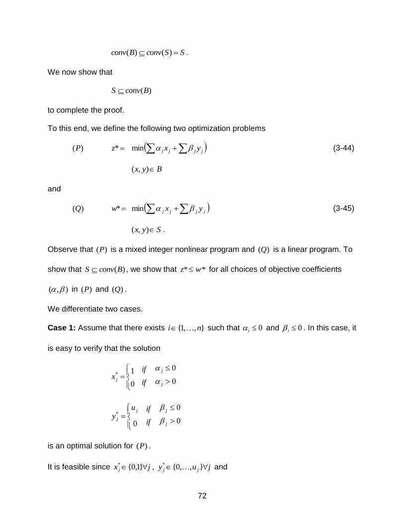
72

SSconvBconv )()( .

We now show that

)(BconvS

to complete the proof.

To this end, we define the following two optimization problems

)(P *z jjjj yx min (3-44)

Byx ),(

and

)(Q *w jjjj yx min (3-45)

Syx ),( .

Observe that )(P is a mixed integer nonlinear program and )(Q is a linear program. To

show that )(BconvS , we show that ** wz for all choices of objective coefficients

),( in )(P and )(Q .

We differentiate two cases.

Case 1: Assume that there exists },,1{ ni such that 0i and 0i . In this case, it

is easy to verify that the solution

00

01*

j

j

jif

ifx

00

0*

j

jj

jif

ifuy

is an optimal solution for )(P .

It is feasible since jx j }1,0{* , juy jj },,0{* and

73

duuyxyx ii

n

j

jj

11

*

1

*

1

** .

It is optimal since is uses only variables with nonpositive objective coefficients.

Therefore, the optimal value of )(P *z is equal to

*z j

j

j

j

j u

jj

00

We next prove that ** wz .

First observe that every feasible solution satisfies

0jx (3-46)

1 jx (3-47)

0jy (3-48)

jj uy . (3-49)

Then define

jI }0j

jI }0j

jJ }0j

jJ }0j .

If we multiply (3-46) by j for all Ij , (3-47) by j for all Ij , (3-48) by j for all

Jj , and (3-48) by j for all Jj and sum the resulting inequalities, we obtain the

valid inequality for S :

*1 1

zuyx j

Jj

j

Ij

j

n

j

n

j

jjjj

. (3-50)

74

Since every feasible solution of )(Q satisfies (3-50), we obtain that

** wz .

Case 2: Assume that for all },,1{ nj either 0j or 0j . In this case, the natural

solution

00

01*

j

j

jif

ifx

00

0*

j

ji

jif

ifuy

is not directly usable since it is not feasible as

0** Nj

jj yx .

It is easy to see that it is sufficient to modify one of the above term ),( **

jj yx in order to

obtain an optimal solution to )(P . The term to modify is clearly the one for which the

change in objective value is smallest.

We define

jI }0,0 jj

jI }0,0 jj

jI }0,0 jj

jI }0,0 jj .

From our assumption in Case 2, ØI .

For Ij the value of )0,0(),( ** jj yx . Making this term feasible would require

changing it to ),1( d resulting in an increase of objective value of jjjj dd .

75

For Ij the value of ),0(),( **

jjj uyx . Making this term feasible would require

changing it to ),1( iu resulting in an increase of objective value of jjj d .

For Ij the value of )0,1(),( ** jj yx . Making this term feasible would require

changing it to ),1( d resulting in an increase of objective value of jjj dd .

Clearly, we want the smallest increase in objective value. This is obtained by finding any

index i as follows:

}{minarg ,,1

jjnj di . (3-51)

An optimal solution to the problem is therefore given by

00

01

j

j

jif

ifx

00

0

j

jj

jif

ifuy

for in \},,1{j , and

1ix

IiorIiifd

Iiifuy

j

i .

The optimal value of )(P is therefore equal to

IiorIiifd

Iiifu

z

jj

jj

iNj

iij

iNj

j

iNj

iiij

iNj

j

0\0\

0\0\

*

.

We next prove that ** wz by considering 3 subcases.

76

Case 2a: Assume that Ii . Since variables can be reordered, we may assume that

ni , },,1{ rI , },,1{ trI , },,1{ ntI and r 21 . We define

},,0{ r such that 1 n .

Because of the definition of ni in (3-51) we have that

dd njj rj ,,1 (3-52)

dnj trj ,,1 (3-53)

dd nj ntj ,,1 . (3-54)

Consider now the following valid inequalities for S

dydxydxn

tj

j

t

rj

j

r

Pj

j

P

j

j 1111

for ,,0P (3-55)

0jx (3-56)

1 jx (3-57)

0jy (3-58)

jj uy . (3-59)

For constraint (3-55) define the following weights:

1 for 0P

PP 1 for 1,,1 P

n for P ,

which are positive because of the definition of and because are sorted. Now, using

these positive weights on (3-55). We obtain

dydxyydx n

n

tj

jn

t

rj

jn

r

j

jn

j

jj

j

jjn

11111

)( . (3-60)

77

Now multiply constraints (3-58) for rj ,,1 with positive weights )( nj and add

to (3-60). Also multiply constraints (3-56) for ,,1j with positive weights

))(( jnj d and add to (3-60) to obtain

dydxyx n

n

tj

jn

t

rj

jn

r

j

jj

j

jj

1111

. (3-61)

Now multiply constraints (3-56) for rj ,,1 with positive weights j and add to (3-

61) to obtain

dydxyx n

n

tj

jn

t

rj

jn

r

j

jj

r

j

jj 1111

. (3-62)

Next multiply constraints (3-56) for trj ,,1 with positive weights )( nj d and

add to (3-62) to obtain

dyyx n

n

tj

jn

r

j

jj

t

j

jj 111

. (3-63)

Then multiply constraints (3-59) for trj ,,1 with positive weights j and add to

(3-63) to obtain

t

rj

jjn

n

tj

jn

t

j

jj

t

j

jj udyyx1111

. (3-64)

Next multiply constraints (3-58) for ntj ,,1 with positive weights )( nj and add

to (3-64) to obtain

t

rj

jjn

n

j

jj

t

j

jj udyx111

. (3-65)

Finally multiply constraints (3-57) for ntj ,,1 with positive weights j and add to

(3-65) to obtain

78

1

1111

n

tj

j

t

rj

jjnn

n

j

jj

n

j

jj udyx . (3-66)

Inequality (3-66) shows that every feasible solution to )(Q satisfies

*11

zyxn

j

jj

n

j

jj

,

i.e.,

** zw .

Case 2b: Assume that Ii . Since variables can be reordered, we may assume that

ti , },,1{ rI , },,1{ trI , },,1{ ntI and r 21 . We define

},,0{ r such that 1 t .

Because of the definition of ti in (3-51) we have that

tjj d rj ,,1 (3-67)

tj trj ,,1 (3-68)

tjd ntj ,,1 . (3-69)

Consider the following valid inequalities for S

dydxdxyn

tj

j

t

rj

j

r

Pj

j

P

j

j 1111

for ,,0P (3-70)

0jx (3-71)

1 jx (3-72)

0jy (3-73)

jj uy . (3-74)


79

1 for 0P

PP 1 for 1,,1 P

t for P ,



dydxdxydx t

n

tj

jt

t

rj

jt

r

j

jt

j

jjt

j

jj

11111

)( . (3-75)

Now multiply constraints (3-71) for tj ,,1 with positive weights dtj )( and

add to (3-75). Also multiply constraints (3-73) for ,,1j with positive weights

))(( jtjd and add to (3-75) to obtain

dydydx t

n

tj

jt

j

jj

t

j

jj

111

, (3-76)

or equivalently,

t

n

tj

jt

j

jj

t

j

jjd

yyx

111

(3-77)

since d is positive.


77) to obtain

t

n

tj

jtr

j

jj

t

j

jjd

yyx

111

. (3-78)

Next multiply constraints (3-74) for trj ,,1 with positive weights j and add to

(3-78) to obtain

80

1

1111

t

rj

jjttt

n

tj

jtt

j

jj

t

j

jj uud

yyx

. (3-79)

Multiply constraints (3-73) for ntj ,,1 with positive weights )(d

tj

and add to (3-

79) to obtain

1

111

t

rj

jjttt

n

j

jj

t

j

jj uuyx . (3-80)


(3-80) to obtain

1

1 111

t

rj

n

tj

jjjttt

n

j

jj

n

j

jj uuyx . (3-81)


*11

zyxn

j

jj

n

j

jj

,

i.e.,

** zw .

Case 2c: Assume that Ii . Since variables can reordered, we may assume that

ri , },,1{ rI , },,1{ trI , },,1{ ntI and 121 r . We define

}1,,0{ r such that 1 ddd rr .

Because of the definition of ri in (3-51) we have that

dd rrjj rj ,,1 (3-82)

drrj trj ,,1 (3-83)

dd rrj ntj ,,1 . (3-84)

81

Consider the following valid inequalities for S

dydxydxn

tj

j

t

rj

j

r

Pj

j

P

j

j 1111

for ,,0P (3-85)

0jx (3-86)

1 jx (3-87)

0jy (3-88)

jj uy . (3-89)


1d for 0P

PP dd 1 for 1,,1 P

dd rr for P ,



r

j

jrr

j

jj

j

jjrr ydyddxdd111

)()(

ddyddxd rr

n

tj

jrr

t

rj

jrr )()()(11

. (3-90)

Now multiply constraints (3-88) for rj ,,1 with positive weights ))(( rrj dd

and add to (3-90). Also multiply constraints (3-86) for ,,1j with positive weights

))()(( rrjj dd and add to (3-90) to obtain

ddyddxdyddx rr

n

tj

jrr

t

rj

jrr

r

j

jj

j

jj )()()(1111

, (3-91)

or equivalently,

82

rr

n

tj

jrr

t

rj

jrr

r

j

jj

j

jj dyd

dxdyx

1111

)()( (3-92)

since d is positive.


92) to obtain

rr

n

tj

jrr

t

rj

jrr

r

j

jj

r

j

jj dyd

dxdyx

1111

)()( . (3-93)

Next multiply constraints (3-86) for trj ,,1 with positive weights ))(( rrj d

and add to (3-93) to obtain

rr

n

tj

jrr

r

j

jj

t

j

jj dyd

dyx

111

)(. (3-94)

Multiply constraints (3-89) for trj ,,1 with positive weights j and add to (3-94)

to obtain

t

rj

jjrr

n

tj

jrr

t

j

jj

t

j

jj udyd

dyx

1111

)(

. (3-95)

Multiply constraints (3-88) for ntj ,,1 with positive weights ))(

(d

d rrj

and

add to (3-95) to obtain

t

rj

jjrr

n

j

jj

t

j

jj udyx111

. (3-96)


(3-96) to obtain

n

tj

j

t

rj

jjrr

n

j

jj

n

j

jj udyx1111

. (3-97)

83


*11

zyxn

j

jj

n

j

jj

,

i.e.,

** zw .

This concludes the proof. ■

Proposition 3.4.3.1 provides a proof of convex hull for integer bilinear covering

sets in case 0. We believe the polyhedral characterization for case 1 given in (3-35) –

(3-41) defines the convex hull for this case also. We do not however have a proof of this

result at this time.

84

CHAPTER 4 SUMMARY

In this thesis, we studied the polyhedral structure of an integer bilinear covering

set which appears in the formulation of several practical problems in optimization

including staff scheduling. During the study, we established that the polyhedral structure

of this covering set depends strongly on some of its parameters

We conjectured polyhedral description of the convex hull for two different cases.

We then investigated these conjectures. In particular, for these two cases, we proved

that several families of inequalities are facet-defining. For one of the cases, we also

showed that these inequalities are sufficient to describe the convex hull.

Proving that the inequalities we derived for case 1 are sufficient to describe the

convex hull in this case is a direct avenue of research in studying these covering sets.

Developing polyhedral descriptions of the convex hull for the remaining cases is another

interesting direction of research. For these other cases we believe it will typically be

hard to uncover a generic form of the convex hull but some families of valid inequalities

might be possible to describe.

85

APPENDIX MATLAB CODES

1. For Case 0, d =3, n = 2

x = [0 0 0 0]

y = [0 0 0 0]

for i = 1 : 63

x(1) = x(1) + 1

j = 1

m = rem(j,2)

while (x(j) > m)

x(j) = 0

x(j+1) = x(j+1) +1

j = j + 1

k = rem(j,2)

if (k == 0)

m = 3;

else

m = 1;

end

end

y=[y;x];

end

x = [1 3 1 3]

86

for i = 1 : 63

if (y(i,1)*y(i,2) + y(i,3)*y(i,4) >=3)

x = [x;y(i,:)]

end

end

2. For Case 0, d =4, n = 2

x = [0 0 0 0]

y = [0 0 0 0]

for i = 1 : 99

x(1) = x(1) + 1

j = 1

m = rem(j,2)

while (x(j) > m)

x(j) = 0

x(j+1) = x(j+1) +1

j = j + 1

k = rem(j,2)

if (k == 0)

m = 4;

else

m = 1;

end

87

end

y=[y;x];

end

x = [1 4 1 4]

for i = 1 : 99

if (y(i,1)*y(i,2) + y(i,3)*y(i,4) >=4)

x = [x;y(i,:)]

end

end

3. For Case 0, d =4, n = 3

x = [0 0 0 0 0 0]

y = [0 0 0 0 0 0]

for i = 1 : 999

x(1) = x(1) + 1

j = 1

m = rem(j,2)

while (x(j) > m)

x(j) = 0

x(j+1) = x(j+1) +1

j = j + 1

k = rem(j,2)

if (k == 0)

88

m = 4;

else

m = 1;

end

end

y=[y;x];

end

x = [1 4 1 4 1 4]

for i = 1 : 999

if (y(i,1)*y(i,2) + y(i,3)*y(i,4) + y(i,5)*y(i,6) >=4)

x = [x;y(i,:)]

end

end

4. For Case 1, d =4, n = 3, u1 = 3

x = [0 0 0 0 0 0]

y = [0 0 0 0 0 0]

for i = 1 : 799

x(1) = x(1) + 1

j = 1

m = rem(j,2)

while (x(j) > m)

x(j) = 0

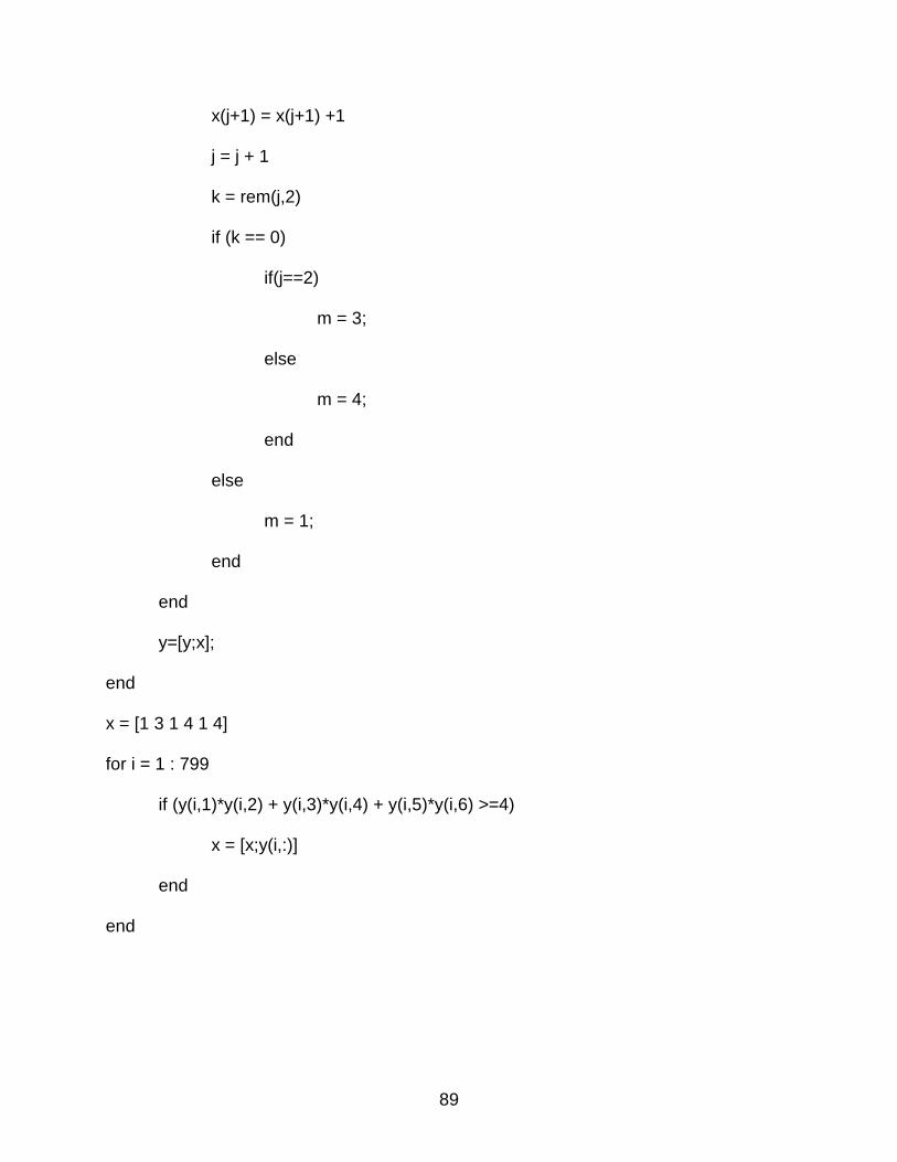
89

x(j+1) = x(j+1) +1

j = j + 1

k = rem(j,2)

if (k == 0)

if(j==2)

m = 3;

else

m = 4;

end

else

m = 1;

end

end

y=[y;x];

end

x = [1 3 1 4 1 4]

for i = 1 : 799

if (y(i,1)*y(i,2) + y(i,3)*y(i,4) + y(i,5)*y(i,6) >=4)

x = [x;y(i,:)]

end

end

90

5. For Case 1, d =4, n = 3, u1 = 2

x = [0 0 0 0 0 0]

y = [0 0 0 0 0 0]

for i = 1 : 599

x(1) = x(1) + 1

j = 1

m = rem(j,2)

while (x(j) > m)

x(j) = 0

x(j+1) = x(j+1) +1

j = j + 1

k = rem(j,2)

if (k == 0)

if(j==2)

m = 2;

else

m = 4;

end

else

m = 1;

end

end

y=[y;x];

end

91

x = [1 2 1 4 1 4]

for i = 1 : 599

if (y(i,1)*y(i,2) + y(i,3)*y(i,4) + y(i,5)*y(i,6) >=4)

x = [x;y(i,:)]

end

end

6. For Case 1, d =5, n = 3, u1 = 4

x = [0 0 0 0 0 0]

y = [0 0 0 0 0 0]

for i = 1 : 1439

x(1) = x(1) + 1

j = 1

m = rem(j,2)

while (x(j) > m)

x(j) = 0

x(j+1) = x(j+1) +1

j = j + 1

k = rem(j,2)

if (k == 0)

if(j==2)

m = 4;

else

92

m = 5;

end

else

m = 1;

end

end

y=[y;x];

end

x = [1 4 1 5 1 5]

for i = 1 : 1439

if (y(i,1)*y(i,2) + y(i,3)*y(i,4) + y(i,5)*y(i,6) >=5)

x = [x;y(i,:)]

end

end

7. For Case 1, d =5, n = 3, u1 = 3

x = [0 0 0 0 0 0]

y = [0 0 0 0 0 0]

for i = 1 : 1151

x(1) = x(1) + 1

j = 1

m = rem(j,2)

while (x(j) > m)

93

x(j) = 0

x(j+1) = x(j+1) +1

j = j + 1

k = rem(j,2)

if (k == 0)

if(j==2)

m = 3;

else

m = 5;

end

else

m = 1;

end

end

y=[y;x];

end

x = [1 3 1 5 1 5]

for i = 1 : 1151

if (y(i,1)*y(i,2) + y(i,3)*y(i,4) + y(i,5)*y(i,6) >=5)

x = [x;y(i,:)]

end

end

94

LIST OF REFERENCES

[1] Al-Khayyal, Faiz A. and Falk, James E. (1983). Jointly Constrained Biconvex Programming. Mathematics of Operations Research 8 273-286.

[2] Balas, E. (1997). Recognizing Facet Defining Inequalities. Acta Mathematica

Vietnamica 22 7-28. [3] Boyd, Stephen and Vandenberghe, Lieven. (2004). Convex Optimization.

Cambridge University Press, New York. [4] Gadsby, G. Neville. (1965). The Army Operational Research Establishment.

Oper. Res. 16 5-18. [5] Hillier, Frederick S. and Lieberman, Gerald J. (2004). Introduction to Operations

Research, eighth edition. McGraw-Hill, Inc., New York. [6] Horst, Reiner and Tuy, Hoang. (1990). Global Optimization. Springer-Verlag,

Berlin. [7] Laderman, Julian D. (1976). A Noncommutative Algorithm for Multiplying 3 x 3

Matrices Using 23 Multiplications. American Mathematical Society 82 126-128. [8] Luenberger, David G. and Ye, Yinyu. (2007). Linear and Nonlinear Programming,

third edition. Springer Science+Business Media, LLC, New York. [9] McCormick, G. P. (1976). Computability of global solutions to factorable

nonconvex programs: Part I. Convex underestimating problems. Mathematical Programming, 10 147--175.

[10] Strassen, Volker. (1969). Gaussian Elimination is not Optimal. Numer. Math, 13

354-356. [11] Tawarmalani, M. and Sahinidis, N. V. (2002). Convexification and Global

Optimization in Continuous and Mixed-Integer Nonlinear Programming. Kluwer Academic Publishers.

[12] Winston, Wayne L. (1995). Introduction to Mathematical Programming, second

edition. Wadsworth Publishing Company, California. [13] Ziegler, Günter M. (1995). Lectures on Polytopes. Springer-Verlag, New York.

95

BIOGRAPHICAL SKETCH

Nitish Garg was born in Hisar, India in 1987. Nitish received a Bachelor of

Technology in Production and Industrial Engineering from Indian Institute of

Technology, Delhi, India in 2009.

Nitish joined the Department of Industrial and Systems Engineering at University

of Florida in August 2009. In summer 2010, Nitish participated in a research project with

Operations Research Group at London School of Economics and Political Science

(LSE) where he worked under guidance of Prof. Gautam Appa. At LSE, his work

involved devising an algorithm to compute Mutually Orthogonal Latin Squares and

implementing it with CPLEX CP Optimizer.

Since August 2010, Nitish has been working with Dr. Jean-Philippe P. Richard.

Upon completion of his master’s degree, Nitish will start working for Bloomberg L.P. as

a Financial Software Engineer. His current interests include mathematics, optimization

and algorithms.

by nitish garg - ufdc image array 2ufdcimages.uflib.ufl.edu/uf/e0/04/29/52/00001/garg_n.pdf · by...

Documents