N C A R Manuscript No. 68-72

Pre-publication review copy

Laboratory investigation of non-steady penetrative convection

By J. W. DEARDORFF, G. E. WILLIS and D. K. LILLY

NATIONAL CENTER FOR ATMOSPHERIC RESEARCH

Boulder, Colorado

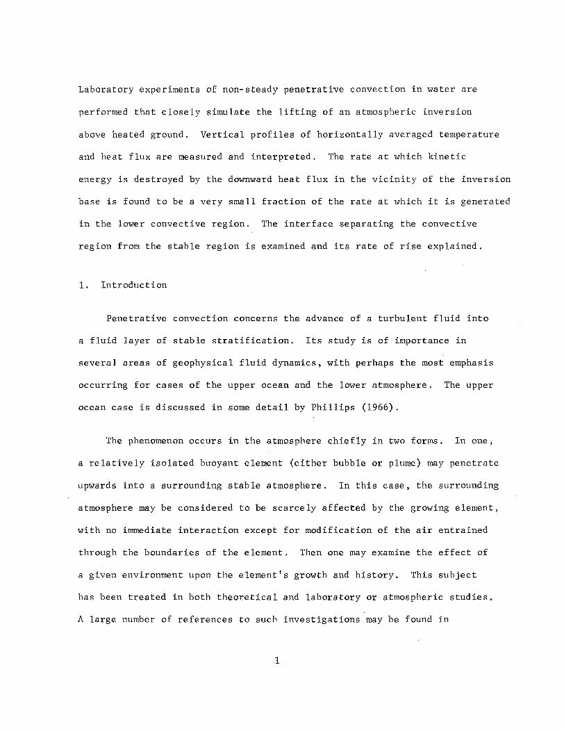
Laboratory experiments of non-steady penetrative convection in water are

performed that closely simulate the lifting of an atmospheric inversion

above heated ground. Vertical profiles of horizontally averaged temperature

and heat flux are measured and interpreted. The rate at which kinetic

energy is destroyed by the downward heat flux in the vicinity of the inversion

base is found to be a very small fraction of the rate at which it is generated

in the lower convective region. The interface separating the convective

region from the stable region is examined and its rate of rise explained.

1. Introduction

Penetrative convection concerns the advance of a turbulent fluid into

a fluid layer of stable stratification. Its study is of importance in

several areas of geophysical fluid dynamics, with perhaps the most emphasis

occurring for cases of the upper ocean and the lower atmosphere. The upper

ocean case is discussed in some detail by Phillips (1966).

The phenomenon occurs in the atmosphere chiefly in two forms. In one,

a relatively isolated buoyant element (either bubble or plume) may penetrate

upwards into a surrounding stable atmosphere. In this case, the surrounding

atmosphere may be considered to be scarcely affected by the growing element,

with no immediate interaction except for modification of the air entrained

through the boundaries of the element. Then one may examine the effect of

a given environment upon the element's growth and history. This subject

has been treated in both theoretical and laboratory or atmospheric studies.

A large number of references to such investigations may be found in

1

Priestley (1959, Ch. 6), with some more recent references in Telford (1967).

In the other form, a turbulent convective fluid covers a large horizontal

area, and may gradually deepen and incorporate a stable fluid layer above it.

This phenomenon is commonly observed when, due to surface heating, a nocturnal

inversion is replaced from below by a growing unstable layer adjacent to the

ground. In this case, the initially stable environment near the ground is

obviously affected by the convection, and full interaction between the two

regions occurs. The convection may still be termed penetrative because the

front of the advancing unstable layer is known to have domes which penetrate

small distances into the stable layer. This form of convection, to be inves-

tigated here, has been the subject of some observational study (Lettau and

Davidson, 1957; Izumi, 1964; Deardorff, 1967; Lenschow and Johnson, 1968),

and of some theoretical modelling (Ball, 1960; Veronis, 1963; Kraus and

Turner, 1967; Lilly, 1968). However, the phenomenon has not received much

detailed laboratory study.

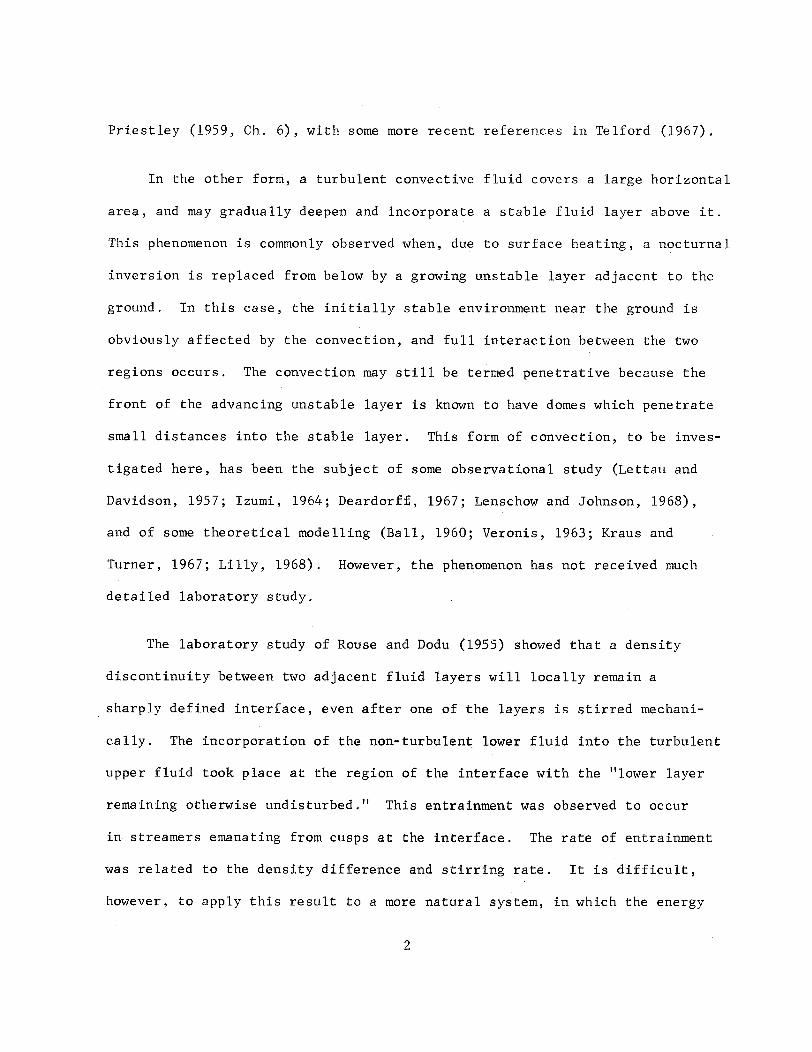
The laboratory study of Rouse and Dodu (1955) showed that a density

discontinuity between two adjacent fluid layers will locally remain a

sharply defined interface, even after one of the layers is stirred mechani-

cally. The incorporation of the non-turbulent lower fluid into the turbulent

upper fluid took place at the region of the interface with the "lower layer

remaining otherwise undisturbed." This entrainment was observed to occur

in streamers emanating from cusps at the interface. The rate of entrainment

was related to the density difference and stirring rate. It is difficult,

however, to apply this result to a more natural system, in which the energy

2

input is by means of a shear stress or heat flux existing throughout a

layer of appreciable depth.

A similar experiment was performed by Cromwell (1960), except that the

stable stratification was associated with a density decreasing continuously

with height over a 15-cm height. As the mixing proceeded, a continuously

sharpening interface did develop, and the entrainment mechanism appears to

have been the same as that described by Rouse and Dodu. The density dif-

ference across the interface increased with time, and was roughly equal to

one-half the product of the initial density gradient and interface depth.

A refinement of Cromwell's experiment was recently performed by Kato

(1967). Mechanical stirring was replaced by application of a constant and

known stress at one boundary. The interface depth was found to be propor-

tional to u, ½ t½, where u, is the friction velocity, the initial

Brunt-Vaisala period, and t is time.

In an experiment by Townsend (1964), a tank of water initially iso-

thermal was cooled from below and heated gently from above. The lower

boundary became cooler than the temperature of maximum density, 4C, so that

an unstable layer developed adjacent to the bottom. As it thickened, a

stable layer developed above it; and, at the end of the experiment, an

equilibrium was approached in which the laminar heat flux directed downward

through the stable layer nearly equalled the value of the downward turbulent

flux below. The experiment disclosed several interesting facts. Except

in the lowest few centimeters, the temperature fluctuations were of maximum

3

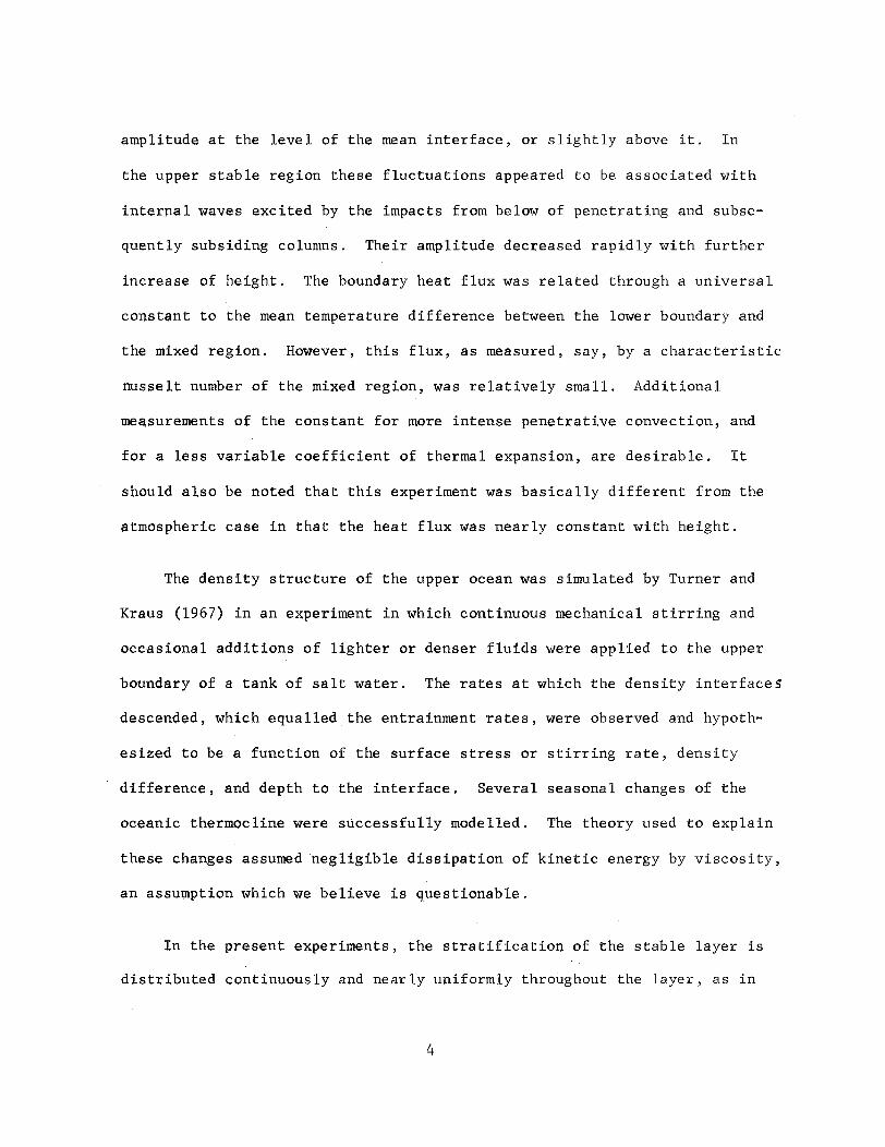
amplitude at the level of the mean interface, or slightly above it. In

the upper stable region these fluctuations appeared to be associated with

internal waves excited by the impacts from below of penetrating and subse-

quently subsiding columns. Their amplitude decreased rapidly with further

increase of height. The boundary heat flux was related through a universal

constant to the mean temperature difference between the lower boundary and

the mixed region. However, this flux, as measured, say, by a characteristic

nusselt number of the mixed region, was relatively small. Additional

measurements of the constant for more intense penetrative convection, and

for a less variable coefficient of thermal expansion, are desirable. It

should also be noted that this experiment was basically different from the

atmospheric case in that the heat flux was nearly constant with height.

The density structure of the upper ocean was simulated by Turner and

Kraus (1967) in an experiment in which continuous mechanical stirring and

occasional additions of lighter or denser fluids were applied to the upper

boundary of a tank of salt water. The rates at which the density interfaces

descended, which equalled the entrainment rates, were observed and hypoth-

esized to be a function of the surface stress or stirring rate, density

difference, and depth to the interface. Several seasonal changes of the

oceanic thermocline were successfully modelled. The theory used to explain

these changes assumed negligible dissipation of kinetic energy by viscosity,

an assumption which we believe is questionable.

In the present experiments, the stratification of the stable layer is

distributed continuously and nearly uniformly throughout the layer, as in

4

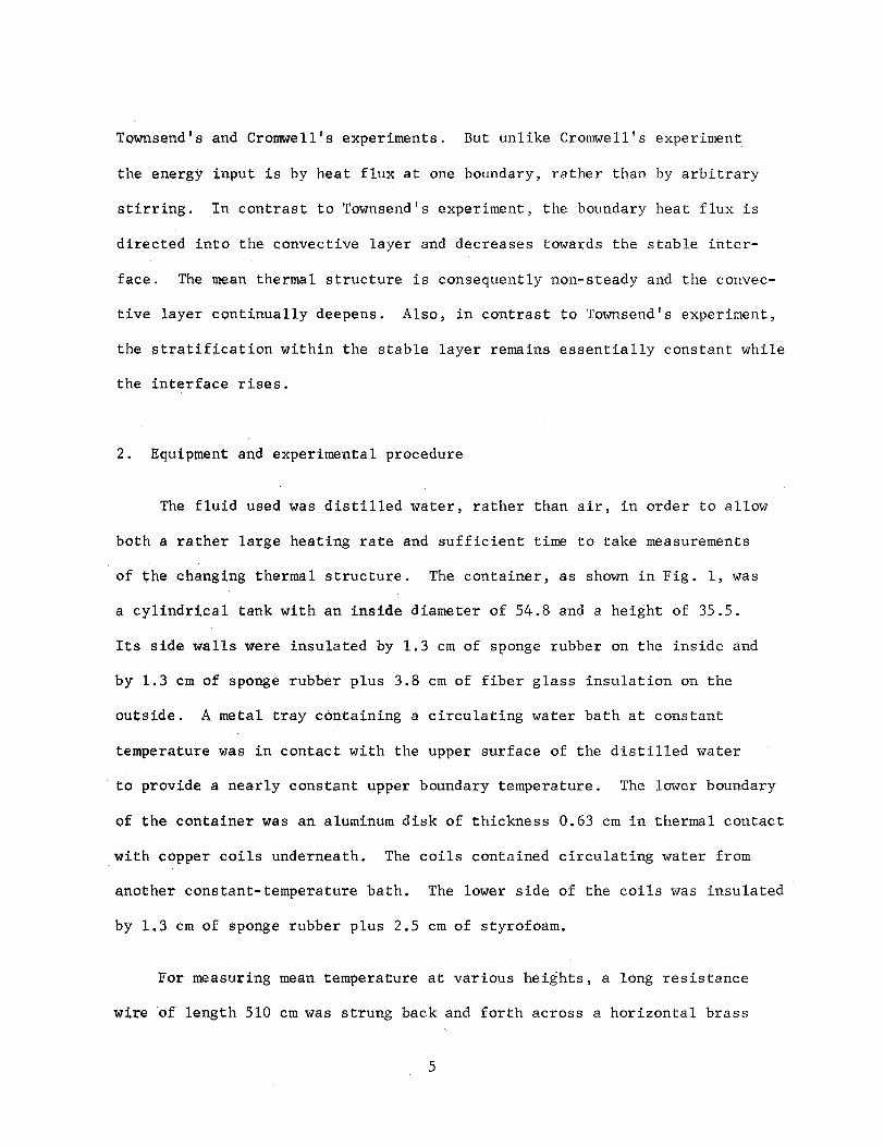
Townsend's and Cromwell's experiments. But unlike Cromwell's experiment

the energy input is by heat flux at one boundary, rather than by arbitrary

stirring. In contrast to Townsend's experiment, the boundary heat flux is

directed into the convective layer and decreases towards the stable inter-

face. The mean thermal structure is consequently non-steady and the convec-

tive layer continually deepens. Also, in contrast to Townsend's experiment,

the stratification within the stable layer remains essentially constant while

the interface rises.

2. Equipment and experimental procedure

The fluid used was distilled water, rather than air, in order to allow

both a rather large heating rate and sufficient time to take measurements

of the changing thermal structure. The container, as shown in Fig. 1, was

a cylindrical tank with an inside diameter of 54.8 and a height of 35.5.

Its side walls were insulated by 1.3 cm of sponge rubber on the inside and

by 1.3 cm of sponge rubber plus 3.8 cm of fiber glass insulation on the

outside, A metal tray containing a circulating water bath at constant

temperature was in contact with the upper surface of the distilled water

to provide a nearly constant upper boundary temperature. The lower boundary

of the container was an aluminum disk of thickness 0.63 cm in thermal contact

with copper coils underneath. The coils contained circulating water from

another constant-temperature bath. The lower side of the coils was insulated

by 1,3 cm of sponge rubber plus 2.5 cm of styrofoam.

For measuring mean temperature at various heights, a long resistance

wire of length 510 cm was strung back and forth across a horizontal brass

5

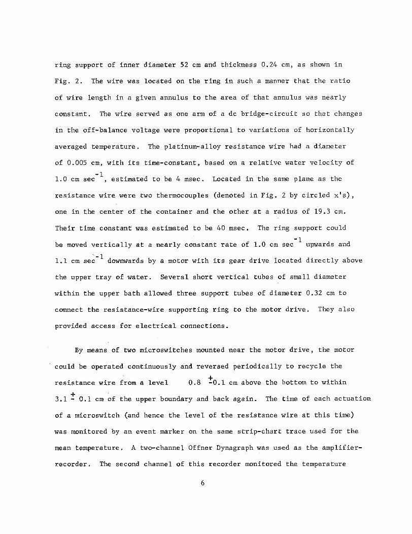
ring support of inner diameter 52 cm and thickness 0.24 cm, as shown in

Fig. 2. The wire was located on the ring in such a manner that the ratio

of wire length in a given annulus to the area of that annulus was nearly

constant. The wire served as one arm of a dc bridge-circuit so that changes

in the off-balance voltage were proportional to variations of horizontally

averaged temperature. The platinum-alloy resistance wire had a diameter

of 0.005 cm, with its time-constant, based on a relative water velocity of

-11.0 cm sec , estimated to be 4 msec. Located in the same plane as the

resistance wire were two thermocouples (denoted in Fig. 2 by circled x's),

one in the center of the container and the other at a radius of 19.3 cm.

Their time constant was estimated to be 40 msec. The ring support could

-lbe moved vertically at a nearly constant rate of 1.0 cm sec upwards and

N-11.1 cm sec downwards by a motor with its gear drive located directly above

the upper tray of water. Several short vertical tubes of small diameter

within the upper bath allowed three support tubes of diameter 0.32 cm to

connect the resistance-wire supporting ring to the motor drive. They also

provided access for electrical connections.

By means of two microswitches mounted near the motor drive, the motor

could be operated continuously and reversed periodically to recycle the

resistance wire from a level 0.8 -0.1 cm above the bottom to within

3.1 - 0.1 cm of the upper boundary and back again. The time of each actuation

of a microswitch (and hence the level of the resistance wire at this time)

was monitored by an event marker on the same strip-chart trace used for the

mean temperature. A two-channel Offner Dynagraph was used as the amplifier-

recorder. The second channel of this recorder monitored the temperature

6

of the lower boundary as sensed by copper-constantan thermocouple in contact

with the bottom aluminum disk. Another dual-channel recorder monitored the

signals of the thermocouples, which moved along with the resistance wire.

The fluid initial conditions were zero velocity and a continuous,

approximately linear temperature-increase with height. At the upper boundary,

z = h, the temperature was maintained at about 39C. At the lower boundary,

three initial temperatures, Tbo, were used as indicated in Table 1. The

continuous initial-temperature condition was attained by filling the tank

slowly at the level of a floating plywood disk with successive increments

of warmer water, and allowing the resulting steps to smooth out over a period

of about 6 hours. This length of time was sufficient to eliminate most of

the curvature in the temperature profile except near the upper boundary,

where some increased stirring occurred as the plywood disk was removed. The

experiments to be presented were terminated before the warming reached this

level.

The thermal convection was initiated at time t = 0 upon replacing the

cool water circulating under the lower boundary with warm water of temperature

greater than the upper boundary temperature. Within 2 minutes the bottom

temperature, Tb, increased rapidly to at least 82% of its final value and

thereafter gradually approached the final value. An average bottom tem-

perature, Tbm, listed in Table 1, was taken as the mean over the time interval

of heat-flux profiles to be presented. The temperature Tb at any time was

not quite uniform horizontally, but generally increased about 0.3C from the

center of the disk to near the outer edge.

7

Table 1

Designation

of experiment

A

B

C

Tbo

0 C)

21.5

29.6

21.3

Tbm

43.4

40.7

39.2

(aT/az)o( C cm )

0.45

0.21

0.47

Time requiredfor h. = 27.5 cm

1

(min)

6.8

7.3

15.2

7A

(sec)

17.4

23.7

16.8

During an experiment the resistance wire was cycled repeatedly to

obtain successive mean temperature profiles. A test was performed to deter-

mine the effect, if any, which movement of the resistance wire and its

supporting ring would have upon the mean temperature structure. Since any

effect would be most serious in the absence of natural motions, the test was

performed while the water was still entirely stratified, with Tb = Tbo. The

resistance wire was cycled 30 times at the same rate as during an experiment,

and the consecutive means profiles obtained differed imperceptibly in shape,

although a slow apparent drift in mean temperature occurred. Any stirring

by the sensor and support should have tended to decrease the temperature

gradient in the region of sensor movement, and increase gradients near the

boundaries. Since this effect was absent, it was concluded that the sensor

and probe movement did not cause any significant mixing of the water. This

result is not unexpected since the average reynolds number of the moving

resistance wire is about 1 and that of the support ring about 35. However,

a significant drift did exist in either the recorder zero-position or the

resistance wire bridge-balance, or both. Hence, in analyzing the experi-

mental observations, corrections were applied to the data to eliminate any

long-term drift by assuming that the mean temperature near the top at

z = 32.4 cm was constant with time. The average temperature correction

between successive profiles was 0.007C.

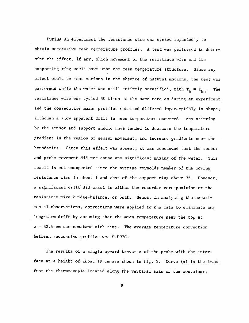
The results of a single upward traverse of the probe with the inter-

face at a height of about 19 cm are shown in Fig. 3. Curve (a) is the trace

from the thermocouple located along the vertical axis of the container;

8

curve (b) is from the thermocouple located at a radius of 19.3 cm; and

curve (c) is that of the resistance wire. Temperature fluctuations of

magnitude 0.5C are present in the thermocouple traces, while fluctuations

of this nature are virtually absent from the resistance wire output due to

the temperature being averaged over the entire length of the resistance wire.

It is evident that mean-value calculations performed from the resistance

wire data are subject to considerably less sampling error than those from

thermocouple data, while the latter more effectively bring out details of

the sharp turbulent interface.

In one series of experiments the resistance wire and several thermo-

couples were maintained at fixed heights throughout the experiment in order

to estimate the temperature variance at these heights. These experiments

were similar to either A or C except that boundary heat fluxes were slightly

smaller.

Some preliminary visual experiments with dyes were performed (in a

rectangular, plexiglass tank with horizontal dimensions 50 x 50 cm and

height 35 cm); and qualitative observations from these experiments will

be introduced in this paper. Essentially, two kinds of dye experiments

were performed, one to view the movement and shape of the interface, the

second to observe the water entraining into the convective layer.

3. Methods of data analysis

Each mean-temperature profile to be presented was first obtained as

9

an average of four consecutive traverses of the resistance wire -- upwards,

downwards, upwards and downwards, in that order. Hence each profile is

centered at the same time at each level, but is an average over about 2 min.

near the bottom and 1 minute near the top. Each profile is furthermore an

average over three experiments, each with nearly the same initial conditions.

Corrections were applied to the original temperatures for instrumental zero-

drifts as previously described.

The heights to which the mean temperatures T apply were obtained from

knowledge of the average resistance-wire height when the event-marker micro-

switches near the terminals of a traverse were tripped, and by assuming a

linear travel speed and recorder chart speed between these points. There

was no indication that these assumptions were in significant error, as the

motor acceleration for each traverse occurred almost entirely before the

initial event-marker microswitch was triggered, and the subsequent decelera-

tion occurred entirely after the final event-marker microswitch was triggered.

Data gathered when the probe speed was not uniform were not used in the

analysis. The height limits used (as measured from the lower boundary)

were 1.3 cm and 32.4 cm.

Mean temperatures were digitized at height intervals of 0.305 cm, with

subsequent vertical averaging giving a height interval of 0.61 cm between

data points of profiles to be presented. Subsequent calculations were

performed by digital computer.

The heat flux H at level z was obtained by numerical integration of

10

the thermal diffusion equation:

hSH H + T d

where ( is the water density and c its specific heat. In actual practice,

level h in (1) was not the upper boundary height, but was the upper limit

of each traverse, 32.4 cm. At this latter level, H was assumed to be due

to molecular transfer. This assumption is not believed to have led to

serious error except after the interface had approached within about 5 cm

of this level. The time derivative in (1) was taken over an interval of

1 min.

Except in the experiments using dye, the interface itself was not

directly observed. Its mean height had to be inferred from either the mean

temperature profile or from the heat flux profile. From measurements to be

presented, we found that some cooling occurs at a given point before the

local interface reaches that point, with maximum cooling coinciding with

the presence of the local interface. Hence a good definition of the mean

interface height is the level of maximum mean cooling. It is easily shown

that this level coincides with the level of maximum downward heat transport.

Since this latter level is quite well defined (see Figs. 7-9), it will be

used here as the definition of the mean interface height.

The data of the experiment with stationary sensors were digitized at

1-sec intervals. After removal of any long-term trend, each computed value

of the temperature variance was taken as the average.of T'2 over a period

of 40 sec, where T' is the fluctuation of T from a mean over this interval.

11

In addition, each value of variance was an average from two thermocouples,

one located on the centerline of the container and the other at a radius

of 21.2 cm.

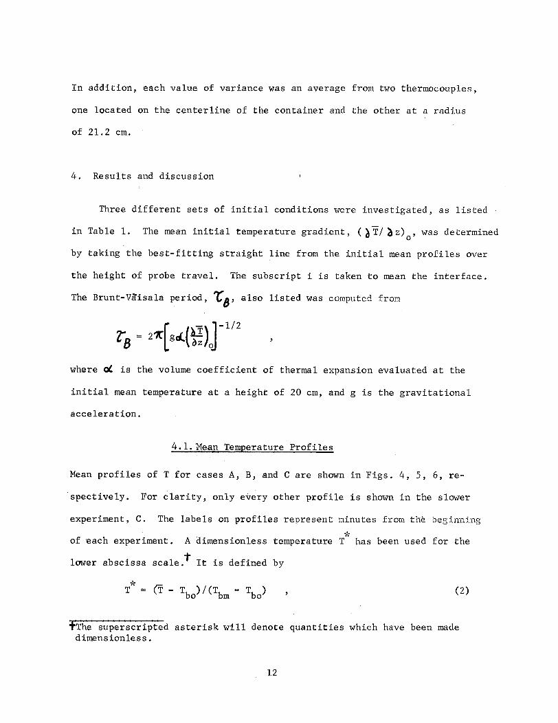
4. Results and discussion

Three different sets of initial conditions were investigated, as listed

in Table 1. The mean initial temperature gradient, ( T/ z) , was determined

by taking the best-fitting straight line from the initial mean profiles over

the height of probe travel. The subscript i is taken to mean the interface.

The Brunt-Va'isala period, 'C, also listed was computed from

S= 290f g(i)] -1/2

where C4 is the volume coefficient of thermal expansion evaluated at the

initial mean temperature at a height of 20 cm, and g is the gravitational

acceleration.

4.1. Mean Temperature Profiles

Mean profiles of T for cases A, B, and C are shown in Figs. 4, 5, 6, re-

spectively. For clarity, only every other profile is shown in the slower

experiment, C. The labels on profiles represent minutes from thL beginning

of each experiment. A dimensionless temperature T has been used for the

lower abscissa scale.t It is defined by

T = CT - Tbo)/(Tbm - Tbo) , (2)

+The superscripted asterisk will denote quantities which have been madedimensionless.

12

where T is the mean temperature (horizontally averaged), Tbo the initial

value of Tb, and Tbm the mean of Tb already defined.

The height scale on the left-hand ordinate is also dimensionless, and

is defined by

z = (Tbm - Tbo) (T/z)o z . (3)

An intense lapse rate (not measured) exists below the lowest level

of measurement, with T = 1 at z = 0. The well-mixed, nearly isothermal

region commences above this level, and increases in depth as the experiment

progresses. The lapse rate becomes slightly stable well before the inversion

base is reached. The pronounced counter-gradient slopes of the first two

profiles after the initial one in each experiment are mostly fictitious and

arise from the use of time averages when the interface was rising rapidly.

However, the counter-gradient slopes of subsequent profiles are definitely

real and extend from a level somewhat below the interface down to z 0.3.

There is no peaked layer of minimum temperature just below the inversion,

as was found by Townsend (1964) when measuring temperatures along a single

column in the center of his convection tank. However, a slight cooling

occurs at a given level just before the interface reaches that level,

especially after the experiment has proceeded several minutes. This cooling

causes the base of the stable layer to be slightly more stable than initially.

An important difference can now be seen to exist between our experiment

and one with mechanical stirring but no heat or mass input. For example,

in Cromwell's experiment (1960), a large density decrease necessarily

13

occurred near the interface level to compensate the equally large increase

near the surface as the mechanical stirring at the top produced a thickening

constant-density layer. The compensation resulted from the absence of any

density sources or sinks. In our experiment, the heat input at the lower

boundary allows the temperature of the well-mixed layer to increase with

very little compensating cooling at the interface level.

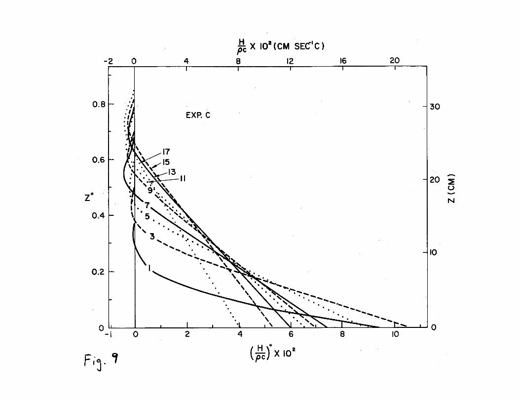
4.2. Heat flux profiles

Corresponding profiles of dimensionless heat flux are presented in Figs.

7, 8, and 9, where successive profiles are drawn with solid, dashed and

dotted lines. The elapsed time for each profile is given in Table 2. The

dimensionless fluxes are defined by

2 1 /3

(H/pc) = (g(Tbm-Tb-4/3 (H/c) , (4)

where K and ) are the thermal diffusivity and kinematic viscosity, respec-

tively, evaluated at the temperature existing at mid-level during initial

conditions.

The reason for making quantities dimensionless in this manner will

be made apparent in section 4.3, although whenever feasible the dimensional

scales are also given on the figures. It may be noticed that (2), (3) and

(4) together indicate that a dimensionless time is correspondingly defined

by

t= ( ) 1(T Tb) t . (5))z o bmbo

14

Table 2

Experiment A

R

0.005

0.020

0.027

0.032

0.023

0.026

C

0.250

0.265

0.238

0.226

0.221

0.214

0.212

Experiment B

Time(min)

0.89

1.86

2.86

3.85

4.84

5.82

6.80

7.80

8.79

R

0.002

0.003

0.010

0.015

0.009

0.005

0.013

0.020

0.018

C

0.219

0.238

0.208

0.205

0.203

0.209

0.195

0.185

0.178

Experiment C

Time(min)

0.96

1.94

2.94

3.93

4.94

5.92

6.90

7.87

8.86

9.85

10.81

11.80

12.80

13.78

14.73

15.71

16.67

17.61

R

0.003

0.002

0.006

0.010

0.010

0.011

0.026

0.017

0.011

0.017

0.019

0.017

0.012

0.026

0.013

0.016

0.038

0.024

14A

Time(min)

0.92

1.89

2.89

3.88

4.85

5.85

6.81

Profile

1

2

3

4

5

6

7

8

9

10

11

12

13

14

15

16

17

18

C

0.250

0.257

0.242

0.227

0.216

0.216

0.199

0.207

0.203

0.207

0.213

0.201

0.213

0.194

0.200

0.186

0.160

0.180

.I i I _ __ I I 1I m -- _-

----- ;,; % 1 I .I . - I - , \ Irl i l l I I

___ _____~ __ I IL -

The heat flux is seen to decrease linearly with height in the lowest

levels, reflecting the fact that the mean temperature profile within the

mixed region retains an almost isothermal shape as warming proceeds.

Generally, the heat flux reverses sign from plus to minus a small distance,

(Az = 0.1), below the mean interface. The negative heat-flux area is

nearly nonexistent early in each experiment, but becomes more pronounced

as the interface rises. (The tiny positive heat flux extending to large

heights for curve 1 in Fig. 7 is probably an error caused by a changing

instrumental drift rate early in that experiment.) The ratio of the area

enclosed by negative heat flux to that of positive flux, R, is tabulated

in Table 2. This ratio signifies what fraction of kinetic energy generated

by buoyancy in the unstable region is being used to increase the potential

energy associated with downward entrainment of the upper warm water, with

consequent lifting of the interface.

It was assumed by Ball (1960) that R = 1, which requires for the atmos-

phere that the rate of viscous dissipation of kinetic energy, 6 , be either

negligible or at most balanced by its rate of production by wind shear. In

our experiment, this assumption would require that 6 at most equal the net

rate of increase of kinetic energy, which was not measured. The very small

values of R in Table 2, with an average magnitude of about 0.015, indicate

only that the net production rate of energy by the heat flux was almost

balanced by the combination of viscous dissipation and kinetic energy increase.

However, the similarity of this type of convection with parallel-plate con-

vection, in which ( generally balances the production by buoyancy, and our

15

order-of-magnitude estimates of kinetic energy increase both indicate that

viscous dissipation was the more important factor here, which counter-

balanced the energy production by buoyancy. The assumption by Turner and

Kraus (1967) that 6 was a negligible item in the energy budget of their

experiment thus appears questionable.

The fact that the negative areas increase with time in each of our

experiments apparently indicates that the viscous dissipation becomes

slightly less efficient in balancing the energy production as the scale of

the motions increases. Any extrapolation of these results to the lower

atmosphere would be highly speculative, however. In studies based upon

a few temperature soundings, a ratio of 0.06 was obtained by Deardorff

(1967, Fig. 4) for the case of cold air flowing from the eastern U. S.

towards Bermuda, while a ratio of 0.4 was obtained by Lenschow and Johnson

(1968, Fig. 8) for the diurnal heating above a Wisconsin forest. These

ratios are highly uncertain because of unknown magnitudes of horizontal

and vertical advection, and direct atmospheric measurements of heat flux

are desirable.

If the area of negative heat flux is assumed to maintain a constant

shape over short time periods as the interface rises, a simple expression

relating the net cooling at the interface to its rate of rise may be

obtained. In this case the mean thermal diffusion equation is

where h. is the mean interface height. If gh./it is relatively much more

16

constant than H/pc above the interface, then the integral of (6) at any

level with respect to time, from an early time until the interface reaches

that level, is

T. (0) - T. (t) - , (7)1 1 c)1 t

where T. (t) is the mean temperature at the interface height, and T. (0)1 1

is the initial mean temperature at the same height. Both sides of (7) have

been plotted against t , and smoothed values from the right-hand side subse-

quently plotted in Fig. 10 against smoothed values from the left for the

same t . Although qualitatively correct, expression (7), given by the solid

line, underestimates the interface cooling by about 40%. Moreover, the

underestimate is made worse if account is taken of the suppression of -(H/ec)

caused by the one-minute time interval over which each heat flux curve was

obtained and by time-smoothing of T profiles. From numerical tests with

model profiles, we believe the suppression to be at the 50% level for profile

number 3 of Fig. 7, but less for subsequent profiles and for experiment C.

(Similarly, the ratio R was found to be underestimated, but by only 15% and

less.) The reason for the theoretical underestimate must reside in the

changing shape of the negative H-region with time.

The right-hand side of (7) has been presented by Ball (1960) as an

expression for the interface temperature discontinuity, rather than for

the maximum mean cooling which occurs at z = h.. This interpretation will

be discussed in section 4.4.

17

4.3 Interface height as a function of time

The mean interface height, h., may be predicted as a function of time,

knowing the initial lapse rate, (2 T/dz) , and the temperature difference

between the heated lower boundary and its initial value, Tbm- Tbo. If

the mixed region is approximated by a single isotherm (or adiabat), and the

slight cooling above the inversion base is ignored, the rise rate is given by

=h _ (.m (8)t tt z) Jo

where T is the temperature of the mixed or turbulent region. The integral

of (8) over time is

h. = (Tm - T ) ) , (9)1 m bo/ )z )osince T = T , initially as a mixed layer starts to develop near the bottom.

m bo

Another relationship for h. comes from the thermal equation, when the

heat flux is assumed to decrease linearly with height from the surface to h.:I

= (H/oc)b /. , (10)

where the small negative heat flux at z - h. has also been ignored.1

If the boundary flux were constant, )T /mt could be eliminated between

(8) and (10) and the result immediately integrated to give

KH/C) 1/2 1/2h (H/ c) (

OL

18

This t 2 dependence is the same as that found by Kato (1967) when the energy

input was by a constant stress at the boundary rather than by applied heat.

Kato found that

(- 1/ 4 1/2h. = 1.9 u - • 1/4(t - t 1/2) , (12)i ( z to 02)

where t is a small virtual displacement of the time origin. If the friction

velocity, u., in (12) were replaced by a thermal convection velocity, w.,

given by

= [goL( o]-1/4 /2

then (12) would be identical to (11) except for the different value of the

constant of proportionality. Unfortunately there appears to be no simple

means of deducing the value of the constant in (12) as there is for (11).

In our study, the lower boundary temperature was more constant than

the boundary heat flux. The latter can be related to T - T by Townsend'sSbm m

(1964) dimensional argument,

1/3 4/3

)b = ( g4) (Tbm - Tm) (13)

where C is a universal constant (see 4.6).

If (H/pc)b and h. are eliminated between (9), (10) and (13), the

resulting equation for T (t) is

m

1/3

(-m -Tbo)4/3 = C g ~) . (14)(Tbm - Tm)4 ! 3 t

19

Upon rearrangement, (14) may be written

F-1/3 -4/3 (Tb -T)- (Tb - T ) + (T - Tbo) (Tbm Tm ) b m -bm m bm bo bm m It

=C- g g o . (15)(( )1Integration of (15) then gives

1 * 2/3 2 1/3 2 *31- T + 1- T = 1 + Ct , (16)

where T is the dimensionless temperature defined in (2) and applied tom

the mixed region, and t is the dimensionless time defined in (5). In (16)

the initial condition T = Tb has again been used.mo bo

From (2) and (9) it is also seen that

h. = T . (17)1 m

Elimination of T between (16) and (17) gives h. as a function of t , whichm 1

is shown in Fig. 11 by the solid curve, computed for C = 0.21, an average

value obtained for this constant. The data points give the observed inter-

face heights, h. , as a function of t . The theoretical underestimation1

of h. by about 10% is associated with its underestimation by (9), due at1

first to the assumption of isothermal profiles instead of the actual counter-

gradient profiles, and due later also to the neglect of the interface cooling.

If experimental values of Tm (see (17)) were plotted in Fig. 11, they

would lie closer to the theoretical curve.

20

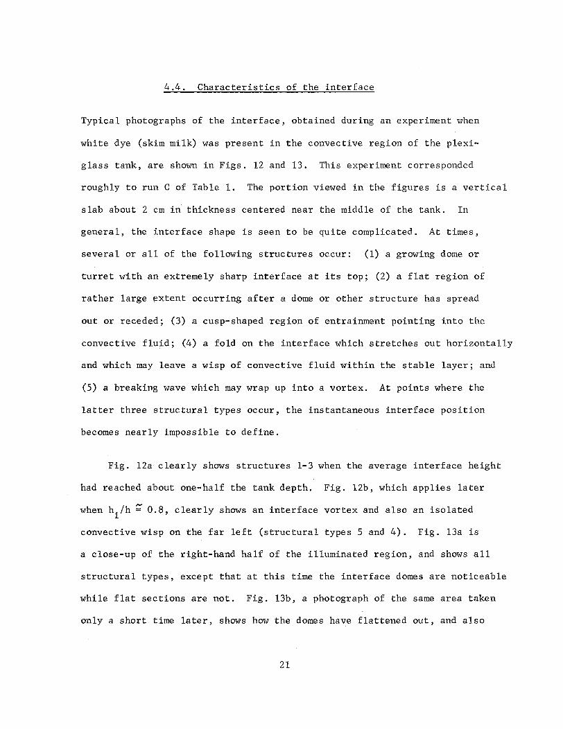
4.4. Characteristics of the interface

Typical photographs of the interface, obtained during an experiment when

white dye (skim milk) was present in the convective region of the plexi-

glass tank, are shown in Figs. 12 and 13. This experiment corresponded

roughly to run C of Table 1. The portion viewed in the figures is a vertical

slab about 2 cm in thickness centered near the middle of the tank. In

general, the interface shape is seen to be quite complicated. At times,

several or all of the following structures occur: (1) a growing dome or

turret with an extremely sharp interface at its top; (2) a flat region of

rather large extent occurring after a dome or other structure has spread

out or receded; (3) a cusp-shaped region of entrainment pointing into the

convective fluid; (4) a fold on the interface which stretches out horizontally

and which may leave a wisp of convective fluid within the stable layer; and

(5) a breaking wave which may wrap up into a vortex. At points where the

latter three structural types occur, the instantaneous interface position

becomes nearly impossible to define.

Fig. 12a clearly shows structures 1-3 when the average interface height

had reached about one-half the tank depth. Fig. 12b, which applies later

when h./h = 0.8, clearly shows an interface vortex and also an isolated1

convective wisp on the far left (structural types 5 and 4). Fig. 13a is

a close-up of the right-hand half of the illuminated region, and shows all

structural types, except that at this time the interface domes are noticeable

while flat sections are not. Fig. 13b, a photograph of the same area taken

only a short time later, shows how the domes have flattened out, and also

21

reveals an additional vortex at the upper left edge of the main entrainment

region. From the point of view of the Helmholtz instability criterion, the

appearance of breaking waves is not surprising. Neglecting the effect of

-lviscosity, interface velocity differences of magnitude 0.5 cm sec are

sufficient to give instability to waves of length 5 cm and less.

As a result of these interesting structures the instantaneous interface

in our experiments was not apparently as sharp as that reported by Rouse

and Dodu (1955), who used fluids of two different densities. Even in our

study, however, the interface tended to be rather well defined despite the

occasional ejection of convective fluid into the base of the stable region.

There are two reasons for this. First, penetration in the form of domes

cannot eject convective fluid into the stable region because the restoring

force of buoyancy eventually causes the fluid within the dome to recede.

Yet, growing and receding domes occupy a substantial portion of the interface.

Secondly, convective fluid which does get stranded by a folding of the inter-

face can be deposited only a short distance above the interface. Before

long it is entrained downwards adjacent to a dome-shaped structure, leaving

only original stable fluid adjacent to the dome. The entraining fluid, of

course, is not subject to a strong restoring force once it has moved into

the more uniform convective region, and it is very unlikely ever to return

to the stable region.

Visual observations taken when blue dye was in the stable layer

generally confirmed the observations of Rouse and Dodu that entrainment

22

occurs as wisps streaming down from cusps adjacent to domes. The streamers

typically had a maximum width of only 2 or 3 cm near the interface, tapering

to a few millimeters well below the interface. Many of them descended to

the bottom, moved horizontally, and then moved upwards again before dis-

appearing from view. This complete mixing was also observed by Townsend

(1964), From these observations, velocities within the convective region

-lfor run C are estimated to have been 2 cm sec1 and less.

Although maximum entrainment occurred at edges of rapidly growing

domes, streamers were most prevalent in the central region of the tank.

This result is associated with a general circulation of rising water near

the corners and walls, with sinking motion in the center. A net circulation

of this type seems to be typical of fluids heated from below and confined

on the sides (Townsend, 1959), and not a result of slight inequalities of

surface temperature.

The local temperature structure at the interface was inferred from

traces of thermocouples attached to the moving resistance-wire frame.

Typical vertical traces from upward traverses of experiment A are shown

in Fig. 3. In profile (b) a steep gradient at the local interface is

especially evident. Sometimes no such interface was evident, from which

it is surmised that the thermocouple passed through a region of entrainment.

Where present, the interface discontinuity,AT., was typically of magnitude

0.5C. Because of the continual heating from below,- T. did not increase

in proportion to hi, as would the density discontinuity in an experiment

of the kind performed by Cromwell (1960) or Kato (1967).

23

In the penetrative convection models used by Ball (1960) and Lilly

(1968), the interface irregularities were assumed to be extremely small

compared to the mean interface height. The average cooling of equation

(7) or Fig. 10, which had occurred at a given level by the time the mean

interface reached that level, then would become synonomous with the tem-

perature discontinuity across the interface, AT.. Hence their models

predicted that

AT= - (H/c)i/ (18)

for the case of no subsidence and no radiative or evaporative cooling.

Our measured values of ATi ranged systematically from 1 to 5 times

larger than the right-hand side of (18), except towards the end of experi-

ment C, when they became smaller. Most of the theoretical underestimate

can probably be attributed to the fact that the interface irregularities

are not negligibly small, and that the horizontally averaged temperature

profile is quite different from an individual temperature sounding. A

small part of the discrepancy can be attributed to the experimental under-

estimate early in the experiments of -H. (discussed in section 4.2).1

Townsend (1964) noted that the temperature fluctuations have a maximum

amplitude near the bottom of the stable region. We observe the same result

in Figs. 14 and 15, where the root-mean-square temperature fluctuation is

given as a function of time for experiments A and C, respectively. The

data points were obtained as described in section 3 from fixed thermocouples

at two different levels, and in these two figures the overbar represents

a time average. The arrows denote our estimates of the time of passage

24

of the mean interface level, taken here to be the time of occurrence of

lowest temperature on each thermocouple trace. The maximum intensity

appears to occur slightly above the interface level (before interface

passage) simply because diffusive mixing, which helps smooth out the

fluctuations, is present below the interface and nearly absent above. In

each figure, the maximum intensity occurs at the greater height in spite

of the fact that the surface heat flux is then somewhat smaller. Only in

experiment A is the maximum dimensional rms fluctuation at the upper level

as large as the maximum observed by Townsend (1964) upon dividing his

peak-to-peak values by 6 for comparison purposes.

From Fig. 14 we may obtain an estimate of the maximum vertical extent

of the interface waviness or irregularity. A formula valid for internal

waves is

= - T , (19)

where is the vertical displacement of a particle from its initial position

at rest, and T' is its associated temperature fluctuation. Applying the

square of (19) to particles initially at the level of the interface when

the latter has reached a height of, say, 25 cm, averaging horizontally and

taking the square root, we obtain

( )1/2 1/2(=T / o.z =0 0.7 cm, (20)

for experiment A. The peak displacement can be expected to have an amplitude

three times this, and the maximum peak-to-trough extent is expected to be

25

another factor-of-two larger, or about 4 cm. Although this estimate

incorporates several uncertainties, it agrees rather well with estimates

from our visual observations. These, however, corresponded more closely

with experiment C than with A. Visual estimates of the vertical extent

of the interface are themselves highly uncertain because the lower inter-

face limit estimated for regions of entrainment is an arbitrary matter.

If the value of 4 cm is centered at the interface level of curve 5 in

Fig. 7, most of the region of negative heat flux falls within this interval.

The inference to be drawn is that the entrainment process, which requires

a contorted interface for its existence, can probably explain all but a

small "tail" (at higher levels)of the negative heat flux observed.

4.5 The stable region

Temperature measurements from fixed thermocouples well within the stable

region showed rather regular oscillations having the appearance of internal

gravity waves. A typical record at height 29.1 cm for experiment A is

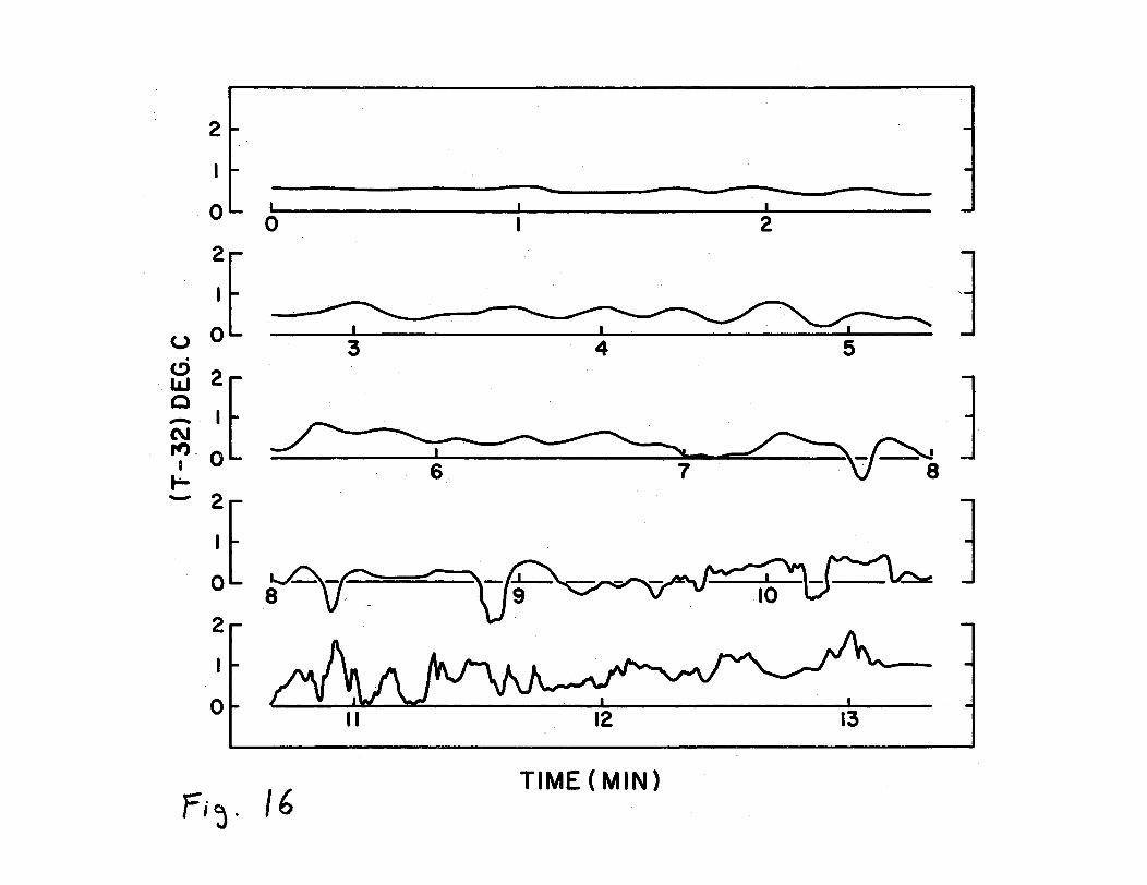
shown in Fig. 16. As noticed by Townsend (1964) the wave-induced fluctua-

tions well above the interface are not skewed or asymmetric as they are

in much of the convective region. However, at times 7.7, 8.2, and 8.9 min

asymetric cold peaks occur. These must have been associated with the

close approach from below of relatively cold interface domes which subse-

quently receded. At 8.9 min an interface dome appears to have moved

slightly above the thermocouple for a few seconds. (Presence of the con-

vective region is inferred from relatively high frequency fluctuations

indicative of small-scale motions and significant molecular smoothing.)

26

After abour 9.2 min the interface appears to have passed and to have

remained above the thermocouple except perhaps for brief retrogressions

centered at 10.0 and 10.6 min. Between 11 and 12 min, some reverse

asymmetry is present, and is probably associated with narrow streamers

of warm fluid entraining downwards. A net cooling at the thermocouple

preceding the interface passage is evident between about 6.7 and 9.2 min.

The initial period of the internal waves is seen to be about 25 sec

in Fig. 16. This period is considerably longer than the Brunt-VSisala

period of 17.4 sec, listed in Table 1. Longer periods are theoretically

expected to be associated with waves whose vertical structure is sinusoidal

in character, with a nodal plane at the upper boundary (Phillips, 1966,

p. 164). Shorter periods are associated with waves which decay with height

nearly exponentially at a rate proportional to the difference between the

Brunt-Vaisala period and the actual enforced period. Hence, the convec-

tively forced waves of short period cannot become evident until the inter-

face is relatively close to the thermocouple. This qualitative behavior

is apparent in Fig. 16, although a rigorous analysis of the internal wave

motion should allow for the fact that the coefficient of thermal expansion

of water varies considerably with temperature, even at temperatures well

above 4C.

The intensity of the temperature fluctuations induced by internal

waves shows an interesting difference in Figs. 14 and 15. In the former

case (experiment A), in which the interface rose quite rapidly, significant

fluctuations first occurred at about the same time at both heights

27

of measurement, and increased initially at about the same rate. In Fig. 15

(experiment C), associated with a more slowly rising interface, the fluc-

tuations occurred earlier at the lower level and increased much more rapidly

there, until interface passage, than at the higher level. This latter

behavior means that T' 2 decreased rapidly with height well above the inter-

face level, in agreement with Townsend's (1964) steady-state data. On the

other hand, the more uniform vertical distribution of T'2 of our experiment

A, well above the interface, implies a greater relative amplitude of internal

waves with sinusoidal-type vertical dependence in this case. This in turn

implies a frequency spectrum of vertical velocities in the convective region

having greater intensity at lower frequencies than in experiment C. This

conclusion is plausible in view of the greater heat flux in experiment A

than in C.

The net cooling at a point above the interface in Fig. 16, and the

small tails to the negative heat flux curves of Figs. 7-9, which apparently

extend above the highest level reached by any portion of the local inter-

face, require some discussion. (The tails probably were suppressed late

in each experiment by our assumption of constant mean temperature at

z = 32.4 cm.) In the absence of any evident small-scale mixing or wave-

breaking this far above the interface, it might be thought that internal

gravity waves should not have been responsible. However, inspection of

the thermal-variance equation

S + w'T' + = 0 (21)

28

as applied to the horizontally homogeneous case with negligible thermal

diffusion indicates that a heat transport by (finite-amplitude) internal

waves could be supported by non-steady conditions and/or by vertical

divergence of wT' /2. The non-steady term in (21) is of the proper sign

to support a negative heat flux above the interface where T'2 increases

with time. Since the rate of increase is largest close to the interface,

the vertical divergence of the associated flux would furthermore produce a

cooling as observed. However, the magnitude of- , which can be

obtained from Fig. 14, was found to be nearly an order of magnitude too

small to produce the magnitude of negative flux observed in the tails.

Hence the triple-correlation term, , wT'2/2), is probably responsible,

but no convincing explanation for its sign or magnitude is available. The

quantity wT' evidently is negative near the interface and approaches zero

with increasing height.

Two other possible explanations for the cooling and small negative

heat flux in this region were considered but rejected from order-of-magnitude

arguments. First, descending motion adjacent to the imperfectly insulated

walls may have resulted in a slight upward transport within the main body

of fluid covered by the resistance wire. Second, a bulk rising motion of

the slowly warming and expanding water in the convective region may have

caused the water above to lift slightly with respect to a reference height

of the resistance wire, and thus advected cooler water upwards. Both

effects, though undoubtedly present, seem to have been entirely insignificant.

29

4.6. Boundary heat flux

It is of interest to compare Townsend's value of C in (13), obtained for

statistically steady thermal convection of air in an open box, with the

values from our non-steady experiment using water in an enclosed tank. The

temperature of the mixed region, T in (13), was taken to be the lowestm

existing mean temperature. Actual values of Tb were used, rather than values

of Tbm. The quantities K, ), and Otwere evaluated at a temperature midway

between that of the lower boundary and that of the mixed region, and (H/p c)

was taken from Figs. 7-9. Resulting values of C are shown in Table 2.

There is a definite trend toward lower values with increasing time, even

if the first three values in each experiment are rejected on the grounds

of too much time-smoothing of T profiles. We have no explanation for this

trend, but note that values near the ends of the experiments, when conditions

were most steady, lie between 0.18 and 0.21. The average of these agrees

well with the value 0.193 found by Townsend, but perhaps only coincidentally.

If we had evaluated yand C. at the boundary temperature, our C values would

be about 7% smaller.

It might be noted that (13) may not hold well for prandtl numbers

differing strongly from unity. the 1/3-dependence of K 2/%stems from the

observation that the nusselt number in parallel-plate convection is dependent

upon the 1/3-power of the rayleigh number and the assumption that it is

independent of prandtl number. This assumption is not quite correct according

to the weak effect of prandtl number which has been measured by Globe and

Dropkin (1958). The prandtl number in the present experiments ranged from

about 7 at cooler temperatures to about 4 at the highest temperature; in

Townsend's open-box experiment it was 0.7.

30

5. Summary and conclusions

Laboratory experiments of non-steady penetrative convection in water

were performed which closely simulate, except for scale, the lifting of

an atmospheric inversion above heated ground. The horizontally averaged

temperature was found to vary smoothly with height and to undergo a slight

cooling just above the inversion base. The maximum cooling was related to

the downward heat transport at the inversion base and to the rise rate of

the latter. The vertically integrated negative heat flux near the inversion

base was only about 1.5% of the vertically integrated upward flux below.

The local interface between the stable region and the convective region

stayed rather well defined throughout the experiments. The interface shape

is a combination of forms: domes with adjacent cusps through which downward

entrainment occurs, flat sections, folded structures and breaking waves.

The height of the mean level of the interface was quantitatively related to

the boundary heat flux, the lapse rate in the stable region, and the

elapsed time.

Values of the universal constant which relates the boundary heat flux

to the temperature difference between the boundary and the well-mixed region

support the value found earlier by Townsend.

31

REFERENCE S

BALL, F. K. 1960 Control of inversion height by surface heating. Quart.

J. Roy. Meteor. Soc. 86, 483-494.

CROMWELL, T. 1960 Pycnoclines created by mixing in an aquarium tank.

J. Mar. Res. 18, 73-82.

DEARDORFF, J. W. 1967 Empirical dependence of the eddy coefficient for

heat upon stability above the lowest 50 m. J. Appi. Meteor. 6, 631-643.

GLOBE, S. & DROPKIN, D. 1958 Natural convection heat transfer in liquids

confined by two horizontal plates and heated from below, 1958 HeatTransfer and Fluid Mechanics Inst. Berkeley: Univ. of Calif., 156-165.

IZUMI, T. 1964 Evolution of temperature and velocity profiles during

breakdowns of a nocturnal inversion and a low level jet. J. Appl.

Meteor. 3, 70-82.

KATO, H. 1967 On the penetration of a turbulent layer into stratified

fluid, The Johns Hopkins Gravitohydrodynamics Laboratory Rept. No. 2,October 1967. Baltimore, Maryland.

KRAUS, E. B. & TURNER, J. S. 1967 A one-dimensional model of the seasonal

thermocline, Part II. The general theory and its consequences, Tellus

19, 98-106.

LENSCHOW, D. H. & JOHNSON, W. B. 1968 Concurrent airplane and balloon

measurements of atmospheric boundary-layer structure over a forest.

J. Appl. Meteor. 7, 79-89.

LETTAU, H. H. & DAVIDSON, B. 1957 Exploring the Atmosphere's First Mile,

Vols. 1 and 2. New York: Pergamon Press.

LILLY, D. K. 1968 Models of cloud-topped convection layer under a strong

inversion (to be published in Quart. J. Roy. Meteor. Soc.).

PHILLIPS, O. M. 1966 The Dynamics of the Upper Ocean. Cambridge University

Press.

32

References - Continued

PRIESTLEY, C. H. B. 1959 Turbulent Transfer in the Lower Atmosphere. Chicago:

University of Chicago Press.

ROUSE, H. & DODU J. 1955 Turbulent diffusion across a density discontinuity.

La Houille Blanche No. 4, 522-532.

TELFORD, J. W. 1967 The convective mechanism in clear air. J. Atmos. Sci.

23, 652-666.

TOWNSEND, A. A. 1959 Temperature fluctuations over a heated horizontal

surface. J. Fluid Mech. 5, 209-241.

TOWNSEND, A. A. 1964 Natural convection in water over an ice surface.

Quart. J. Roy. Meteor. Soc. 90, 248-259.

TURNER, J. S. & KRAUS, E. B. 1967 A one-dimensional model of the seasonal

thermocline, Part I. A laboratory experiment and its interpretation.

Tellus 19, 88-97.

VERONIS, G. 1963 Penetrative convection. Astrophys. J. 137, 641-663.

33

FIGURE CAPTIONS

Fig. 1. The penetrative-convection container with circulating warm water

in a metal tray on top, and circulating cool or warm water in

coils underneath.

Fig. 2. The vertically moving probe, with resistance wire and two

thermocouples.

Fig. 3. Typical vertical profiles of temperature from two thermocouples,

(a) and (b), and from the resistance wire, (c), during an upward

traverse of experiment A.

Fig. 4. Vertical profiles of horizontally averaged temperature for experi-

ment A. Profile labels give time in minutes. Dimensionless scales

are on bottom and left, dimensional scales on top and right.

Fig. 5. Same as Fig. 4, but for experiment B.

Fig. 6. Same as Fig. 4, but for experiment C.

Fig. 7. Vertical profiles of heat flux for experiment A, with labels giving

time in minutes. Dimensionless scales are on bottom and left,

dimensional scales on top and right.

Fig. 8. Same as Fig. 7, but for experiment B.

Fig. 9. Same as Fig. 7, but for experiment C.

Fig. 10. A theoretical estimate (solid line) of the total mean cooling at the

level and time of mean interface passage versus the observed mean

cooling (data points).

34

Fig. 11. The dimensionless height of the interface, hi., as a function

of dimensionless time, t*. The solid theoretical curve is

from equations (16) and (17).

Fig. 12. Photographs of the convective region and interface within the

tank of width 50 cm and height 35 cm, with conditions similar

to those of experiment C.

(a) Mean interface height about 17 cm.

(b) Mean interface height about 28 cm.

Fig. 12. Close-up photographs of the convective region and interface

during the same experiment as in Fig. 12.

(a) Interface domes sharply outlined.

(b) Interface more diffuse.

Fig. 12. Experimental values of the standard deviation of temperature

(with respect to time-averaging) as a function of time at two

different locations for experiment A. Dimensionless scales

are on bottom and left, dimensional scales on top and right.

Fig. 15. Same as Fig. 14, but for experiment C.

Fig. 16. A record of thermocouple temperature versus time at a height of

29 cm (experiment A).

35

0 ** * S S 0 0 * 00 * 0 0 0 @5

00 *0 5 * * * * * * 0* 0 Os * 0* 0

* * *o *0*e * ** 0

* 0 0 0 * * ** *. 0 * S *.S 0

0 * 0 * * * * * * 0 *

* 0 00s, * . *

0 * * 0S * 0

0 * ** * *0 * * 0 0

0 * * 0 * 6 ** 0

S * 0 0 @0

SYMBOLS: 2ALUMINUM

I'c.

SPONGERUBBER

Io o1

COPPERCOILS

FIBERGLASS

I

EI WATERbp , !pI 10 .0

WATER

- • '• . •

/.~~o •• * * 0 •* * 0

STYRO-FOAM

_i 1 -. v vl .o v -OP w .&K.d . .o . . . .- . ..l'f, .ý .& ,dgKp' • dP" I •pO s,.-0 -01 Jvl gr . . . . .&- . . . M

WATER

THERMOCOUPLES

59.2

DCCI -A TA .Ir-

SS

(b)

024 68 02 46 8

(T-29) DEG.C

F;i. 3

02468

30

2 20

N

10

A\

(a) (c)

T(DEG.C)24 28 32 36

I 1 I I I -

0.6

0.4

0.2

0

30

20 .

N

10

jo0 0.2 0.4 0.6 0.8

4-

/ I I p I I I

T(DEG.C)30 32 34 36

EXP. B

0~ 0.2 0.40.

0.6

0.4

0.2

0

30

20 -20

N

10

0

_ II ' I I I ' I

-

-

I I I I0.20. 0.60

157·

(DEG.C)32

EXP. C

I I

IL0

S I I I I

30

20N)N

0.8

0.6

0.4

0.2

.6

24T

28 36

10

n0 0.2 0.4 0.6 0.8

nI.0

I I L - I -- -

1 II I -- I I i' ' - 1 · II I- -II I I I I I I

-

-

-

I00L

I

H 2 IPC x10 (CM SEC C)

S2 4 6 8 10 12 14

(H)* 02

Fl .7

0.6

Z*0.4

0.2

0

6

30

20 -N

10

n

-a

HPE

2 4

X 2CM SECCXIO ( CMSEC C )

6 8

0 2 4 6 8 10 12

(P) x I2

-I 0 10 12 14

0.6

0.4

0.2

0

30

20

10

0

-X 10 (CM SEC"'C)

2 4 6 8 10

(H x102PC)'x,

0.E

0.6

Z*

0.4

0.2

r

30

20

10

00I O 0

v -

F;g· 9

C 40X*

Ito

eIQ2

A

0 I 2 3

[T* (0) -T*(t)xo 102

Fi. 10

As

0.8

0.6

0.4

0.2

0I 2 3

1*

1.0

o-EX .A[-EXP.B. -EXP.C

0

A A

(0)

)bI)x

cb)~'9·

5

t(MIN)0

0.015

m 0.010

LJ

0.005

00

10

I 2

P;,. /

15

0

'N

^

6

t(MIN)12 18

I 2 3 4t*

0

0.010

%mo*.0I-

"--0.005

0

0

0

00

F; ,(

24u.2

2

I

0-

2I -

0-

2-I-

0-

2-

I -

0-

2-

0-

4

TIME (MIN)

0 2

3

0

H-

I

5

p

6 7 8

U']

II 12 13

I - I - - - - I -- I -I I -- --L I I I I - -I r I I r -·II

-C- I I

I _ _ I ~CI -

II --LI - -LII-l L I - - - - - -

I I

I"