FORCE CONTROL OF FRICTION STIR WELDING

By

William Russell Longhurst

Dissertation

Submitted to the Faculty of the

Graduate School of Vanderbilt University

in partial fulfillment of the requirements

for the degree of

DOCTOR OF PHILOSOPHY

in

Mechanical Engineering

December, 2009

Nashville, Tennessee

Approved:

Professor Alvin M. Strauss

Professor George E. Cook

Professor Mitchell Wilkes

Professor Michael Goldfarb

Professor Eric Barth

ii

ACKNOWLEDGEMENTS

I would like to thank Professor Alvin M. Strauss, Professor George E. Cook, the

Department of Mechanical Engineering at Vanderbilt University, the Vanderbilt

University Welding Automation Laboratory and the Tennessee Space Grant Consortium

for the opportunity to further my education. I would also like to thank Professor Mitchell

Wilkes, Professor Michael Goldfarb and Professor Eric Barth for serving on my advisory

committee and contributing to my education while at Vanderbilt University. A special

thanks to John Fellenstein and Bob Patchin in the machine shop for their assistance and

to my fellow graduate students in the Welding Automation Laboratory with whom I have

enjoyed working alongside.

Lastly, I would like to thank my parents, Bill and Elaine Longhurst of Guthrie

Kentucky for their encouragement and support.

iii

TABLE OF CONTENTS

Page

ACKNOWLEDGEMENTS ................................................................................................ ii

LIST OF TABLES .............................................................................................................. v

LIST OF FIGURES............................................................................................................ vi

Chapter

I INTRODUCTION ...................................................................................................... 1

Background Information ....................................................................................... 1 The Weld Joint ...................................................................................................... 4 Metal Flow Models ............................................................................................... 5 Process Description and Defects ......................................................................... 12 Welding Tools ..................................................................................................... 18 Axial Force Control............................................................................................. 22 Axial Force Control verses Position Control ...................................................... 27 Force Control Theory.......................................................................................... 30 Research Presented.............................................................................................. 37 Survey of Literature ............................................................................................ 41

II ENABLING OF ROBOTIC FRICTION STIR WELDING: THE CONTROL OF WELD SEAM HEAT DISTRIBUTION BY TRAVERSE SPEED FORCE CONTROL................................................................................................................ 50

Abstract ............................................................................................................... 50 Introduction ......................................................................................................... 52 Experimental Configuration................................................................................ 55 Results and Discussion........................................................................................ 63 Conclusions ......................................................................................................... 81 III THE IDENTIFICATION OF THE KEY ENABLERS FOR FORCE CONTROL OF ROBOTIC FRICTION STIR WELDING .......................................................... 85 Abstract ............................................................................................................... 85 Introduction ......................................................................................................... 86 Experimental Setup ............................................................................................. 90 Results and Discussion........................................................................................ 98 Conclusions ....................................................................................................... 122

iv

IV FORCE CONTROL OF FRICTION STIR WELDING VIA TOOL ROTATION SPEED..................................................................................................................... 126 Abstract ............................................................................................................. 126 Introduction ....................................................................................................... 127 Experimental Setup ........................................................................................... 131 Results and Discussion...................................................................................... 138 Conclusions ....................................................................................................... 145

V AN INVESTIGATION OF FORCE CONTROLLED FRICTION STIR WELDING FOR MANUFACTURING AND AUTOMATION ............................................... 147

Abstract ............................................................................................................. 147 Introduction ....................................................................................................... 148 Experimental Setup ........................................................................................... 155 Results and Discussion...................................................................................... 162 Force Response .......................................................................................... 162 Energy Model............................................................................................. 170 Weld Quality .............................................................................................. 174 Conclusions ....................................................................................................... 177

VI TORQUE CONTROL OF FRICTION STIR WELDING FOR MANUFACTURING AND AUTOMATION........................................................ 180 Abstract ............................................................................................................. 180 Introduction ....................................................................................................... 181 Experimental Setup ........................................................................................... 185 Results and Discussion...................................................................................... 191 Conclusions ....................................................................................................... 202

VII LAP WELDING UNDER FORCE CONTROL .................................................... 204

Introduction ....................................................................................................... 204 Experimental Setup ........................................................................................... 205 Results ............................................................................................................... 205 Conclusions ....................................................................................................... 207

VIII CONCLUSION AND FUTURE WORK............................................................... 208

Conclusion......................................................................................................... 208 Future Work ...................................................................................................... 213

REFERENCES................................................................................................................ 216

v

LIST OF TABLES

Table Page

2.1 Traverse Mode Force Control Gains........................................................................ 61

3.1 Plunge Depth Mode Force Control Gains ................................................................ 95

4.1 Rotation Mode Force Control Gains ...................................................................... 136

5.1 Control gains .......................................................................................................... 159

5.2 Force Response Comparison.................................................................................. 168

6.1 Torque Control Gains............................................................................................. 190

vi

LIST OF FIGURES

Figure Page

1.1 Illustration of the FSW process.................................................................................. 2

1.2 FSW joint regions....................................................................................................... 5

1.3 Three distinct metal flows as described by Nunes ..................................................... 7

1.4 Combined metal flows ............................................................................................... 8

1.5 Oscillation of stick / slip conditions........................................................................... 9

1.6 Predicted material flow around a FSW pin. ............................................................. 13

1.7 Predicted temperature around a FSW pin ................................................................ 14

1.8 Predicted porosity..................................................................................................... 16

1.9 Basic FSW tool configuration .................................................................................. 19 1.10 Various Pin Profiles ................................................................................................. 20

1.11 Axial Force for a step change in position................................................................. 24

1.12 Axial force as a function of tool rotation speed ....................................................... 26

1.13 Axial force as a function of tool’s traverse speed .................................................... 26

1.14 Force controller architecture .................................................................................... 31

1.15 Sophisticated force control architecture................................................................... 31

1.16 A Transformation Technologies Inc. RM-1 FSW machine and a Bridgeport EZ Vision CNC mill ...................................................................................................... 32

1.17 Applied force control architecture............................................................................ 36

1.18 Robotic FSW setup by Smith (2000). ...................................................................... 44

1.19 Force control results by Smith (2000)...................................................................... 45

1.20 Force control results by Smith et al. (2003). ............................................................ 46

vii

2.1 Axial force as a function of the tool’s traverse speed .............................................. 53

2.2 FSW machine at Vanderbilt University ................................................................... 56

2.3 Block diagram of force control via traverse speed................................................... 58

2.4 Weld sample with no force control .......................................................................... 63

2.5 Weld sample using force control via traverse speed ................................................ 64

2.6 Regulation of Z force using force control via traverse speed .................................. 66

2.7 Regulation and Step Input with PID Control ........................................................... 68

2.8 Regulation and step input with P control ................................................................. 70

2.9 Regulation and step input with PI control ................................................................ 71

2.10 Regulation and step input with PD control .............................................................. 72

2.11 Simulink model of the FSW force control system ................................................... 75

2.12 Results of the modeled transient response of the FSW force control system .......... 75

2.13 Weld using ¼ inch Trivex tool and force control via traverse speed....................... 76

2.14 Weld using ¼ inch threaded tool and force control via traverse speed.................... 77

2.15 FSW preheating experiments under force control.................................................... 80

3.1 FSW machine at Vanderbilt University ................................................................... 91

3.2 Block diagram of force control via plunge depth..................................................... 92

3.3 Trivex and threaded FSW tool. ................................................................................ 95

3.4 Weld sample with no force control .......................................................................... 97

3.5 Servo motor motion profile .................................................................................... 101

3.6 Estimated work piece contact area under a flat shoulder ....................................... 107

3.7 Sensitivity due to lead angle and plunge depth ...................................................... 109

3.8 ¼ inch FSW tool with a flat and a tapered shoulder .............................................. 111

viii

3.9 Welded sample ....................................................................................................... 111

3.10 Regulation of z force, with the Trivex tool ............................................................ 111

3.11 Regulation of z force, with the threaded tool ......................................................... 113

3.12 P control of step input ............................................................................................ 115

3.13 PID control with step input, example 1.................................................................. 117

3.14 PID control with step input, example 2.................................................................. 118

3.15 ½ millimeter step disturbance ................................................................................ 119

3.16 1 millimeter step disturbance ................................................................................. 120

3.17 Weld over a 1 millimeter step ................................................................................ 121

3.18 Marco section from ¼ inch threaded tool, example 1............................................ 121

3.19 Marco section from ¼ inch threaded tool, example 2............................................ 122

4.1 Illustration of the FSW process.............................................................................. 127

4.2 Axial force as a function of tool rotation speed ..................................................... 128

4.3 FSW machine at Vanderbilt University ................................................................. 132

4.4 Block diagram of force control via rotation speed................................................. 133

4.5 Weld sample with no force control ........................................................................ 137

4.6 Welded sample using force control via rotation speed .......................................... 139

4.7 Regulation of z force via tool rotation speed ......................................................... 141

4.8 PID Control with a 500N step input, example 1 .................................................... 142

4.9 PID control with a 500 N step input, example 2 .................................................... 142

4.10 PID control with a 500 N step input, example 3 .................................................... 143

4.11 Cross section of a weld seam, example 1............................................................... 144

4.12 Cross section of a weld seam, example 2............................................................... 145

ix

5.1 Illustration of the FSW process.............................................................................. 149

5.2 FSW machine at Vanderbilt University ................................................................. 156

5.3 Block diagram of force control. ............................................................................. 157

5.4 Trivex and threaded FSW tools.............................................................................. 160

5.5 Weld sample with no force control. ....................................................................... 160

5.6 Welding without force control. .............................................................................. 162

5.7 Force and position response with no force control. ............................................... 163

5.8 Welding with force control. ................................................................................... 163

5.9 Force and position response under force control. .................................................. 164

5.10 Welding with force control over a 1 mm step........................................................ 164

5.11 Force and position response to 1 mm step. ............................................................ 165

5.12 Force Response a) traverse speed, b) rotation speed, c) plunge depth................... 166

5.13 Weld sample of force control via traverse speed. .................................................. 166

5.14 Weld sample of force control via rotation speed.................................................... 167

5.15 Weld sample of force control via plunge depth. .................................................... 167

5.16 FSW Energy Model................................................................................................ 170

5.17 Energy model results while under force control via traverse speed....................... 171

5.18 Energy model results while under force control via rotation speed. ...................... 172

5.19 Energy model results while under force control via plunge depth......................... 173

5.20 Tensile test results from force control via traverse speed. ..................................... 175

5.21 Tensile test results from force control via rotation speed. ..................................... 175

5.22 Tensile test results from force control via plunge depth. ....................................... 176

5.23 Cross section of weld produced under traverse force control mode. ..................... 176

x

5.24 Cross section of weld produced under rotation force control mode. ..................... 177

5.25 Cross section of weld produced under plunge depth force control mode. ............. 177

6.1 FSW Process .......................................................................................................... 183

6.2 FSW machine at Vanderbilt University ................................................................. 186

6.3 Block diagram of torque control via plunge depth................................................. 188

6.4 FSW tool used for torque control ........................................................................... 190

6.5 Torque controlled response .................................................................................... 192

6.6 Regulation of the torque......................................................................................... 193

6.7 Energy model of FSW while under torque control. ............................................... 195

6.8 1 millimeter step disturbance. ................................................................................ 196

6.9 Weld sample with 1 millimeter step....................................................................... 196

6.10 1 millimeter ramp disturbance................................................................................ 197

6.11 Weld sample with 1 millimeter ramp..................................................................... 198

6.12 Weld sample with 1 millimeter ramp and no torque control.................................. 198

6.13 Recorded torque and force during welding. ........................................................... 199

7.1 Force control data of lap weld................................................................................ 206

7.2 Lap weld with force control ................................................................................... 206

1

CHAPTER I

INTRODUCTION

Background Information

Friction Stir Welding (FSW) is a relatively new method of joining materials. The

process was invented by Wayne Thomas of The Welding Institute (TWI) and patented in

1995 (Thomas et al 1995). It is most often used to join metals with low melting points

such as aluminum and copper. It is also used to join steel and titanium. It is a solid state

welding process that offers many advantages over fusion welding processes. The FSW

process utilizes a rotating non-consumable tool to perform the welding process. In its

simplest form the rotating tool consists of a small pin (or probe) underneath a larger

shoulder.

This welding process uses three mechanical operations to join the parent metals of

the work piece. The first operation is heat generation. As the rotating tool makes contact

with the work piece, heat is generated. The generated heat is from both plastic

deformation of the parent metals and friction between the tool and the work piece. This

heat can soften the work piece in preparation for the deforming and then joining of the

parent metals. The second operation utilized in the welding process is plastic

deformation. As the tool rotates and travels through the work piece it plastically deforms

the parent metals that define the work piece. During the welding process the pin portion

of the tool is plunged into the work piece and travels along the faying surface. As the pin

rotates within the work piece it shears a thin layer of the material. The shearing action

2

causes the plastic deformation. The deformed material is rotated around to the backside

of the pin. The third operation is forging. In this third operation the shoulder of the tool

is used to forge together the two plastically deformed parent metals that have been rotated

around to the pin’s backside. Forging pressure is created by firmly holding the tool in the

work piece with a sufficient axial force. The plastic deformation and subsequent forging

action bonds the parent metals without the need for a filler material, shielding gas or

cooling fluids. Figure 1.1 illustrates the FSW process.

Figure 1.1. Illustration of the FSW process (Mishra and Ma, 2005).

There are several advantages of FSW when compared to fusion welding methods

such as arc and resistance welding. Since FSW is a solid state process, the temperature of

the metal does not reach its melting point. Thus porosity problems associated with the

solidification of the metal are not encountered. In addition, greater weld joint strength is

achieved with FSW. The solid state process plastically deforms the work piece which

allows the resulting joint to retain a large portion of its parent metal strength.

Experimental data reported by Hattingh et al. (2008) shows optimized tool design and

process parameters can produce weld joints with 97% of the parent metal’s tensile

strength. The plastic deformation and forging action make the grain structure of the

3

resulting weld much finer than its parent metal. This finer grain structure contributes to

the increased tensile strength of the weld joint.

Another reason why FSW is an attractive alternative to fusion welding methods is

because it is considered an environmentally friendly process. During the FSW process,

the tool and its interaction with the work piece produces no harmful fumes. In addition

no filler material or shielding material such as an inert gas is needed. Thus fewer raw

materials are needed to join the parent metals. From an energy consumption point of

view, fewer energy consuming systems are needed to support the welding operation. As

an example, resistance welding systems typically need electrical, pneumatic and

hydraulic utilities in order to operate were as FSW systems only need electricity. Lastly

the weld tool does not require an external supplied cooling source. The tool cools

naturally through the heat transfers methods of convection and radiation to the

surrounding environment. However in some situations hydraulic cooling systems are

utilized to cool the rotating spindle and bearings of machine tools used in the FSW

operation.

FSW is an emerging technology in the fields of manufacturing and product

development. Successful applications of joining aluminum alloys have made FSW an

attractive technology for the aerospace and automotive industries. The current state of

FSW technology restricts its usage due to process limitations, equipment requirements,

capital investments and a lack of full understanding of the physical joining process.

4

The Weld Joint

A friction stir welded joint can be defined by four regions. These regions can be

seen in Figure 1.2. Figure 1.2 is a cross sectional view of a welded joint. The area

marked (a) is the portion of the parent metal that was unaffected by the welding process.

Region (b) is referred to as the heat affected zone (HAZ). Although no plastic

deformation took place in this region, heat from the welding process has changed the

localized mechanical properties of the parent metal but the grain structure remains the

same as that of the parent metal. The tool’s shoulder did not traverse over this region.

Region (c) is the thermo-mechanically affected zone (TMAZ). This region’s mechanical

properties have been affected by strain and elevated temperatures due to the nearby

proximity of the welding tool’s shoulder and pin. The microstructure has been altered

slightly, but it is still similar to the microstructure of the parent metal. The weld nugget

is the region of fine grained microstructure where severe plastic deformation occurred.

This is called both the friction stir processed (FSP) zone and the dynamically re-

crystallized zone (DXZ). This region is approximately the size of the pin because the

rotating pin passed through this zone during the welding process. It is marked as region

(d) in Figure 1.2. The severe plastic deformation of the parent metal and resulting fine

grain structure is due to the shearing action of the rotating pin and the forging action of

the shoulder. As can be seen in Figure 1.2 the grain structure of this region is much

smaller when compared to the HAZ and the unaffected area of the parent metal.

Elangovan and Balasubramanian (2008) concluded the welding speed and the pin profile

influences the formation of the fine grained microstructure. Because of the refined grain

structures, seldom does joint failure begin in the weld nugget.

5

Figure 1.2. FSW joint regions (Elangovan and Balasubramanian 2008).

Metal Flow Models

The metal flow caused by the tool is very complex and not well understood.

However, there are two models that provide insight into the metal flow phenomena and

the resulting joining of the parent metals. The first model is the Arbegast model

(Schneider 2007). The second model is the Nunes rotating plug model (Schneider 2007).

Arbegast’s simplified model of metal flow describes five zones within the

welding process. The five zones are: preheat, initial deformation, extrusion, forging and

lastly the cool down. The preheating of the metal occurs due to the transfer of heat ahead

of the traversing tool. The initial deformation occurs as the softened metal ahead of the

tool begins to deform due to the rotational action of the tool. Next as the tool advances

into the heated and slightly deformed metal, the rotating pin extrudes the metal around to

the backside of the pin where it is subjected to high forging pressure from the shoulder.

Once the metal has been extruded to the backside of the pin and forged together, it has

undergone serve deformation. As the newly forged metal exits from underneath the

backside of the shoulder it begins to cool either naturally or through some forced

convection method.

Nunes (Nunes et al. 2000) (Schneider et al. 2006) rotating plug model describes

the nuances of the complicated metal flow in the vicinity of the tool. It can be seen by

observing in Figure 1.2 that the cross sectional region of severe plastic deformation

6

known as the weld nugget takes the shape of the weld tool’s pin and shoulder. The

region’s cross sectional area also takes the shape of a counter sunk hole and can be

described as a plug. Starting at the tool shoulder’s intersection with the parent metal, a

shear interface plane outlines the weld nugget. The shear plane resides in the metal’s

grain structure just below the tool’s shoulder and outside the tool’s pin. The shear plane

clearly separates the refined grain structure of the weld nugget and the less refined

TMAZ. From these observations it can be concluded metal shear is occurring at some

distance away from the tool’s surface. For a shear plane to develop, the shear flow

required for slippage at the tool’s surface must be greater than the shear flow required for

shear deformation at a short distance away from the tool’s surface. Hence the metal

sticks to the tool and metal deformation due to shear occurs away from the tool’s

shoulder and pin. This phenomenon is the basis for the rotating plug model according to

Nunes.

Nunes describes the metal flow at the shear plane as unstable and inhomogeneous

due to the high strain rate. At the beginning of shear deformation, metal starts to flow at

a grain boundary where the metal is slightly softer and weaker. In a stable and

homogenous metal flow, the shear deformation strain hardens the metal and reduces its

deformation rate. The reduced deformation rate allows for the generated heat due to

deformation to transfer away form the slip plane and reduce the softening of the metal.

Hence the strain deformation remains stable and homogenous. In contrast at higher

deformation rates, the generated heat due to deformation does not have adequate time to

transfer away from the slip plane. The metal in the slip plane becomes softer and more

susceptible to further strain deformation. Eventually all the deformation in the localized

7

region occurs on this plane. The metal flow at this point is considered to be unstable and

inhomogeneous due to increasing strain rate. An illustration of the metal flow due to the

rotating effect is shown in Figure 1.3 (a).

Along with the rotational flow, a second component is the traversing flow. As the

tool moves along the weld seam the entire weld metal volume moves as well. An

illustration of the traversing flow is shown in Figure 1.3 (b). When analyzing the effect of

the rotating and traversing flow patterns, a swirling pattern is observed in the deformation

work piece. As the tool moves along the faying surface, parent metal enters the metal

flow of the rotating plug. Metal begins to enter the rotating plug on the advancing side of

the pin and continues to build up on the retreating side of the rotating plug. As metal

enters the rotating plug it is deformed through shearing and then rotated along the shear

plane to the retreating side of the pin. Once at the backside of the pin the sheared metal

exits the rotating plug and is deposited under high forging forces. The deposited metal

forms the weld nugget. Nunes describes this metal transfer as the wiping mechanisms

because it is similar to taking a cloth and wiping material from one surface and then

depositing it on another.

Figure 1.3: Three distinct metal flows as described by Nunes (Schneider et al. 2006).

8

In addition to the rotating and translating flows, a third flow referred to as the

ring-vortex flow occurs just outside the rotating plug. The ring-vortex flow occurs along

the pin and contributes a vertical component to the metal flow. An illustration of the

ring-vortex flow is shown in Figure 1.3 (c). Pin features such as threads enhance this

flow by forcing metal to flow downward. Conservation of metal flow then requires the

metal to flow outward away from the pin. Once the outward and hot flowing metal

reaches a colder non flowing region of metal it is force upward toward the shoulder. As

the flowing metal reaches the shoulder it is then directed radial inward due to

conservation principles; thus completing the vortex flow.

When analyzing the absolute velocity of a volume of metal around the tool, all

three flow components must be considered. Figure 1.4 illustrates the combined effect of

all three flows.

Figure 1.4: Combined metal flows (Schneider et al. 2006).

From tracer experiments described by Schneider et al. (2006), a scattering of

material in the wake of the tool was observed. A portion of the scattering can be

9

explained with the ring-vortex flow depositing the material at different radiuses.

However Nunes’s model incorporates an oscillation phenomenon to explain the scattering

of material behind the tool. Figure 1.5 can be used to help explain the oscillation effect.

If the radius of the rotating plug increases at the backside of pin, the deformed

material will stay in the rotating metal flow longer. With an increase in the size of the

rotating plug, more material sticks to the tool. If the radius contracts at the backside of

the pin, the rotating material will be deposited sooner. With a decrease in the size of the

rotating plug, less material sticks to the tool and thus there is an increase in slippage

between the tool and the material.

Figure 1.5: Oscillation of stick / slip conditions (Schneider et al. 2006).

10

An oscillation of the radius and volume of rotating metal will occur when the

axial force and corresponding pressure underneath the tool oscillate. A natural oscillation

is theorized based upon the coupling between shear flow stress, deformation, axial

pressure and temperature. As deformation takes place within the metal, energy is

released in the form of heat. The increase in temperature softens the metal and reduces

the corresponding pressure underneath the tool. When this occurs the size of the rotating

plug is reduced, which then results in an increase in slipping between the tool and the

metal. With an increase in slipping, less material is deforms. With less deformation a

reduction in temperature occurs. As the temperature in the welding environment

decreases, the shear flow stress increases which results in an increase in pressure. The

increase in pressure leads to an increase in the rotating plug’s radius and corresponding

volume. The process repeats itself and thus gives rise to the oscillation between sticking

and slipping conditions.

Lastly, Nunes points out the how the rotating plug contributes to the solid state

bonding process. Once the material is deposited on the backside of the pin, it is the

forging force that bonds the material together. However in order for the material to be

forged together the contact surfaces must be clean. Producing a clean contact surface is

accomplished with the rotating plug. As the parent metal enters the rotating plug it is

deformed through strain. The metal’s radial velocity is greatly increased as it enters into

the vicinity of the plug due to the addition of an angular velocity component to the

already existing traverse velocity. As a unit volume of metal crosses through the shear

plane, it is subjected to a net lateral displacement due to the angular velocity. As the unit

11

volume of metal enters into the shear plane, the lateral displacement elongates the unit

volume, thus exposing a clean surface for bonding.

Nunes rotating plug model describes the steady flow of metal as the tool traverses

along the faying surface at a constant plunge depth. A completely different set of flow

dynamics occurs when the tool’s plunge depth increases. When the tool plunges deeper

into the work piece, metal has to be displaced from underneath the tool. Displacing this

metal requires an increase in axial force from its current state.

According to Nunes the value of the plunge force is determined by the amount of

hot metal in the shear zone. The hottest portions of the metal underneath the tool will be

the first volume to be displaced. If there is relatively a large amount of hot metal, the

plunge force will be lower as compared to the situation where a majority of the volume

underneath the tool is colder. In order for the metal to flow out from underneath the tool,

it must overcome the restraining forces of the die cavity. Thus a sufficient pressure

gradient must develop along the metal flow path. The channel of metal begins

underneath the pin and flows outward and upward to the edges of the shoulder. The

actually flow path will be dependant upon the specific geometric profile of the rotating

plug, which is dependant upon the tool profile. For simplification, Nunes approximates

the path of the flow as the external surface of the pin and shoulder. When the tool is not

plunging, the pressure along this channel is in equilibrium and thus no metal is displaced.

When the tool begins to plunge downward, a large pressure gradient begins to build in the

metal along this channel. This pressure increase is balanced by an increase in axial force.

The pressure is greatest underneath the pin. As the flow channel gets further away from

the pin bottom and closer to the surface, it decreases. At the outer edge of the shoulder

12

the pressure naturally becomes zero because the metal no longer has to flow out from

underneath the tool. Once the metal has been displaced and the tool occupies its new

plunge depth, the pressure gradient once again returns to a steady state equilibrium value.

Process Description and Defects

The weld tool’s purpose is to soften the work piece through heating effects and

then forge together the parent metals via plastic deformation. During steady state

welding operations the shoulder has to be in contact with the surface of the work piece in

order to generate heat. The rotating action of the shoulder in conjunction with the applied

axial force through the tool produces a rotating plug that shears metal which in turn

produces heat. The tool’s shoulder also serves as the upper boundary of the die cavity

during forging. Without shoulder contact with the work piece, forging pressure would be

lost in the die cavity. This would result in material being expelled from the cavity. If

material is being expelled, a weld nugget free of voids can not be formed and thus the

two parent metals can not be reliably joined.

As the rotating tool traverses along the weld joint, one side of the pin is advancing

into to the work piece while the other half is retreating. In the case of butt welding two

parent metals, one piece is on the advancing side while the other is on the retreating side.

Material from the advancing side of the pin is sheared off and pulled to the retreating

side. Once on the retreating side the material is extruded around to the backside of the

pin where it is forged together with material that was previously sheared off from the

retreating side.

13

Figure 1.6: Predicted material flow around a FSW pin (He et al. 2007).

Studies (He et al. 2007) have shown the shearing action to be asymmetrical.

More shearing of material is performed on the retreating side than on the advancing side.

Figure 1.6 illustrates the predicted material flow lines around a rotating pin. However,

from this model He et al. concluded that the flow of the material changes direction in a

region on the advancing side. The directional change occurs as the rotating pin moves

the material forward around the linearly advancing pin to the retreating side. The

directional change is thought by He et al. to create a more intense deformation.

He et al. (2007) also examined the temperature distribution of the welding

process. Their temperature distribution model shows the distribution not to be symmetric

around the tool. Higher temperatures are found at the backside of the pin. The hottest

point is predicted toward the advancing side due to more shearing action of the material.

In addition their model predicts warmer conditions near the surface due to the effect of

the shoulder. See Figure 1.7.

14

Figure 1.7: Predicted temperature around a FSW pin (He et al. 2007).

The forging pressure on the backside of the pin is due to the material being

compressed between the surface of the pin, the shoulder, the backing anvil and the colder

work piece material just outside the heat affected zone. In conjunction with the stirring

action of the rotating pin, geometric pin features such as threads and flutes promote the

downward flow of material. The swirling and downward material flow enhances

consolidation of material from all regions of the weld nugget. The regions include the

area below the shoulder, the advancing side of the pin, the retreating side of the pin and

the region below the pin. The consolidation of material throughout the weld nugget is

inherent to higher quality welds that are free of defects. Once the parent metals have

been deformed via the stirring action and then forged together on the backside of the pin,

the weld tool moves away and the newly formed region of the nugget is allowed to cool.

15

Similar to fusion welding, the solid state welding process of FSW can also

produce several types of defects. They are typically related to improper processing

conditions and material flow problems inside the die cavity. The processing parameters

can lead to either hot or cold processing conditions which in turn increase the likelihood

for defects to occur because the metal will not flow properly. In addition, an improper

axial force can create defects regardless of the hot or cold conditions.

The most common defect found in FSW is the lack of consolidation of the

material inside the weld nugget. This type of defect is also known as the void or

wormhole. It is caused by cold processing conditions due to the combination of traverse

speed and tool rotation. It also can be caused by insufficient axial force. These two

conditions tend to lead to insufficient refilling of the advancing side of the nugget.

Figure 1.8 illustrates the predicted internal porosity from a FSW model (He et al. 2007).

As evident from the model, porosity tends to form very close to the pin and on the

advancing side. The wormholes and voids can be minimized by increasing the axial

force of the FSW tool via increasing plunge depth and by increasing the heating inside

the die cavity. Increasing the heat will cause the metal to become softer and the voids

may collapse. By increasing the force, the forging pressure inside the die cavity may also

collapse the voids and promote the convergence of the material.

If the axial force is too light, the void can propagate all the way to the top surface

of the weld nugget where it is exposed to the surrounding environment. This type of

defect is known as a lack of surface fill. It is formed when material from the advancing

side and the region underneath the shoulder does not consolidate. Unlike the wormhole,

the lack of surface fill can be visually detected. Generally if the axial force is too light

16

and a lack of surface fill defect occurs, the amount of shoulder contact with the material

is insufficient.

Figure 1.8: Predicted porosity (He et al. 2007).

Caution should be taken when arbitrary increasing the axial force and adjusting

the processing parameters to create hot processing conditions. Increasing the axial force

can result in too much indentation and reduction in the cross sectional thickness of the

weld joint. When the process becomes excessively hot, defects such as a root-flow and

nugget collapse can occur. A root-flow defect originates deep inside the weld nugget.

The flaw is associated with too much material flowing underneath the pin. When too

much material is flowing underneath the pin it can penetrate all the way to the backing

anvil. This penetration to the back side weakens the joint’s strength. A nugget collapse

is caused by a large amount of material flow from underneath the shoulder to the

17

advancing side. This results in a loss of cross sectional area of the weld joint and thus

produces less load bearing capability.

Additional flaws can manifest themselves under hot processing conditions.

Expulsion of material from underneath the tool’s shoulder and sticking of the material to

the shoulder can result. The sticking of material to the shoulder creates a very rough

surface for the tool to interface with the work piece. The rough surface will tend to tear

the surface of the work piece.

Process setup condition can also cause defects and material flaws. Chen et al.

(2006) determined the amount of tool angle that can cause grain structure flaws and

defects which weaken the weld joint. The formation of channels and groves can result

with tool tilt angles less than 1.5 degrees or angles greater than 4.5 degrees. With low tilt

angles the material has difficulty flowing to the end of the pin. With large angles, weld

flash can form on the retreating side of the weld.

Chen et al. (2006) also noted that welds formed with a tilt angle of less than 2

degrees had a lower ultimate tensile strength. Upon magnified inspection of the grain

structure a shingle lap pattern was observed. This pattern is referred to as the kissing-

bond defect. It is believed the tool when positioned at 2 degrees can not generate enough

frictional force and thus the heat input is reduced. With the reduced heat the material is

very viscous and complete consolidation is not achieved.

Lastly Chen et al. (2006) reported a lazy S joint line in butt welded aluminum

joints. They also observed a decrease in the ductility of the joint. They concluded the

cause of the lazy S was the mixing of the oxide layer on the parent metals.

18

Welding Tools

There are a wide range of FSW tools used today. The basic tool design consists

of two main components, a shoulder and a pin (or probe). There are three types of

shoulder designs used. The first is a flat shoulder that is perpendicular to the pin. With a

flat shoulder the tool is very easy to manufacturing and thus very popular. The two other

variations are a convex and a concave shoulder. The concave shoulder creates a cavity

for metal to flow into during the initial plunging of the tool. After the plunging

operation, the cavity is filled with metal and the tool begins to traverse forward. As the

tool traverses forward metal continues to flows up into the cavity and back down into the

metal flow circulating around the pin. This flow pattern tends to reduce the amount of

metal that would normally be squeezed out from under a flat shoulder. As an alternative

to the flat and concave shoulder is the convex shoulder. The benefit of a convex shoulder

is it allows for a large variation of plunge depths. Since the shoulder is convex, a portion

of the shoulder generally remains in contact with the parent metal surface. The convex

profile provides more robustness to the welding operation by accounting for varying

surface conditions in the metal and allowing for a wide range of plunge depths.

Equally important as the design of the shoulder is the design of the pin. Each pin

design can be distinguished by its style and profile. There are three basic styles and

practically an unlimited number of profile designs. Profile designs are only limited by

one’s creativity and welding application. Common profiles consist of geometric features

such as threads, flutes, flats, and tapered surfaces. Regardless of the shoulder or pin

design, all tools share the basic features of a pin located below a shoulder. Figure 1.9

19

illustrates this basic configuration a tool with a concave shoulder and a threaded

cylindrical pin.

Figure 1.9: Basic FSW tool configuration (Atharifar et al. 2007).

The FSW tool with its pin configuration has a large amount of influence on

material flow and the formation of the weld nugget. The pin shown in Figure 1.9 has

threads added to its surface. This particular geometric feature is used to enhance the

stirring of the work piece material. The threads promote the downward and circular flow

of material. The enhanced material flow aids with the plastic deformation process, which

in turn helps produce a fine grained microstructure absent of voids.

As previously mentioned there are three basic styles of pins. The first style is the

fixed pin. It is the most common because of its simplicity. The simplicity enables ease

of manufacture and low cost solutions to many FSW applications. These are two

important features for an emerging technology. The fixed pin style consists of a basic

cylinder that is position below the shoulder. There are many different variations of the

cylinder. It can be straight or tapered and have geometric features such as threads, flats

or flutes cut into its surface. The second style of pin is a retractable pin tool. This style

allows the pin to be plunged or withdrawn from the work piece while the shoulder

maintains contact with the work piece. The retractable style can have many geometric

20

variations similar to the fixed pin. The third style is the self reacting pin tool. It has an

adjustable backside that eliminates the need for a backing anvil. With an adjustable

backside, heat can be generated on both sides of the work piece. The additional

generated heat allows the tool to traverse at a faster rate than a fixed pin tool.

Figure 1.10: Various Pin Profiles (Elanguvan and Balasubramanian 2008).

As previously mentioned there are numerous pin profiles or geometric features

within these three styles of tools. The pin profiles range from cylindrical, threaded

cylinders, triangular and square profiles. Figure 1.10 illustrates a small sampling of

different profiles used in experimental testing by Elangovan and Balasubramanian

(2008).

With the five different pin profiles shown in Figure 1.10, Elvangovan and

Balasubramanian obtained results and concluded from the results the square pin produced

more defect free FSW joints when compared to the other profiles. They noted the square

pin profile produced a finer grain structure than the other pin profiles. They attributed the

21

finer grained microstructure obtained by the square pin profile to the pulsating action in

the stir zone. The square pin profile with its flat surfaces produces a pulsating stirring

action. The pulsating stirring action enhances the material consolidation from all regions

of the weld nugget which in turn produces a better quality weld joint with a higher tensile

strength. In addition, studies have shown that threads on a pin cause vertical flow of the

material. The vertical flow enhances the consolidation and moves porosity problems to

the bottom surface of the weld nugget (He et al. 2007). Lastly, the penetration depth of

the weld is largely influence by the pin length. Simply, the longer the length of the pin,

the more plastic deformation and bonding occurs.

When selecting a material for use as a FSW tool, design consideration must be

given to the high loads acting on the tool, the high operating temperatures and the needed

wear resistance. Loads on the tool can reach up to several kilo-Newtons (kN). Stress

analysis should be performed to insure proper design. Undersized tools can and will fail.

The failures could include the pin breaking and remaining in the weld joint, or the tool

fracturing above its shoulder and being ejected from its holder. To reduce the likelihood

of failure, the tool material must have high yield strength. The tool must also be able to

withstand the required temperatures to heat the work piece material to a level just below

its melting point. For instance the melting point of aluminum is 660° C. Thus the tool

must be able to maintain its shape and function near this elevated temperature. It is also

worth noting the properties of metals change with temperature. Thus attention must be

paid to both the yield strength and the operating temperature of the tool. An additional

characteristic needed of the tool is resistance to wear. Since the tool’s purpose is to

plastically deform another metal, it must be able to have a high resistance to wear. A

22

typical process treatment applied to steel to increase wear resistance is heat treating.

Heat treating will increase a material’s hardness but it also can decrease its elasticity.

One way to increase a material’s wear resistance while keeping some of its elasticity is to

apply processing techniques such as flame hardening or carburizing of the surface. These

processes add hardness only to the surface of the steel. The core of the steel remains

unaffected by the process. The core retains its elastic properties and thus prolongs the

life of the steel component by increasing its fatigue life. The result of heat treating is an

increased hardness throughout the steel component.

Tool steels are an ideal material for use as a FSW tool. They exhibit high yield

strengths and toughness. Tool steels are used in processes were large loading, high

temperature and frictional contact occurs. Processes include forging, machining and

stamping. There are several types of steels within the tool steel family. They include

ANSI A2, ANSI D2, ANSI O2 and ANSI H13 to name a few (Carpenter Technology

Corporation 1992). Of these steels, H13 has the best properties to withstand the

operating conditions of FSW.

Axial Force Control of FSW

Historically there have been three process parameters used to control FSW during

steady state conditions. They are the FSW tool’s plunge depth, rotation rate and traverse

rate. However as FSW evolved over the last two decades, the axial force placed on the

work piece by the tool has become a very important process parameter. The parameters

of rotation rate and traverse rate are typically controlled independently of each other.

When industrial machine tools such as milling machines are used in the FSW process, the

23

plunge depth is also controlled independently. The axial force simply becomes a function

of the other three parameters. With machine tools that are position control only, the

rigidly and structural integrity of the machine maintains an adequate axial force.

However the plunge depth is not controlled independently for FSW machines and robots

that use force control methods to control the axial force exerted by the FSW tool. The

plunge depth and axial force are tightly coupled together in a nonlinear manner due to the

inherent and variable stiffness of the work piece. When the work piece is compressed

and then penetrated by the FSW tool, the resulting axial force changes nonlinearly as the

tool plunges further into the work piece. Nonlinear force changes also occur when the

tool’s plunge depth is decreased.

As the work piece’s temperature rises due to frictional heating and plastic

deformation, the atoms move further apart. The result of the greater spacing between

atoms is a softer metal. With a softer metal, less pressure from the tool is required to

forge together the two parent metals for a given plunge depth. Typically metals which

are joined by FSW such as aluminum are very stiff even with the generated heat and

subsequent rise in temperature. Only a few millimeters (mm) of plunge depth will

produce axial forces of several thousand Newtons (N). As an example, Zhao et al. (2007)

performed an experiment using a cylindrical FSW tool. The tool was plunged to depths

between 4.2 mm and 5.2 mm. The plunge depths produced axial forces between 3000 N

and 5000 N for a range of rotation rates between 1300 revolutions per minute (rpm) and

1900 rpm and with corresponding traverse velocities ranging from 2.0 mm per second to

3.2 mm per second. From the results they were able to model through empirical methods

24

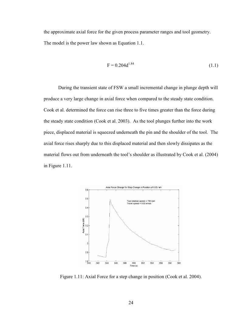
the approximate axial force for the given process parameter ranges and tool geometry.

The model is the power law shown as Equation 1.1.

F = 0.204d1.84 (1.1)

During the transient state of FSW a small incremental change in plunge depth will

produce a very large change in axial force when compared to the steady state condition.

Cook et al. determined the force can rise three to five times greater than the force during

the steady state condition (Cook et al. 2003). As the tool plunges further into the work

piece, displaced material is squeezed underneath the pin and the shoulder of the tool. The

axial force rises sharply due to this displaced material and then slowly dissipates as the

material flows out from underneath the tool’s shoulder as illustrated by Cook et al. (2004)

in Figure 1.11.

Figure 1.11: Axial Force for a step change in position (Cook et al. 2004).

25

The axial force is also linked to the rotation rate and traverse rate of the tool.

Although these process parameters have less of an influence on the axial force than the

plunge depth, they can alter the steady state axial force when changed by large amounts.

Figure 1.12 and Figure 1.13 illustrate the changes in axial force as a function of tool

rotation and linear velocity as determined by Cook et al. (2004). Intuitively it can be

concluded as the tool rotates faster; the addition heating generates higher temperatures

and softer conditions in the metal, thus lowering the required axial force. However, there

is a drawback to increased rotation rate. At high rotational rates, undesirable weld flash

can be created when the metal is detached and expelled from underneath the shoulder of

the rotating tool. At high rotational speeds the shoulder surface shears off a thin layer of

the work piece. Once this sheared layer of metal is expelled from underneath the tool’s

shoulder and off of the work piece’s surface, it is referred to as weld flash.

The linear velocity of the tool as it traverses along the weld seam also contributes

to the value of the axial force. As reported by Crawford et al. (Crawford et al. 2006)

there is a direct relationship between the tool velocity and the axial force. A slower

traversing tool will input more heat energy into the work piece than a faster moving tool.

With the increase in temperature, the axial force will be lower assuming the plunge depth

remains constant. At higher velocities, less heat is input into the work piece and the weld

zone is much colder. This colder welding condition generates more force both in the

axial and traverse directions. The increase in the traverse force is due to the increased

resistance of the material to flow through the die cavity to the back side of the tool’s pin.

26

Figure 1.12: Axial force as a function of tool rotation speed. (Cook et al. 2004)

Figure 1.13: Axial force as a function of tool’s traverse speed. (Cook et al. 2004)

27

In addition to the process parameters, the tool’s geometry and work piece’s

material properties also have influence in determining the value of the axial force. For a

given traverse and rotation rate, a larger tool pin profile with more surface area will

require higher axial loads. Likewise a more dense work piece material will need higher

forces to plastically deform and then forge together the parent pieces than a less dense

material.

Axial Force Control verses Position Control

Force control is needed in a FSW process when the axial force is very sensitive to

the application method. Robotic applications are a prime example of this sensitivity.

Typically robots are of a compliant nature and do not exhibit great stiffness. Due to their

inherent compliant and limited load capacities, use of robots in FSW applications has

been restricted. As a robot operating under position control articulates a FSW tool in a

weld seam, deflection will occur within the robot’s arms and joints. Compensation for

the deflection is not executed in the controller, because the position feedback comes from

encoders located in the robot’s axis motors. The deflection in the arms and joints is not

sensed and thus no position compensation is performed. This deflection will lead to

variation in the weld tool position as well as the applied axial force. Axial force and tool

shoulder contact with the work piece is needed in order to forge the plastically deformed

parent metals together.

When there is not an adequate amount of forging force in the die cavity,

volumetric material voids such as worm holes can occur. These voids create porous

conditions which negatively impact the structurally integrity of the weld. With

28

insufficient force, the frictional force between the tool shoulder and the work piece is

reduced. This leads to less heat generation and lower temperatures inside the die cavity.

The lack of heat does not aid the deformation of the work piece because the material

remains in a hardened state. In addition, the colder welding condition does not promote

the mixing and forging together of the plasticized metal. The likelihood of volumetric

defects due to insufficient axial force can be reduced with the use of force control.

Force control can successfully be utilized in high volume manufacturing

applications where there is a lot of variation in the material being welded. The variation

can be in the form of part thickness, surface profile, temperature, or in positioning of the

part as it is located in the weld fixture. Force control is a robust process that can

compensate for work piece variation, joining imperfections along the faying surface as

well as the inherent compliance in the robot.

With force control, a measured force at the tool is used as a feedback signal for

the controller. Any change in the desired force at the tool, is sensed and a processed error

signal from the force controller adjusts the robot position to maintain the desired force at

the tool. When compared to position control, force control provides more flexibility due

to its ability to adapt to varying material and process conditions. If process adaptation

with position control is utilized, material imperfections, variance in part location and

large surface changes would have to be detected with some type of vision sensor and then

the control algorithm would have to vary the position of the tool’s depth. A force control

system eliminates the need for the vision sensors and the complex control algorithm.

If the tool’s plunge depth into the work piece remains constant, sufficient force is

automatically maintained when traditional machine tools under position control are used

29

in the FSW process. Their rigidity is inherent due to the designed intent to manufacture

precision machine parts. A machine tool such as a computer numerically controlled

(CNC) milling machine when applied to FSW controls the depth of the tool into the

metal. The force becomes a function of the tool’s depth. Position control is popular and

widely used in many FSW applications. Typically, it is used when there is not much

variation in the parts being welded or when there is a wide range of acceptable weld

conditions. As an example, if the tool’s plunge depth changed due to an increase in part

thickness; more weld flash will be generated. If the additional weld flash and increase in

weld force is acceptable, position control is a good control process to use. However, if

the weld flash and increase in force is unacceptable, force control would be the preferred

control process. With position control, plunge depths are set quite generously to account

for the tolerance in material thickness. Another advantage of position control over force

control is its stability. The weld controller has a greater likelihood of becoming unstable

under force control (Smith 2007). This instability can lead to defects by either the tool

penetrating too far into the work piece or withdrawing from the work piece. In either

case the resulting weld quality is greatly diminished.

For advanced FSW machines, both force and position are viable control

architectures. As previously mentioned the tool’s depth into the material and the axial

force are tightly coupled together. Due to the possibility of volumetric defects, axial

force is a more important weld parameter than weld depth, although the two are closely

related. An intelligent processing strategy would call for primary control of the axial

force and secondary control of the tool’s depth. Small variations in depth are tolerable in

most FSW applications while large variations in force are not. Since axial force is related

30

to tool depth, corrections to the force would be made by adjusting the tool’s position.

The variations in depth would be very small because of the extremely stiff environment

of the work piece. Thus a small adjustment to the tool’s depth would result in a large

adjustment in the axial force. With position being secondary in the controls hierarchy,

upper and lower position constraints would be established to maintain the tool’s position

within an acceptable tolerance.

Force Control Theory

As previously noted it is very important to use force control to adapt to material

surface variance and compliance in either the machine tool or the robot. Force control

provides flexibility in the FSW process where as position control is limited to ideal

conditions or when there is a wide range of acceptable welding conditions. A standard

architecture for force control that could be used on a robot or CNC milling machine

might take the appearance shown in Figure 1.14 (Cook et al. 2004). The servo force

control resides outside the position control loop. This architecture allows the adaptation

of force control through retrofitting existing position controlled machine tools or robots.

The force error signal from the force controller is sent to the position controller as the

reference position. It is attractive because of its simplicity and ease of integration with

the position control system.

A more sophisticated approach to force control is shown in Figure 1.15 (Craig

2005). This approach is based upon a mass-spring system but it can be applied to the axis

of a milling machine or a FSW machines similar to ones shown in Figure 1.16.

31

Figure 1.14: Force controller architecture (Cook et al. 2004).

Figure 1.15: Sophisticated force control architecture (Craig 2005).

When applied to this type of equipment, m represents the mass of the z-axis quill

and spindle, z is the spinning tool axis, ke is the spring constant of the work piece and the

disturbance force fdist is the coulomb friction fr inside the quill. The system dynamics can

be described by Equation 1.2.

32

Figure 1.16: A Transformation Technologies Inc. RM-1 FSW machine (Transformation Technologies, Inc 2009) and a Bridgeport EZ Vision CNC mill (Hardinge 2009).

f = mz˝ + kez + fr (1.2)

Generally machine tools of this nature have their quills counterbalanced, thus for

this analysis the effect of gravity is ignored. To begin the derivation of force control, the

dynamics will be simplified by assuming the work piece’s spring force is constant. This

simplification will allow for analysis and insight into the behavior of force control for

FSW. The objective of the control system is to control the force fe acting on the work

piece. The force fe is defined in Equation 1.3 as the resulting force when the tool plunges

a depth z into a work piece with a spring rate ke.

fe = kez (1.3)

33

After substituting Equation 1.3 into Equation 1.4 the system’s dynamics is

defined in terms of the force desired for control. The force fe shown in Equation 1.4 is

the process variable that must be controlled to obtain good welds.

f = mke-1fe˝ + fe + fr (1.4)

To control the axial force fe, a partitioned control scheme will be used (Craig

2005). The controller is divided into a model and a servo portion. The control law is

defined by Equation 1.5.

f = αf΄ + β (1.5)

The model portion is subdivided into an alpha (α) and beta (β) portion. The α and

β variables are defined by Equation 1.6 and Equation 1.7 while f΄ is the input into the

system.

α = mke-1 (1.6)

β = fe + fr (1.7)

The servo portion of the control law is defined by Equation 1.8 and Equation 1.9

where fd is the desired force.

ef = fd - fe (1.8)

34

f΄ = fed˝ + kvef΄ + kpef (1.9)

The expanded control law can be expressed by substituting the servo portion

given by Equation 1.9 into the control law given by Equation 1.5. The results are

expressed in Equation 1.10 where Kv is the derivative gain, Kp is the proportional gain, ef

is the force error and e΄f is the derivative of the force error.

f = mke-1[fd˝ + Kve΄f + Kpef] + fe + fr (1.10)

Upon observation of Equations 1.4 through 1.7, it can be seen that f΄ must also

equal fe˝. With this observation Equation 1.4 and Equation 1.10 can be equated. The

closed loop system of the controller plus the physical system can be expressed in the

linear form of Equation 1.11.

ef˝ + Kve΄f + Kpef = 0 (1.11)

However, it would be difficult to apply this control approach because of two

reasons. First, the value of the fiction force would be extremely difficult to determine.

Secondly, a constant force value is desired. Thus the terms fd˝ and fd΄ are set to a value of

zero.

With a work piece that has a high stiffness the proposed control can be modified

slightly. In the model portion of the controller, β can be set equal to the desired force fd.

The modified and newly proposed control law is given in Equation 1.12.

35

f = mke-1[fd˝ + Kve΄f + Kpef] + fd (1.12)

To analyze the effect of this change in a steady state condition, Equation 1.4 and

Equation 1.12 are equated. With steady state analysis the time derivatives of ef are zero.

The result of the equated equations is reduced to the form given in Equation 1.13.

ef = fr / (1 + mke-1Kp) (1.13)

Equation 1.13 represents the steady state error. With the application of FSW

using a conventional milling machines and small FSW machines, the ratio mke-1 of the

quill mass to the work piece stiffness will be quite small. In addition, when compared to

the quill mass and the work piece stiffness, the friction of the quill mass will also be

small. Equation 1.13 shows the results of these two conditions will lead to a relatively

small steady state error. If it is desired to further improve the systems performance and

eliminate the steady state error, an integral term could be applied to Equation 1.12.

One last modification can be made to the control law to make it more applicable

to FSW. Due to the physical nature of FSW, sensors measuring the axial force might

produce a rather noisy signal. The computed derivative of the signal would be greatly

altered by the noise. A better method would be to simply use the derivative of the tool

position. This is plausible because the resulting axial force is related to the tool depth.

The rate of depth change will be proportional to the rate of force change assuming linear

36

conditions. The revised control law is expressed in Equation 1.14 and shown in a block

diagram form with Figure 1.7.

f = m[Kpke-1ef - Kvz΄] + fd (1.14)

Figure 1.17: Applied force control architecture (Craig 2005).

The problem with applying this approach to FSW is the nonlinear relationship

between plunge depth and axial force. Most applications of force control used today are

only applied during the steady state conditions of the welding process. Constant process

parameters of tool rotation rate, traverse rate and plunge depth are used to create steady

state conditions. During steady state conditions under force control the axial force is held

constant by making adjustments in the tool’s plunge depth. Typically the servo portion

of the force controller is activated once the desired steady state force is achieved. The

servo control then acts as a regulator to maintain this value. However, with this

architecture it is possible to input a time varying force as the desired force. Successful

applications of force control to steady state FSW have been documented (Zhao et al.

2007), but applications to FSW are not well suited with this type of architecture. This

architecture requires the spring rate of the material to be a known constant. Thus the

37

wide spread implementation of this architecture to FSW is not practical. It should only

be limited to a specific manufacturing process where prior testing has been conducted to

establish the operating parameters and unknown variables.

Research Presented

The research presented in this dissertation provides an in depth examination of

force control as applied to FSW. Three separate modes of force control are designed and

implemented on a retrofitted Milwaukee Model K milling machine. Each force control

mode uses a different controlling variable. Along with the three modes of force control,

an alternative control method (torque control) is presented.

The dissertation is organized into seven chapters. Chapter I is an introduction and

literary review of FSW. Chapters II through VI are a collection of papers examining the

various modes of force control. Chapter VII is a conclusion based upon the result

presented in Chapter II through VI.

Chapter II presents a previously unexplored method of force control. The research

investigates the use of tool traverse speed as the controlling variable instead of plunge

depth. To perform this investigation, a closed loop proportional, integral plus derivative

(PID) control architecture was established and tuned using the Ziegler-Nichols method.

Welding experiments were conducted by butt welding ¼ inch x 1 ½ inch x 8 inch

samples of aluminum 6061 with a ¼ inch threaded tool and a ¼ inch Trivex tool.

Results show the control of axial force via traverse speed is feasible and

predictable. The resulting system is more robust and stable when compared to a force

controller that uses plunge depth as the controlling variable. A standard deviation of 41.5

38

Newtons was obtained. This variation is much less when compared to a standard

deviation of 129.4 Newtons obtained when using plunge depth. Using various

combinations of PID control, the system’s response to step inputs was analyzed. From

this analysis, a feed forward transfer function was modeled that describes the machinery

and welding environment.

From this research a hypothesis is presented regarding heat control as a by

product of force control via traverse speed. A relative measurement of heat is obtained

with the feedback of axial force. It is hypothesized that while under force control the tool

deposits heat per unit length of weld seam according to the control signal. The result is

uniform heating along the weld seam.

It is concluded that the key enablers for force control via traverse speed are the

unidirectional behavior and load dynamics of the traverse motor. Larger bandwidths and

more stable weld conditions emerge when using traverse speed instead of plunge depth to

control the force. Force control of FSW via traverse speed has importance in creating

efficient manufacturing operations. The intelligence of the controller naturally selects the

most efficient traverse speed.

Chapter III examines the control of axial force via plunge depth adjustment. The

research presented in this paper identifies the key enablers for successful and stable force

control of FSW. To perform this research, a closed loop PID control architecture was

established and tuned using the Ziegler-Nichols method. Welding experiments were

conducted by butt welding ¼ inch x 1 ½ inch x 8 inch samples of aluminum 6061 with a

¼ inch threaded tool.

39

The experimental force control system was able to regulate to a desired force with

a standard deviation of 129.4 Newtons. From the experiments, it is determined that tool

geometry and position are important parameters influencing the performance of the force

controller. From the results four key enablers are identified for stable force control of

FSW. The key enablers identified are:

• Maintaining a portion of the tool’s shoulder above the work piece surface.

• A smooth motion profile for plunge depth adjustment.

• Increasing the lead angle for flat shoulder tools.

• Establishing positional constraints.

It is concluded that successful implementation of the force control in future FSW

systems, can be obtained by establishing and adhering to these key enablers. In addition

to robotic benefits, force control via plunge depth adjustment reduces weld flash and

improves the appearance of the weld.

Chapter IV examines force control of FSW via varying the tool’s rotation speed.

The closed loop PID control architecture was tuned using the Ziegler-Nichols method.

Welding experiments were conducted by butt welding ¼ inch x 1 ½ inch x 8 inch

samples of aluminum 6061 with a ¼ inch Trivex tool.

The results indicate it is possible to control the axial force by adjusting the tool

rotation speed. With the presented experimental force controller, the axial force was able

to be maintained within a standard deviation of 132 Newtons. However to achieve this

40

control, a rather large plunge depth was needed. The large plunge depth resulted in

excess flash.

It is concluded that force is controlled by varying the rate of heat generation. In

addition, the FSW machine needs to be capability of producing a large range of tool

rotation speeds in order to adequately control the axial force over a wide range of varying

thermal conditions within the work piece.

Chapter V compares the force response from the controlling variables of traverse

speed, rotation speed and plunge depth. Welding experiments were conducted by butt

welding ¼ inch x 1 ½ inch x 8 inch samples of aluminum 6061-T6511 with a ¼ inch

FSW tool. Along with the force analysis, energy models and material testing are

presented.

The results indicate that force control via traverse speed is the most accurate and

as a byproduct heat distribution control along the weld seam occurs. Force control via

plunge depth is the least accurate but it compensates for machine and robot deflection.

Tensile test data shows that greater strength can be obtained through force control via

rotation speed.

It is concluded that force is maintained by keeping the amount of tool surface area

in contract with the work piece constant throughout the welding process when plunge

depth is used as the controlling variable. Force is maintained by varying the rate of heat

generation when rotation speed is used as the controlling variable. Lastly force is

maintained by changing the amount of heat deposited per unit length along the weld seam

when traverse speed is used as the controlling variable. Successful robotic FSW requires

41

selecting the appropriate controlling variable and reducing the sensitivity of the

interaction between the tool and the work piece.

Chapter VI presents and an alternative to axial force control. Torque control is

examined and presented as viable option for robotic FSW. The results indicate that

controlling toque produces an acceptable weld process that adapts to the changing surface

conditions of the work piece. For this experiment the torque was able to be controlled

with a standard deviation of 0.231 Newton – meters. In addition the torque controller

was able to adjust the tool’s plunge depth in reaction to a 1 millimeter step disturbance in

work piece thickness.

It is concluded that the feedback signal of torque provides a better indicator of

tool depth into the work piece than axial force. Torque is more sensitive to tool depth

than axial force. Thus it is concluded that torque control is better suited for keeping a

FSW tool properly engaged with the work piece.

Survey of Literature

Since FSW is a relatively new technology there is a large amount of active

research being conducted. Numerous publications can be found regarding the

development of models and equations describing the joining process. However there is

no consensus on a single FSW model among the scientific and engineering community.

In regards to robotic and force control applications of FSW, few published works are

available. A survey of published papers is summarized below.

Investigation into characterizing the FSW environment for the purpose of robotic

application was previously conducted at Vanderbilt University. The work was published

42

in three papers. These papers identify and provide incite into the fundamental problems

that must addressed for the successful application of robotic FSW. A key theme in each

of the papers is the need for force control. A summary of the papers with their

conclusions is outlined below.

The first paper “Controlling Robotic Friction Stir Stir Welding (Cook et al. 2003)

presents a series of experiments that examine the relationship between process

parameters and axial force. Their results establish that axial force increases with faster

traverse speeds and slower rotation speeds. Another experiment allows the

characterization of axial force with changes in plunge depth. They note how a small

change in plunge depth produces a very large change in axial force. An interesting aspect

to this relationship is how the force subsides to near its value prior to the change in

plunge depth. They note how this transient condition could cause stability issues for a

force controller. Because of the large force change with plunge depth, they conclude that

using force feedback is necessary for robotic FSW.

The second paper “Robotic Friction Stir Welding” (Cook et al. 2004) discusses

methods of force feedback. One method proposes adding a force control loop outside of

the existing position control loop of a robot. The other method utilizes the Jacobian

relationship of the manipulator. The Jacobian matrix relates the actuator torques to the

forces applied at the face plate of the robot.

The third paper “Modeling of Friction Stir Welding for Robotic Application”

(Crawford et al. 2006) presents two models; a Couettee flow and a Visco-Plastic flow

model. Both of these were created using the fluid dynamics software package FLUENT.

43

The results of the models correlated with behavior observed in physical experiments.

However the results more closely matched the Visco-Plastic model.

Successful implementation of force control to FSW has previously occurred in a

laboratory. Zhao et al. developed a controller from experimental data obtained while

welding using an ABB IRB 940 Tricept robot (Zhao et al. 2007) (Zhao et al. 2008).

There work is detailed in the papers titled “Design and Implementation of a Nonlinear

Axial Force Controller for Friction Stir Welding Processes” and “Design and

Implementation of Nonlinear Axial Force Controllers for Friction Stir Welding

Processes”. With their experimental data they were able to create static and dynamic

models of the welding system. With these models, they used a Polynomial Pole

Placement method to design the controller. The controller was then implemented in a

Smith Predictor – Corrector structure to compensate for the system delays. Their

controller was able to maintain a constant axial force as the tool crossed gaps in the work

piece.

Another successful implementation of force control to robotic FSW was

documented in the paper titled “A Robot Prototype for Friction Stir Welding (Soron and

Kalaykov 2006). Soron and Kalaykov use an ABB IRB-7600-500 serial robot for their

experimentation. They replace the sixth axis with FSW tooling including an ATI Omega-

190 force and torque sensor. Two types of robot controllers are used. The first was the

ABB S4C + which has force control based on an existing path corrector option in the

program. The force control algorithm was a standard proportional plus integral control.

The second controller was the ABB IRC5 which uses force control for standard industrial

operations such as grinding and assembly. The pre-existing software package for these

44

operations has the force control embedded. They adapted grinding and assembly

instructions to FSW to utilize the commercially developed software for force control of

FSW. They conclude it is feasible to implement force control. In addition using the

standard industrial robot creates benefits such as a flexible workspace, fast programming

and cost effectiveness for a 3-dimensional solution to FSW. However they noted a few

drawbacks such as force oscillations, predicting penetration depth and defining the

welding trajectory in 3-dimensions with high precession.

Figure 1.18: Robotic FSW setup by Smith (2000).

Other documented cases of force control include work by Smith (2000), Smith et

al. (2003), Talwar et al. (2000) and by Strombeck et al. (2000). Smith reported in the

paper “Robotic Friction Stir Welding using a Standard Industrial Robot” the ability to use

actuator torques as a measurement of the FSW force through the Jacobian relationship

(Craig 2005). The process was limited by the computation time needed. The controller

was able to produce an updated control signal up to 2 Hz. Smith used an ABB IRB 6400

robot with its open architecture to implement force control. With this configuration he

45

was able to weld 3 mm thick aluminum. He concluded that the update time is not

adequate for force control during the plunging operation and that deflections in the

traverse direction must be overcome with programming offsets.

The experimental setup is shown in Figure 1.18 and the force control results are

shown in Figure 1.19. In Figure 1.19 the force control is activated after the plunge

operation is complete and the tool begins to traverse forward.

Figure 1.19: Force control results by Smith (2000).

Smith et al. (2003) used an ABB IRB 7600 articulated arm robot to successful

integrate a FSW system and implement force control. An important enabler of the

system was a software package (StirWareTM) specifically designed for FSW. They were

able to weld under a programmed 3 – 4 mm change in work piece height over the length

of the weld. The results are shown in Figure 1.20. Strombeck et al. (2000) used a

parallel robot to perform force controlled FSW. However the parallel designed robot’s

46

work space was more constricted as compared to an articulating arm robot. Talwar et al.

(2000) used an electro-mechanical force actuator on a 5-axis CNC mill to control the

axial force while producing lap welds.

A different force control approach was taken by Ding et al. (2002). They

developed and patented a force control device that controls force via varying the length of

the pin. The force is measured by a sensor at the end of the pin. The variable length pin

allows for a variety of work piece thicknesses to be welded.

Figure 1.20: Force control results by Smith et al. (2003).

Force control related publications have been authored by Takahara et al. (2008),

Kruger et al. (2004) and Arbegast (2005). Takahara et al. examined the properties of

welds when different control approaches were taken to 3-dimensional welding. They

47

examined right angle directional changes on a curved surface. They concluded that the

tool motion should be continuous when it approaches changes in direction and that

deviations from idea parameters such as lead angle produce acceptable results.

Kruger et al. (2004) presented modular software architecture for the control of

FSW. The emphasize the requirement for an online process monitoring system that can

provide feedback to a controller such that a FSW machine can adapt to changing

conditions in the welding process. They point out that CNC machine tools do not have

this capability. Their modular design divides the controller into 6 layers. The layers are:

communication interface, device interface, machine interface, process interface, data

interface and user interface.

Arbegast (2005) presents statistical data that correlates variations in process

forces to process flaws. His findings create the possibility for online process monitoring

algorithms that can detect flaws and then adjust the welding parameters. One of his most

intriguing findings is the Fourier analysis of the y-force fluctuations. He found a

correlation between low frequency force events and wormhole defects. The magnitude

and quantity of the events was found to be related to the size of the wormhole.

Force control is needed to maintain sufficient axial force. Without the proper

force material voids and worm holes can form. In the paper titled “Three-Dimensional

Modeling of Void Growth in Friction Stir Welding of Stainless Steel” the authors He et

al. (2007) conclude the effect of the tool shoulder on void growth is significant. Their

models predict high porosity throughout the weld when no shoulder is contacting the

work piece. Their conclusions support the importance of force control. They determine

through their models that voids tend to form on the advancing side of the pin. In addition

48

if the tool’s pin has threads present, these voids move to the bottom surface of the weld

nugget.

The paper “Influences of Tool Pin Profile and Welding Speed on the Formation of

Friction Stir Processing Zone in AA2219 aluminium alloy” (Elangovan and

Balasubramanian 2008) concludes the geometric configuration of the tool’s pin has a

significant influence on the quality of the weld. Their results show a square profiled pin

produced defect free welds within the processing parameters of the experiment. When

compared to a straight cylindrical pin, a tapered cylindrical pin, a threaded cylindrical

pin, a triangular pin, the square pin produced welds with a finer grain structure, larger

tensile strength and higher hardness. The finer grain structure and better mechanical

properties are attributed to the pulsating stir action of the square pin.

Another article relating tool geometry to process forces and weld quality is

“Characterization of the Influences of FSW Tool Geometry on Welding Forces and Weld

Tensile Strength Using an Instrumented Tool” (Hattingh et al. 2008). In this study

several tools with different pin geometries were used to produce welds in 6 mm thick

5083-H321 aluminum alloy. Experimental results show the pin geometry to have an

affect on both the direction and magnitude of the force on the tool. In addition,

depending on the tool geometry, welds with 97% of the parent metals strength were

obtained.

Research by Pew et al. (2007) and Pew (2006) empirically models torque for three

different aluminum alloys. The FSW model details the relationship between process

parameters and torque. The torque input is then used to create a weld power and heat

input model. Their results show the traverse rate and rotation rate of the tools has little

49

effect on the heat input at high traverse rate. However at low traverse rates, decreasing

the rotation rate or increasing the traverse rate significantly decreases the heat input. The

heat input trends are supported with measurements of the heat affected zone of the weld.

In regards to controlling torque, a United States Patent Application was filed by

Buford et al. (2004) of the Boeing Company. Their patent controls actuator torque for

the FSW device in order to maintain a constant welding condition. For instant if the

FSW device is a CNC machine tool, their patent maintains a constant actuator torque for

the plunge depth axis system. They are able to correlate through experimental testing the

relationship between axial force and actuator torque for a particular welding operation.

50

CHAPTER II

ENABLING OF ROBOTIC FRICTION STIR WELDING: THE CONTROL OF WELD SEAM HEAT DISTRIBUTION BY TRAVERSE SPEED

FORCE CONTROL

William R. Longhurst, Alvin M. Strauss, George E. Cook

American Society of Mechanical Engineers Journal of Dynamic Systems Measurement

and Control. Current Status: Submitted May 28, 2009. Under Review.

Abstract

Friction Stir Welding (FSW) joins materials by plunging a rotating tool into the

work piece. The tool consists of a shoulder and a pin that plastically deforms the parent

materials and then forges them together under the applied pressure. To create the

pressure needed for forging, a rather large axial force must be maintained on the tool.

Maintaining this axial force is challenging for robots due to their limited load capacity

and compliant nature. To address this problem, force control has been used and

historically the force has been controlled by adjusting the plunge depth of the tool into

the work piece.

This paper develops the use of tool traverse speed as the controlling variable

instead of plunge depth. To perform this investigation, a FSW force controller was

designed and implemented on a retrofitted Milwaukee Model K milling machine. The

51

closed loop proportional, integral plus derivative (PID) control architecture was tuned

using the Ziegler-Nichols method.

Results show the control of axial force via traverse speed is feasible and

predictable. The resulting system is more robust and stable when compared to a force

controller that uses plunge depth as the controlling variable. A standard deviation of 41.5

Newtons was obtained. This variation is much less when compared to a standard

deviation of 129.4 Newtons obtained when using plunge depth. Using various

combinations of PID control, the system’s response to step inputs was analyzed. From

this analysis, a feed forward transfer function was modeled that describes the machinery

and welding environment.

From these results a technique is presented regarding heat control as a by product

of force control via traverse speed. A relative measurement of heat is obtained with the

feedback of axial force. It is hypothesized that while under force control the tool deposits

heat per unit length of weld seam according to the control signal. The result is uniform

heating along the weld seam.

It is concluded that the key enablers for force control are the unidirectional

behavior and load dynamics of the traverse motor. Larger bandwidths and more stable

weld conditions emerge when using traverse speed instead of plunge depth to control the

force. Force control of FSW via traverse speed has importance in creating efficient

automatic manufacturing operations. The intelligence of the controller naturally selects

the most efficient traverse speed.

52

Introduction

Friction Stir Welding (FSW) is a solid state joining process that utilizes a rotating

non-consumable tool to plastically deform and forge together parent metals. FSW tools

contain two necessary features for the joining process. These features are a shoulder and

a pin (or probe). The shoulder is used to generate heat and forging pressure within the

localized welding area. The pin which resides beneath the shoulder is used to plastically

deform the parent metals of the work piece. Plastic deformation takes place as the pin

shears off thin layers of material from the parent metals and rotates them to the backside.

At the backside of the pin, the pressure from the shoulder consolidates the deformed

parent metals.

For the case of butt welding together two plates, the FSW tool is plunged into the

work piece at the intersection of the two plates. When fully plunged into the work piece,

the pin is completely submerged below the surface, while the shoulder resides at the

surface or just below it. During the joining process the tool traverses along the faying

surface with the pin’s axis of rotation in the same plane as the faying surface. Once the

tool has reached the end of the weld seam, it is extracted. After extraction, a solid joint

exists between the two plates.

Since its inception in the early 1990’s, FSW has emerged as a viable welding

process for many metals. Historically the process utilizes the control of three process

parameters. These parameters are the tool’s plunge depth, traverse and rotation speed.

As FSW technology continued to develop, axial force became an important process

variable that needed to be controlled in closed-loop architecture. Force control is

particularly important for robotic application of FSW because of its compliant nature

53

(Cook et al. 2004). Robotic compliance makes the application of FSW very challenging

if not impossible without force control. Without a sufficient axial force acting through

the tool, the forging of the plastically deformed work piece would not occur. As a robot

continually repositions the FSW tool along the weld path, deflection in the robot’s

linkages and joints would cause undetectable plunge depth variations. FSW tool plunge

depth variations lead to axial force variations and typically insufficient forging pressure

beneath the tool’s shoulder. Hence with insufficient forging pressure, severe welding

defects and inadequate joining may occur. With non-robotic applications, an adequate

axial force is typically achieved with the combination of a sufficient plunge depth of the

tool into the work piece and the structural rigidity of the applying machine.

Figure 2.1: Axial force as a function of the tool’s traverse speed.

Past research at Vanderbilt University by Cook et al. (2003), has shown the axial

force to be a function of tool plunge depth, traverse speed and rotational speed. Fig. 2.1

54

illustrates the relation between axial force and the traverse speed. As the traverse speed

is increased, the axial force increases as well.

The experimental results show the welding environment to be stiffer for lower

tool rotation speeds. This is due to less heat generation and the subsequent reduction in

the softening of the work piece material. For a given rotational speed the axial force

changes as a function of traverse speed. The results suggest that large changes in axial

force can be obtained by varying the traverse speed. These changes in axial force are

greater at slower rotation speeds and less at higher rotation speeds.

Historically, force control of FSW has been accomplished by varying the plunge

depth of the tool. Examples are found in the published work by Smith (2000), Soron and

Kalaykov (2006) and Zhao et al. (2007). Each of these developed and implemented a

force control architecture using plunge depth as the controlling variable. All were able to

conclude it was feasible to implement FSW force control. However, using plunge depth

as the controlling variable presents several challenges. Soron and Kalaykov concluded

that even with the implemented action of force control to a robotic FSW system, axial

force oscillations will exist when the tool makes contact with the material. They also

noted that the penetration depth is hard to predict due to the positioning error of the robot.

Zhao et al. presented a non-linear axial force controller they developed and implemented

for a FSW process. They were able to experimentally characterize the static and dynamic

behavior of the interaction between the FSW tool and the work piece. With this

information and using an open architecture control system they were able to design a

controller using polynomial pole placement. Good results were obtained, but to handle

the non-linear transient response when the tool’s plunge depth changed, the control

55

system had to incorporate experimentally obtained dynamic parameters. Thus the open

architecture of the control platform was needed in order to implement this force

controller and the controller parameters were specific to their experimental setup.

To the authors’ knowledge, there has not been any published research on the force

control of FSW using the tool’s traverse speed as the controlling variable. The goal of

this research is to create a FSW force control architecture that utilizes the tool’s traverse

speed as the controlling variable. Since the controlling variable is the tool’s traverse

speed, the plunge depth remains constant.

Presented in this research is the experimental force control architecture. From

this experimental architecture the controlled response of the system is characterized and

the contributing elements to the response are identified. Comparisons are drawn between

the performance of this experimental FSW force control system that utilizes traverse rate,

and a FSW force control system that utilizes the plunge depth as the controlling variable.

It is concluded that this control strategy provides a very robust and stable architecture for

force control. Lastly a hypothesis is presented along with supporting evidence that heat

distribution control is obtained as a byproduct of force control when the traverse speed is

used as the controlling variable.

Experimental Configuration

The experiments were conducted on the FSW system at Vanderbilt University.

The FSW system is a Milwaukee Model K milling machine that has been retrofitted with

more advanced motors and instrumentation. The system is shown in Fig. 2.2. These

retrofits were previously added to automate the system and provide a programmable

56

platform for FSW experimentation. At the top of the control hierarchy is a master

computer that enables all of the systems subcomponents such as the motor drive

controllers and instrumentation. The master computer is a Dell Precision 340 that uses

Microsoft Windows XP as its operating system. The welding and force control code was

written in C#. A graphical user interface within the C# software allows the operator to

select the desired welding parameters for the pending operation. These parameters

include the FSW tool’s rotation speed, traverse speed, plunge depth and weld path

position.

Figure 2.2: FSW machine at Vanderbilt University.

57

The traverse axis coincides with the milling machine worktable’s cross axis. The

worktable resides in its saddle by sliding dovetail joints and is driven by a power screw.

The power screw is rotated via a system that consists of a belt and pulley attached to the

shaft of the power screw. A 1 horsepower (745.70 Watts), 6.02 reduction Syncrogear

gear motor is attached to the drive pulley. The gear motor is controlled by a Cutler-

Hammer MVX9000 Sensorless Vector variable frequency drive (VFD). Command

signals are sent directly from the master computer to the VFD. Traverse position is

obtained from a string potentiometer. Analog position data from the potentiometer is

feed into a sensor box were it is converted to a digital signal prior to being sent to the

master computer.

Welding force data is collected through a Kistler Rotating Cutting Force

Dynamometer. The dynamometer collects x-axis force, y-axis force, z-axis force as well

as the torque about the z-axis. The analog signal from the dynamometer is sent to a signal

conditioning box where it is converted from an analog signal to a digital signal. Once

converted, the data is sent to a separate computer where the data is sorted, recorded, and

displayed before being sent to the master computer.

An overview of the closed loop force control system is illustrated by the control

block diagram of Fig. 2.3. Within the master computer a desired z force is selected. The

desired force value is subtracted from the actual z force value to obtain a force error. The

force error signal is then processed in the control law. The resulting processed control

signal is then multiplied by a factor of 0.05 to translate the signal from Newtons of force

to desired inches per minute of traverse speed. The desired inches per minute is

converted to the corresponding frequency and then sent to the VFD. The VFD produces

58

the desired change in traverse speed to obtain the desired value of z force in the welding

environment. The dynamometer reads the resulting force and returns it to the master

computer where it is once again compared to the reference signal.

Figure 2.3: Block diagram of force control via traverse speed.

The measured z force signal was very noisy. This noise makes the process of

applying derivative control to the system very difficult. The noise would simply be

amplified by the controller. To address this problem, a filter was implemented. The filter

is a five point moving average of the z force with an interrupt frequency of 3.33 Hz. For

this experimental setup these filter parameters were found to provide adequate noise

reduction without adding too much phase lag in the signal.

The control law consisted of proportional, integral plus derivative (PID) control.

Due to the retrofitted nature of the FSW system there are several unknown parameters

that could not be accurately modeled to create a non-linear modeled based control

system. For instance, the force control loop resides outside the control loop for the

traverse drive. The Cutler-Hammer VFD uses its own proprietary control techniques to

59

drive the motor. Thus, obtaining the parameters of the VFD as well the physical

parameters of the traverse motor, gear box, belt drive, and power screw would require an

extensive amount of testing and analysis. In addition, the time needed for signal

processing and transmission through the master computer, dynamometer, sensor box and

the VFD would also have to be experimentally determined. With all of these variables to

consider the potential performance of a model based controller might not be much better

than a standard PID controller. For this experimentation to create and investigate the

performance of z axis force control via traverse speed, PID control architecture was

chosen as the best option.

To address the transport delay between the initiation of the control signal and the

change in force, a simple delay of 1 second in the control update time was utilized. The 1

second delay allowed the FSW tool to change speed and a change in z force to occur.

The delay in the control signal update proved to be effective without the need of adding a

more complicated controls approach such as a Smith Predictor-Corrector (Ogata 2002).

To tune the PID force controller and achieve optimum control, the Ziegler-

Nichols tuning process was used (Ogata 2002). The Ziegler-Nichols tuning process

called for the controller to use only proportional gain while welding. While using

proportion control only, a critical gain value was experimentally determined through trial

and error. Over the course of several welds, the gain was steadily increased until the

resulting z force achieved sustained oscillation. The sustained oscillation constituted

marginally stable behavior. The resulting control gain and time period between

oscillations was recorded and used to calculate PID gains for the controller. The

resulting PID control law is shown in Eq. (2.1). In Eq. (2.1), Kp is the proportional gain,

60

Ki is the integral gain, Kd is the derivative gain, e is the error and u is the resulting control

signal as a function of time t.

Kp e + Ki ∫e + Kd e΄ = u(t) (2.1)

For this force control research, experiments using two different FSW tools were

performed. The two tools with their contrasting size and geometry provided insight into

the dynamics of the FSW system. The first tool consisted of a slightly undersized 1/4

inch (6.35 mm) Trivex pin with a flat 5/8 inch (15.875 mm) diameter shoulder. The

Trivex profile geometry is similar to an equilateral triangle but with its edge surfaces

slightly convex. The pin with its Trivex geometry was 0.235 inches (5.969 mm) long by

0.210 inches (5.334 mm) across its widest point. The second tool was larger in size as

compared to the 1/4 inch (6.35 mm) Trivex. The second tool consisted of a 1/4 inch

(6.25 mm) threaded pin. The threaded pin was 0.235 inches (5.969 mm) long with a

diameter of 0.250 inches (6.35 mm) across its threads. The shoulder was of a hybrid

nature. It had a flat 5/8 inch (15.875 mm) diameter shoulder that acted as the forging

surface. The complete shoulder included a 7 degree taper that started at the 5/8 inch

(15.875 mm) diameter point and continued to the 1 inch (25.4 mm) outermost diameter.

Using the Ziegler-Nichols tuning method, critical gains were determined for both tools.

The critical gain and period for the ¼ inch (6.35 mm) Trivex tool was 3.50 and 13.00

seconds respectively. The critical gain and period for the ¼ inch (6.35 mm) threaded tool

was 4.14 and 7.50 seconds respectively. The resulting control gains are shown in Table

2.1.

61

Table 2.1: Traverse Mode Force Control Gains.

For the experiment, ¼ inch (6.35 mm) butt welding with full penetration was

performed. The material used was aluminum 6061. The work piece consisted of two ¼

inch (6.35 mm) by 1 ½ inch (38.1 mm) by 8 inch (203.2 mm) long samples. Each weld

began with the tool plunging into the metal 1 inch (25.4 mm) from the end of the work

piece. Once the tool achieved the desired plunge depth it dwelled at that location for 5

seconds in order to soften the work piece by generating additional heat. After dwelling,

the tool began to traverse forward at 4 inches per minute (IPM) (101.6 mm per minute).

After traversing 1 inch (25.4 mm) the force controller was engaged. The force controller

operated in a regulation mode, meaning that whatever the z force was at the time of

engagement, it was the selected desired force. The system operated under force control

mode until it reached 1 inch (25.4 mm) from the end of the 8 inch (203.2 mm) work

piece. Thus 5 inches (127.0 mm) of welding was conducted for each run under force

control. For many of the welds a step input in desired force occurred after 2 inches (50.8

mm) of regulation. Each step input was 700 Newtons in magnitude. For every weld

made, the tool’s shoulder was plunged 0.001 inch (0.0254 mm) below the surface and the

tool’s rotation rate was maintained at a constant 1400 revolutions per minute (RPM).

Prior to engaging the force control the traverse speed was 4 IPM (101.6 mm per minute).

62

To provide a base line of the welding environment, a weld was made without any

force control using the ¼ inch (6.35 mm) Trivex tool. The results are shown in Fig. 2.4.

The resulting force during the initial tool plunge into the work piece is identified on the

figure as the pin plunge and shoulder plunge regions. After the tool has plunged into the

work piece and dwelled for 5 seconds, the forward motion of the tool begins. This point

is easily identified as the sharp increase in force after the shoulder plunge and dwell

period. After 1 inch (25.4 mm) of forward travel the force controller is normally engaged

at this point. However, for this base line sample the force controller is not engaged, but

the force occurring at the engagement point is displayed as a desired force reference.

From the base line sample it can clearly be seen that the z force continues to increase

about two thirds of the distance across the weld seam. The increase is due to the tool

moving into un-welded and colder material. This also indicates the welding process has

not yet reached a steady state.

Past the two thirds point the z force briefly maintains a steady value before

beginning to drop in value. This drop in z force is due to the heat build up on the end of

the 8 inch (203.2 mm) weld sample. At the end of the sample the heat conduction has to

rely largely on convection to transfer heat out of the work piece. The rate of conduction

is much faster than the rate of convection for this particular configuration. Thus the heat

tends to build up on the end of the work piece. As the tool continues to traverse toward

the end of the work piece, it moves into the hotter and softer region thus lowering the z

force.

It can be concluded that the welding process never truly reaches a steady state

condition for this particular setup. These transient conditions will provide a good

63

environment to observe the response of the force controller. The system will encounter

disturbances that will produce an ever changing error signal for the controller to process

and respond to.

100 120 140 160 180 200 220 240 260 280 3000

1000

2000

3000

4000

5000

6000

7000

8000Z-Force (Newtons) as a Function of Time (seconds)

Z-Force (N)

Time (sec)

Actual Z Force

Desired Z Force

Pin Plunge

Shoulder Plunge

Weld

Force

Control

Start/Stop

Zone

Traverse Forward

Figure 2.4: Weld sample with no force control.

Results and Discussion

Two different FSW tools were used to provide a comparison of the resulting

dynamics. An immediate difference was noticed during the tool tune-in process. As

described above, the ¼ inch (6.35 mm) Trivex was slightly smaller in size as compared to

the ¼ inch (6.35 mm) threaded tool. The main difference in size was the slightly larger

pin diameter with its threads. This size difference affected the response of the system and

the overall dynamics as evidenced by the resulting critical gains. With the Trivex design

64

a critical gain of 3.15 was determined. The corresponding period was 13 seconds. These

two parameters represent the point on a root-locus plot where the locus crosses the

imaginary axis into the right half plane. The right half plane of a root locus plot indicates

instability. With the critical period a critical frequency can be determined. For the

Trivex tool the critical frequency was calculated to be 0.48 radians per second. For the

slightly larger threaded tool, a critical gain and period was determined to be 4.15 and 7.50

seconds respectively. A period of 7.50 seconds corresponds to a frequency of 0.84

radians per second. Thus there is a relationship between the size of a tool and the force

response of the system. The data indicates the smaller Trivex tool promotes a quicker

response due to the smaller critical gain. A possible explanation for this result can be

attributed to the smaller amount of heat being generated through both friction and plastic

deformation. To compare the two tools, consider two transient responses that occur for

an equal amount of time. With the smaller tool less heat is being generated and thus the

tool does not need larger gain values to change velocity and move into either a zone of

relatively hotter or colder material. In comparison the larger tool would need a larger

gain value to quickly change speed and transition into a region of hotter or colder

material.

Figure 2.5: Weld sample using force control via traverse speed.

65

With the calculated gain values from the tune in process, a proportional, integral

and derivative (PID) controller was setup to evaluate the systems ability to regulate to the

desired z force. The results from run to run were very consistent. A sample run for the

Trivex tool is shown in Fig. 2.5 and its corresponding data is shown in Fig. 2.6. After 1

inch (25.4 mm) of welding under position control, the force controller is engaged and the

current force at that moment is set to the desired force value. The results shown in Fig.

2.6 illustrate the system’s ability to regulate the z force. Along with the resulting force,

the commanded tool speed is plotted below the force.

As the tool traverses along the weld seam it slowly decreases speed from 4 IPM

(101.6 mm per minute) to approximately 2 IPM (50.8 mm per minute) before gaining

speed as it approaches the end of the weld cycle. The tool slows down to reduce the z

force. As the tool is traversing forward, it encounters force disturbances. Since the work

piece is positioned on a flat surface, the disturbances are mainly of a thermal nature.

Referring back to Fig. 4 which represents a base line welding condition, the z force

increases as the tool begins to traverse along the weld seam and across the work piece.

This increase in force is due to the tool moving into a colder region and thus a stiffer

work piece environment. When this occurs the force controller compensates by reducing

the traverse speed. As the tool slows down, it allows for more heat to be applied in the

localized region underneath the tool. With the additional heat a softer work piece

environment results which leads to a reduction in z force.

66

220 240 260 280 300 320 340 3603000

4000

5000

6000

Z-Force (Newtons) as a Function of Time (seconds)

PID Control 1/4 trivex tool

Z-Force (N)

Time (sec)

220 240 260 280 300 320 340 3601

2

3

4

5Commanded Tool Traverse Speed (IPM) as a Function of Time (seconds)

Tool Speed (IPM)

Time (sec)

Actual Force

Desired Force

Figure 2.6: Regulation of Z force using force control via traverse speed.

As the tool nears the end of the work piece it speeds up. The increase in speed is

due to the controller reacting to a softer work piece environment and the need to raise the

z force to the desired level established at the beginning of the weld cycle. Over the

course of the weld cycle heat was continually added to the work piece. In addition, as the

tool nears the edge of the work piece, heat builds up on this edge at a greater rate due to

tool’s increasing proximity. Throughout the weld cycle heat is continually conducted

through the work piece. To continue this transfer at the surface edge, convection heat

transfer must occur. The environment surrounding the work piece is not conducive to

convective heat transfer, thus the heat is slow to leave the work piece surface.

67

Analysis of data presented in Fig. 2.6 indicates the force controller performed

quite well when compared to other systems that utilize plunge depth as the controlling

variable. At the time the force controller was engaged the desired force was set to 5056

Newtons. Statistical analysis of the collected data revealed the force controller

maintained a mean force of 5053 Newtons. The maximum and minimum values were

5182 Newtons and 4972 Newtons respectively with a range of 210 Newtons. Lastly the

standard deviation was determined to be 41.5 Newtons.

As a comparison to the force control with plunge depth as the controlling variable,

much greater precision can be obtained when the traverse speed is used as the controlling

variable. In separate experiments on the same FSW equipment at Vanderbilt University,

force control with plunge depth as the controlling variable produced results with a

standard deviation of 129.4 Newtons when butt welding ¼ inch (6.35 mm) thick

aluminum. When using plunge depth as the controlling variable, more force variation

exists in the system. Each time the tool is moved either up or down a relatively small

amount, a rather larger transient response occurs. This rather large and quick response

can become a stability issue for the controller. However, with traverse speed as the

controlling variable, the force variation is much less and the transient response, when the

tool speed changes, is much smother and controllable as compared to the response when

the plunge depth is changed.

As another comparison, Soron and Kalaykov (2006) published results for straight

line butt welding of 3 millimeter thick aluminum plates. With plunge depth as the

controlling variable they were able to regulate to a desired z force with a standard

deviation of 152 Newtons.

68

Figure 2.7 shows the response of the system from a step input of 700 Newtons.

The controller was utilizing PID control. After the controller had regulated the force for

2 inches (50.8 mm) of travel, the step was introduced.

220 240 260 280 300 320 3404000

5000

6000

7000

Z-Force (Newtons) as a Function of Time (seconds)

PID Control 1/4" Trivex Tool

Z-Force (N)

Time (sec)

220 240 260 280 300 320 3401

2

3

4

5

6Tool Traverse Speed (IPM) as a Function of Time (seconds)

Tool Speed (IPM)

Time (sec)

Actual Force

Desired Force

Figure 2.7: Regulation and step input with PID control.

The system under PID control responded appropriately to the step input. This is

evident by the relatively large overshoot in force. The integrator sums the error and

applies the value to the control law, thus contributing to the overshoot. However it can

be noted the system under PID control did not oscillate. This can be attributed to the

derivative term in the controller anticipating the dynamics and reacting before the

overshoot occurs to dampen the oscillation. Between the integral and derivative terms,

69

the system behaved in a very robust and stable manner. Other tests with larger steps sizes

produced repeatable and similar results. The integral term performed as would be

expected by eliminating any steady state error. As previously mentioned the system is

subjected to force disturbances as the tool traverses across the system. The force

naturally increases as the tool begins to move forward. Without the integrator in the

controller, this could lead to a steady state error or at least a prolonged error. As soon as

the force started to increase near the beginning of the weld the controller quickly

compensated due to the integral action.

A quick look at the transfer equation of the PID controller reveals the controller

places two zeros in the left half plane on the real axis and one pole at the origin of the

root locus. Equation (2.2) represents the PID controller in the form of a transfer equation

where s is the complex variable. As such, the addition of the controller with its dynamics

can be expected to improve the system’s stability. With at least one pole at the origin and

two zeros in the left half plane, the locus lines tend to be pulled further to the left and

thus producing a larger range of gains that could be used with the system remaining

stable.

u(s) / e(s) = (Kds2 + Kps + Ki ) / s (2.2)

To gain a better understanding of the unknown dynamics of the system, variations

of PID control were implemented. The system responded distinctively to each variation

of the control law. These responses can be used in an algebraic manner to determine a

transfer equation that models the FSW equipment and process.

70

The responses to the various forms of PID control are shown in Fig. 2.8, Fig. 2.9

and Fig. 2.10. As would be expected the performance of the system under Proportional

(P) controller differs from PID control. Most notable is the reduction in force overshoot

as evident in Fig. 2.8. Without the integral action in the controller, the error is not

summed and applied to the control law. This results in a much better response to the step

input. However, the system’s response with P control to a step input resulted in a very

small oscillation. The presence of oscillations means the closed loop response of the

system under P control exhibits second order characteristics.

220 240 260 280 300 320 3404000

5000

6000

7000

Z-Force (Newtons) as a Function of Time (seconds)

P Control 1/4" Trivex

Z-Force (N)

Time (sec)

220 240 260 280 300 320 3401

2

3

4

5

6Tool Traverse Speed (IPM) as a Function of Time (seconds)

Tool Speed (IPM)

Time (sec)

Actual Force

Desired Force

Figure 2.8: Regulation and step input with P control.

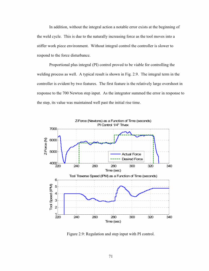
71

In addition, without the integral action a notable error exists at the beginning of

the weld cycle. This is due to the naturally increasing force as the tool moves into a

stiffer work piece environment. Without integral control the controller is slower to

respond to the force disturbance.

Proportional plus integral (PI) control proved to be viable for controlling the

welding process as well. A typical result is shown in Fig. 2.9. The integral term in the

controller is evident by two features. The first feature is the relatively large overshoot in

response to the 700 Newton step input. As the integrator summed the error in response to

the step, its value was maintained well past the initial rise time.

220 240 260 280 300 320 3404000

5000

6000

7000

Z-Force (Newtons) as a Function of Time (seconds)

PI Control 1/4" Trivex

Z-Force (N)

Time (sec)

220 240 260 280 300 320 3401

2

3

4

5

6Tool Traverse Speed (IPM) as a Function of Time (seconds)

Tool Speed (IPM)

Time (sec)

Actual Force

Desired Force

Figure 2.9: Regulation and step input with PI control.

72

The second noticeable feature of the system under PI control is the lack of steady

state error. At the time the force controller was engaged the force was naturally rising.

The system under PI responded to this error slightly faster than under P control.

However, due to the integral term an overcorrection in force occurred. Similar to the step

response the oscillation dies out and stability is maintained.

220 240 260 280 300 320 3404000

5000

6000

7000

Z-Force (Newtons) as a Function of Time (seconds)

PD Control 1/4" Trivex

Z-Force (N)

Time (sec)

220 240 260 280 300 320 3400

2

4

6Commanded Tool Traverse Speed (IPM) as a Function of Time (seconds)

Tool Speed (IPM)

Time (sec)

Actual Force

Desired Force

Figure 2.10: Regulation and step input with PD control.

When proportional plus derivative control (PD) is applied, excellent

controllability results. Fig. 2.10 shows the systems response to regulation and a step

input while under PD control. The derivative term in the control law anticipates force

overshoot and implements a correction before the overshoot occurs. As evident in Fig.

73

2.10, the systems closed loop response to a step input exhibits first order characteristics.

When compared to other controllers previously presented, the PD controller tends to

provide a more stable and smooth response.

As previously stated, the system’s dynamics are unknown with the exception of

the controller. Using the results from the P, PI, PD and PID version of the controller, it is

possible to model the dynamics of the system in response to the step input. Since the

results are the responses of the closed loop system, the challenge is to determine the feed

forward transfer function of the system.

From the results presented in Fig. 2.7 through Fig. 2.10, it can be observed how

each of control variations changes the closed loop response. From a mathematical

standpoint the P control architecture alters the feed forward transfer function the least. It

simply increases the magnitude of the numerator. Upon review of the closed response to

P control, the system tends to behave as a second order system. Assuming the system is

an ideal second order system, its closed loop response will take the form shown in Eq.

(2.3). In Eq. (2.3), ωn is the systems natural frequency, ζ is the systems damping ratio,

and s is the complex variable. From the closed-loop equation the feed forward equation

is derived to be of the form listed in Eq. (2.4). The block diagram shown in Fig. 2.3

illustrates the systems and the unknowns that had to be determined.

ωn2 / (s2 + 2ζωns + ωn

2) (2.3)

ωn2 / (s(s + 2ζωn)) (2.4)

74

From the results shown in Fig. 2.8, the amount of overshoot, peak time, and rise

time were measured. With these two measurements and treating the response as an ideal

second order system, estimates can be made for the natural frequency, damped frequency,

and the damping coefficients. In addition, the step input of 700 Newtons had to be

treated as unit step in order to obtain the proper value for the overshoot. Thus the value

of overshoot shown in Fig. 2.8 was normalized in order to obtain an equivalent overshoot

in response to a unit step. With the calculated transfer function’s coefficients a Simulink

model was constructed to validate the accuracy of the model. The Simulink model was

constructed with two feed forward transfer functions. One of the transfer functions was

for the known force controller and the other for the estimated portion of the system.

To fully validate the system the controller was changed to PID, PI, and PD for the

various tests in order to compare to the experimentally obtained results. Since the

estimated feed forward transfer was based upon an ideal second order system, initially

only the P control system fit the model. To match the other control architectures the

transfer function had to have the addition of a zero, thus increasing the order of the

system. With the addition of the zero, the coefficients of the transfer function were

readjusted by best fitting techniques. The completed Simulink model of the system is

shown in Fig. 2.11. The transient response of the system, not including the PID

controller, was model by the transfer equation given in Eq. (2.5). In Eq. (2.5), F(s) is the

output force and R(s) is the reference input force.

F(s) / R(s) = ((0.111s + 0.111) / (1.8s2 + 0.502)) e-s (2.5)

75

Figure 2.11: Simulink model of the FSW force control system.

270 275 280 285 290 295 300 305 310 315 3205000

5200

5400

5600

5800

6000

6200

6400

6600

6800

7000

Z-Force (Newtons) as a Function of Time (seconds)

P Control 1/4" Trivex Tool

Z-Force (N)

Time (sec)

Actual Force

Desired Force

Modeled Force

270 275 280 285 290 295 300 305 310 315 3205000

5200

5400

5600

5800

6000

6200

6400

6600

6800

7000

Z-Force (Newtons) as a Function of Time (seconds)

P D Control 1/4" Trivex Tool

Z-Force (N)

Time (sec)

Actual Force

Desired Force

Modeled Force

270 275 280 285 290 295 300 305 310 315 3205000

5200

5400

5600

5800

6000

6200

6400

6600

6800

7000

Z-Force (Newtons) as a Function of Time (seconds)

P I Control 1/4" Trivex Tool

Z-Force (N)

Time (sec)

Actual Force

Desired Force

Modeled Force

270 275 280 285 290 295 300 305 310 315 3204500

5000

5500

6000

6500

Z-Force (Newtons) as a Function of Time (seconds)

P I D Control 1/4" Trivex Tool

Z-Force (N)

Time (sec)

Actual Force

Desired Force

Modeled Force

Figure 2.12: Results of the modeled transient response of the FSW force control system.

The results of the model are shown on Fig. 2.12. In each of the tests, a

comparison was made to the experimentally obtained results. The model provided results

that correlated well with the experimentally obtained results for all the control

architectures.

76

As a final validation of the force control architecture to produce good welds,

macro sectioning of welds were performed. As with any manufacturing process and

system, validating the ability of the system to produce a good product is essential. Thus

these tests were performed to see if the changing of the traverse speed during the weld

cycle affected the quality of the welds in a negative manner.

Figure 2.13 and Fig. 2.14 are the etched macro sections of two different welds

subjected to step inputs. The weld cross section shown in Fig. 2.13 was produced using

the ¼ inch (6.35 mm) Trivex tool while the weld shown in Fig. 2.14 was produced using

the ¼ inch (6.35 mm) threaded tool.

As can be seen in the figures, no evidence of worm holes or internal voids were

seen in the cross sections. All welds were found to acceptable. From the cross sections,

the weld nuggets are clearly visible due to their refined grain structures. In comparison to

the unaffected parent metal the weld nuggets grain structure appears to be more refined.

This is further evidenced by the small internal voids that are present in the unaffected

parent metal. These small voids in the unaffected parent metal and can been seen near

the right edge of Fig. 2.13 and Fig. 2.14.

Figure 2.13: Weld using ¼ inch Trivex tool and force control via traverse speed.

77

Figure 2.14: Weld using ¼ inch threaded tool and force control via traverse speed.

Although acceptable, both welds had a small amount of weld flash deposited on

the retreating side of the weld surface. Since the tool’s vertical position is fixed, a robust

plunge depth must be set in order to insure the tool’s shoulder remains in contact with the

parent metal. As with any stock material, there are variations in the materials

dimensions. This was the case in this experiment as well. Plunge depth of the trailing

edge of the tool’s shoulder was set at 0.001 inches (0.0254 mm). Although a small

amount of flash was generated no surface gouging or negative effects were found in the

welds.

Upon closer examination of the weld nuggets, more stirring is evident with the

threaded tool than with the Trivex. The threads were designed to push metal down into

the lower region of the weld nuggets and help prevent internal voids from forming in this

region. When comparing the results in Fig. 2.13 and Fig. 2.14, the weld nugget for the

threaded tool is wider and appears to have been stirred more. Furthermore a small root

flaw is just beginning to form at the bottom surface of the weld produced with the Trivex

tool. This root flaw is further evidence of reducing stirring in this region.

Another interesting observation is how the axial force correlates with the relative

temperature of the welding environment. In essence the axial force is an excellent

78

indicator of temperature underneath the tool’s shoulder. Although the axial force cannot

yet be used to obtain an accurate reading of the temperature, it can provide information

on the relative temperature as the weld process proceeds. This can be seen in the base

line weld shown in Fig. 2.4. As the tool moved away from its plunge point where a lot of

heating occurred, it entered into a colder region within the work piece. When this

occurred the axial force increased. When the tool moved near the end of the work piece,

heat began to build up within the localized end region of the work piece and the axial

force decreased.

Since axial force is used as the control feedback signal for the force controller, a

constant welding temperature is trying to be maintained by the controller. Hence it can

be concluded that not only does the force controller produce a desired force, but it also

controls the heat distribution into the weld seam. This hypothesis of heat distribution

control can be supported with results of Schmidt and Hattel (2008) in which they describe

a thermal model of FSW. They presented Eq. (2.5) describing the total heat generation

Qtotal.

Qtotal = δQsticking + (1-δ)Qsliding

= 2/3πω[δτyield + (1-δ)µp][(R3shoulder – R

3probe)(1-tan α) + R

3probe + 3R

2probeHprobe] (2.5)

In this equation by Schmidt and Hattel, the variable δ is the contact state variable

or dimensionless slip rate, τyield is the yield stress of the work piece material at the

welding temperature, µ is the coefficient of friction, p is the contact interface pressure, ω

is the angular rotation velocity, α is the cone angle of the tool’s pin, Rshoulder is the

79

shoulder radius of the tool, Rprobe is the radius of the tool’s pin, and lastly, Hprobe is the

height of the tool’s pin. Schmidt and Hattel go on to note the typical expression for a

numerical model is in the form of a position dependent surface flux qtotal. The units of the

model take the form of power per unit area. In its final form the heat generation model

can be expressed as Eq. (2.6), which is a radius dependant surface flux. The simplified

equation assumes tool geometry of only a flat shoulder.

qtotal = (3Qtotalr) / (2πR3shoulder) (2.6)

For the hypothesis of heat distribution to be true, qtotal must be constant

throughout the force controlled welding process. Upon review of the variables in Eq.

(2.5) and Eq. (2.6), it can be hypothesized that they all become constant when force

control via traverse speed is employed and a few assumptions regarding force control are

taken into account. First, the plunge depth is constant and does not change as the tool

traverses the work piece. Second, the work piece material properties and thickness is

constant throughout. Third, a constant axial force produces a constant contact pressure at

the interface. Fourth, a constant axial force and a constant plunge depth lead to the other

forces acting at interface, such as torque and traverse force, to be constant as well.

If the force controller maintains a constant axial force, is the average temperature

in the work piece beneath the tool constant as well? With a constant temperature the

localized yield strength of the work piece will also maintain a constant value. In

addition, the constant pressure, temperature, and interface surface area, should lead to a

constant slip rate.

80

With all of these variables being constant due to force control, a constant rate of

heat generation should exist. Notice that the rate of heat generation is not a function of

traverse rate. Thus, as the tool traverses along the weld seam at varying speeds, the rate

of heat generation is assumed to be the same at any speed. With the force controller

varying the traverse speeds, a variable amount of heat is deposited per unit length along

the weld seam. The intelligence of the control system measures the relative temperature

beneath the tool through axial force and then adjusts the amount of heat being deposited

into the weld seam directly beneath the tool by changing the tool’s traverse rate. By

doing this the controller distributes heat as it is needed to maintain a constant welding

temperature along the entire weld seam.

Force Control: Traverse Speed vs Weld Temperature

4

6

8

10

12

14

16

250 300 350 400 450 500 550 600

Weld Temperature (K)

Average Steady-State Traverse Speed (ipm)

Figure 2.15: FSW preheating experiments under force control.

Sinclair (2009) used this force control architecture to analyze the resulting steady

state traverse speed when the work piece was preheated to a desired temperature. His

81

results are shown in Fig. 2.15. Under the force control algorithm the FSW tool traversed

faster when higher preheating temperatures were used.

For his experiments, Sinclair used a ¼ inch (6.35 mm) Trivex tool and set the

desired axial force at 4000 Newtons. As the work piece was preheated to an elevated

temperature, there was less need for process generated heat to soften the work piece.

Even though the tool was generating heat at a constant rate, it was being distributed in a

manner proportional to the traverse rate. As the preheat temperature was increased for

each test, the resulting tool traverse speed increased since less generated heat was needed

beneath the tool. These results support the hypothesis that heat control is obtained as a

byproduct when force control is utilized with traverse speed as the controlling variable.

Conclusions

Based upon these presented results, it can be concluded that using traverse speed

instead of plunge depth as the controlling variable, provides much greater accuracy in

maintaining a desired axial force. There are two key enablers for this controllability

advantage. The first enabler is the unidirectional dynamics of the drive motor. The

traverse motor never has to reverse its direction. It just simply changes speed. Without

having to stop and reverse itself, greater bandwidth and response times are achieved as

compared to a motor controlling the plunge depth. The second enabler is load dynamics.

The traverse axis of the machine does not support the axial load, thus the drive system is

not burdened by being subjected to the changing load it is trying to control. Although the

traverse force does trend with the axial force, its magnitude is substantially less. The

drive motor and its VFD are free of the large dynamic forces. When compared to the

82

axial drive system, the axial motor has to stop its motion and change its direction

frequently. It is also taxed with the dynamic loading. These two items lead to lower

bandwidth and reaction times. In addition, the drive system must be able to support the

larger axial load which requires either greater gear reduction, or a larger drive motor,

either of which contribute to the disadvantage of using plunge depth as the controlling

variable.

The conclusion that axial force control via traverse speed is better depends upon

the equipment being used and the process setup. The welding experiments conducted at

Vanderbilt University were conducted on a three axis milling machine. Each axis was

controlled independently and aligned with a Cartesian reference frame. Due to a constant

plunge depth, the worktable was fixed along the vertical axis during the welding

operation. Table movement was only needed along the traverse axis while the force

controller was active. In addition the force control loop resided outside the position

control loop. The same results might not be achieved using certain types of robots. For

instance if a six axis jointed-arm robot is to control axial force via traverse speed, more

than one linkage must be adjusted simultaneously as the tool continuously traverses along

the weld seam. Any simultaneous multi linkage adjustment possibly could result in small

fluctuations in the tool’s plunge depth. This will further lead to fluctuations in the axial

force and possibly negating the advantages of using traverse speed as the controlling

variable. For force control via traverse speed to be successful there can not be any

linkage adjustment perpendicular to the weld seam. In summary, the vertical position of

the tool can not change relative to the position of the work piece surface. The robot must

be capable of maintaining noncompliance along the FSW tool’s vertical axis. This force

83

control method probably would work best when the robot’s linkages to be adjusted reside

in a parallel plane to the weld seam. The linkages could be adjusted via either prismatic

or revolute joints. Thus a selectively compliant assembly robot arm (SCARA), a

Cartesian robot or a gantry style machine tool would be a good candidate for supporting

force control via traverse speed. Of course this is valid provided that the robot or

machine is capable of the supporting the high loads associated with FSW.

Process setup also requires the condition of the welding surface to be relatively

constant. With the controlling variable of traverse speed, there is no means to adjust the

vertical position of the tool to changing surface conditions. This requires the plunge

depth of the tool to be set to a position such that the tool’s shoulder will always be in

contact with the material. Essentially the plunge depth must be set as if the welding was

being conducted under position control.

Upon further review of the experimentally obtained results it is interesting to note

how the traverse speed of the tool is continuously adjusted to maintain the desired force.

It can clearly be seen that the axial force increases as the tool traverses at a faster rate and

decreases as the tool traverses at a slower rate. These results are in agreement with the

findings of Cook et al. (2003). From the results shown in Fig. 2.6 through Fig. 2.10, it

can be concluded as the FSW tool’s traverse velocity increases, less process generated

heat is deposited per unit length of weld. With less heat being deposited into a unit

volume of weld zone material directly beneath the tool, cooler welding conditions

emerge. With cooler welding conditions, the work piece becomes stiffer which results in

higher welding forces. The opposite reaction occurs when the tool slows down. As the

traverse velocity decreases, more process generated heat is deposited per unit length into

84

the weld seam. With this increased heat, the welding forces are lower due to the softer

environment.

Future work can be done to verify the concept of heat control. How accurately is

the welding temperature being controlled? This is a major question yet to be answered

regarding the hypothesis of heat control. When Sinclair measured the tool’s temperature

during each of the tests shown in Fig. 2.15, he found the results to be identical no mater

what the preheating temperature of the work piece was. In each case the maximum tool

temperature reached was 333° C. These results warrant further investigation, but thus far

they support the idea of heat control. With force and heat control of FSW welding,

optimum process condition would result. This means the intelligence of the controller

working in conjunction with the machinery, not only would produce a quality weld, but it

would produce it with the most efficient speed. The system would naturally insure that

adequate heating and force are present in the welding environment beneath the tool.

Along with the investigation of heat control, further modeling work can be done

to breakdown the presented transfer function into process and equipment components.

The feed forward transfer function models the traverse drive system and the welding

process. With this model refinement, more insight would be gained about the welding

process itself. In addition more advanced control algorithms could be developed for

force control.

85

CHAPTER III

THE IDENTIFICATION OF THE KEY ENABLERS FOR FORCE CONTROL OF FRICTION STIR WELDING

William R. Longhurst, Alvin M. Strauss, George E. Cook

American Society of Mechanical Engineers Journal of Manufacturing Science and

Engineering. Current Status: Submitted June 10, 2009. Under Review.

Abstract

The process requires a large axial force to be maintained on the tool. Force

control is needed in robotic friction stir welding (FSW) processes to compensate for the

compliant nature of robots. Without force control, welding flaws would continuously

emerge as the robot repositioned its linkages to traverse the tool along the intended weld

seam. Insufficient plunge depth would result and cause the welding flaws as the robot’s

linkages yielded from the resulting force in welding environment.

As FSW continues to emerge in manufacturing, robotic applications will be

desired to establish flexible automation. The research presented here identifies the key

enablers for successful and stable force control of FSW. To this end, a FSW force

controller was designed and implemented on a retrofitted Milwaukee Model K milling

machine. The closed loop proportional, integral plus derivative (PID) control

architecture was tuned using the Ziegler-Nichols method. Welding experiments were

86

conducted by butt welding 0.25 inch (6.35 mm) x 1.50 inch (38.1 mm) x 8.0 inch (203.2

mm) samples of aluminum 6061 with a 0.25 inch (6.35 mm) threaded tool.

The experimental force control system was able to regulate to a desired force with

a standard deviation of 129.4 Newtons. From the experiments, it was determined that

tool geometry and position are important parameters influencing the performance of the

force controller, and four key enablers were identified for stable force control of FSW.

The most important enabler is the maintaining of the position of a portion of the tool’s

shoulder above the work piece surface. When the shoulder is completely submerged

below the surface, an unstable system occurs. The other key enablers are a smooth

motion profile, an increased lead angle, and positional constraints for the tool. These last

three enablers contribute to the stability of the system by making the tool’s interaction

with the nonlinear welding environment less sensitive.

It is concluded that successful implementation of force control in robotic FSW

systems, can be obtained by establishing and adhering to these key enablers. In addition,

force control via plunge depth adjustment reduces weld flash and improves the

appearance of the weld.

Introduction

Friction Stir Welding (FSW) is a solid state material joining process. The process

involves plunging a rotating tool into the parent metals that define the work piece. The

rotating tool consists of a shoulder and a pin (or probe) that is used to plastically

deformed the parent metals and then forge them together into a single piece of material.

As the tool rotates and traverses along the joint line to be welded, it shears a thin layer of

87

material from the parent metals and then rotates the materials to the backside of the pin.

While at the backside, the severely deformed materials are consolidated under the forging

pressure of the shoulder. Heat generated through plastic deformation and friction softens

the work piece and aids in the joining process by reducing the resulting forces.

FSW is emerging as a viable technology in the fields of manufacturing and

product development. Successful applications of the joining of various alloys have made

FSW an attractive technology for the aerospace and automotive industries. The current

state of FSW technology restricts its usage due to process limitations, equipment

requirements, capital investments and a lack of full understanding of the physical joining

process.

As FSW technology began to mature during the late 1990s, robot applications

became apparent. Similar to other welding technologies, the application of FSW through

robotics provides a very flexible platform for automation. However, with FSW the

relatively large forces present a challenge. Robots are limited by the magnitude of the

load they are able to support at their face plates. In addition, their compliant nature

makes FSW much more challenging. To address the compliance problem, force control

has been presented as a solution. With robotic FSW the challenge is to keep the tool

positioned correctly while the linkages of the robot continually reposition themselves.

The motion of the linkages along with the large forces acting at the face plate results in

tool positioning errors. Along with these positioning errors, large fluctuations in axial

force result. These positioning errors and force fluctuations will lead to insufficient

deformation, forging and consolidation of the parent metals.

88

Cook et al. (2004) (2003) stated force control is the key to controlling robotic

FSW. They performed an in-depth study of how the axial force changes as a function of

process parameters. They determined that maintaining position control of the tool

relative to the work piece is too difficult, and that force control is a much more robust

control strategy for robotic applications of FSW. Another conclusion drawn by their

work is that the indentation characteristics of the tool, as it moves downward into the

work piece, is ill behaved and could cause closed-loop instability. They note how a small

amount of change in the vertical position of the tool, while in contact with the work

piece, produces large changes in the axial force. The shape of this response varies under

different process conditions such as rotation speed. Lastly, they note how the force tends

to return to its initial value after the tool has plunged deeper into the work piece. They

conclude that no significant increase in force occurs, other than the initial transient.

Notice how the force spikes as a result of small step inputs. In addition notice how the

force slowly subsides back near its original value prior to the increase in plunge depth.

Successful applications of robotic FSW have been documented with work by

Smith (2000), Soron and Kalaykov (2006), and Zhao et al. (2007). They all developed

and implemented a force control architecture using plunge depth as the controlling

variable. They were able to conclude that it was feasible to implement FSW force control

architectures. However, using plunge depth as the controlling variable did present

several challenges. Soron and Kalaykov concluded that even with the added force

control to the robotic FSW system, axial force oscillations exist when the tool makes

contact with the material. They also note the penetration depth is hard to predict due to

the positioning error of the robot. Zhao et al. presented a non-linear axial force controller

89

they developed and implemented for a FSW process. They were able to experimentally

characterize the static and dynamic behavior of the interaction between the FSW tool and

the work piece. With this information and using an open architecture control system they

were able to design a controller using Polynomial Pole Placement. Good results were

obtained, but to handle the non-linear transient response when the tool’s plunge depth

changed, the control system had to incorporate experimentally obtained dynamic

parameters. Thus, the open architecture of the control platform was needed in order to

implement this force controller. Plus, the controller parameters were specific to their

experimental setup.

Even with these advances the problems associated with robotic FSW remain open.

As noted by Soron and Kalaykov, problems still exists with force oscillations. The

highly non-linear aspect of the welding environment makes it extremely difficult to

implement a robust system that maintains stability over a large range of process

configurations and parameters. The papers cited above report successful

implementations of robotic FSW systems, but they do not state in detail why they were

successful.

The goal of this research was to build a FSW force controller and identify key

enablers of the system so that efficient and successful implementations can be performed

in the future. These key enablers specifically address stability issues associated with

varying plunge depth. It was concluded that tool geometry and tool position relative to

the work piece play an important role in maintaining stability of the system. In addition,

a comparison is drawn to other force control systems that utilize plunge depth as the

90

controlling variable. Recommendations are made regarding automatic machinery

configurations.

Experimental Setup

The experiment was conducted on the FSW system at Vanderbilt University. The

FSW system is a Milwaukee Model K milling machine that has been retrofitted with

more advanced motors and instrumentation. The system is shown in Fig. 3.1. These

retrofits were previously added to automate the system and provide a programmable

platform for FSW experimentation. At the top of the control hierarchy is a master

computer that enables all of the systems subcomponents such as the motor drive

controllers and instrumentation. The master computer is a Dell Precision 340 that uses

Microsoft Windows XP as its operating system. The welding and force control code was

written in C#. A graphical user interface within the C# software allows the operator to

select the desired welding parameters for the pending operation. These parameters

include the FSW tool’s rotation speed, traverse speed, plunge depth and weld path

position.

The tool’s vertical axis coincides with the milling machine worktable’s vertical

axis when the tool is at a zero degree tilt angle. The worktable resides on the knee that is

mounted to a vertical positioning screw and secured in sliding dovetail joints. The knee

travels on the screw via a gear system inside the knee. An externally mounted belt and

pulley system is attached to the input shaft of the gear system. Power is provided by a

Parker Compumoter KH series brushless servo motor. The servo motor is controlled by a

Parker Compumotor KHX-250 servo drive that utilizes a proportional, integral plus

91

derivative (PID) control algorithm. Command signals are sent directly from the master

computer to the servo drive. Vertical position of the table is obtained from a Reinshaw

linear scale that has a resolution of 10 micrometers (0.0004 inches). Position data from

the sensor is feed into a sensor box were it is converted to a digital signal prior to being

sent to the master computer.

Figure 3.1: FSW machine at Vanderbilt University.

Welding force data is collected through a Kistler Rotating Cutting Force

Dynamometer. The dynamometer collects x-axis force, y-axis force, z-axis force as well

as the torque about the z-axis. The analog signal from the dynamometer is sent to a signal

conditioning box were it is converted from an analog signal to a digital signal. Once

converted the data is sent to a separate computer where the data is sorted, recorded and

displayed before being sent to the master computer.

An overview of the closed loop force control system is illustrated in the control

block diagram of Fig. 3.2. Within the master computer a desired z force is selected. The

92

desired force value is subtracted from the actual z force value to obtain a force error. The

force error signal is then processed in the control law. The resulting processed control

signal is then multiplied by a factor of 0.09 to translate the signal from Newtons of force

to a desired rate of change in the servo motor’s shaft. The servo drive produces a change

in the vertical position of the tool which results in a change the of z force in the welding

environment. The dynamometer reads the resulting force and returns it to the master

computer where it is once again compared to the reference signal.

Figure 3.2: Block diagram of force control via plunge depth.

The servo motor has two modes in which it can operate. The servo motor can

move its output shaft to a desired position or it can turn the output shaft at a desired

speed. In addition to the mode selection, velocity and acceleration profiles were

preprogrammed for complete motion control of the output shaft and the movement of the

FSW tool.

The measured z force signal was very noisy. This noise makes the process of

applying derivative control to the system very difficult. The noise would simply be

93

amplified by the controller. To address this problem, a filter was implemented. The filter

is a five point moving average of the z force with an interrupt frequency of 3.33 Hz. For

this experimental setup these filter parameters were found to provide adequate noise

reduction without adding too much phase lag in the signal.

The force control law consisted of PID control. Due to the retrofitted nature of

the FSW system there are several unknown parameters that could not be accurately

modeled to create a non-linear modeled based control system. For instance, the force

control loop resides outside the control loop for the vertical drive system. The Parker

Compumotor drive and servo motor uses its own proprietary control techniques to drive

the motor. Thus, obtaining the parameters of the controller as well the physical

parameters of the motor, belt drive, and power screw would require an extensive amount

of testing and analysis. In addition, the time needed for signal processing and

transmission through the master computer, dynamometer, sensor box and the servo would

also have to be experimentally determined. With all of these variables to consider the

potential performance of a model based controller might not be much better than a

standard PID controller. For this study to create and investigate the performance of z axis

force control via plunge depth, PID control architecture was chosen as the best option.

To address the transport delay between the initiation of the control signal and the change

in force, a simple delay of 1 second in the control update time was utilized. The 1 second

delay allowed the FSW tool to change position and a change in z force to occur. The

delay in control signal update proved to be effective without the need of adding a more

complicated controls approach such as a Smith Predictor-Corrector (Ogata 2002).

94

To tune the PID force controller and achieve optimum control, the Ziegler-

Nichols tuning method was used (Ogata 2002). The Ziegler-Nichols tuning method

called for the controller to use only proportional gain while welding. While using

proportion control only, a critical gain value was experimentally determined through trial

and error. Over the course of several welds, the gain was steadily increased until the

resulting z force achieved sustained oscillation. The sustained oscillation constituted

marginally stable behavior. The resulting control gain and time period between

oscillations was recorded and used to calculate PID gains for the controller. The

resulting PID control law is shown in Eq. (3.1). In Eq. (3.1), Kp is the proportional gain,

Ki is the integral gain, Kd is the derivative gain, e is the error and u is the resulting control

signal as a function of time t.

Kp e + Ki ∫e + Kd e΄ = u(t) (3.1)

For this force control research, experiments using two different FSW tools were

performed. The two tools with their contrasting size and geometry provided insight into

the dynamics of the FSW system. The first tool consisted of a slightly undersized 0.25

inch (6.35 mm) Trivex pin with a flat 0.625 inch (15.875 mm) diameter shoulder. The

Trivex profile geometry is similar to an equilateral triangle, but with its edge surfaces

slightly convex. The pin with its Trivex geometry was 0.235 inches (5.969 mm) long by

0.210 inches (5.334 mm) across its widest point. The second tool was larger in size as

compared to the 0.25 inch (6.35 mm) Trivex. The second tool consisted of a 0.25 inch

(6.35 mm) threaded pin. The threaded pin was 0.235 inches (5.969 mm) long with a

95

diameter of 0.250 inches (6.35 mm) across its threads. The shoulder was of a hybrid

nature. It had a flat 0.625 inch (15.875 mm) diameter shoulder that acted as the forging

surface. The remaining portion of the shoulder was on a 7° taper that started at the 0.625

inch (15.875 mm) diameter point and continued to the 1.0 inch (25.4 mm) outermost

diameter. The tools are shown in Fig. 3.3.

Figure 3.3: Trivex and threaded FSW tool.

Using the Ziegler-Nichols tuning method, critical gains were determined for both

tools. The critical gain and period for the 0.25 inch (6.35 mm) Trivex tool was 3.5 and

13 seconds respectively. The critical gain and period for the 0.25 inch (6.35 mm)

threaded tool was 4.14 and 7.5 seconds respectively. The resulting control gains are

shown in Table 3.1.

Table 3.1: Plunge Depth Mode Force Control Gains.

96

For the experiment 0.625 inch (6.35 mm) butt welding with full penetration was

performed. The material used was aluminum 6061. The work piece consisted of two

0.25 inch (6.35 mm) by 1.50 inch (38.1 mm) by 8.0 inch (203.2 mm) long samples. Each

weld began with the tool plunging into the metal 1.0 inch (25.4 mm) from the end of the

work piece. Once the tool achieved the desired plunge depth it dwelled at that location

for 5 seconds in order to soften the work piece by generating additional heat. After

dwelling, the tool began to traverse forward at 6 inches per minute (IPM) (152.4 mm per

min.). After traversing 1 inch (25.4 mm) the force controller was engaged. The force

controller was operating in a regulation mode, meaning whatever the z force was at the

time of engagement, was the selected desired force. The system operated under force

control mode until it reached 1 inch (25.4 mm) from the end of the 8 inch (203.2 mm)

work piece. Thus 5 inches (127.0 mm) of welding was conducted each time under force

control. For many of the welds a step input in desired force occurred after 2 inches (50.8

mm) of regulation. Each step input was of 1000 Newtons in magnitudes. For every weld

made, the tool’s shoulder was initially plunged between 0.000 – 0.002 inches (0.0508

mm) below the surface and the tool’s rotation rate was maintained at a constant 1400

revolutions per minute (RPM).

To provide a base line of the welding environment, a weld was made without any

force control using the 0.25 inch (6.35 mm) Trivex tool. The results are shown in Fig.

3.4. The resulting force during the initial tool plunge into the work piece is identified on

the figure as the pin plunge and shoulder plunge regions. After the tool has plunged and

dwelled for 5 seconds, the forward motion of the tool begins. This point is easily

97

identified as the sharp increase in force after the shoulder plunge and dwell period. After

1.0 inch (25.4 mm) of forward travel the force controller is normally engaged at this

point. However, for this base line sample the force controller is not engaged, but the

force occurring at the engagement point is displayed as a desired force reference. From

the base line sample it can clearly be seen that the z force continues to increase about two

thirds of the distance across the weld seam. The increase is due to the tool moving into

un-welded and colder material. This also indicates the welding process has not yet

reached a steady state.

100 120 140 160 180 200 220 240 260 280 3000

1000

2000

3000

4000

5000

6000

7000

8000Z-Force (Newtons) as a Function of Time (seconds)

Z-Force (N)

Time (sec)

Actual Z Force

Desired Z Force

Pin Plunge

Shoulder Plunge

Weld

Force

Control

Start/Stop

Zone

Traverse Forward

Figure 3.4: Weld sample with no force control.

98

Results and Discussion

Initial observation of the system’s performance leads to the identification of the

important configurations necessary for stable control. The highly nonlinear welding

environment and the tight coupling of the axial force to the process parameters as well as

the thermal conditions dictate the need for robustness. To achieve this robustness,

specific process configurations must be realized and correctly implemented. These

configurations include the tool’s position relative to the work piece, the geometry of the

tool and its dynamic characteristics. Without properly addressing these issues, instability

will result. The parameters were identified through numerous tests and analytical

reasoning. The requirement to establish these conditions holds true for both robotic and

machine tool applications.

As the tool was either plunged further or retracted slightly from the work piece a

rather large transient force was observed. This force response can be characterized as

viscous in nature. In other words it was proportional to the velocity of the FSW tool.

Since the welding environment is rather stiff, any movement in the tool will generate a

large change in force. As the tool began to move, the force quickly increased (or

decreased) causing the error signal in the force control to quickly reach a value of zero

and thus stopping further motion of the tool. However once the force was achieved, it

began to dissipate back to its original value. This was true for both plunging and

retracting motions. These transient forces proved to be taxing on the control system. The

controller was constantly starting and stopping the motor. More importantly the

generated force change was a result of the tool’s velocity and not its position relative to

the work piece.

99

Smother tool motion was found to reduce the transient effect. Although the

sudden change in force can not be eliminated, it can be reduced in magnitude. A

reduction in magnitude produces a feedback signal to the force controller that is more

representative of the tool depth into the work piece than its velocity. Tool plunge depth

is more important than vertical velocity in producing a quality weld. The tool’s shoulder

must be in contact with the work piece in order for the plasticized material to be forged

together on the backside of the pin. During the early phases of force controlled welding,

it was observed that an adequate z force can be generated while an inadequate amount of

shoulder contact is present. This occurs when the shoulder disengages from the work

piece and the z force does not drop significantly due to the highly nonlinear environment.

When this happened the force sensor could not distinguish between a force being applied

on the pin and the force on the shoulder.

With a reduction in the transient force, the force controller can more efficiently

use the z axis servo motor. The change in force becomes more of a function of tool

position and less of a function of tool velocity. Since the force is more indicative of

position, the z axis motor is not as taxed. The motor does not undergo as many on - off

cycles to drive the tool to its required position.

The z axis servo motor on the FSW system at Vanderbilt University has two

modes of operation. One is a discrete mode and the other is a continuous mode. The

discrete mode turns the motor’s shaft to a desired position under a desired acceleration

and velocity. In the continuous mode the shaft turns at a desired velocity until it receives

a stop command. In both modes, motion profiles establishing the acceleration and

velocity are entered as part of the input command.

100

Due to the highly nonlinear welding environment, the continuous mode was found

to produce better results. To operate over a wide range of parameters, the discrete mode

required the force controller to know how much to adjust the plunge depth. Although the

plunge depth will change proportionally to the force error, changing thermal conditions

within the work piece will change the amount of force produced by a unit change in

plunge depth. Thus a tuned controller would have a narrow range of process parameters

for optimum performance. The amount of time to eliminate the force error will take

longer due to the nature of the incremental changes in plunge depth. By using the

continuous mode, the force controller has a much larger range for optimum performance.

In the continuous mode the servo motor adjusts the plunge depth until the force controller

tells it to stop. It is told to stop when the force error has returned to zero. By using the

continuous mode of operation, much faster response time in eliminating force error is

experienced.

The motion profile shown in Fig. 3.5 was found to work well for the FSW force

control system established at Vanderbilt University. The magnitude of the acceleration

and velocity is scaled to the size of the processed error signal. The amount of time for

the acceleration and deceleration was preset at 0.2 seconds. This value was found to be

adequate for this system. When selecting the acceleration time for future systems, a

compromise must be made between response time and reduction of the transient force

response. A longer acceleration will lead to a slower response and a larger amount of

error. Along with the acceleration, a long deceleration will cause a force overshoot. In

contrast, a large change in acceleration over a short period of time will cause a jerk

101

action, which will result in a larger transient force. The key enabler is to create smooth

motion while maintaining an adequate response time.

Figure 3.5: Servo motor motion profile.

As mentioned above, it was observed while welding under force control, the

shoulder disengaging from the work piece while the axial force still remained near a

constant value. This is possible because once the shoulder is removed from the work

piece, less heat is generated in the welding environment. With less heat, the work piece

becomes stiffer. With just the pin plunged into the stiffer work piece, the same amount of

force can result as when the shoulder is plunged into a softer work piece. A method to

prevent this control issue is to constrain the plunge depth.

Adding constrains to the plunge depth induces an element of positional control

into the system. This is easily accomplished by monitoring the position of the tool

relative to the work piece and then restricting its motion from going beyond the constraint

boundaries. Adding constraints does not completely prevent the shoulder from

102

disengaging from the work piece in all cases. When the constraint boundary is

established it must be at the maximum height of the work piece. The maximum height

might not always be accurately known because of material thickness variation. In

addition, when the work piece’s thickness is at its minimum condition, it still will be

possible for the shoulder to disengage from the work piece.

Only a very small amount of plunge depth is needed to produce a quality weld.

Hence there is a very narrow range of vertical travel between a quality weld and a no

weld condition. Excellent welds were produced with plunge depths of only 0.000 to

0.002 inches (0.000 to 0.0508 mm). These shallow plunge depths were possible due to

the initial plunge of the tool into the work piece. As the tool plunged, material was

extruded upward along the pin and onto the surface of the shoulder, thereby creating a

layer of material between the shoulder and the work piece prior to the backside of the

shoulder reaching the nominal height of the work piece. Deeper plunge depths can be

obtained but undesirable weld flash is generated. The presence of weld flash means less

material is in the weld joint which reduces its load bearing capability. In addition, if the

weld seam needs to be cosmetically pleasing, some type of flash removal operation must

be preformed after welding. Thus careful planning and control of the plunge depth will

make a manufacturing operation more efficient.

Constraining the maximum amount of plunge depth is also beneficial. It was also

observed than during very hot welding conditions the tool would continue to plunge into

the work piece without a significant amount of force increase. If the tool continues to

plunge into the work piece without an increase in force two major problems will arise.

103

The first problem is that the tool might collide with the backing anvil. Under

ideal conditions the pin must be a few thousands of an inch above the backing anvil.

With the pin rotating, material just below its bottom surface undergoes plastic

deformation and forging. It is not necessary for the tool to fully penetrate the work piece

in order to produce full penetration welds. If the tool fully penetrates, some bonding

between the work piece and the backing anvil would likely occur. Obviously, this is an

undesirable condition that must be avoided. If the pin did collide with the backing anvil,

the tool would encounter increases in load, and could fracture and damage the fixture.

This is another undesirable condition that must be avoided.

The second major problem that occurs without a constraint for maximum plunge

depth is an unstable condition will evolve once the entire shoulder is submerged below

the surface of the work piece. For force control via plunge depth to work, there must be a

change in force when the plunge depth is changed. It was discovered that the z force is

not necessarily a function of plunge depth. It is more a function of the amount of tool

surface area in contact with the work piece. As a tool is plunged into the work piece,

more of its shoulder’s surface area comes into contact with the work piece. This assumes

that the tool is on a lead angle, or the shoulder is tapered, which is typical of most

applications. With more surface area in contact with the work piece, more force occurs.

Once the shoulder is completely submerged below the surface a completely different set

of dynamics arise. As the tool continues to travel deeper, there is not a change in the

amount of shoulder surface area in contact with the work piece. Without a change in

surface area, there is not a change in force that can be related to plunge depth. The z

force overwhelming becomes a function of plunge depth velocity rather than plunge

104

depth. When the shoulder is submerged below the surface, the slightest movement of the

tool in the vertical direction produces a spike in the z force. The force continues to

increase or decrease until the force error is eliminated. For our configuration, it only

required a slight amount of tool movement for this to occur. However, as soon as the

motion stopped, the force quickly returned to near its original value. It is reasonable to

conclude that the transient nature of the force is due to material being squeezed out from

underneath the tool when the tool is plunged deeper into the work piece. The opposite

condition occurs when the tool’s plunge depth is reduced. As the tool is retracted, the

material underneath the tool relaxes due to its elastic property. The relaxation of the

material exerts less force on the tool. However, when a portion of the tool’s shoulder is

above the work piece’s surface, the change in force due to the change in tool surface area

contact with the work piece dominates the process. A much larger value of force occurs

when more surface area comes into contact with the work piece than that which occurs

when material is squeezed from beneath the tool. This is evident by the reduction in the

transient force when part of the tool’s shoulder is above the work piece’s surface. Since a

very large change in force occurs when there is a change in the amount of tool surface

area exposed to the work piece, only a small amount of tool movement is needed to

generate the change in force. A small amount of tool movement in conjunction with

smooth motion minimizes the transient spike in z force and thus adds stability to the force

controller.

Of course there is still a small relation between tool depth and z force, once the

tool’s shoulder is submerged below the surface. However, it requires such a large

amount of tool movement, it becomes impractical due to the large amount of generated

105

weld flash. As an example, when the plunge depth was started at 0.009 inches (0.2286

mm) and the tool began to traverse forward there was a natural increase in z force due to

the tool moving into a colder welding environment. As would be expected the force

controller tried to lower the z force back to the desired value by reducing the plunge

depth. As soon as the controller adjusted the plunge depth the force quickly dropped in

value and the controller stopped the motion of the tool. Soon after that, the force returned

to its prior value. The process continuously repeated itself. The force varied up and

down with virtually no sense of control being realized. After a few minutes the tool had

traveled the 0.009 inches (0.2286 mm) to the work piece’s surface. Once at the surface

the amount of the tool shoulder’s surface area exposed to the work piece changed with

each vertical motion. At that point the transient force spikes subsided and a sense of

force control emerged. The desired z force was able to be achieved and maintained once

the tool’s shoulder was at the surface.

Tool geometry was found to play an important role in the dynamic behavior of

FSW under force control. As mention above, it is vital for a portion of the tool’s

shoulder to stay above the work piece’s surface. It was discovered through the welding

experiments that different tool geometries and configurations affect the sensitivity of the

force controller. For instance the 0.25 inch (6.35 mm) Trivex tool could be configured to

create an extremely sensitive condition whereby the force controller would become

unstable or it could be configured so as to provide a robust and stable force control

platform. This was done simply by changing the lead angle of the tool.

As noted earlier the 0.25 inch (6.35 mm) Trivex tool had a flat shoulder. When

the tool was at a 0° lead angle an unstable situation occurred. Any change to the plunge

106

depth by the force controller did not produce a lasting change in z force due to a change

in shoulder surface area in contact with the work piece. The unstable situation emerged

were the z force oscillated due to the transient response.

When the tool was placed at a 1° lead angle, the process became less sensitive and

a stable condition emerged. As the tool’s plunge depth changed, so did the amount of

surface area in contact with the work piece. With the tool being on an angle, only a

portion of the shoulder was below the surface. Thus, the tool had a wider range of plunge

depths it could achieve without the controller becoming unstable. Using trigonometry, a

range of plunge depths can be estimated. With a 0.625 inch (15.875 mm) diameter

shoulder positioned at a 1° lead angle, the tool had a plunge depth range of 0.011 inches

(0.2794 mm).

The range of plunge depths can be enlarged by increasing the lead angle. This

was validated by welding with different lead angles. When the 0.25 inch (6.35 mm)

Trivex tool was at a 1° lead angle, a 1000 N step increase in force could not be obtained.

The system would simply go unstable as it tried to achieve the desired increase in force.

However, when the tool was set to 2°, no stability issues arose and the force controller

was able to achieve the desired increase.

This phenomenon can be expressed mathematically by analyzing the surface area

of the tool’s shoulder in contact with the work piece and differentiating with respect to

the plunge depth variable. During stable operating conditions, only a portion of the

shoulder area is in contact with the work piece. Since the tool is on a lead angle, the

further the tool is plunged into the work piece the greater the amount of surface area in

contact with the work piece. The resulting amount of axial force is proportional to the

107

amount of shoulder area in contact with the work piece, assuming constant process

parameters and thermal conditions.

Figure 3.6: Estimated work piece contact area under a flat shoulder.

The area of shoulder contact can be estimated as a circular segment. Figure 3.6 is

an illustration of the surface area of a flat shouldered tool. The green colored area

labeled c represents the area in contact with the work piece. The reduction in shoulder

surface area due to the pin is ignored for simplicity.

The area of contact c can be estimated by using Eq. (3.2). The variable R is the

tool’s shoulder radius and the angle θ is defined in Fig. 3.6 and Eq. (3.3). As the tool is

plunged further into the work piece, the contact area c, increases as well. Once the

shoulder is fully submerged below the surface the variable h becomes twice the radius R

and Eq. (3.2) becomes the area of a circle (area = πR2).

108

(3.2)

(3.3)

(3.4)

(3.5)

By differentiating Eq. (3.2) with respect to the variable h and then substituting in

the plunge depth we can determine the rate of change in area with respect to the plunge

depth. Eq. (3.4) and Eq. (3.5) defines this change. Since the tool is on a lead angle α, the

variable h is not the plunge depth. The plunge depth is related to the variable h as

defined in Eq. (3.5).

Upon examination of Eq. (3.4) and Eq. (3.5), the force controller’s sensitivity due

to the tool’s lead angle and plunge depth can be defined. Recalling from the text above

the FSW force controller experienced instability when the tool was positioned at a 0° lead

angle.

This can be explained by substituting α = 0° into Eq. (3.5) and then inserting Eq.

(3.5) into Eq. (3.4). The resulting value for dc/dh cannot be defined. Any change in

plunge depth will not change the amount of area in contact with the work piece.

However, when α is a non zero value, Eq. (3.5) can be defined.

109

Figure 3.7 shows the resulting rate of change of area for flat 0.625 inch (15.875

mm) diameter shoulder as a function of plunge depth for different lead angles. It clearly

can be seen that a wider range of plunge depths will emerge as the tool’s lead angle is

increased. A wider range of plunge depths means the force controller is less sensitive and

more likely to remain stable. The data shows that a tool on a 1° lead angle is three times

more sensitive than a tool on a 3° lead angle. With a 1° lead angle, the plunge depth can

change approximately 0.011 inches (0.2794 mm) while a tool on a 3° lead angle can

change 0.033 inches (0.8382 mm). The sensitivity can also be thought of as the

resolution of the force controller. With a wider range of plunge depths, a more precise

force value can be obtained. However with a smaller range of plunge depths, the

resolution of the force controller will be diminished.

Rate of Shoulder Area Change as A

Function of Plunge Depth

0

0.1

0.2

0.3

0.4

0.5

0.6

0.7

0 0.01 0.02 0.03 0.04

Plunge Depth (in)

dc/dh (sq in/in)

3 Deg Lead Angle

2 Deg Lead Angle

1 Deg Lead Angle

Figure 3.7: Sensitivity due to lead angle and plunge depth.

110

It is worth mentioning that the plunge depths used in these calculations are not

practical. A plunge depth of several thousands of an inch will generate significant weld

flash. The plunge depths used for these calculations assume that no material will be

extruded up the side of the pin during the welding operations. This is not observed.

Material on the front side of the pin does move upward to the surface and comes into

contact with the shoulder. This material covers the surface of the shoulder and thus

reduces the range of stable plunge depths. In reality, one could not plunge the 0.25 inch

(6.35 mm) FSW tool used in these experiments 0.011 inches (0.2794 mm) and expect

stable conditions at a lead angle of 1°. However, the principle outlined above remains

true with respect to the relationship between sensitivity, tool geometry and lead angle.

To increase the range of stability while using a flat shoulder tool, a tapered

surface near the outer region diameter of the 0.25 inch (6.35 mm) threaded tool was

created and utilized for these welding experiments. The flat shoulder was found to

provide a good forging environment on the backside of the pin while the tapered surface

was found to extend the range of stable plunge depths. A finite element model of the tool

is shown in Fig. 3.8. The tapered surface enabled the force controller to sense a large

change in the material’s surface and then adjust the plunge depth accordingly as the tool

traversed across the work piece. These changes included 1 mm (0.03937 in.) step

increases and decreases.

111

Figure 3.8: ¼ inch FSW tool with a flat and a tapered shoulder.

Figure 3.9: Welded sample.

230 240 250 260 270 280 290 300 310 320 330 340

4000

5000

6000

Z-Force (Newtons) as a Function of Time (seconds)

P Control 1/4" Tool

Z-Force (N)

Time (sec)

230 240 250 260 270 280 290 300 310 320 330 340

6.112

6.114

6.116Verticle Position (inches) as a Function of Time (seconds)

Ver Position (in)

Time (sec)

Actual Force

Desired Force

Figure 3.10: Regulation of z force, with the Trivex tool.

112

The force control results from using the aforementioned conditions are shown in

Fig. 3.10 through Fig. 3.16 and a picture of a completed weld is shown in Fig. 3.9.

Figure 3.10 shows the resulting z force and worktable position while the force controller

was operating in a regulation mode under proportional control. The 0.25 inch (6.35 mm)

Trivex tool described in the experimental setup was used. The force control was started

at approximately 247 seconds and stopped at approximately 333 seconds as indicated by

the desired force.

Statistical analysis shows the force controller performed well. The controller

produced a mean force of 5067 Newtons as compared to a desired force of 5051

Newtons. The maximum value obtained was 5341 Newtons while the minimum value

was 4802 Newtons. This created a range of 538.5 Newtons and median force value of

5068 Newtons. The standard deviation was 130.2 Newtons.

Figure 3.11 shows the results using the 0.25 inch (6.35 mm) threaded tool. Once

again the force controller was using proportional control and operating in a regulation

mode. The 0.25 inch (6.35 mm) threaded tool was slightly larger than the Trivex tool and

thus a larger z force was experienced. However the controller still obtained the same

level of acceptable performance as indicated from the statistical data.

The mean force was 6090 Newtons as compared to a desired force of 5942

Newtons. The standard deviation was 129.4 Newtons. The maximum force was 6432

Newtons, while the minimum value was 5829 Newtons. The median was 6077 Newtons

with a range of 603.2 Newtons.

113

220 230 240 250 260 270 280 290 300

5000

6000

7000

Z-Force (Newtons) as a Function of Time (seconds)

P Control 1/4" Tool

Z-Force (N)

Time (sec)

220 230 240 250 260 270 280 290 300

5.445

5.45

5.455Verticle Position (inches) as a Function of Time (seconds)

Ver Position (in)

Time (sec)

Actual Force

Desired Force

Figure 3.11: Regulation of z force, with the threaded tool.

These results are similar to results reported by Soron and Kalaykov (2006). With

plunge depth as the controlling variable they were able to regulate to a desired z force

with a standard deviation of 152 Newtons. Their published results were for straight line

butt welding of 3 mm thick plates of aluminum using an ABB IRB7600-500 robot.

Upon examination of the results in Fig. 3.10 and Fig. 3.11, a few points can be

noted. The smooth motion of the worktable enables the force controller’s stability by

preventing sudden spikes in force. Behavior similar to what was reported by Cook et al.

[1] does not appear while the system is under force control. Sudden and abrupt

movement causes the transient response observed in those experiments. However, with

the implemented trapezoidal motion profile, such movements are prevented. The much

more controllable and desirable condition results when smooth motion is employed.

114

A drawback to the smooth motion is the response time of the controller. The

delayed response is amplified by backlash in the machine tool. The problem appears

when the motor has to reverse direction. This is clearly evident at the beginning of the

force control region in Fig. 3.11. As the FSW tool is traversing forward at the beginning

of the weld it experiences a stiffer welding environment. The force controller

compensates for this change by reducing the plunge depth from its initial value. The

motor has to overcome the backlash in the machine tool’s gearing before any movement

is experience at the point of welding. Notice the delayed response at the beginning of the

weld in Fig. 3.10 and Fig. 3.11. The combination of the backlash and smooth motion

creates a longer response than when compared to the other adjustments made later as the

tool traversed along the weld seam. This delayed response limits the bandwidth

capability of the force controller. High frequency disturbances such as would be

encountered over a very rough work piece surface could not be compensated for unless

the traverse speed of the tool was reduced. With a reduced tool speed, the force

controller and servo motor would have time to regulate the force error back to zero. This

emphasizes the need to carefully select a traverse speed that is compatible with the

response time of system under force control.

It is also worth noting the small amount of change needed in the plunge depth to

maintain the z force over the length of the weld seam. Notice that only approximately

0.005 inches (0.127 mm) of adjustment was needed. Most of this adjustment occurred in

the first half of the weld cycle due to the tool moving into a colder welding environment

which resulted in stiffer material condition. The 0.005 inches (0.127 mm) of plunge

115

depth adjustment is within the predicted adjustment range of the tool at a 1° lead angle.

If there was not a lead angle, the force controller would have gone unstable.

Figure 3.12 through Fig. 3.14 shows the force controller response to step inputs.

As noted previously it was determined that the force controller could not provide a 1000

Newton step increase in force while utilizing the 0.25 inch (6.35 mm) Trivex tool at a 1°

lead angle. Thus for the step inputs experiments, the 0.25 inch (6.35 mm) thread tool

modeled in Fig. 3.8 was used. The tapered surface of the shoulder allowed for a much

wider range of plunge depths.

230 240 250 260 270 280 290

5000

6000

7000

Z-Force (Newtons) as a Function of Time (seconds)

P Control 1/4" Tool

Z-Force (N)

Time (sec)

230 240 250 260 270 280 2905.446

5.448

5.45

5.452Verticle Position (inches) as a Function of Time (seconds)

Ver Position (in)

Time (sec)

Actual Force

Desired Force

Figure 3.12: P control of step input.

Figure 3.12 shows the results of a 1000 Newton step while under proportional

control. The results shown illustrate some of the nonlinear aspects of the force controlled

116

welding process. Even though the plunge depth was reduced by approximately 0.005

inches (0.127 mm), the force error was not completely eliminated. A large amount of this

error can be attributed to the increases in work piece stiffness as the tool traversed

forward away from its initial plunge location. The force controller could not adjust the

plunge depth rapidly enough to counter the colder welding environment. What resulted

prior to the step input was a semi steady state error.

Another interesting observation is the starting and ending plunge depths. The

plunge depth returns to its original value at the end of the weld. This behavior resembles

the results shown in Fig. 3.4 of a weld with no force control. With no force control and a

constant plunge depth there was approximately a 1000 Newton natural increase in force.

The realization of this natural increase in force could be useful for future force control

systems. Since changing the plunge depth could cause abrupt fluctuations in force, it

could be much wiser for the controller to realize the tool has begun traversing forward

and to wait until a steady state force has emerged before engaging force control. One

solution could involve the controller only reacting to the rate of change of the force with

respect to traverse position before steady state conditions emerge. If a large change

occurred, it might indicate the shoulder has disengaged from the shoulder and that a

plunge depth correction needs to occur. However if the rate of change is similar to what

would naturally occur, the controller would not change the plunge depth.

Figure 3.13 and Fig. 3.14 show the results of the system under PID control. The

results show the integrator in the control algorithm eliminates the steady state error as

expected. In addition, the processed control signal is much stronger and tends to create

oscillations in the response. The presence of the integrator in control algorithm clearly

117

improves the controller’s performance at the beginning and end of the weld. The error

that naturally occurs at the beginning and the end of the weld due to changing thermal

conditions tends to be reduced.

230 240 250 260 270 280 2905000

6000

7000

8000

Z-Force (Newtons) as a Function of Time (seconds)

P I D Control 1/4" Tool

Z-Force (N)

Time (sec)

230 240 250 260 270 280 290

5.448

5.45

5.452

5.454

5.456

5.458

Verticle Position (inches) as a Function of Time (seconds)

Ver Position (in)

Time (sec)

Actual Force

Desired Force

Figure 3.13: PID control with step input, example 1.

The results shown in Fig. 3.13 and Fig. 3.14 also highlight the tightly coupled and

nonlinear relationship between plunge depth, thermal conditions and axial force. At the

beginning of the force control region, the welding environment is relatively cold as

compared to the end. As the tool traversed along the weld seam, heat was continually

added to the work piece. The added heat transformed the work piece’s stiffness. Notice

how the plunge depth was reduced by approximately 0.004 inches (0.1016 mm) during

the first half of the weld to maintain the desired force. Near the end of the weld, the

118

plunge depth had to be increased by 0.006 inches (0.1524 mm) to maintain the step input

of 1000 Newtons. The welding environment was not as stiff toward the end of the weld.

230 240 250 260 270 280 2905000

6000

7000

8000

Z-Force (Newtons) as a Function of Time (seconds)

P I D Control 1/4" ToolZ-Force (N)

Time (sec)

230 240 250 260 270 280 2905.45

5.455

5.46

Verticle Position (inches) as a Function of Time (seconds)

Ver Position (in)

Time (sec)

Actual Force

Desired Force

Figure 3.14: PID control with step input, example 2.

Another interesting observation is how the force does not change as quickly near

the end of the weld. With the hotter and less stiff welding environment, the force does

not spike when a change of approximately 0.004 inches (0.1016 mm) occurs. This

phenomenon supports the idea that a warmer and less stiff welding environment provides

a more stable force control environment by reducing the transient response. With a softer

environment, more aggressive plunge depth velocities could be used which would

increase the response time of the system. In addition the less stiff environment would

allow for finer control resolution to be obtained.

119

The simplest way to create a hotter welding condition would simply weld at a

slower traverse speed and a faster rotation rate. Another and more intriguing way to

create this condition would be to preheat the material. It would be interesting to observe

the force control characteristics that emerge when the temperature of the welding

environment is just below the melting point of the work piece. At this temperature the

work piece would be at its softest possible condition.

240 260 280 300 320 340 360

5000

6000

7000

Z-Force (Newtons) as a Function of Time (seconds)

P Control, 1/2 mm Step Disturbance

Z-Force (N)

Time (sec)

240 260 280 300 320 340 360

5.43

5.44

5.45

Verticle Position (inches) as a Function of Time (seconds)

Ver Position (in)

Time (sec)

Actual Force

Desired Force

Figure 3.15: ½ millimeter step disturbance.

Figure 3.15 and Fig. 3.16 show the systems response to step disturbances. A

picture of the completed weld over a step can be observed in Fig. 3.17. The disturbances

were sudden increases in thickness of the work piece. Figure 3.15 is the response to a ½

millimeter (0.01969 in.) step increase while Fig. 3.16 is the response to a 1 millimeter

120

(0.03937 in.) step increase. The reaction to the rather large disturbances can clearly be

seen on graphs. For each disturbance it takes the controller approximately 40 seconds to

eliminate the force error.

240 260 280 300 320 340 3605000

6000

7000

8000

Z-Force (Newtons) as a Function of Time (seconds)

P Control, 1 mm Step Disturbance

Z-Force (N)

Time (sec)

240 260 280 300 320 340 3605.4

5.42

5.44

Verticle Position (inches) as a Function of Time (seconds)

Ver Position (in)

Time (sec)

Actual Force

Desired Force

Figure 3.16: 1 millimeter step disturbance.

It was found that proportional control worked best for responding to these large

disturbances. When an integrator was in the control algorithm the controller reduced the

plunge depth too far and the shoulder disengaged from the work piece. When the

shoulder disengaged from the work piece, the welding environment became colder and

stiffer. The increased stiffness kept the force due to the pin engagement near the same

level prior to the shoulder disengagement. Thus the overcorrection in plunge depth

caused by the integrator created a no weld condition. One possible way to prevent this

121

from occurring would to be reset the integration value back to zero once the force error

returned to zero.

Figure 3.17: Weld over a 1 millimeter step.

One unexplained phenomena that can be observed in the results is the force ripple

that occurs as the plunge depth adjusts to the disturbance. One possible explanation

could be related to the changing pressure underneath the tool due to the reduction in

plunge depth in conjunction with the simultaneous flowing of material underneath the

tool. The magnitude of the force ripple appears to be proportional to the vertical velocity

of the tool, thus indicating a possible relationship. In addition the ripple is periodic,

indicating some type of constancy in the welding environment beneath the tool such as

the material flowing underneath the tool due to the tool’s forward movement.

Figure 3.18: Marco section from ¼ inch threaded tool, example 1.

122

Figure 3.19: Marco section from ¼ inch threaded tool, example 2.

Lastly to validate the weld controller was producing good welds; macro cross

sections of the weld were examined. These sections are shown in Fig. 3.18 and Fig. 3.19.

It can be observed that no welding flaws were observed in these sections. The sections

also revealed a rather large weld nugget as indicated by the refined grain structure. In

addition the use of the shallow plunge depths in combination with the initial plunge

method into the work piece produces an acceptable weld with little to no weld flash.

Conclusions

Using force control of friction stir welding has several advantages. Force control

provides an intelligent architecture that is able to adapt to changing work piece surface

and thermal conditions. By adapting to these changing conditions the tool is able to

remain in contact with the material and create adequate forging pressure. Without these

conditions being met, welding flaws will emerge. Without proper contact the tool will

not generate enough heat nor will it plastically deform the material to the extent required

for welding. Without the proper force the deformed material of the parent metals will not

consolidate on the back side of the pin. Either of these two conditions will cause severe

flaws that lead to no weld conditions.

123

Although not a serious flaw in most situations, it is desirable to eliminate weld

flash. Force control via plunge depth continually adjusts the tool to the optimized

position to minimize or eliminate weld flash. When setup correctly, the shoulder of the

tool will travel on the surface and not submerge itself completely. By staying on the

surface, a minimum amount of weld flash is generated. Since the weld flash is reduced to

a minimum, there is greater weld strength due to the thickness of the weld joint. Without

the use of force control, the weld joint thickness will vary and when more weld flash is

generated, the weld joint thickness is reduced. Thus force control provides a process that

increases the potential for greater load bearing capability of the resulting weld.

The most potential for force control lies in the application of FSW through

robotics. Since robots are compliant in nature, force control provides a viable method for

robotic FSW. Without force control, robotic FSW would be an extremely challenging

situation. The tool’s shoulder would not stay properly engaged with the work piece

surface as the robot continually repositioned itself. However force control solves this

problem.

The disadvantage of force control via plunge depth lies within its controllability.

Although it can be stated that force control adds robustness to the weld process, the

controller can only function properly over a limited range of welding conditions. There

exists the potential for instability. The root of this instability can be traced to the highly

nonlinear welding environment. Changing thermal conditions, work piece stiffness,

transient force spikes and decaying force ripples create problems for the controller.

These items behave in manner which is difficult for the controller to react properly

toward. Transient force spikes and ripples are induced by changing plunge depth and

124

will eventually subside if no action is taken. However with a linear controller such as the

one used for this experimentation, it reacts identically to all force error signals and cannot

identify a transient response. The controller must be setup correctly in order to provide a

robust control platform. As robotic FSW grows and becomes widespread more than

likely the force controller will be linear rather than nonlinear. Linear controllers that

utilized a PID algorithm have been in use for several decades and are reliable. It is

reasonable to assume they will continue to be embraced by manufactures of automation

equipment for the foreseeable future due to their reliability. The implementation of a

nonlinear controller for robotic FSW in a manufacturing environment will be difficult due

to the lack of understanding of the join process and the rather large extent of nonlinearity

that exists in the welding environment.

For future implementations of FSW force control, four key enablers have been

identified from this research. These key enablers are vital for the creation of a stable

control system. The key enablers identified are:

• Maintaining a portion of the tool’s shoulder above the work piece surface.

• A smooth motion profile during plunge depth adjustment.

• Increasing the lead angle for flat shoulder tools.

• Establishing positional constraints.

The establishment and the adherence to these key enablers will increase

robustness and stability of FSW force controllers. Future research can be performed to

better comprehend the mechanisms of the transient forces and how better to control them.

125

One possible way to create a welding environment that behaves in a more desirable way

would be to maximize the welding temperature through preheating methods. Since FSW

is a solid state process, this would involve creating a uniform as possible temperature that

is just below the work piece’s melting temperature. The elevated temperature might

possibly reduce the magnitude of the transient force response each time the plunge depth

is adjusted. With the reduction of the force spike, the force controller could operate over

a wider range of conditions.

126

CHAPTER IV

FORCE CONTROL OF FRICTION STIR WELDING VIA TOOL ROTATION SPEED

Abstract

Friction Stir Welding (FSW) is a solid state joining process for materials with low

melting points. The process uses a rotating tool that consists of a shoulder and a pin. The

tool plastically deforms the material with its pin and then forges together the parent

materials underneath the shoulder. Past research has established that the axial force on

the tool that creates the forging pressure is a function of rotation speed. In the past, force

control of FSW has been accomplished by varying the plunge depth of the tool.

The research present in this paper examines force control of FSW via varying the

tool’s rotation speed. A force controller was implemented on a retrofitted Milwaukee

Model K milling machine. The closed loop proportional, integral plus derivative (PID)

control architecture was tuned using the Ziegler-Nichols method. Welding experiments

were conducted by butt welding ¼ inch x 1 ½ inch x 8 inch samples of aluminum 6061

with a ¼ inch Trivex tool.

The results indicate it is possible to control the axial force by adjusting the tool

rotation speed. With the experimental force controller the axial force was able to be

maintained within a standard deviation of 132 Newtons. However to achieve this control,

a rather large plunge depth was needed. The plunge depth resulted in excess flash.

It is concluded that force is maintained by varying the rate of heat generation. In

addition, the FSW machine needs to be capability of producing a large range of tool

127

rotation speeds in order to adequately control the axial force over a wide range of varying

thermal conditions within the work piece.

Introduction

Friction Stir Welding (FSW) is relatively new method of joining materials. The

process was invented by Wayne Thomas of The Welding Institute (TWI) and patented in

1995 (Thomas et al. 1995). It is a solid state welding process that offers many

advantages over fusion welding processes. It is used to join metals with low melting

points such as aluminum and copper. The FSW process utilizes a rotating non-

consumable tool to perform the welding process. In its simplest form the rotating tool

consists of a small pin (or probe) underneath a larger shoulder. The FSW process is

illustrated in Figure 4.1.

Figure 4.1: Illustration of the FSW process (Mishra and Ma, 2005).

This welding process uses three mechanical operations to join the parent metals of

the work piece. The first operation is heat generation. As the rotating tool makes contact

with the work piece, large forces arise and begin to generate heat through friction and

plastic deformation of the parent metals. This heat is used to soften the metal in

128

preparation for the continued deforming and then joining of the parent metals. The

second operation utilized in the welding process is severe plastic deformation. As the

tool rotates and travels through the work piece it plastically deforms the parent metals

that define the work piece. During the welding process the pin portion of the tool is

plunged into the work piece and travels along the faying surface. As the pin rotates

within the work piece it shears a thin layer of the material. The shearing action causes

the severe plastic deformation. The deformed material is rotated around to the pin’s

backside. The third operation is forging. In this third operation the shoulder of the tool is

used to forge together the two plastically deformed parent metals that have been rotated

around the backside of the pin. Forging pressure is created by firmly holding the tool in

the work piece with a sufficient axial force. The plastic deformation and subsequent

forging action bonds the parent materials without the need for filler material, shielding

gas or cooling fluid.

Figure 4.2: Axial force as a function of tool rotation speed. (Cook et al. 2004)

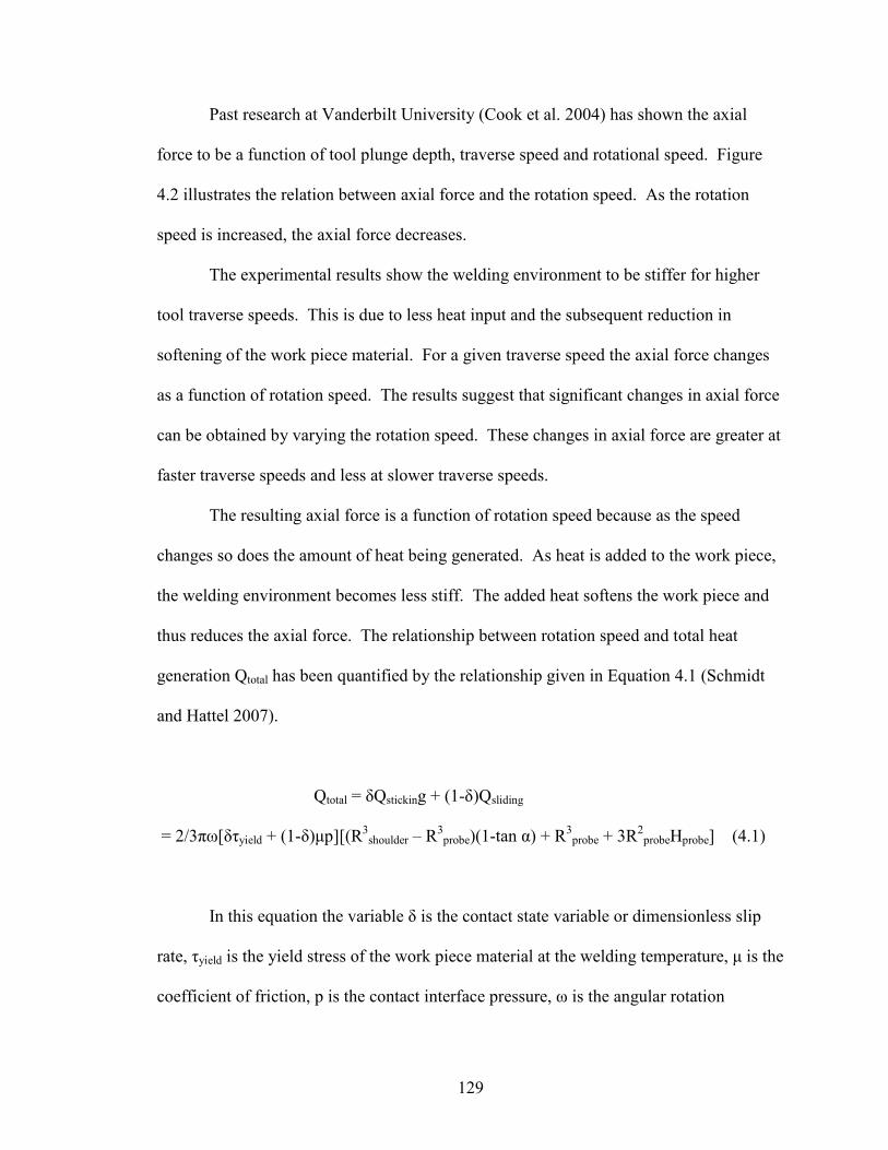
129

Past research at Vanderbilt University (Cook et al. 2004) has shown the axial

force to be a function of tool plunge depth, traverse speed and rotational speed. Figure

4.2 illustrates the relation between axial force and the rotation speed. As the rotation

speed is increased, the axial force decreases.

The experimental results show the welding environment to be stiffer for higher

tool traverse speeds. This is due to less heat input and the subsequent reduction in

softening of the work piece material. For a given traverse speed the axial force changes

as a function of rotation speed. The results suggest that significant changes in axial force

can be obtained by varying the rotation speed. These changes in axial force are greater at

faster traverse speeds and less at slower traverse speeds.

The resulting axial force is a function of rotation speed because as the speed

changes so does the amount of heat being generated. As heat is added to the work piece,

the welding environment becomes less stiff. The added heat softens the work piece and

thus reduces the axial force. The relationship between rotation speed and total heat

generation Qtotal has been quantified by the relationship given in Equation 4.1 (Schmidt

and Hattel 2007).

Qtotal = δQsticking + (1-δ)Qsliding

= 2/3πω[δτyield + (1-δ)µp][(R3shoulder – R

3probe)(1-tan α) + R

3probe + 3R

2probeHprobe] (4.1)

In this equation the variable δ is the contact state variable or dimensionless slip

rate, τyield is the yield stress of the work piece material at the welding temperature, µ is the

coefficient of friction, p is the contact interface pressure, ω is the angular rotation

130

velocity, α is the cone angle of the tool’s pin, Rshoulder is the shoulder radius of the tool,

Rprobe is the radius of the tool’s pin, and lastly, Hprobe is the height of the tool’s pin.

Schmidt and Hattel go on to note the typical expression for a numerical model is in the

form of a position dependent surface flux qtotal. The units of the model would take the

form of power per unit area. In its final form the heat generation model can be expressed

as Equation 4.2, which is a radius dependant surface flux. The simplified equation

assumes tool geometry of only a flat shoulder.

qtotal = (3Qtotalr) / (2πR3shoulder) (4.2)

Historically, force control of FSW has been accomplished by varying the plunge

depth of the tool. Examples are found in the published work by Smith (2000), Soron and

Kalaykov (2006) and Zhao et al. (2007). Each of these groups developed and

implemented a force control architecture using plunge depth as the controlling variable.

All were able to conclude it was feasible to implement FSW force control. However,

using plunge depth as the controlling variable presents several challenges. Soron and

Kalaykov concluded that even with the implemented action of force control to a robotic

FSW system, axial force oscillations will exist when the tool makes contact with the

material. They also note the penetration depth is hard to predict due to the positioning

error of the robot. Zhao et al. presented a non-linear axial force controller they developed

and implemented for a FSW process. They were able to experimentally characterize the

static and dynamic behavior of the interaction between the FSW tool and the work piece.

With this information and using an open architecture control system they were able to

131

design a controller using Polynomial Pole Placement. Good results were obtained, but to

handle the non-linear transient response when the tool’s plunge depth changed, the

control system had to incorporate experimentally obtained dynamic parameters. Thus the

open architecture of the control platform was needed in order to implement this force

controller and the controller parameters were specific to their experimental setup.

Axial force is a function of plunge depth, traverse rate and rotation rate. Since it

is challenging to control axial force via plunge depth, this presented research investigates

the use of rotation speed as the controlling variable. The goal of this research was to

investigate, identify and characterize distinguishing features of force control using

rotation speed as the controlling variable. To accomplish this goal, a FSW force

controller that utilized tool rotation speed as the controlling variable was created and its

performance analyzed.

If it is desired to control axial force while welding on a flat uniform surface, using

plunge depth as the controlling variable might not be necessary? Results from this

presented research shows axial force can be controlled via rotation speed. It is concluded

that the controller manages the generation of heat so as to create both uniform thermal

and uniform force conditions along the weld seam.

Experimental Setup

The experiment was conducted on the FSW system at Vanderbilt University

which is shown in Figure 4.3. The FSW system is a Milwaukee Model K milling

machine that has been retrofitted with more advanced motors and instrumentation. These

retrofits were previously added to automate the system and provide a programmable

132

platform for FSW experimentation. At the top of the control hierarchy is a master

computer that enables all of the systems subcomponents such as the motor drive

controllers and instrumentation. The master computer is a Dell Precision 340 that uses

Microsoft Windows XP as its operating system. The welding and force control code was

written in C#. A graphical user interface within the C# software allows the operator to

select the desired welding parameters for the pending operation. These parameters

include the FSW tool’s rotation speed, traverse speed, plunge depth and path position.

A 20 horsepower, Baldor Industrial VM251T motor is used to drive the spindle

through an attached pulley and belt system. The spindle motor is controlled by a Cutler-

Hammer SVX9000 Sensorless Vector variable frequency drive (VFD). Command

signals are sent directly from the master computer to the VFD. With this system the

machine is capable of spindle speeds from 100 revolutions per minute (RPM) to 2000

RPM.

Figure 4.3: FSW machine at Vanderbilt University (Sinclair 2009).

133

Welding force data is collected through a Kistler Rotating Cutting Force

Dynamometer. The dynamometer collects x-axis force, y-axis force, z-axis force as well

as the torque about the z axis. The analog signal from the dynamometer is sent to a signal

conditioning box were it is converted from an analog signal to a digital signal. Once

converted the data is sent to a separate computer where the data is sorted, recorded and

displayed before being sent to the master computer.

Figure 4.4: Block diagram of force control via rotation speed.

An overview of the closed loop force control system is illustrated by the control

block diagram of Figure 4.4. Within the master computer a desired z force is selected.

The desired force value is subtracted from the actual z force value to obtain a force error.

The force error signal is then processed in the control law. The resulting processed

control signal is then multiplied by a factor of 0.15 to translate the signal from Newtons

of force to desired revolutions per minute of rotation speed. The desired RPM is

converted to the corresponding frequency and then sent to the VFD. The VFD produces

the desired change in rotation speed to obtain the desired value of z force in the welding

134

environment. The dynamometer reads the resulting force and returns it to the master

computer where it is once again compared to the reference signal.

The measured z force signal was very noisy. This noise makes the process of

applying derivative control to the system very difficult. The noise would simply be

amplified by the controller. To address this problem, a filter was implemented. The filter

is a five point moving average of the z force with an interrupt frequency of 3.33 Hz. For

this experimental setup these filter parameters were found to provide adequate noise

reduction without adding too much phase lag in the signal.

The control law consisted of proportional, integral plus derivative (PID) control.

Due to the retrofitted nature of the FSW system there are several unknown parameters

that could not be accurately modeled to create a non-linear modeled based control

system. For instance, the force control loop resides outside the control loop for the

spindle drive. The Cutler-Hammer VFD uses its own proprietary control techniques to

drive the motor. Thus, obtaining the parameters of the VFD as well the physical

parameters of the spindle motor would require an extensive amount of testing and

analysis. In addition, the time needed for signal processing and transmission through the

master computer, dynamometer, sensor box and the VFD would also have to be

experimentally determined. With all of these variables to consider the potential

performance of a model based controller might not be much better than a standard PID

controller. For this experimentation to create and investigate the performance of z axis

force control via rotation speed, PID control architecture was chosen as the best option.

To address the transport delay between the initiation of the control signal and the

change in force, a simple delay of 1 second in the control update time was utilized. The 1

135

second delay allowed the FSW tool to change speed and a change in z force to occur.

The delay in the control signal update proved to be effective without the need of adding a

more complicated controls approach such as a Smith Predictor-Corrector.

To tune the PID force controller and achieve optimum control, the Ziegler-

Nichols tuning process was used (Ogata 2002). The Ziegler-Nichols tuning process

called for the controller to use only proportional gain while welding. While using

proportion control only, a critical gain value was experimentally determined through trial

and error. Over the course of several welds, the gain was steadily increased until the

resulting z force achieved sustained oscillation. The sustained oscillation constituted

marginally stable behavior. The resulting control gain and time period between

oscillations was recorded and used to calculate PID gains for the controller. The

resulting PID control law is shown in Equation 4.3. In Equation 4.3, Kp is the

proportional gain, Ki is the integral gain, Kd is the derivative gain, e is the error and u is

the resulting control signal as a function of time t.

Kp e + Ki ∫e + Kd e΄ = u(t) (4.3)

The FSW tool consisted of a slightly undersized 1/4 inch Trivex pin with a flat

5/8 inch diameter shoulder. The Trivex profile geometry is similar to an equilateral

triangle but with its edge surfaces slightly convex. The pin with its Trivex geometry was

0.235 inches long by 0.210 inches across its widest point. Using the Ziegler-Nichols

tuning method, a critical gain was determined for the tool. The critical gain and period

136

for the ¼ inch Trivex tool was 2.9 and 13.0 seconds respectively. The resulting control

gains are shown in Table 4.1.

For the experiment, ¼ inch butt welding with full penetration was performed.

The material used was aluminum 6061. The work piece consisted of two ¼ inch by 1 ½

inch by 8 inch long samples. Each weld began with the tool plunging into the metal 1

inch from the end of the work piece. Once the tool achieved the desired plunge depth it

dwelled at that location for 5 seconds in order to soften the work piece by generating

additional heat. After dwelling, the tool began to traverse forward at 6 inches per minute

(IPM). After traversing 1 inch the force controller was engaged. The force controller

operated in a regulation mode, meaning that whatever the z force was at the time of

engagement, it was the selected desired force. The system operated under force control

mode until it reached 1 inch from the end of the 8 inch work piece. Thus 5 inches of

welding was conducted for each run under force control. For many of the welds a step

input in desired force occurred after 2 inches of regulation. Each step input was 500

Newtons in magnitude. For every weld made, the tool’s shoulder was plunged 0.001 –

0.005 inches below the surface and the tool’s traverse rate was maintained at a constant 6

IPM. Prior to engaging the force control the rotation speed was 1100 - 1200 RPM.

Table 4.1: Rotation Mode Force Control Gains.

137

100 120 140 160 180 200 220 240 260 280 3000

1000

2000

3000

4000

5000

6000

7000

8000Z-Force (Newtons) as a Function of Time (seconds)

Z-Force (N)

Time (sec)

Actual Z Force

Desired Z Force

Pin Plunge

Shoulder Plunge

Weld

Force

Control

Start/Stop

Zone

Traverse Forward

Figure 4.5: Weld sample with no force control.

To provide a base line of the welding environment, a weld was made without any

force control using the ¼ inch Trivex tool. The results are shown in Figure 4.5. The

resulting force during the initial tool plunge into the work piece is identified on the figure

as the pin plunge and shoulder plunge regions. After the tool has plunged into the work

piece and dwelled for 5 seconds, the forward motion of the tool begins. This point is

easily identified as the sharp increase in force after the shoulder plunge and dwell period.

After 1 inch of forward travel the force controller is normally engaged at this point.

However, for this base line sample the force controller is not engaged, but the force

occurring at the engagement point is displayed as a desired force reference. From the

base line sample it can clearly be seen that the z force continues to increase about two

138

thirds of the distance across the weld seam. The increase is due to the tool moving into

un-welded and colder material. This also indicates the welding process has not yet

reached a steady state.

Past the two thirds point the z force briefly maintains a steady value before

beginning to drop in value. This drop in z force is due to the heat build up on the end of

the 8 inch weld sample. At the end of the sample the heat conduction has to rely largely

on convection to transfer heat out of the work piece. The rate of conduction is much

faster than the rate of convection for this particular configuration. Thus the heat tends to

build up on the end of the work piece. As the tool continues to traverse toward the end of

the work piece, it moves into the hotter and softer region thus lowering the z force.

It can be concluded that the welding process never truly reaches a steady state

condition for this particular setup. These transient conditions will provide a good

environment to observe the response of the force controller. The system will encounter

disturbances that will produce an ever changing error signal for the controller to process

and respond to.

Results and Discussion

Successful control of axial force was obtained by the aforementioned

experimental setup. The controller was able to regulate to a desired force reasonably

well. However relatively large changes in force were found to be difficult due to the

limits in spindle RPM. Changes in force greater than 700 Newtons were not obtainable

simply because the milling machine could not obtain speeds outside of the range of 800 –

2000 RPM. For the controller to maintain a desired force, it required significant tool

139

speed adjustments from the milling machine. The changing speed is evident by the

surface texture of the weld seam shown in Figure 4.6.

Another interesting aspect of force control via rotation speed discovered was the

slow and unpredictable response times. From a qualitative standpoint the force controller

can be described as sluggish in its response. One resolution for this sluggish behavior

was found. Improved response time was obtained by using greater plunge depths.

Plunge depths that established 100% shoulder contact with the work piece surface created

better force responses. However the drawback to the increased plunge depth was weld

flash.

Figure 4.6: Welded sample using force control via rotation speed.

Figure 4.7 shows the axial force response under force control. The force was

regulated to a desired value of 6505 Newtons. Notice the relatively large range of RPM

adjustments needed to maintain the desired force. For the 5 inches of welding, the

controller adjusted the rotation speed over a range of approximately 700 RPM. The short

span of welding utilized 58% of the spindle adjustment capacity of the machine, based

140

upon a 1200 RPM range. If the weld seam was several dozen inches long, a machine

with a much larger range of spindle speeds would be needed.

Most of the spindle adjustment was needed during the first half of the welding

operation. Referring to the baseline weld of Figure 4.5, this is the region where there is

naturally an increase in force due to the changing thermal conditions underneath the tool

as it begins to move into a colder region. The changing thermal condition is countered by

the tool generating more heat with an increase in RPM. Unlike other force control

strategies where the plunge depth is adjusted to physically cause a change in force; this

controller induces thermal changes to the welding environment.

Along with the slow response time was the lack of a sudden spike in axial force.

A sudden spike is a challenging phenomenon to force control systems. This type of

transient response is seen when the plunge depth is changed and can be a problem for

force control of FSW while using plunge depth as the controlling variable. As evident

from Figure 4.7, that is not the case when tool rotation speed is used as the controlling

variable.

Statistical analysis of the results in Figure 4.7 show the controller was able to

achieve a mean force of 6488 Newtons as compared to a desired force of 6505 Newtons.

The median value was 6490 Newtons while the standard deviation was determined to be

132 Newtons. The maximum value was 6737 Newtons and the minimum value was 6215

Newtons which produced a range of 522 Newtons.

141

230 240 250 260 270 280 290 300

5000

6000

7000

Z-Force (Newtons) as a Function of Time (seconds)

P I D Control 1/4" Trivex

Z-Force (N)

Time (sec)

230 240 250 260 270 280 290 3001000

1200

1400

1600

1800

Tool Rotation Speed (RPM) as a Function of Time (seconds)Tool Speed (RPM)

Time (sec)

Actual Force

Desired Force

Figure 4.7: Regulation of z force via tool rotation speed.

As a comparison to force control of FSW via plunge depth adjustment, standard

deviation values of 130 Newtons have been obtained using the same FSW system at

Vanderbilt University. These results are also similar to results reported by Soron and

Kalaykov (2006). With plunge depth as the controlling variable they were able to regulate

to a desired z force with a standard deviation of 152 Newtons. However they were using

an articulated arm robot and not a milling machine.

Further results from the experimentation can be seen in Figure 4.8 through Figure

4.10. In each of these cases, a step input of 500 Newtons was executed. The results once

again show the controller utilized a large amount of the RPM capacity of the machine.

More apparent though is the lagging response of the system to the step input. This is

especially evident in Figure 4.8 where the system continually lowers the tool’s RPM

value for 3 – 5 seconds without any force response to the step input. A lag in response is

142

also evident in the force oscillations, although some of the oscillations can be attributed

to the integrator in the control algorithm.

230 240 250 260 270 280 290 3005000

6000

7000

8000

Z-Force (Newtons) as a Function of Time (seconds)

P I D Control 1/4" Trivex

Z-Force (N)

Time (sec)

230 240 250 260 270 280 290 3001000

1200

1400

1600Tool Rotation Speed (RPM) as a Function of Time (seconds)

Tool Speed (RPM)

Time (sec)

Actual Force

Desired Force

Figure 4.8: PID Control with a 500N step input, example 1.

230 240 250 260 270 280 290 3005000

6000

7000

8000

Z-Force (Newtons) as a Function of Time (seconds)

P I D Control 1/4" Trivex

Z-Force (N)

Time (sec)

230 240 250 260 270 280 290 300800

1000

1200

1400

1600

1800Tool Rotation Speed (RPM) as a Function of Time (seconds)

Tool Speed (RPM)

Time (sec)

Figure 4.9: PID control with a 500 N step input, example 2.

143

230 240 250 260 270 280 290 3005000

6000

7000

8000

Z-Force (Newtons) as a Function of Time (seconds)

P I D Control 1/4" Trivex

Z-Force (N)

Time (sec)

230 240 250 260 270 280 290 3001000

1200

1400

1600

1800Tool Rotation Speed (RPM) as a Function of Time (seconds)

Tool Speed (RPM)

Time (sec)

Actual Force

Desired Force

Figure 4.10: PID control with a 500 N step input, example 3.

This lag response in force control via rotation speed adjustment is probably due to

the complex thermal condition of the welding environment? A possible explanation for

the lag is the amount of time need for the heat to be generated and then transferred? As

heat is generated within the welding environment it diffuses outward to the surrounding

environment. The entire process of heat generation and transfer in FSW is not well

understood but fundamentally it is known that hotter welding conditions are associated

with a lower axial force. In addition, heat build up in the welding environment depends

on the thermal conductivity in the surrounding area of the welding process. This includes

the work piece geometry, backing anvil, clamps and the tool. Combined together these

items create a very complex situation determining heat transfer in the localized welding

environment. The lag in the force response to the changing tool speed might also be due

to the time need for heat to build up in the localized welding area? If the surrounding

environment is favorable to heat transfer, then the response time could be prolonged. In

144

contrast if the surrounding area is not favorable to heat transfer, the response time could

be quicker. Thus although the force is controlled by the amount of heat being generated,

the thermal conductivity of the localized welding environment plays a role in the

response time.

To verify the quality of the produced welds, macro cross sections were produced.

The primary reason for inspecting these cross sections was too see if changing rotation

speed during the welding cycle produced welding flaws such as internal voids. Upon

review of the cross sections shown in Figure 4.11 and Figure 4.12, no internal voids were

found. The cross sections were taken of weld samples where step inputs occurred, such

as the ones shown in Figures 4.8 through Figure 4.10. The cross sections revel a rather

large area of refined grain size. This refined grain indicates the area was subjected to

severe plastic deformation and consolidation of the parent metals occurred.

Another feature noticeable in the cross sections is the weld flash at the work

piece’s surface. This flash is rather large and undesirable in most situations. This flash

was a result of the large plunge depths needed in order to obtain reasonable response

times from the controller.

Figure 4.11: Cross section of a weld seam, example 1.

145

Figure 4.12: Cross section of a weld seam, example 2.

Conclusions

Force control via tool rotation speed is a viable process. The results show that the

performance level of control is comparable to other systems that use plunge depth as the

controlling variable. However it can not be applied in all situations. A few conditions

have to be present before this becomes a viable method for controlling force.

First, it must be acceptable for the plunge depth to remain constant. Previous

FSW force control systems utilized plunge depth as the controlling variable to adjust to

changing conditions in the work piece or with the applying machinery. Typically the

machine was a robot. With tool rotation speed as the controlling variable, adaptations to

physical changes in the work piece or deflection in the machine components (robots) can

not be achieved. If constant plunge depth can be maintained, using the tool’s rotation

speed as the controlling variable is an attractive alternative. It is attractive because it is

much easier to control than plunge depth. One of the challenges of using plunge depth as

the controlling variable is the resulting transient force when the plunge depth is changed.

This transient force can create stability issues for the controller. However with rotation

speed as the controlling variable, the ill behaved transient force is not present.

Second, it must be acceptable to have weld flash present. Force control was not

realized unless the entire shoulder was submerged into the work piece. With the entire

146

shoulder being in contact with the work piece, no significant change in force occurred

over the range of available rotation speeds. However, flash can be minimized by using

tools with features on their shoulders that allow for a 0° lead angle. Features such as

scrolls will enhance the metal flow, reduce flash and produce acceptable welds at a 0°

lead angle.

Future research can be performed with force control via rotation speed while a

scrolled shoulder tool is positioned at a 0° lead angle. In addition, the force control

architecture should be implemented on a machine with a larger range of available spindle

speeds.

147

CHAPTER V

AN INVESTIGATION OF FORCE CONTROLLED FRICTION STIR WELDING FOR MANUFACTURING AND AUTOMATION

William R. Longhurst, Alvin M. Strauss, George E. Cook, Chase D. Cox,

Christopher E. Hendricks, Brian T. Gibson, Yannick S. Dawant

Proceedings of the Institution of Mechanical Engineers, Part B, Journal of Engineering

Manufacture. Status: Submitted June 30, 2009, revised October 4, 2009 and accepted for

publication October 20, 2009.

Abstract

Friction Stir Welding (FSW) is a solid state joining process for materials with low

melting points. The process uses a rotating tool that consists of a shoulder and a pin. The

tool plastically deforms the material with its pin and then forges together the parent

materials underneath the shoulder. Past research has established that the axial force on

the tool that creates the forging pressure is a function of plunge depth, traverse speed and

rotation speed. Historically, force control of FSW has been accomplished by varying the

plunge depth of the tool.

The research present in this paper examines force control of FSW via varying

each of the process parameters separately. A force controller was implemented on a

retrofitted milling machine. The closed loop proportional, integral plus derivative (PID)

control architecture was tuned using the Ziegler-Nichols method. Welding experiments

148

were conducted by butt welding ¼ inch (6.35 mm) x 1 ½ inch (38.1 mm) x 8 inch (203.2

mm) samples of aluminum 6061-T6511 with a ¼ inch (6.35 mm) FSW tool.

The results indicate that force control via traverse speed is the most accurate and

as a byproduct heat distribution control along the weld seam occurs. Force control via

plunge depth is the least accurate but it compensates for machine and robot deflection.

Tensile test data shows that greater strength can be obtained through force control via

rotation speed.

It is concluded that force is maintained by keeping the amount of tool surface area

in contract with the work piece constant throughout the welding process when plunge

depth is used as the controlling variable. Force is maintained by varying the rate of heat

generation when rotation speed is used as the controlling variable. Lastly force is

maintained by changing the amount of heat deposited per unit length along the weld seam

when traverse speed is used as the controlling variable. Successful robotic FSW requires

selecting the appropriate controlling variable and reducing the sensitivity of the

interaction between the tool and the work piece.

Introduction

Friction Stir Welding (FSW) is relatively new method of joining materials. The

process was invented by Wayne Thomas of The Welding Institute (TWI) and patented in

1995 (Thomas et al. 1995). It is a solid state welding process that offers many

advantages over fusion welding processes. It is used to join metals with low melting

points such as aluminum. The FSW process utilizes a rotating non-consumable tool to

149

perform the welding process. In its simplest form the rotating tool consists of a small pin

(or probe) underneath a larger shoulder. The FSW process is illustrated in Fig. 5.1.

This welding process uses thermo-mechanical mechanisms to join the parent

metals of the work piece. These mechanisms include heat generation, plastic deformation

and forging. Heat is generated from both friction and plastic deformation. The heat

softens the work piece which lowers the forces needed for further plastic deformation and

forging. As the tool rotates and travels through the work piece along the faying surface,

it plastically deforms the parent metals that define the work piece. As the pin rotates

within the work piece it shears a thin layer of the material. The deformed material is

rotated around to the pin’s backside where it is consolidated under the forging pressure

from the shoulder. Forging pressure is created by firmly holding the tool in the work

piece with a sufficient axial force. The plastic deformation and ensuing forging action,

bonds the parent materials together.

Figure 5.1: Illustration of the FSW process.

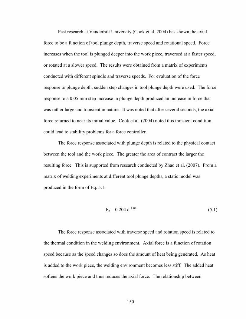
150

Past research at Vanderbilt University (Cook et al. 2004) has shown the axial

force to be a function of tool plunge depth, traverse speed and rotational speed. Force

increases when the tool is plunged deeper into the work piece, traversed at a faster speed,

or rotated at a slower speed. The results were obtained from a matrix of experiments

conducted with different spindle and traverse speeds. For evaluation of the force

response to plunge depth, sudden step changes in tool plunge depth were used. The force

response to a 0.05 mm step increase in plunge depth produced an increase in force that

was rather large and transient in nature. It was noted that after several seconds, the axial

force returned to near its initial value. Cook et al. (2004) noted this transient condition

could lead to stability problems for a force controller.

The force response associated with plunge depth is related to the physical contact

between the tool and the work piece. The greater the area of contract the larger the

resulting force. This is supported from research conducted by Zhao et al. (2007). From a

matrix of welding experiments at different tool plunge depths, a static model was

produced in the form of Eq. 5.1.

Fz = 0.204 d 1.84 (5.1)

The force response associated with traverse speed and rotation speed is related to

the thermal condition in the welding environment. Axial force is a function of rotation

speed because as the speed changes so does the amount of heat being generated. As heat

is added to the work piece, the welding environment becomes less stiff. The added heat

softens the work piece and thus reduces the axial force. The relationship between

151

rotation speed and total heat generation Qtotal has been quantified by the relationship

given in Eq. 5.2 (Schmidt and Hattel 2008).

Qtotal = δQsticking + (1-δ)Qsliding

= 2/3πω[δτyield + (1-δ)µp][(R3shoulder – R

3probe)(1-tan α) + R

3probe + 3R

2probeHprobe] (5.2)

In this equation the variable δ is the contact state variable or dimensionless slip rate, τyield

is the yield stress of the work piece material at the welding temperature, µ is the

coefficient of friction, p is the contact interface pressure, ω is the angular rotation

velocity, α is the cone angle of the tool’s pin, Rshoulder is the shoulder radius of the tool,

Rprobe is the radius of the tool’s pin, and lastly, Hprobe is the height of the tool’s pin.

Axial force is a function of traverse speed because the stiffness of the welding

environment beneath the tool changes as the speed changes. A faster moving tool will

not deposit as much heat in a localized region. The colder welding condition results in a

greater axial force. The opposite occurs when the tool is traveling at a slower rate.

Force control is used for robotic applications of FSW. Cook et al. (2003) stated

force control is key to providing control of FSW with industrial robots. Force control is

needed to compensate for the deflection of the robot linkages when subjected to the rather

large forces associated with FSW and to adjust to physical variations in the work piece

surface. Robots can not compensate for linkage deflection while under pure position

control. Robots use feedback from motor encoders to calculate the position of each of

their linkages. Encoders detect the position of the motor shaft that positions the linkage.

They cannot sense any deflection that occurs in the linkage itself. The robot’s central

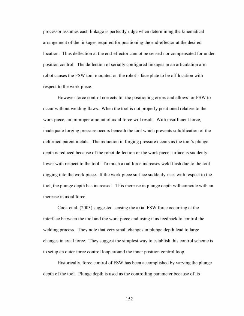
152

processor assumes each linkage is perfectly ridge when determining the kinematical

arrangement of the linkages required for positioning the end-effector at the desired

location. Thus deflection at the end-effector cannot be sensed nor compensated for under

position control. The deflection of serially configured linkages in an articulation arm

robot causes the FSW tool mounted on the robot’s face plate to be off location with

respect to the work piece.

However force control corrects for the positioning errors and allows for FSW to

occur without welding flaws. When the tool is not properly positioned relative to the

work piece, an improper amount of axial force will result. With insufficient force,

inadequate forging pressure occurs beneath the tool which prevents solidification of the

deformed parent metals. The reduction in forging pressure occurs as the tool’s plunge

depth is reduced because of the robot deflection or the work piece surface is suddenly

lower with respect to the tool. To much axial force increases weld flash due to the tool

digging into the work piece. If the work piece surface suddenly rises with respect to the

tool, the plunge depth has increased. This increase in plunge depth will coincide with an

increase in axial force.

Cook et al. (2003) suggested sensing the axial FSW force occurring at the

interface between the tool and the work piece and using it as feedback to control the

welding process. They note that very small changes in plunge depth lead to large

changes in axial force. They suggest the simplest way to establish this control scheme is

to setup an outer force control loop around the inner position control loop.

Historically, force control of FSW has been accomplished by varying the plunge

depth of the tool. Plunge depth is used as the controlling parameter because of its

153

relationship to the physical interaction between the tool and the work piece. While under

force control, work piece surface variation and deflection in robot linkages do not cause

welding flaws if plunge depth is used as the control variable. If surface variation and

robot linkage deflection occurs without force control, the FSW tool would either plunge

deeper into the work piece or withdraw. In either case the welding force would change

dramatically. In force control architectures similar to the one suggested by Cook et al.

(2003), the force controller is the master controller while the position controllers for the

robot’s linkages are slaved to the force controller. Thus the force controller will vary the

position of the linkages to maintain a desired force in the FSW environment. A force

control strategy is also more desirable since acceptable welding can occur over a relative

wide range of forces but it cannot occur over a wide range of plunge depths (Smith

2007).

Examples of robotic FSW that use force control are found in the published work

by Smith (2000), Soron and Kalaykov (2006), and Zhao et al. (2008). Each of these

groups developed and implemented a force control architecture using plunge depth as the

controlling variable. Their research was focused primarily on robotic integration. All

were able to conclude it was feasible to implement force control for robotic FSW.

However, using plunge depth as the controlling variable presents several challenges.

Smith (2000) reported the ability to use actuator torques as a measurement of the

FSW force through the Jacobian relationship (Craig 2005). The process was limited by

the computation time needed. The controller was able to produce an updated control

signal up to 2 Hz. Smith used an ABB IRB 6400 robot with its open architecture to

implement force control. He concluded that the update time is not adequate for force

154

control during the plunging operation and that deflections in the traverse direction must

be overcome with programming offsets.

Soron and Kalaykov (2006) used an ABB IRB-7600-500 serial robot for their

experimentation. They replace the sixth axis with FSW tooling including an ATI Omega-

190 force and torque sensor. Two types of robot controllers are used. The first was the

ABB S4C + which has force control based on an existing path corrector option in the

program. The second controller was the ABB IRC5 which uses force control for standard

industrial operations such as grinding and assembly. The pre-existing software package

for these operations has the force control embedded. They adapted grinding and

assembly instructions to FSW to utilize the commercially developed software for force

control of FSW. They conclude it is feasible to implement force control. However they

noted a few drawbacks such as force oscillations, predicting penetration depth and

defining the welding trajectory in 3-dimensions with high precession.

Zhao et al. (2008) developed a controller from experimental data obtained while

welding using an ABB IRB 940 Tricept robot. With their experimental data they were

able to create static and dynamic models of the welding system. With these models, they

used a Polynomial Pole Placement method to design the controller. The controller was

then implemented in a Smith Predictor – Corrector structure to compensate for the system

delays (Ogata 2002). Their controller was able to maintain a constant axial force as the

tool crossed gaps in the work piece.

Axial force is coupled to the parameters of plunge depth, traverse rate and rotation

rate in a highly nonlinear manner. This coupled nonlinear relationship makes the

implementation of force control over a wide range of parameters extremely difficult.

155

Since it is challenging to control axial force, this presented research investigates and

compares the controlling effect of each of the process parameters. The goal of this

research was to investigate, identify and characterize the contributing features of force

control from each of the controlling variables. To accomplish this goal, a FSW force

controller that utilized each of the parameters separately as the controlling variable was

created and its performance analyzed.

Results from this presented research shows axial force can be controlled via

plunge depth, traverse speed or rotation speed. It is concluded that the controller

manages the generation of heat so as to create both uniform thermal and uniform force

conditions along the weld seam when rotation speed is used as the controlling variable.

When traverse speed is used, the control of weld seam heat distribution is obtained as a

by product of force control. When the plunge depth is used, the physical interaction

between the tool and the work piece remains constant due to force control.

Experimental Setup

The experiment was conducted on the FSW system at Vanderbilt University

which is shown in Fig. 5.2. The FSW system is a Milwaukee Model K milling machine

that has been retrofitted with more advanced motors and instrumentation. At the top of

the control hierarchy is a master computer that enables all of the systems subcomponents

such as the motor drive controllers and instrumentation.

The tool’s vertical axis coincides with the milling machine worktable’s vertical

axis when the tool is at a zero degree tilt angle. The worktable resides on the knee that is

mounted to a vertical positioning screw and secured in sliding dovetail joints. The knee

156

travels on the screw via a gear system inside the knee. An externally mounted belt and

pulley system is attached to the input shaft of the gear system. Power is provided by a

Parker Compumoter KH series brushless servo motor. The servo motor is controlled by a

Parker Compumotor KHX-250 servo drive. Command signals are sent directly from the

master computer to the servo drive. Vertical position of the table is obtained from a

Reinshaw linear scale that has a resolution of 10 micrometers (0.0004 inches).

Figure 5.2: FSW machine at Vanderbilt University.

The traverse axis coincides with the milling machine worktable’s cross axis. The

worktable resides in its saddle by sliding dovetail joints and is driven by a power screw.

The power screw is rotated via a system that consists of a belt and pulley attached to the

shaft of the power screw. A 1 horsepower (745.70 Watts), 6.02 reduction Syncrogear

gear motor is attached to the drive pulley. The gear motor is controlled by a Cutler-

Hammer MVX9000 Sensorless Vector variable frequency drive (VFD). Command

157

signals are sent directly from the master computer to the VFD. Traverse position is

obtained from a string potentiometer.

A 20 horsepower (14914 Watts), Baldor Industrial VM251T motor is used to

drive the spindle through an attached pulley and belt system. The spindle motor is

controlled by a Cutler-Hammer SVX9000 Sensorless Vector variable frequency drive

(VFD). Command signals are sent directly from the master computer to the VFD.

Welding force data is collected through a Kistler Rotating Cutting Force

Dynamometer. The dynamometer collects x-axis force, y-axis force, z-axis force as well

as the torque about the z-axis. Before computing the force error the force signal is

filtered using a five point moving average with an interrupt frequency of 3.33 Hz.

Figure 5.3: Block diagram of force control.

An overview of the closed loop force control system is illustrated by the control

block diagram of Fig. 5.3. The force control loop resides outside of the control loop for

the selected machine axis. The resulting processed control signal from the force

controller is used to alter the selected controlling variable of plunge depth, traverse speed

158

or rotation speed from its reference value. The axis reference signal is the initial plunge

depth, traverse speed or rotation speed at the time of engagement of force control. The

selected machine axis and its controller produce the desired change in plunge depth,

traverse speed or rotation speed to obtain the desired value of z force in the welding

environment. The dynamometer reads the resulting force and returns it to the force

controller where it is compared to the reference signal.

The control law consisted of proportional, integral plus derivative (PID) control.

To tune the PID force controller and achieve optimum control, the Ziegler-Nichols tuning

process was used (Ogata 2002). The Ziegler-Nichols tuning method is used for tuning

systems of unknown dynamics. For a closed looped system under proportional gain only,

the gain is steadily increased until an oscillation of the output force is sustained. The

critical gain that produces sustained oscillation represents the point of marginal stability

for the system. If the system could be analyzed using the root-locus method, the point of

marginal stability would be the point where the locus crossed the vertical axis in route

from the left hand plane into the right half plane. By using the established critical gain

and the measured period of oscillation, stable gains for a PID controller can be calculated

using predetermined formulas. The resulting PID control law is shown in Eq. 5.3. In Eq.

5.3, Kp is the proportional gain, Ki is the integral gain, Kd is the derivative gain, e is the

error and u is the resulting control signal as a function of time t. The calculated gains

from the Ziegler-Nichols tuning process are listed in Table 5.1.

Kp e(t) + Ki ∫e(t) + Kd e΄(t) = u(t) (5.3)

159

For the experiment, ¼ inch (6.35 mm) butt welding with full penetration was

performed. The material used was aluminum 6061-T6511. The work piece consisted of

two ¼ inch (6.35 mm) by 1 ½ inch (38.1 mm) by 8 inch (203.2 mm) long samples. Each

weld began with the tool plunging into the metal 1 inch (25.4 mm) from the end of the

work piece. Once the tool achieved the desired plunge depth it dwelled at that location

for 5 seconds in order to soften the work piece by generating additional heat. After

dwelling, the tool began to traverse forward. After traversing 1 inch (25.4 mm) the force

controller was engaged. The force controller operated in a regulation mode, meaning that

whatever the z force was at the time of engagement, it was the selected desired force.

The system operated under force control mode until it reached 1 inch (25.4 mm) from the

end of the 8 inch (203.2 mm) work piece. Thus 5 inches (127.0 mm) of welding was

conducted for each run under force control.

Table 5.1: Control gains.

160

The tools used for the welding were a ¼ inch (6.35 mm) Trivex tool and a ¼ inch

(6.35 mm) thread tool. The tools are shown in Fig. 5.4. For force control via traverse

speed and rotation speed the Trivex tool was used. For force control via plunge depth,

the threaded tool was used with its tapered shoulder.

Figure 5.4: Trivex and threaded FSW tools.

100 120 140 160 180 200 220 240 260 280 3000

1000

2000

3000

4000

5000

6000

7000

8000Z-Force (Newtons) as a Function of Time (seconds)

Z-Force (N)

Time (sec)

Actual Z Force

Desired Z Force

Pin Plunge

Shoulder Plunge

Weld

Force

Control

Start/Stop

Zone

Traverse Forward

Figure 5.5: Weld sample with no force control.

161

To provide a base line of the welding environment, a weld was made without any

force control. The results are shown in Fig. 5.5. The resulting force during the initial

tool plunge into the work piece is identified on the figure as the pin plunge and shoulder

plunge regions. After the tool has plunged into the work piece and dwelled for 5 seconds,

the forward motion of the tool begins. The z force continues to increase as the tool

traverses across the weld seam. The increase is due to the tool moving into un-welded

and colder material.

Near the end of the weld the z force begins to drop in value. This drop in z force

is due to the heat build up on the end of the weld sample. As the tool continues to

traverse toward the end of the work piece, it moves into the hotter and softer region thus

lowering the z force.

A small portion of the increase in force can be attributed to thermal expansion of

the tool and the work piece. Temperature measurements indicate the tool reaches a

maximum temperature of approximately 90° C at a point 1.5 inches (38.1 mm) above the

shoulder. However by the end of the initial plunge the tool has reached 50 % of its

maximum temperature. Thus a temperature change (∆T) of 34° C occurs during the

forward movement of the tool. As shown in Eq. 5.4, this equates to a maximum

expansion (∆L) of .0019 inches (0.048 mm) for a 4 inch (101.6 mm) long tool (L) made

of H13 tool steel (expansion coefficient α = 13.1 x 10-6).

This estimate is an upper bound because it assumes that one end of the tool is

constrained from expansion. In reality it is only constrained at its edges. When the ¼

inch (6.35 mm) thick aluminum work piece reaches the same temperature, the maximum

thermal expansion is 0.0005 inches (0.0127 mm) (expansion coefficient for aluminum α =

162

13.1 x 10-6). Once again this is an upper bound since the work piece is clamped along its

top surface.

∆L = α x ∆T x L (5.4)

Results and Discussion

Force Response

Without force control via plunge depth, welding flaws can develop when the

surface conditions of the work piece change or when robot and machine linkages deflect

under loading conditions. These welding flaws included weld flash and reduced load

bearing capability. An example is shown in Fig 5.6. Figure 5.6 shows the results of no

force control when one end of the work piece is elevated 1 mm (0.039 inches) above the

other. Figure 5.7 shows the corresponding force and position data during this weld.

As can clearly be seen the tool did not adjust to the changing elevation of the

work piece. The tool simply continued forward and dug into the work piece causing a

significant amount of weld flash.

Figure 5.6: Welding without force control.

163

220 240 260 280 300 320 3400

5000

10000Z-Force (Newtons) as a Function of Time (seconds) -No Force Control.

Z-Force (N)

Time (sec)

220 240 260 280 300 320 3406.2

6.25

6.3

6.35

6.4Verticle Position (inches) as a Function of Time (seconds)

Ver Position (in)

Time (sec)

Figure 5.7: Force and position response with no force control.

In contrast, Fig. 5.8 and Fig. 5.9 shows the result when force control is used to

adjust to the work piece being elevated by 1 mm (0.039 inches) on one end. The force

controller was able to adjust the position of the tool and prevent it from digging into the

work piece.

Figure 5.8: Welding with force control.

164

220 240 260 280 300 320 3405000

6000

7000

8000

9000

10000Z-Force (Newtons) as a Function of Time (seconds)

Z-Force (N)

Time (sec)

220 240 260 280 300 320 3405.6

5.61

5.62

5.63

5.64

Verticle Position (inches) as a Function of Time (seconds)Ver Position (in)

Time (sec)

Actual Force

Desired Force

Actual Position

Reference Position

Figure 5.9: Force and position response under force control.

As another example of force control, Fig. 5.10 and Fig 5.11 show the adjustment

to a 1 mm (0.039 inches) step input. The sudden disturbance caused by the change in

material thickness causes some initial flash but the force controller is able to reposition

the tool and eliminate the flash.

Figure 5.10: Welding with force control over a 1 mm step.

165

240 260 280 300 320 340 3605000

6000

7000

8000Z-Force (Newtons) as a Function of Time (seconds)

Z-Force (N)

Time (sec)

Actual Force

Desired Force

240 260 280 300 320 340 3605.4

5.42

5.44

5.46Verticle Position (inches) as a Function of Time (seconds)

Ver Position (in)

Time (sec)

Actual Position

Reference Position

Figure 5.11: Force and position response to 1 mm step.

Figure 5.12 compares the force response when different controlling variables are

used to regulate the force. Fig. 5.12 a) illustrates the response when traverse speed is

used as the controlling variable. Fig. 5.12 b) illustrates the response when rotation speed

is used as the controlling variable, while Fig. 5.12 c) illustrates the response when plunge

depth is used.

Force control via traverse speed produces the most accurate response with the

least amount of variation. It is the most accurate because the mean force error (mean

force value – desired value) is 0.06%. However this control method can not adapt to

robot linkage deflections or variations in the work piece surface. Its accuracy and

minimum variation is attributed to the unidirectional dynamics of the traverse motor. The

motor does not have to stop and reverse direction to adjust to force disturbances nor does

it encounter the z-axis load it is controlling. A weld sample is shown in Fig. 5.13.

166

a

240 260 280 300 320 340 3603000

3500

4000

4500

5000

5500

6000Z-Force (Newtons) as a Function of Time (seconds)

Z-Force (N)

Time (sec)

Actual Force

Desired Force

b

230 240 250 260 270 280 290 3005000

5500

6000

6500

7000

7500

8000Z-Force (Newtons) as a Function of Time (seconds)

Z-Force (N)

Time (sec)

Actual Force

Desired Force

c

230 240 250 260 270 280 2904000

4500

5000

5500

6000

6500

7000Z-Force (Newtons) as a Function of Time (seconds)

Z-Force (N)

Time (sec)

Actual Force

Desired Force

Figure 5.12: Force Response a) traverse speed, b) rotation speed, c) plunge depth.

Figure 5.13: Weld sample of force control via traverse speed.

Force control via rotation speed shown in Fig. 5.12 b) is less accurate and has

more variation when compared to the traverse speed mode. Like the traverse speed

mode, force control via rotation speed can not adjust to physical changes in the work

167

piece nor can it adjust to robot deflection and positioning errors. In addition, to obtain

repeatable results a rather large plunge depth had to be utilized which quite often resulted

in a large amount of weld flash. A welded sample is shown Fig. 5.14. Evidence of the

changing rotation speed of the tool can be seen on the surface of the weld seam.

Figure 5.14: Weld sample of force control via rotation speed.

Figure 5.15: Weld sample of force control via plunge depth.

The force response to force control via plunge depth is shown in Fig. 5.12 c). It is

the least accurate of the three modes with 2.49 % error and it has variation values similar

to the rotation speed mode. However the most appealing advantage of this mode is its

ability to compensate for work piece changes and deflection in robot linkages. Notice in

Fig. 5.15 how very little weld flash is present as compared to Fig. 5.13 and Fig 5.14.

This is because of the controller’s ability to reposition the tool and maintain a constant

168

pressure beneath the shoulder of the tool. The statistical comparison of the force

response between the three force control modes is shown in Table 5.2.

Table 5.2: Force response comparison.

Obtaining acceptable results from force control via plunge depth is much more

difficult to obtain due to the dynamics associated with the vertical movement of the tool.

As the tool is plunged further into the work piece, material has to be squeezed out from

beneath the tool. The squeezing action results in a temporary spike in force which the

controller must address. This force spike can cause stability issues if not properly

addressed properly. A similar force response occurs when the tool’s plunge depth is

reduced. However, instead of increasing, the force decreases momentarily.

Four key enablers were identified for successful force control via plunge depth.

These items help reduce the instability that could occur with the transient force reactions

that emerge when the plunge depth is altered. These key enablers are:

• Maintaining a portion of the tool’s shoulder above the work piece surface.

• A smooth motion profile during plunge depth adjustment.

• Increasing the lead angle for flat shoulder tools.

169

• Establishing positional constraints.

When the entire shoulder of the tool is plunged below the surface of the work

piece there is not a net change in the amount of shoulder surface area in contact with the

work piece perpendicular to the direction of plunge depth. Thus the transient condition

that Cook et al. (2003) noted emerges. It is believed that the transient response is due to

the material being squeezed underneath the tool as the plunge depth is increased. When

the plunge depth is reduced the sudden and temporary drop in force is attributed to the

localized relaxation of the material beneath the tool. These transient forces are greatly

reduced when a portion of the shoulder remains above the work piece. When a change in

plunge depth occurs, a change in tool shoulder surface area in contact with the work piece

occurs which leads to a sustained change in axial force. Using a smooth motion profile

also helps reduce the magnitude of the transient response. From this experimentation a

velocity profile in the form of a trapezoid produces good results. The motion profile is

scaled to the amount of force error and the acceleration and deceleration times are set at

0.2 seconds.

Increasing the lead angle of the tool desensitizes the force controlled environment.

Larger lead angles produce greater ranges of plunge depths where the tool shoulder

remains above the work piece. Lastly since the welding environment is highly nonlinear,

the establishment of upper and lower position boundaries helps to prevent tool

disengagement from the work piece and tool collisions with the backing anvil.

170

Energy Model

A schematic illustrating the energy transfer during the welding process is shown

in Fig. 5.16. With the use of the dynamometer, torque and force acting on the tool is

measured. This measurement is at the point of use, thus these values can be used to

calculate the weld power as well as the energy deposited into the weld seam. Equation

5.5 and Eq. 5.6 define the input weld power and the energy deposited per unit length into

the weld seam. In these equations, P is the power, Ft is the traverse force, vt is the traverse

velocity, T is the torque and ω is the tool rotation speed.

Figure 5.16: FSW Energy Model.

P = (Ft x vt) + (T x ω) [Watts] (5.5)

171

E = P / vt [Joules / mm] (5.6)

Figure 5.17 shows the results of the energy model while under force control via

traverse speed. From this model it is clearly evident that a varying amount of energy is

deposited per unit length along the weld seam. The input weld power is approximately

constant, but due to the changing traverse speed, the amount of deposited energy per unit

length along the weld seam varies.

240 260 280 300 320 340 3604000

5000

6000

Energy Model for Force Control via Traverse Speed

Z-Force (Newtons) as a Function of Time (seconds)

Z-Force (N)

Time (sec)

240 260 280 300 320 340 3602000

2500

3000Input Weld Power (Watts) as a Function of Time (seconds)

Time (sec)

Power (Watts)

240 260 280 300 320 340 3601000

2000

3000Weld Seam Energy (Joules per millimeter) as a Function of Time (seconds)

Time (sec)

Energy (J / mm)

Figure 5.17: Energy model results while under force control via traverse speed.

It is hypothesized that heat distribution control is a byproduct of force control via

traverse speed. This hypothesis is based upon force being proportional to the temperature

172

of the work piece beneath the tool. The feedback signal of force provides a relative

measurement of temperature. If the temperature in the welding environment increases,

the force is reduced. If the temperature decreases, the force increases. By maintaining a

constant force, constant temperature is also maintained in the welding environment. This

leads to a constant welding temperature along the weld seam.

230 240 250 260 270 280 290 3004000

6000

Energy Model for Force Control via Rotation Speed

Z-Force (Newtons) as a Function of Time (seconds)

Z-Force (N)

Time (sec)

230 240 250 260 270 280 290 3002000

2500

3000

3500Input Weld Power (Watts) as a Function of Time (seconds)

Time (sec)

Power (Watts)

230 240 250 260 270 280 290 300800

1000

1200Weld Seam Energy (Joules per millimeter) as a Function of Time (seconds)

Time (sec)

Energy (J / mm)

Figure 5.18: Energy model results while under force control via rotation speed.

Figure 5.18 shows the results of the energy model while under force control via

rotation speed. While operating under this mode of force control, the input power and the

energy deposited along the weld seam varies. Similar to the traverse speed mode, force

control via rotation speed maintains a constant force through thermo-mechanical means.

173

This is evident by in Eq. 5.2 which shows the rate of heat generation to be proportional to

the rotation speed of the tool.

Lastly Fig. 5.19 shows the results of the energy model while under force control

via plunge depth. Under this mode, the energy deposited along the weld seam is nearly

constant. The input power and energy deposited become constant if the torque remains

constant during force control. At low travel speed the power associated with the traverse

force becomes minute and insignificant. Therefore the input power is predominantly a

function of torque and rotation speed.

230 240 250 260 270 280 2904000

5000

6000

7000

Energy Model for Force Control via Plunge Depth

Z-Force (Newtons) as a Function of Time (seconds)

Z-Force (N)

Time (sec)

230 240 250 260 270 280 2902000

2500

3000Input Weld Power (Watts) as a Function of Time (seconds)

Time (sec)

Power (Watts)

230 240 250 260 270 280 290500

1000

1500Weld Seam Energy (Joules per millimeter) as a Function of Time (seconds)

Time (sec)

Energy (J / mm)

Figure 5.19: Energy model results while under force control via plunge depth.

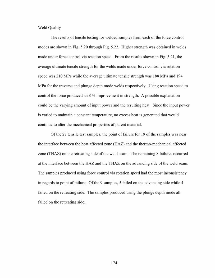
174

Weld Quality

The results of tensile testing for welded samples from each of the force control

modes are shown in Fig. 5.20 through Fig. 5.22. Higher strength was obtained in welds

made under force control via rotation speed. From the results shown in Fig. 5.21, the

average ultimate tensile strength for the welds made under force control via rotation

speed was 210 MPa while the average ultimate tensile strength was 188 MPa and 194

MPa for the traverse and plunge depth mode welds respectively. Using rotation speed to

control the force produced an 8 % improvement in strength. A possible explanation

could be the varying amount of input power and the resulting heat. Since the input power

is varied to maintain a constant temperature, no excess heat is generated that would

continue to alter the mechanical properties of parent material.

Of the 27 tensile test samples, the point of failure for 19 of the samples was near

the interface between the heat affected zone (HAZ) and the thermo-mechanical affected

zone (THAZ) on the retreating side of the weld seam. The remaining 8 failures occurred

at the interface between the HAZ and the THAZ on the advancing side of the weld seam.

The samples produced using force control via rotation speed had the most inconsistency

in regards to point of failure. Of the 9 samples, 5 failed on the advancing side while 4

failed on the retreating side. The samples produced using the plunge depth mode all

failed on the retreating side.

175

Tensile Test Results - Force Control via Traverse Speed

0

50

100

150

200

250

Sample

1a

Sample

1b

Sample

1c

Sample

2a

Sample

2b

Sample

2c

Sample

3a

Sample

3b

Sample

3c

Sample Number

Strength (MPa) .

Ultimate Strength (Mpa) Fracture Strength (Mpa)

Figure 5.20: Tensile test results from force control via traverse speed.

Tensile Test Results - Force Control via Rotation Speed

0

50

100

150

200

250

Sample

1a

Sample

1b

Sample

1c

Sample

2a

Sample

2b

Sample

2c

Sample

3a

Sample

3b

Sample

3c

Sample Number

Strength (MPa) .

Ultimate Strength (Mpa) Fracture Strength (MPa)

Figure 5.21: Tensile test results from force control via rotation speed.

176

Tensile Test Results - Force Control via Plunge Depth

0

50

100

150

200

250

Sample

1a

Sample

1b

Sample

1c

Sample

2a

Sample

2b

Sample

2c

Sample

3a

Sample

3b

Sample

3c

Sample Number

Strength (MPa) .

Ultimate Strength (Mpa) Fracture Strength (Mpa)

Figure 5.22: Tensile test results from force control via plunge depth.

Marco cross sections shown in Fig. 5.23 through Fig. 5.25 are absent of weld

flaws such as internal voids or worm holes. These results indicate that changing the

traverse speed, rotation speed or plunge depth during the welding operation, did not

adversely affect the weld quality. It is worth noting that using plunge depth as the

controlling variable produced the least amount of weld flash since the tool was able to

adjust to the work piece’s surface.

Figure 5.23: Cross section of weld produced under traverse force control mode.

177

Figure 5.24: Cross section of weld produced under rotation force control mode.

Figure 5.25: Cross section of weld produced under plunge depth force control mode.

Conclusions

With force control via traverse speed and force control via rotation speed, the

controller can not adjust the tools plunge depth. The controller alters the axial force

through thermo-mechanical means. Therefore if the work pieces has minimum variation

and the machine being used to apply the weld is very stiff, these methods of force control

provide an attractive alternative to force control via plunge depth.

Force control via traverse speed varies the distribution of heat along the weld

seam to maintain a constant force. Since axial force is an excellent indicator of the

relative temperature beneath the weld tool, it is hypothesized that a constant temperature

is maintained in the welding environment. It is concluded that weld seam heat

distribution control is a byproduct of force control via traverse speed.

178

Force control via rotation speed changes the rate of heat generation in order to

control the axial force. With this method of force control, the amount of weld power is

continuously varied to maintain the desired force.

Force control via plunge depth uses physical contact between the tool and the

work piece as the controlling variable. This method is the most difficult to control due to

the metal flow dynamics associated with the vertical movement of the tool. To

successfully implement force control via plunge depth four key enablers were identified.

These key enablers involve reducing the sensitivity of the interaction between the tool

and the work piece. When these enablers are implemented, the system is able to maintain

stability.

The presented energy model supports the hypothesis of heat distribution control

along the weld seam when force control via traverse speed is used. It could also be used

to support the same hypothesis when force control via rotation speed is used, but the level

of control is not as refined. It is also noted how nearly constant power is maintained with

force control via plunge depth.

Understanding the contributing effect each of these variables has on the force is

important to establishing a stable manufacturing system. Historically force control has

been achieved using plunge depth as the controlling variable. As noted above, this mode

of force control is susceptible to stability issues if not configured correctly. However if

relatively stiff machine tools or selectively compliant assembly robot arms (SCARA) are

used, force control via traverse speed and rotation speed provide attractive alternatives.

Force control via traverse speed and rotation speed are more stable and can effectively

179

maintain a constant force when there is a minimum amount of work piece variation

present.

Future work can be directed on combining these modes of force control in an

effective manner. Each has its own merits and could be used in certain situations. As an

example, large changes in force due to robot deflection or material variation should be

addressed with plunge depth while thermal changes in the welding environment are better

suited for traverse speed changes.

180

CHAPTER VI

TORQUE CONTROL OF FRICTION STIR WELDING FOR MANUFACTURING AND AUTOMATION

William R. Longhurst, Alvin M. Strauss, George E. Cook, Paul A. Fleming

International Journal of Advanced Manufacturing Technology. Current Status:

Submitted June 17, 2009 and under review.

Abstract

Friction Stir Welding (FSW) is a solid state welding process that utilizes a

rotating tool to plastically deform and forge together the parent materials of a work piece.

The process involves plunging the rotating tool that consists of a shoulder and a pin into

the work piece and then traversing it along the intended weld seam. The welding process

requires a large axial force to be maintained on the tool. Axial force control has been

used in robotic FSW processes to compensate for the compliant nature of robots.

Without force control, welding flaws would continuously emerge as the robot

repositioned its linkages to traverse the tool along the intended weld seam. Insufficient

plunge depth would result and cause the welding flaws as the robot’s linkages yielded

from the resulting force in the welding environment.

The research present in this paper investigates the use of torque instead of force to

control the FSW process. To perform this research, a torque controller was implemented

on a retrofitted Milwaukee Model K milling machine. The closed loop proportional,

181

integral plus derivative (PID) control architecture was tuned using the Ziegler-Nichols

method. Welding experiments were conducted by butt welding ¼ inch (6.35 mm) x 1 ½

inch (38.1 mm) x 8 inch (203.2 mm) samples of aluminum 6061 with a ¼ inch (6.35 mm)

threaded tool.

The results indicate that controlling torque produces an acceptable weld process

that adapts to the changing surface conditions of the work piece. For this experiment, the

torque was able to be controlled with standard deviation of 0.231 Newton – meters. In

addition, the torque controller was able to adjust the tool’s plunge depth in reaction to 1

millimeter step and ramp disturbances in the work piece’s surface. It is shown that torque

control is equivalent to weld power control and causes a uniform amount of energy per

unit length to be deposited along the weld seam.

It is concluded that the feedback signal of torque provides a better indicator of

tool depth into the work piece than axial force. Torque is more sensitive to tool depth

than axial force. Thus it is concluded that torque control is better suited for keeping a

FSW tool properly engaged with the work piece for application to robotics, automation,

and manufacturing.

Introduction

Friction Stir Welding (FSW) is a material joining process that was invented by

Wayne Thomas of The Welding Institute (TWI) and patented in 1995 (Thomas et al.

1995). During the joining process the parent materials remain in their solid state unlike

fusion welding processes that require the parent materials to be melted. Because the

parent materials remain in the solid state, FSW offers many advantages over fusion

182

welding processes. These advantages include reduced porosity, increased mechanical

strength, no filler material or welding fumes. Primarily FSW is used to join metals with

low melting points such as aluminum and copper.

The FSW process utilizes a rotating non-consumable tool to perform the welding

process. In its simplest form the rotating tool consists of a small pin (or probe)

underneath a larger shoulder. Metal flow caused by the tool is very complex and is an

area where a great deal of research is ongoing. One accepted model that provides insight

into the metal flow phenomena and the resulting joining of the parent metals is the

Arbegast model (Schneider 2007). Arbegast’s model of metal flow describes five zones

within the welding process. The five zones are: preheat, initial deformation, extrusion,

forging and lastly the cool down. The preheating of the metal occurs due to the transfer

of heat ahead of the traversing tool. The initial deformation occurs as the soften metal

ahead of the tool begins to deform due to the rotation of the tool. Next, as the tool

advances into the heated and slightly deformed metal, the rotating pin extrudes the metal

around to the backside of the pin where it is subjected to high forging pressure from the

shoulder. Once the metal has been extruded to the backside of the pin and forged

together, it has undergone serve deformation but has remained in its solid state. As the

newly forged metal exits from underneath the backside of the shoulder it begins to cool

either naturally or through some forced convection method. Figure 6.1 illustrates the

FSW process as described by Arbegast’s model.

183

Figure 6.1: FSW Process (Wikipedia 2009).

Historically there have been three process parameters used to control FSW during

steady state conditions. They are the FSW tool’s plunge depth, rotation rate and traverse

rate. However, as FSW evolved from its infancy, the axial force placed on the work

piece by the tool became a very important process parameter. The reason for its

emergence as an importance parameter is linked to the application of FSW with robots.

Similar to other welding technologies, the application of FSW with robots provides a

very flexible platform for automation. However, with FSW the relatively large forces

present a challenge. The load bearing capability of robots is limited and thus most robots

are not well suited for FSW. In addition their compliant nature makes FSW much more

challenging.

To address the compliance problem, force control has been presented as a

solution. With robotic FSW the challenge is to keep the tool positioned correctly with

adequate force on the tool, while the linkages of the robot continually reposition

themselves. The motion of the linkages, along with their reaction to the large welding

forces, results in positioning errors of the tool. In conjunction with these positioning

errors, large fluctuations in the forging force results within the welding environment.

184

These positioning errors and force fluctuations will possibly lead to insufficient

deformation, forging and consolidation of the parent metals. With force control, constant

axial force is maintained on the tool and the likelihood of welding flaws is diminished.

Successful applications of robotic FSW have been documented with work by

Smith (2000), Soron and Kalaykov (2006), and Zhao et al. (2007). Each of these groups

developed and implemented a force control architecture using plunge depth as the

controlling variable. All were able to conclude it was feasible to implement FSW force

control architectures. However, force control of FSW remains difficult and its operation

confined to a limited range of process parameters due to the highly nonlinear welding

environment. Smith used a force control architecture based upon a Jacobian relationship

between motor torques and welding forces (Craig 2005). He was successful but the

controller was stable for a limited range of process parameters and a controller update

frequency of less than 2 Hz. Soron and Kalaykov concluded that even with the added

force control to the robotic FSW system, axial force oscillations still exist when the tool

makes contact with the material. They also note the penetration depth is hard to predict

due to the positioning error of the robot. Zhao et al. presented a non-linear axial force

controller they developed and implemented for a FSW process. They were able to

experimentally model the static and dynamic behavior of the interaction between the

FSW tool and the work piece. With this information and using an open architecture

control system they were able to design a controller using Polynomial Pole Placement.

Good results were obtained, but to handle the non-linear transient response when the

tool’s plunge depth changed, the control system had to incorporate experimentally

185

obtained dynamic parameters. Thus the controller’s parameters were specific to their

experimental setup.

Even with these advances the problems associated with robotic FSW are not

solved. As noted by Soron and Kalaykov, problems still exists with force oscillations.

The highly non-linear aspect of the welding environment makes it extremely difficult to

implement a robust system that maintains stability over a large range of process

configurations and parameters.

Research by Fleming (2009) introduces the potential for torque as a feedback

signal for seam tracking of FSW lap weld joints. His work on other tracking algorithms

had used axial force as the feedback but a high amount of noise in the force signal caused

him to explore torque as the feedback signal. A similar situation could be present with

force control of FSW?

The research presented in this paper introduces and examines torque as a

controlled parameter instead of axial force. A torque control architecture that varies

plunge depth to maintain a desired torque is implemented on a three axis milling

machine. The resulting performance of the torque controller is analyzed and

relationships between axial force and torque are defined. Features are identified that

make torque control more attractive than force control. It is concluded that controlling

the torque provides a better indication of plunge depth than force.

Experimental Setup

The experiment was conducted on the FSW system at Vanderbilt University

which is shown in Fig. 6.2. The FSW system is a Milwaukee Model K milling machine

186

that has been retrofitted with more advanced motors and instrumentation. These retrofits

were previously added to automate the system and provide a programmable platform for

FSW experimentation. At the top of the control hierarchy is a master computer that

enables all of the systems subcomponents such as the motor drive controllers and

instrumentation. The master computer is a Dell Precision 340 that uses Microsoft

Windows XP as its operating system. The welding and torque control code was written

in C#. A graphical user interface within the C# software allows the operator to select the

desired welding parameters for the pending operation. These parameters include the

FSW tool’s rotation speed, traverse speed, plunge depth and weld path position.

Figure 6.2: FSW machine at Vanderbilt University.

The tool’s z axis coincides with the milling machine worktable’s vertical axis

when the tool is at a zero degree tilt angle. The worktable resides on the knee that is

187

mounted to a vertical positioning screw and secured in sliding dovetail joints. The knee

travels on the screw via a gear system inside the knee. An externally mounted belt and

pulley system is attached to the input shaft of the gear system. Power is provided by a

Parker Compumoter KH series brushless servo motor. The servo motor is controlled by a

Parker Compumotor KHX-250 servo drive that utilizes a proportional, integral plus

derivative (PID) control algorithm. Command signals are sent directly from the master

computer to the servo drive. Vertical position of the table is obtained from a Reinshaw

linear scale that has a resolution of 10 micrometers. Position data from the sensor is fed

into a sensor box were it is converted to a digital signal prior to being sent to the master

computer.

Welding force data is collected through a Kistler Rotating Cutting Force

Dynamometer. The dynamometer collects x-axis force, y-axis force, z-axis force as well

as the torque about the z-axis. The analog signal from the dynamometer is sent to a signal

conditioning box where it is converted from an analog signal to a digital signal. Once

converted the data is sent to a separate computer where the data is sorted, recorded and

displayed before being sent to the master computer.

An overview of the closed loop torque control system is illustrated in the control

block diagram of Fig. 6.3. Within the master computer a desired torque is selected. The

desired torque value is subtracted from the actual torque value to obtain a torque error.

The torque error signal is then processed in the control law. The servo drive produces a

change in the vertical position of the tool which results in a change of the torque acting

on the tool. The dynamometer reads the resulting torque and returns it to the master

computer where it is once again compared to the reference signal.

188

Figure 6.3: Block diagram of torque control via plunge depth.

The servo motor operates in a continuous mode and turns the output shaft based

upon the value of the processed error signal. For this mode of operation, velocity and

acceleration profiles were preprogrammed for complete motion control of the output

shaft and the movement of the FSW tool. For the experimental setup a motion profile

was chosen that resulted in the system having smooth acceleration and deceleration. This

increased the stability of the torque controller by reducing the magnitude of the transient

torque response of the system. A trapezoidal velocity profile was chosen and

preprogrammed into the torque controller. With the trapezoidal profile, the acceleration

was always constant at the beginning and end of the motion. The torque controller would

determine the amount of the torque error, process the error signal according to the control

law and send a motion command to the servo drive. The preprogrammed motion profile

was scaled by the torque controller to the size of the processed error signal before being

sent to the servo drive.

189

The measured torque signal was very noisy. This noise makes the process of

applying derivative control to the system very difficult. The noise would simply be

amplified by the controller. To address this problem, a filter was implemented. The filter

is a five point moving average of the torque with an interrupt frequency of 3.33 Hz. For

this experimental setup these filter parameters were found to provide adequate noise

reduction without adding too much phase lag in the signal.

To create and investigate the performance of torque control via plunge depth, a

PID control architecture was chosen. To tune the PID torque controller and achieve

optimum control, the Ziegler-Nichols tuning method was used (Ogata 2002). The

Ziegler-Nichols tuning method called for the controller to use only proportional control

while welding. While using proportion control only, a critical gain value was

experimentally determined through trial and error. Over the course of several welds, the

gain was steadily increased until the resulting torque achieved sustained oscillation. The

sustained oscillation constituted marginally stable behavior. The resulting control gain

and time period between oscillations was recorded and used to calculate PID gains for the

controller. The resulting PID control law is shown in Eq. (6.1). In Eq. (6.1), Kp is the

proportional gain, Ki is the integral gain, Kd is the derivative gain, e is the error and u is

the resulting control signal as a function of time t.

Kp e + Ki ∫e + Kd e΄ = u(t) (6.1)

For this torque control research, a ¼ inch (6.35 mm) treaded tool was selected. A

picture of the tool is shown in Fig. 6.4. The threaded pin was 0.235 inches (5.969 mm)

190

long with a diameter of 0.250 inches (6.35 mm) across its threads. The shoulder was of a

hybrid nature. It had a flat 0.625 inch (15.875 mm) diameter shoulder that acted as the

forging surface. The remaining portion of the shoulder was on a 7° taper that started at

the 0.625 inch (15.875 mm) diameter point and continued to the 1 inch (25.4 mm)

outermost diameter. The tool was positioned on a 1° lead angle relative to the work

piece. From the Ziegler-Nichols tuning method, the critical gain and period for the ¼

inch threaded tool was 8.6 and 11.0 seconds. The resulting control gains are shown in

Table 6.1.

Figure 6.4: FSW tool used for torque control.

Table 6.1: Torque control gains.

For the experiment ¼ inch (6.35 mm) butt welding with full penetration was

performed. The material used was aluminum 6061. The work piece consisted of two ¼

191

inch (6.35 mm) by 1 ½ inch (38.1 mm) by 8 inch (203.2 mm) long samples. Each weld

began with the tool plunging into the metal 1 inch (25.4 mm) from the end of the work

piece. Once the tool achieved the desired plunge depth it dwelled at that location for 5

seconds in order to soften the work piece by generating additional heat. After dwelling,

the tool began to traverse forward at either 6 inches per minute (IPM) (152.4 mm per

minute) or 3 IPM (76.2 mm per minute). After traversing 1 inch (25.4 mm) the torque

controller was engaged. The torque controller was operating in a regulation mode,

meaning whatever the torque was at the time of engagement, was the selected desired

torque. The system operated under torque control mode until it reached 1 inch (25.4 mm)

from the end of the 8 inch (203.2 mm) work piece. Thus 5 inches (127 mm) of welding

was conducted each time under torque control. For every weld made, the tool’s shoulder

was initially plunged between 0.000 – 0.002 inches (0.000 -0.051 mm) below the surface

and the tool’s rotation rate was maintained at a constant 1400 revolutions per minute

(RPM).

Results and Discussion

The resulting torque can be seen in the data of Fig. 6.5. As the tool slowly

plunged into the work piece, the torque steadily increased. The plunged began at

approximately 120 seconds and ended at 220 seconds. At the end of the plunge the tool

dwelled for 5 seconds. While the tool was dwelling, the torque slowly decreased about 2

½ Newton-meters (N-m). Once the dwelling was complete the tool began traversing

forward. As the tool began to move forward a relatively large spike in torque occurred.

However the torque returned to its original value after about 5-7 seconds. The most

192

probable cause of this transient response was the built up ridge of material surrounding

the tool from its initial plunge into the work piece. The tool must travel through this

ridge during the first few seconds of forward movement.

After 1 inch (25.4 mm) of forward travel, the torque control is engaged. The

torque control engagement is noted by the desired torque curve in Fig. 6.5. As can be

seen in Fig. 6.5 the torque is regulated to the desired value. This torque is maintained

until the end of the weld. At the end the tool is retracted from the work piece.

120 140 160 180 200 220 240 260 2800

5

10

15

20

25

Torque (Newton - Meter) as a Function of Time (seconds)

P Control, 1/4" Threaded Tool

Torque (N-m)

Time (sec)

Actual Torque

Desired Torque

Figure 6.5: Torque controlled response.

The results of Fig. 6.6 provide more detail into the performance of the torque

controller. A close-up view of the torque curve during torque control is present.

193

Statistical analysis reveals the controller was able to obtain a mean torque of 15.57 N-m

with a standard deviation of 0.231 N-m. The desired torque the controller was trying to

obtain was 15.52 N-m. The range of torque was 1 N-m with a maximum value of 15.98

N-m and a minimum value of 14.98 N-m. The median value was 15.6 N-m.

230 235 240 245 250 255 260 265 270 2750

5

10

15

20

Torque (Newton - Meter) as a Function of Time (seconds)

P Control, 1/4" Threaded Tool

Torque (N-m)

Time (sec)

230 235 240 245 250 255 260 265 270 2755.456

5.458

5.46

5.462

5.464Verticle Position (inches) as a Function of Time (seconds)

Ver Position (in)

Time (sec)

Actual Torque

Desired Torque

Figure 6.6: Regulation of the torque.

To control the torque, the plunge depth had to be adjusted over a range of

approximately 0.005 inches (0.127 mm). The position of the worktable is shown below

the torque data in Fig. 6.6. The first adjustment was the retracting of the tool to reduce

the plunge depth. As the tool approached the end of the work piece the torque had to be

increased two separated times by plunging the tool deeper into the work piece. Since the

194

work piece was flat, the adjustments can be attributed to the changing thermal conditions

within the work piece and not physical changes in the work piece’s surface. The first

adjustment occurred to reduce the torque as the tool was moving into a colder weld

region. The last two adjustments were needed to increase the torque because the welding

environment had grown softer due to the build up of heat near the end of the work piece.

Using axial force control instead of torque control produces similar results. It is

difficult to compare the two methods statistically since the outputs have different units,

but qualitatively they can be compared. The most notable similarity is the amount of

adjustment in plunge depth needed. Force control experiments conducted with this same

FSW equipment required a range of 0.005 inches (0.127 mm) in adjustment to maintain a

desired force. As evident from the data in Figure 6.6, this proved to be the same case

with torque control. The same can be said about the adjustment to the step disturbance.

Both force and torque control required the same amount of plunge depth adjustment to

1millimeter step disturbances.

When the FSW system is operating under torque control, a constant amount of

power is input into the welding environment. In a sense, energy control emerges as a by-

product of torque control. This is evident by the results shown in Fig. 6.7. In Fig. 6.7,

the input power (Watts) and the energy per unit length of weld (Joules per millimeter) is

defined by Eq. (6.2) and Eq. (6.3). In these equations, P is the power, Ft is the traverse

force, vt is the traverse velocity, M is the torque and ω is the tool rotation speed.

P = (Ft x vt) + (M x ω) [Watts] (6.2)

E = P / vt [Joules / mm] (6.3)

195

With welds made at low speed, a large majority of the input power is due to the

torque and rotation speed. When constant torque is maintained by the controller, the

input power and energy per unit length of weld is approximately constant as well. The

small variation is attributed to the small variation of the torque and the traverse force.

230 235 240 245 250 255 260 265 270 27510

15

20Torque (Newton - Meter) as a Function of Time (seconds)

Torque (N-m)

Time (sec)

230 235 240 245 250 255 260 265 270 275

1000

2000

3000

Input Weld Power (Watts) as a Function of Time (seconds)

Time (sec)

Weld Power (W)

230 235 240 245 250 255 260 265 270 275600

800

1000

1200Weld Seam Energy (Joules / Millimeter) as a Function of Time (seconds)

Time (sec)

Energy (J / mm)

Figure 6.7: Energy model of FSW while under torque control.

The torque controller’s response to physical changes on the work piece surface is

shown in Fig. 6.8 through Fig. 611. Figure 6.8 shows the response to a 1 millimeter step

change in thickness of the work piece. The welded sample with the 1 millimeter step can

be viewed in Fig. 6.9.

As the tool traversed across the surface, it encountered the torque disturbance. To

reject the disturbance and return the torque back to its desired value, the worktable had to

196

move downward 1 millimeter. As can be seen in Fig. 6.8 the controller successfully

accomplished this. It took the controller approximately 25 seconds to adjust to the

change in the work piece’s surface.

230 240 250 260 270 280 2900

5

10

15

20

Torque (Newton - Meter) as a Function of Time (seconds)

P Control 1/4" Threaded Tool, 1mm Step Disturbance

Torque (N-m)

Time (sec)

230 240 250 260 270 280 290

5.42

5.44

5.46

Verticle Position (inches) as a Function of Time (seconds)

Ver Position (in)

Time (sec)

Actual Torque

Desired Torque

Figure 6.8: 1 millimeter step disturbance.

Figure 6.9: Weld sample with 1 millimeter step.

197

The response to a ramp disturbance is shown in Fig. 6.10 and Fig. 6.11. To create

the disturbance the work piece was placed on an incline. The incline resulted in one end

of the work piece being 1 millimeter higher than the other. The resulting force and

worktable position are shown in Fig. 6.10. The controller adjusted the tool’s position

quite well and maintained a nearly constant torque over the course of the weld.

220 240 260 280 300 320 3405

10

15

20

25

Torque (Newton - Meter) as a Function of Time (seconds)

P I Control, 1/4" Threaded Tool, 1mm Slope Disturbance

Torque (N-m)

Time (sec)

220 240 260 280 300 320 3405.6

5.61

5.62

5.63

5.64

Verticle Position (inches) as a Function of Time (seconds)

Ver Position (in)

Time (sec)

Actual Torque

Desired Torque

Figure 6.10: 1 millimeter ramp disturbance.

Figure 6.11 is a picture of the welded work piece that was position on an incline.

The resulting weld is void of excess weld flash, thus indicating the controller was able to

adjust the tool to the continuously changing work piece’s surface. Without torque control

198

this would not be possible. To illustrate the difference, a weld was made with the work

piece on the identical incline, but without the use of torque control. The results are

shown in Fig. 6.12. As can be seen, an excessive amount of flash was generated due to

the tool digging into the material and not adjusting to the changing work piece’s surface.

Figure 6.11: Weld sample with 1 millimeter ramp.

Figure 6.12: Weld sample with 1 millimeter ramp and no torque control.

To investigate the relationship between axial force and torque, the torque data in

Fig. 6.5 is shown again in Fig. 6.13, but with the corresponding axial force. During the

region of control, the force follows the same trend as the torque. When the torque

decreases, so does the force. Likewise when the torque is increased, the force increases.

199

However there is a very distinct difference in torque and force during the initial plunge of

the material.

Notice in Fig. 6.13 how the torque steadily increases as the tool is plunged into

the work piece. This is occurring between the times of 120 seconds to 220 seconds. In

contrast the force is not steadily increasing. The force curve has three distinct regions.

The regions are; the initial rise in force due to the pin contacting the work piece, the

reduction in force as the pin continues to plunge and the increase in force due to the

shoulder contacting the work piece. What is interesting about this comparison is the fact

that torque is more representative of the actual plunge depth.

120 140 160 180 200 220 240 260 280

2000

4000

6000

8000

10000Z-Force (Newtons) as a Function of Time (seconds)

Z-Force (N)

Time (sec)

120 140 160 180 200 220 240 260 2800

5

10

15

20

25Torque (Newton - Meter) as a Function of Time (seconds)

Torque (N-m)

Time (sec)

Actual Torque

Desired Torque

Acutal Force

Ref. Force

Figure 6.13: Recorded torque and force during welding.

200

To understand why torque is more closely related to the plunge depth lets look at

the mathematical definition of torque as given by Nunes et al. (2000). Nunes uses a

rotating plug model to develop the equation for torque. He theorizes a small volume of

material sticks and rotates with the tool. According to Nunes, shearing of the work piece

occurs at a shear interface boundary and not at the tool’s surface. The pressure needed

for shearing and subsequent deformation at the interface boundary is simply the shear

flow stress σ. Approximating the surface of the shear interface boundary as the surface

of the tool, the torque M, can be computed with Eq. (6.4).

M = Torque on Shoulder + Torque on Pin Sides + Torque on Pin Bottom =

(6.4)

In Eq. (6.4), R is the radius of the shoulder, r is the radius of the pin, t is the

length of the pin and σ is the shear flow stress. The resulting torque in Fig. 6.13 can be

explained by using Eq. (6.4). At the moment of contact between the bottom of the pin

and the work piece, the torque quickly rises. The torque at this point is only acting on the

bottom of the pin. Thus the third part of Eq. (6.4) is used to determine the torque. Since

the bottom of the pin is flat, it only takes a few seconds for the bottom of the pin to be

submerged below the surface and hence the sharp increase in torque at the beginning of

the plunge. The steady increase in torque is attributed to the second portion of Eq. (6.4).

The second portion of the equation defines the torque along the sides of the pin. Its

value is directly proportional to the depth of the pin into the work piece. Thus this can

explain the steady and rather linear increase in torque as the tool is plunged further into

201

the work piece. At the end of the plunge there is a noticeable increase in torque. This is

due to the shoulder contacting the work piece. Mathematically it can be explained with

the addition of the first portion to the overall value of the torque.

Torque is also a function of the shear flow stress of the work piece. The shear

flow stress is temperature dependent, thus as more heat is generated and the work piece

becomes softer, the shear flow stress reduces. However upon comparison, torque appears

to be less sensitive to thermal conditions than does force. In addition, a change in axial

force is dependent upon a change in the amount of tool surface area in contact with the

work piece. For instance, as the pin continues its path downward into the material during

the initial plunge, there is no further change in tool surface area perpendicular to the axial

direction. Once the bottom of the pin is submerged, no further changes occur until the

shoulder reaches the surface of the work piece. With no change in surface, there is no

increase in force. The additional heat added during the plunge reduces the force as the

pin is plunged. Thus using force to predict tool depth is not advised. However using

torque to predict tool depth does have potential.

Lastly, in the absence of a commercial force sensor such as a dynamometer,

torque can be easily measured with strain gages attached to the tool. Measuring the

elastic twisting of the tool is much more viable than trying to measure the axial

deformation. The axial deformation will be greatly affected by thermal expansion

whereas deflection due to torsion will not be as sensitive to an elevated temperature. As

another possibility, the torque acting on the tool could be obtained by measuring the

current used to power the spindle motor.

202

Conclusions

From the results it is concluded that using torque control is an attractive

alternative to force control. It is attractive because of its sensitivity to tool depth into the

work piece. When articulated arm robots are used for FSW, the control algorithm must

accommodate for deflection and positioning errors of the robot. In the past, force control

has been used to accomplish this task. However, due to the highly nonlinear relationship

between axial force, and the process parameters of plunge depth, rotation speed and

traverse speed, the use of force control is restricted to a range of processing parameters.

Torque control has the potential to increase the range of processing variables

suitable for stable control. Preliminary results from other experimentation at Vanderbilt

University supports the conclusion that torque control is more attractive. FSW of pipe

and pressure vessel sections using a rotary positioning device in place of the traverse axis

was setup on the same FSW system described earlier. Using force control to adjust to the

concentricity of the parts and the deflection of the rotary device, circular seam welds

were produced. However this rotary setup created abnormally hot welding conditions.

With the circular configuration of the parts, the heat was trapped in the work piece and

could not conduct away from the work piece. As the heat continued to build within the

work piece, the stiffness of the welding environment changed drastically over the course

of the seam weld. Near the end of the weld, force control was not working effectively.

The tool would tend to dig into the material with no relative change in force realized.

However when torque control was used, a more desired response occurred. The tool was

better able to track the surface of the work piece as it rotated one complete revolution.

203

Torque control also provides a method to control the weld power. Since weld

power is predominately a function of torque and tool rotation speed, the input power

remains constant under torque control. Along with constant input power, a uniform

amount of energy per unit length of weld is deposited into the weld seam.

Future work could attempt to quantify the range of process variables for stable

torque control. In addition, work could be performed to see which tool geometries work

best with torque control. A flat shoulder creates a more sensitive region where a very

small change in plunge depth will produce a relatively large change in torque. An

increased lead angle could create more stable control systems by eliminating the large

and relatively instantaneous change in torque associated with a flat shoulder.

More importantly, work can be done to develop a measurable correlation between

tool depth and torque. There would be great potential for use of torque as a feedback

signal indicating tool depth. Until a measurable correlation can be established, the

combined use of force and torque control should be exploited for maximum robustness of

robotic FSW systems. A possible course of direction would be to control torque as cited

in this paper while monitoring the force. If the axial force exceeded pre-established

limits, a process alarm could be generated indicating the possibility of a welding flaw.

Both axial force and torque are important regarding the production of quality welds, but

torque would be better suited as the primary parameter to control due to its sensitivity of

tool depth. Controlling torque has great potential for the advancement of FSW in

manufacturing and automation.

204

CHAPTER VII

LAP WELDING UNDER FORCE CONTROL

Introduction

Lap welds present a different set of challenges than does butt welds. The faying

surface is perpendicular to the vertical axis of the FSW tool for lap welds where in butt

welds the faying surface in parallel. Typically laps welds are made with parent metals

that are relatively thin as compared to their width and length. The overlaying surfaces

typically do not fit together perfectly to create a flush fit-up. The relatively thin material

is not perfectly flat due to warping during its manufacturing process. This causes the

metal fit-up condition to typically be less than ideal. In addition, imperfect clamping can

lead to warping and bending of the pieces. These gaps create challenges for the FSW

process.

If position control is utilized for lap welding, the gaps between the parent metals

might lead to wormholes or other flaws. If the plunge depth is set at point where a gap

exists, as the tool travels forward the shoulder could disengage from the work piece. As

the shoulder disengages, the forging pressure is reduced and flaws emerge.

Force control creates a flexible welding system that is able to adapt to the

imperfect metal fit-up and create a quality weld. The controller will ensure that a large

enough force is applied so as to squeeze together the two pieces that comprise the work

piece. Talwar et al. (2000) stated that “Successful friction stir welding (especially for lap

joints) requires welding under force control.”

205

Experimental Setup

Two 1/8 inch thick by 3 inches wide by 8 inches long samples were stacked

together and lap welded using a ¼ inch threaded FSW tool. The tool was plunged 1 inch

from the end of the work piece and from that point the tool traversed forward 6 inches

before being extracted. The force controller was engaged after 1 inch of travel. The tool

was placed on a 1° lead angle and the back edge of the shoulder was plunged 0.002

inches below the surface of the work piece. The tool rotated at 1400 RPM and traversed

forward at 6 inches per minute. Based upon pervious weld experience a desired welding

force of 6000 Newtons was selected. The welding was conducted on a Milwaukee model

K milling machine that utilized a Kistler Dynamometer for force measurements.

Results

The results of the lap welding can be seen in Figure 7.1 and 7.2. In Figure 7.1 the

force and table position data. The initial plunge of the tool is completed just past 220

seconds. At that point the force is just below 6000 N. Prior to traversing forward the tool

dwells for 5 seconds. As the tool begins to move forward, the force increases for a few

seconds before it drops to 4000 N. During this time the weld is under position control.

As can be seen Figure 7.2, a worm hole developed during this operation. After the 1 inch

of travel was complete the force controller was engaged. As can be seen in Figure 7.1 the

force quickly increase to 6000 N and was maintained for the remaining duration of the

weld. When the force increased the worm hole was eliminated as shown in Figure 7.2.

206

220 230 240 250 260 270 280 290 3002000

4000

6000

8000Z-Force (Newtons) as a Function of Time (seconds)

Z-Force (N)

Time (sec)

220 230 240 250 260 270 280 290 3004.92

4.93

4.94

Verticle Position (inches) as a Function of Time (seconds)

Ver Position (in)

Time (sec)

Actual Force

Desired Force

Figure 7.1: Force control data of lap weld.

Figure 7.2: Lap weld with force control.

207

Conclusions

It can be concluded that force control corrects for the imperfect metal fit-up

conditions that may exist for lap configurations. When a substantial enough force is

applied the two pieces that define the work piece are squeezed together. This squeezing

action collapses the voids that may exist in the welding environment and forges together

the deformed metal in a single solidified joint. This process can be compared to the

pressure needed for resistive spot welding. With resistive spot welding an adequate

amount of force is needed to squeeze together the pieces of metal in order to create a

good contact condition for current to flow thought the work piece.

Even though there were no geometry changes in the surface of the work piece,

force control of FSW was needed to produce a quality weld. Future research can be

conducted that utilizes real time monitoring techniques to adjust the amount of force to

ensure no worm holes are present.

208

CHAPTER VIII

CONCLUSION AND FUTURE WORK

Conclusion

Force control of FSW can be accomplished by using the tool plunge depth,

traverse speed or rotation speed as the controlling variable. Each variable contributes to

the axial force in a unique way. The plunge depth increases or decreases the force

through physical contact with the work piece. Changing the rotation speed of the tool,

changes the rate of heat generation which in turn changes the force. When the tool’s

traverse speed changes, a different amount of heat is applied per unit length of weld

seam. Each of these controlling variables has its advantages as well as disadvantages.

As an alternative to controlling the force, torque control provides a method of control that

is more sensitive to plunge depth. This increase in sensitivity has been shown to be more

effective in maintaining proper tool contact with the work piece during abnormally hot

welding conditions.

The most potential for force control lies in the application of FSW through

robotics. Since robots are compliant in nature and subject to linkage deflection, force

control provides a viable method for robotic FSW. Without force control, robotic FSW

would be an extremely challenging situation. The tool’s shoulder would not stay

properly engaged with the work piece surface as the robot continually repositioned itself.

However force control solves this problem.

209

The results from Chapter II and Chapter IV show that using traverse speed instead

of plunge depth as the controlling variable provides greater accuracy in maintaining a

desired axial force. The main enabler for this accuracy is the unidirectional dynamics of

the drive motor. The traverse motor never has to stop and reverse its direction. To make

force corrections the motor’s speed is simply changed when directed by the controller.

Without having to stop and reverse itself, greater bandwidth and response times are

achieved as compared to a motor controlling plunge depth. The second enabler is load

dynamics which allow the drive motor and its VFD to be free of the large dynamic forces

associated with the axial force. These two items lead to lower bandwidth and reaction

times.

The conclusion that axial force control via traverse speed is better depends upon

the FSW system and the process setup. The welding experiments conducted at

Vanderbilt University were conducted on a three axis milling machine. Due to a constant

plunge depth, the worktable was fixed along the vertical axis during the welding

operation. The same results might not be achieved using certain types of robots. For

instance if a six axis jointed-arm robot is to control axial force via traverse speed, more

than one linkage must be adjusted simultaneously as the tool continuously traverses along

the weld seam. Any simultaneous multi linkage adjustment possibly could result in small

fluctuations of the tool’s plunge depth. This force control method probably would work

best when the robot’s linkages to be adjusted reside in a parallel plane to the weld seam.

The linkages could be adjusted via either a prismatic or revolute joints. Thus a SCARA,

a Cartesian robot or a gantry style machine tool would be a good candidate for supporting

force control via traverse speed.

210

Process setup also requires the condition of the welding surface to be relatively

constant. With the controlling variable of traverse speed, there is no means to adjust the

vertical position of the tool to changing surface conditions. This requires the plunge

depth of the tool to be set a position such that the tool’s shoulder will always be in

contact with the material. Essentially the plunge depth must be set as if the welding was

being conducted under position control.

It is hypothesized that heat distribution control is a byproduct of force control via

traverse speed. This hypothesis is based upon force being proportional to the temperature

of the work piece beneath the tool. The feedback signal of force provides a relative

measurement of temperature. If the temperature in the welding environment increases,

the force is reduced. If the temperature decreases, the force increases. By maintaining a

constant force, constant temperature is also maintained in the welding environment. This

leads to a constant welding temperature along the weld seam. The energy model

presented in Chapter IV supports this hypothesizes by qualitatively showing how the

input energy is constant while the deposited energy along the weld seam varies.

Force control via tool rotation speed is very similar to the traverse method. The

results from Chapter IV and Chapter V show the accuracy to the comparable to force

control via plunge depth but it utilizes the same thermo-mechanical relationship as the

traverse rate to maintain a desired force. Thus adjustments to material variation or robot

linkage deflection due to axial force are unattainable. However there is a noticeable

absent of the ill behaved transient force condition that is observed when the plunge depth

is used as the controlling variable. Thus it can be concluded that using rotation speed as

211

the controlling variable leads to a more stable control situation than when plunge depth is

used as the controlling variable.

One drawback to using rotation speed as the controlling variable was the amount

of weld flash present. Force control was not realized unless the entire shoulder was

submerged into the work piece. With the entire shoulder being in contact with the work

piece, no significant change in force occurred over the range of available rotation speeds.

However, flash can be minimized by using tools with features on their shoulders that

allow for a 0° lead angle. Features such as scrolls will enhance the metal flow, reduce

flash and produce acceptable welds at a 0° lead angle.

It is concluded that force control via rotation speed controls the axial force by

changing the rate of heat generation beneath the tool. Varying response to changing

rotation speed can be attributed to varying heat transfer conditions in near proximity to

the welding environment.

Using force control via plunge depth provides an intelligent architecture that is

able to adapt to changing work piece surface and thermal conditions. By adapting to

these changing conditions the tool is able to remain in contact with the material and

create adequate forging pressure. Without these conditions being met, welding flaws will

emerge. Without proper contact the tool will not generate enough heat nor will it

plastically deform the material to the extent required for welding. Without the proper

force the deformed material of the parent metals will not consolidate on the back side of

the pin. Either of these two conditions will cause severe flaws that lead to no weld

conditions.

212

Force control via plunge depth continually adjusts the tool to the optimized

position to minimize or eliminate weld flash. When setup correctly, the shoulder of the

tool will travel on the surface and not submerge itself completely. By staying on the

surface, a minimum amount of weld flash is generated. Since the weld flash is reduced to

a minimum, there is greater weld strength due to the thickness of the weld joint. Without

the use of force control, the weld joint thickness will vary and when more weld flash is

generated, the weld joint thickness is reduced. Thus force control provides a process that

increases the potential for greater load bearing capability of the resulting weld.

The disadvantage of force control via plunge depth lies within its controllability.

Although it can be stated that force control adds robustness to the weld process, the

controller can only function properly over a limited range of welding conditions. There

exists the potential for instability. The root of this instability can be traced to the highly

nonlinear welding environment. Changing thermal conditions, work piece stiffness,

transient force spikes and decaying force ripples create problems for the controller. The

controller must be setup correctly in order to provide a robust control platform.

For future implementations of FSW force control via plunge depth, four key

enablers have been identified from this research. The establishment and the adherence to

these key enablers will increase robustness and stability. The key enablers identified are:

• Maintaining a portion of the tool’s shoulder above the work piece surface.

• A smooth motion profile during plunge depth adjustment.

• Increasing the lead angle for flat shoulder tools.

• Establishing positional constraints.

213

Torque control is an attractive alternative to force control. It is attractive because

of its sensitivity to tool depth into the work piece. It also has the potential to increase the

range of processing variables suitable for stable control. Unlike axial force, equations

describing welding torque can be used to create models and provide insight into the

welding environment. These equations show in mathematical terms that torque is

directly proportional to the depth of the tool into the material. Results show that during

the plunge of the tool into the work piece, torque steadily increases while axial force

peaks prior to the tool being fully plunged into the work piece.

Torque control is also more attractive due to its simplicity. Instead of using

dedicated instrumentation such as a dynamometer, torque could simply be measured and

controlled via the spindle motor current. Using motor current as the feedback signal

would greatly reduce the cost and complexity of FSW systems.

Future Work

The presented work can be expanded in three different areas. The topics for

future work are: heat control as a byproduct of force control, real time process monitoring

and control, and the further development of torque control. Each of these topics can

enhance the overall development of force controlled FSW.

It was concluded in Chapter II that force control via traverse speed attempts to

maintain a constant temperature along the weld seam. This is accomplished due to the

relative relationship between force and temperature. If the force is maintained at a

constant value, so is the temperature. Further work can be done to determine the

accuracy of the heat control. The benefits of controlling the welding temperature would

214

allow for more uniform properties to exist within the weld seam. Perhaps an ideal

welding temperature could be established that maximizes the tensile strength?

An integrated system of process monitoring and force control could greatly

expand the range of parameters necessary for stable force control of FSW. An excellent

application would be for lap welds. As noted in Chapter VII force control is needed for

quality lap welds. The amount of force needed varies depending on the metal fit-up.

Metal fit-up issues arise when the imperfect surface conditions of the parent metals are

stacked or overlapped together. By applying enough axial force the imperfect fit-up

conditions at the faying surface can be overcome. Process monitoring could be used in

conjunction with force control to ensure the correct amount of force is being applied.

To possible methods of process monitoring are visual and force. With visual

detection of wormholes or flash the force could either be increased to eliminate the

wormhole or decreased to eliminate the flash. The visual sensor could be a laser that

scans the surface of the weld just behind the trailing edge of the tool. The laser would

have to have a fine enough resolution to detect the small voids at the surface of the weld.

With force monitoring wormholes could possibly be detected by monitoring the

amplitude and frequency of force fluctuations in a direction perpendicular to the direction

of tool travel. Research by Arbegast (2005) has shown a correlation between wormholes

and force fluctuation. The strong correlation exists when a high amplitude fluctuation

occurs at a low frequency.

From Chapter VI it was concluded that torque control has great potential for the

advancement of FSW in manufacturing and automation. It was discovered that torque

provides a good indication of plunge depth. Additional research should attempt to model

215

and quantify this relationship. With robotic FSW the tool must be properly plunged into

the work piece at all times. This is accomplished with force control because it can

compensate for the deflection of the robot. However the relationship between plunge

depth and axial force is highly nonlinear. In contrast the relationship between torque and

plunge depth is more proportional.

Along with modeling and further quantifying the relationship between torque and

plunge depth, simpler control systems could be developed. Using the spindle’s motor

current as a measure of the welding torque would be very valuable. Using the current as

the feedback signal would eliminate the need for any external instrumentation to directly

measure the torque. This would not only simplify the manufacturing setup but would

also lower the capital investment.

Another research topic that would further develop the use of torque control would

involve the investigation of how to desensitize the change in torque for a flat shoulder.

With a flat shoulder the torque rapidity changes with a very small change in plunge

depth. Since plunge depth is directly related to the torque value, this creates a region for

potential instability. From Chapter III it was shown that welding at increased lead angles

increases stability by desensitizing the interaction between the tool and the work piece. It

would be easier for robot programming and operations if the tool was always

perpendicular to the work piece surface. This possibly could be accomplished with a

convex shoulder that has scrolls on its surface? The convex shoulder would allow for a

portion of the shoulder to be above the surface thus maintaining stability while the scrolls

would enhance metal flow toward the pin. Future research could explore this and

determine if it is feasible to use torque control in this manner.

216

REFERENCES

Arbegast, W., Using Process Forces as a Statistical Process Control Tool for Friction Stir Welds., Friction stir welding and processing III; proceedings of a symposia held at the TMS annual meeting, San Francisco, California, Pages 193-204, 2005.

Atharifar, H., Dechao, L., Kovacevic, R., Numerical and Experimental Investigations on

the Load Carried by the Tool During Friction Stir Welding, Journal of Materials Engineering and Performance, Volume 18, Number 4, pages 339-350, 2009

Boresi, A., Schmidt, R., Sidebottom, O., Advanced Mechanics of Materials, John Wiley

& Sons Inc., Fifth Edition, 1993. Buchanan, G., Mechanics of Materials, Holt, Rinhart and Winston, Inc., 1998. Buford, D., Fenn, E., High, D., Kay, System and Associated Friction Stir Welding

Assembly, Controller and Method for Performing a Friction Stir Welding Operation, U.S. Patent Publication No.: US 2004/0129763, July 8, 2004.

Carpenter Technology Corporation, Carpenter Matched Tool and Die Steels, Carpenter

Steel Division, 1992. Chen, H., Yan, K., Lin, T., Chen, S., Jiang, C., Zhao, Y., The Investigation of Typical

Welding Defects for 5456 Aluminum Alloy Friction Stir Welds. Materials Science and Engineering, Volume 433, Number A, pages 64-65, 2006.

Cook, G., Crawford, R., Clark, D., and Strauss, A., Robotic Friction Stir Welding.

Industrial Robot, Volume 31, Number 1, pages 55-63, 2004. Cook, G., Smartt, H., Mitchell, J., Strauss, A., Crawford, R., Controlling Robotic Friction

Stir Welding. Welding Journal, Volume 82, pages 28 – 34, 2003. Craig, John, Introduction to Robotics Mechanics and Control, Pearson Prentice Hall,

Third Edition, 2005. Crawford, R., Cook, G., Hartman, D., Strauss, A., Modeling of Friction Stir Welding for

Robotic Implementation. Modeling, Identification and Control, Volume 1, Number 2, pages 101-106, 2006.

Ding, R., Romine, P., Oelgoetz, P., System for Controlling the Stirring Pin of a Friction

Stir Welding Apparatus, United States Patent 6,497,355 B1, 2002.

217

Elangovan, K., Balasubramanian, V., Influences of Tool Pin Profile and Welding Speed on the Formation of Friction Stir Processing Zone in AA2219 Aluminium Alloy. Journal of Materials Processing Technology, Volume 200, pages 163 – 175, 2008

Fleming, P. Monitoring and Control in Friction Stir Welding, PhD Dissertation,

Vanderbilt University, 2009. Hardinge Inc., Bridgeport Milling Machine, http://www.bpt.com, 2009 Hattingh, D., Blignault, T., Niekerk, T., James, M. Characterization of The influences of

FSW Tool Geometry on Welding Forces and Welding Tensile Strength Using an Instrumented Tool. Journal of Materials Processing Technology, Volume 203, pages 46 – 57, 2008.

He, Y., Boyce, D., Dawson, P., Three-Dimensional Modeling of Void Growth in Friction

Stir Welding of Stainless Steel. Materials Processing and Design: Modeling, Simulation and Applications NUMIFORM 2004, 2007.

Kruger, G., van Niekerk, T., Blignault, C., Hattingh, D., Software Architecture for Real-

time Sensor Analysis and Control of the Friction Stir Welding Process, IEEE, Volume 1, pages 461-466, 2004.

Mishra, R., Ma, Z., Friction Stir Welding and Processing, Materials Science and

Engineering, Volume R 50, pages 1-78, 2005 Nunes, A., Bernstein, E., and McClure, J., A rotating plug model for fiction stir welding,

Presented at 81st American Welding Society Annual Convention, 2000. Pew, J., A Torque-Based Weld Power Model for Friction Stir Welding, MS Thesis,

Brigham Young University, 2006. Pew, J., Nelson, T., Sorensen, C., Torque Based Weld Power Model for Friction Stir

Welding, Science and Technology of Welding and Joining, Volume 12 No. 4, 2007. Ogata, Linear Control Theory, Pearson Prentice Hall, Fourth Edition, 2002 Rockwell Automation,

http://www.rockwellautomation.com/anorad/guide/motion_profiles.html, 2009 Schmidt, H., Hattel, J., Thermal Modeling of Friction Stir Welding, Scripta Materialia,

Volume 58, pages 332 – 337, 2008. Schneider, J., Temperature Distribution and Resulting Metal Flow, Friction Stir Welding

and Processing, ASM International, Chapter 3, pages 37 – 50, 2007.

218

Schneider, J., Beshears, R., Nunes, A., Interfacial Sticking and Slipping in the Friction Stir Welding Process, Materials Science and Engineering A, Volume 435-436, pages 297-304, 2006.

Shigley, J., Mischke, C., Budynas, R., Mechanical Engineering Design, McGraw-Hill,

Seventh Edition, 2004. Sinclair, P., Heated Friction Stir Welding: An Investigation into how Preheating

Aluminum 6061 Affects Process Forces, MS Thesis, Vanderbilt University 2009. Smith, C., Robots and Machines for Friction Stir Welding/Processing, Friction Stir

Welding and Processing, ASM International, Chapter 11, pages 219 – 233, 2007. Smith, C., Robotic friction stir welding using a standard industrial robot. 2nd Friction Stir

Welding International Symposium, Gothenburg, Sweden, 2000. Smith, C., Hinrichs, J., and Crusan, W., Robotic friction stir welding: state-of-the-art., 4th

Friction Stir Welding International Symposium, 2003. Sorensen, C., Stahl, A., Experimental Measurements of Load Distributions on Friction

Stir Weld Pin Tools. Metallurgical and Materials Transactions B, Volume 38B, Pages 451 – 459, 2007.

Soron, M., Kalaykov, I., A Robot Prototype for Friction Stir Welding, Robotics,

Automation and Mechatronics, 2006 IEEE Conference, pages 1-5, 2006. Strombeck, A., Shilling, C., and Santos, J., Robotic friction stir welding – tool technology

and applications. 2nd Friction Stir Welding International Symposium, Gothenburg, Sweden, 2000.

Takahara, H., et al., Optimum Processing and Tool Controls for Three-Dimensional

Friction Stir Welding. Materials Transactions, Volume 49, No. 8, pages 1911 – 1914, 2008.

Talwar, R., Bolser, D., Lederich, R., Baumann, J., Friction Stir Welding of Airframe

Structures. 2nd Friction Stir Welding International Symposium, Gothenburg, Sweden, 2000.

Transformation Technologies Inc, RM-1 Friction Stir Welding Machine,

http://www.transformation-tech.com/rdmachines.html, 2009. Thomas, W., et al., Friction Stir Butt Welding, U.S. Patent 5,460,317, October 24, 1995 Wikipedia, http://en.wikipedia.org/wiki/Friction_stir_welding, 2009

219

Zhao, X., Kalya, P., Landers, R., and Krishnamurthy, K., Design and Implementation of a Nonlinear Axial Force Controller for Friction Stir Welding Processes. Proceedings of the 2007 American Control Conference, pages 5553-5558, 2007

Zhao, X., Kalya, P., Landers, R., and Krishnamurthy, K., Design and Implementation of

Nonlinear Force Controllers for Friction Stir Welding Processes. Journal of Manufacturing Science and Engineering, Volume 130, pages 061011-1 - 061011-10, 2008.