by christine brown & michael jow ecological restoration applications november 30, 2004
DESCRIPTION
Comparing Pre-settlement, Pre-treatment and Post-treatment Stand Structure at Lonetree Restoration Site: Incorporating GIS into Restoration. By Christine Brown & Michael Jow Ecological Restoration Applications November 30, 2004. More Lonetree!. - PowerPoint PPT PresentationTRANSCRIPT

Comparing Pre-settlement, Pre-treatment and Post-treatment Stand Structure at
Lonetree Restoration Site:
Incorporating GIS into Restoration
By
Christine Brown & Michael Jow
Ecological Restoration Applications
November 30, 2004

More Lonetree!
• Data collected needs to be in a format where it can be analyzed displayed and stored– Including how it relates to the rest of the world– Future monitoring needs to be incorporated in a
compatible format for comparison and analysis
• Average tree density and basal area don’t provide the whole picture– Spatial arrangement is important to reconstructing
proper structure– Presettlement site utilization by overstory is difficult to
quantify and recreate

Objectives
1. Consolidate, store and organize project data
2. Spatially reference project area, treatment units and plot boundaries
3. Visually display and compare pre-settlement, pre-treatment and post-treatment stand structures
4. Visualize and analyze outcome of various prescriptions
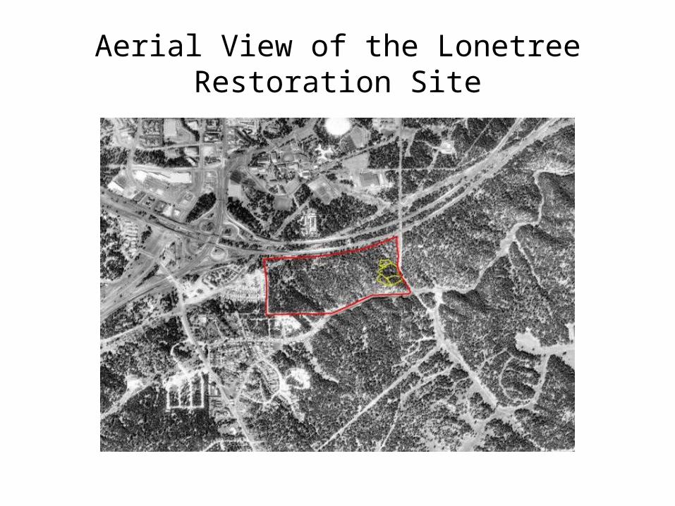
Aerial View of the Lonetree Restoration Site

Treatment Areas
Treatment Units
Project Boundary
Plots

Methods
Project layout• Boundaries and plot centers were plotted using a
Tremble Geoexplorer 2 GPS unit • GPS data was and differentially corrected using USDA
FS base station data from Cedar City, Utah and brought into an ESRI Arcmap project
• Plots were created using center points and plot direction• Plot data was imported into Arcmap and linked to
corresponding features • Pre- and post-treatment photos were hyperlinked to the
point location they were taken• Features were overlaid on an aerial photo and topo map


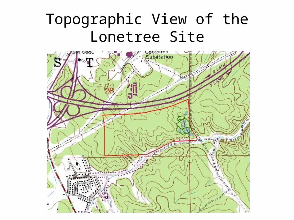
Topographic View of the Lonetree Site

Methods (Continued)
Tree Data• Trees were plotted in Arcmap using x-y data collected on
site and corresponding data attached to each tree• Crown diameter was estimated using allometric
equations for ponderosa pine (McTague, 1988)• Crowns of trees were projected and canopy closure was
estimated• Tree density and basal area was calculated using plot
data

Formulas for Estimate Canopy from DBH
• When D > 20 in:CST= (131.58 D - 1578.95) / {43.85exp (-333.54 / SD.99697))
+.012729 SD1.175 + 4.5}
S = Site Index (60)
D = Diameter in inches
• When D < 4 in:CY = .426 + 1.317 D
• When 4 < D > 20:C = (D – 4.0)[(CST, D=20) – 5.7] / 16.0 + 5.7
(McTague, 1988)
CST=Crown Diameter of Saw timber
CY=Crown Diameter of young trees

Assumptions
• Area of each plot was slope corrected for estimating tree density and basal area
• Pre-settlement date used was 1870 (approximate time of fire exclusion)
• Tree densities– Pre-settlement – assumed pole density by including living pre-
settlement trees in total tree density calculation
• Basal areas– Pre-settlement were calculated using the DSH of remnant stumps
– Living pre-settlement trees and pole basal area not included
• Crown closure– Canopy only estimated within plot using allometric equations
– does not include canopy extending beyond plot boundaries or the canopy of trees rooted outside plot
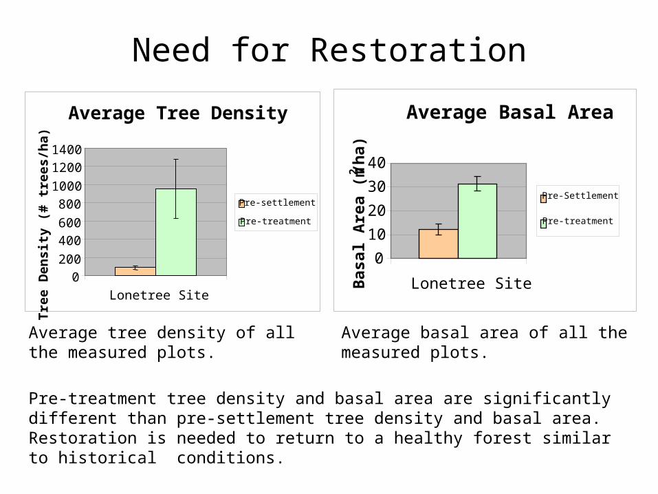
Need for Restoration
Average tree density of all the measured plots.
Average basal area of all the measured plots.
Pre-treatment tree density and basal area are significantly different than pre-settlement tree density and basal area. Restoration is needed to return to a healthy forest similar to historical conditions.
Average Basal Area
0
10
20
30
40
Lonetree SiteBas
al A
rea
(m2 /h
a)
Pre-Settlement
Pre-treatment
Average Tree Density
0200
400600
800
1000
12001400
Lonetree SiteTre
e D
ensi
ty (
# tr
ees/
ha)
Pre-settlement
Pre-treatment

Need for Restoration (cont.)
Pre-settlement Diameter Distribution
0
5
10
15
20
25
10 20 30 40 50 60 70 80
DBH (cm)
Tree
s/he
ctar
e
Diameter Distribution of 2000 Plots
0
200
400
600
800
1000
1200
10 20 30 40 50 60 70 80
DBH (cm)
Tree
s/he
ctar
e
Pre-settlement trees show a normal distribution around 40-50 cm DBH. The pre-treatment trees show a logarithmic (reverse J) distribution.

Lonetree Restoration Project Plots

NAU-99-2Pre-settlement, Pre and Post-treatment Canopy Covers
NAU-99-2 Tree Densities
050
100150
200250
300350
400450
NAU-99-2
Tre
e D
ensi
ty (
# tr
ees/
ha)
Pre-settlement
Pre-treatment
Post-treatment
NAU-99-2 Basal Areas
0
5
10
15
20
25
30
35
40
NAU-99-2
Bas
al A
rea
(m2/h
a)
Pre-settlement
Pre-treatment
Post-treatment
NAU-99-2 Crown Closure
0.0%10.0%20.0%30.0%40.0%50.0%60.0%70.0%80.0%90.0%
Plot NAU-99-2
Pre-settlement
Pre-treatment
Post-treatment

NAU-99-2: POST-TREATMENT PICTURES (P2)
August 21, 2000 November 9, 2004

NAU-00-2
Pre-settlement and Pre-treatment Canopy Covers
NAU-00-2 Tree Densities
0
500
1000
1500
2000
2500
3000
NAU-00-2
Tre
e D
ensi
ty (
# tr
ees/
ha)
Pre-settlement
Pre-treatment
NAU-00-2 Basal Areas
05
101520253035404550
NAU-00-2
Bas
al A
rea
(m2/h
a)
Pre-settlement
Pre-treatment
Crown Closure
0.0%
10.0%
20.0%
30.0%
40.0%
50.0%
60.0%
70.0%
80.0%
Plot NAU-00-2
Pre-settlement
Pre-treatment

NAU-00-2: PRE AND POST–TREATMENT PICTURES (0P)
Pre-treatment. September 6, 2000. Post-treatment. November 9, 2004.

Additional Analyses
• Location- find coordinates for any feature
• Measurements- distance, area, perimeter
• Spatial relationships- clumpiness, connectivity, proximity
• Patterns- data visualization
• Trends- changes in data over time
• Modeling- predict outcomes of different restoration alternatives

GIS to Visualize Restoration Prescriptions
10 m recruitment radius
Pre-settlement Evidence
Pre-settlement Live tree Post-settlement Live Trees

Comparing Restoration Prescriptions
Possible treatment using a 1.5 to 1 replacement for pre-settlement evidence
Possible treatment using a 3 to 1 replacement for pre-settlement evidence

Conclusion
• ALL project data (maps, photos, plot data) can be stored, organized and displayed in one GIS project
• Project data can utilize other GIS data for additional analysis
• Pre-settlement canopy closure and spatial distribution (i.e. “clumpiness”) can be reconstructed, analyzed and displayed
• Spatial analysis can aid in selecting replacement/ leave trees in restoration treatments
• Various prescriptions can be compared and visualized prior to implementation
• Future monitoring information can easily be incorporated and compared to previous data