by chaiwoot chaipan tien dung nguyen and mitsuo ezaki
TRANSCRIPT

Discussion Paper No.147
Regional Economic Integration and its Impacts on Growth, Poverty and Income Distribution:
The Case of Thailand *
by
Chaiwoot Chaipan1, Tien Dung Nguyen2 and Mitsuo Ezaki3
September 2006
* This research was financially supported by the Core University Program and the Grant-in-Aid for Scientific Research (B) of the Japan Society for the Promotion of Sciences (JSPS) in the fiscal year 2005. The socio-economic survey of Thailand was processed for the data base of our CGE modelling by Miss Sasipen Bhuvapanich (Ph.D. candidate, Graduate School of International Development, Nagoya University). We acknowledge them with appreciation.
1 Faculty of Economics, Chulalongkorn University, Thailand 2 Research and Development Center, National Advanced Training Institute, Ministry of Trade, Vietnam 3 Graduate School of International Development, Nagoya University, Japan
1

Abstract
Along with the regional frameworks, Thailand has made serious efforts to
establish Economic Partnership Agreements, including Free Trade Agreements (FTAs),
with several countries: China, India, Australia, New Zealand, Japan and the US. The aim
of this paper is to discuss a policy simulation analysis on the economic impacts on
Thailand’s economy of free trade agreements using a Global Computable General
Equilibrium (CGE) model. Suffice it to say that the FTA strategy and the formation of
Free Trade Areas in East Asia would stimulate growth and investment, and improve
welfare for Thailand. However, the impacts on income distribution vary with the
integration scenarios, depending on the pattern of production and trade and the extent of
trade liberalization in Thailand’s FTA partners. The simulation results show that Thailand
would gain most from the FTA with Japan both in terms of welfare and improved income
distribution; and that Thailand could realize most of the potential gain from free trade by
promoting the process of regional economic integration in East Asia.
Table of Contents
1. Pattern of Thailand’s Trade Policy
2. A Thailand-Japan FTA
3. Regional Integration in East Asia
4. Situation of Poverty and Income Distribution
5. Model Specification
6. Simulation Analysis
7. Concluding Remarks
References
Appendix A: Regional and Industrial Classification
Appendix B: The Global CGE Model
2

1. Introduction Regional integration has become a coexistence with the principle of multilateral
trade in the process of globalization of the world economy. According to a recent report
published by WTO, more than 259 regional trade agreements are in place (WTO
secretariat, 2003). Since the European Union (EU) and the North America Free Trade
Agreement (NAFTA) significantly had the effect of promoting intra-regional trade, other
countries have become active to explore options for such regional agreements.
In Asia, such trend has recently come to surface. The ASEAN Free Trade Area
(AFTA) has become effective since 2003. The Japan-Singapore Economic Agreement for
a New Age Partnership was concluded and took effect in 2002. China and ASEAN also
concluded a framework agreement toward the establishment of their free trade agreement.
Along with these regional frameworks, Thailand has made serious efforts to
conclude Economic Partnership Agreements (EPAs), including Free Trade Agreements
(FTAs) with several countries. In particular, it has concluded the agreements with China,
India, Australia, New Zealand, and most recently Japan. Now, it is negotiating with the
US.
It should be noted that most of the FTAs between Thailand and its partners cover
not only liberalization of trade, but also various types of economic cooperation. Some of
them are termed as Closer Economic Partnership Agreement (Thailand-Japan, Thailand-
Australia) or Trade and Investment Framework Agreement (Thailand-US). The main
elements of these new types of FTAs involve bilateral liberalization and facilitation of
trade through reduction of tariff and non-tariff barriers as well as the mutual recognition
of national standards, streamlining customs procedures, facilitation of increased services
trade and establishment of a framework for foreign investment. They also enhance
collaboration on intellectual property, education and tourism. In some extent, the basic
philosophy of these new types of FTAs is similar to that of Asia Pacific Economic
Cooperation (APEC) forum.
Theoretically, when an FTA is used as a market integration mechanism, it will
bring about tangible economic benefits when trade creation exceeds trade diversion effect.
The total economic effects are likely to be positive due to market expansion and cost
reduction. However, opponents of FTAs may raise strong criticisms that the agreements
3

are not sufficient for growth. Thailand, for example, also needs other supportive policies.
The protection of infant industries against imports will provide an opportunity of learning
and growing up. The openness of the country has been accompanied also by concerns
that it will cause some negative impacts, and that the poverty incidence and distribution
of income in Thailand will deteriorate. Accordingly, the issue of trade liberalization and
poverty in Thailand has become the focus of much research in the last several years.
The argument is also based on the truth that the potential advantages gained
from an FTA will vary in accordance with the counterpart’s economic structure and trade
patterns. Moreover, integration of the domestic market with that of another country will
create winners and losers for both parties. In this context, political consideration must be
paid to alleviating and minimizing the internal discord that may stem from external
integration.
It is obvious that Japan, China, India, Australia and New Zealand have regarded
FTAs as a fundamental element of their external economic policy. In this context,
Thailand would be an ideal FTA partner for them for several reasons. First, an agreement
with Thailand should be manageable since Thailand’s economic scale is much smaller
than that of those countries. Moreover, Thailand’s proximity (distance, size and area) is
seen as a positive factor that could yield geographical benefits, in term of regional
integration. Second, since Thailand’s average tariff rate of 17.4 percent is still above the
world level of 7 percent, the potential benefits for Thailand and its partners, related to an
elimination of tariffs, would be considerably higher than that for other nations. Finally,
the Thai government is still confident of pursuing FTA negotiations with other countries.
With strong political power, the Thaksin administration has the potential to find ways to
mitigate the negative impacts and emerging political conflicts.
The aim of this paper is to discuss a policy simulation analysis on the economic
impact of FTAs and regional integration in East Asia applying Computable General
Equilibrium (CGE) model. The simulation experiments of the Global Linked CGE model
developed by Nguyen and Ezaki (2005) are to analyze the impact of FTAs between
Thailand and its trading partners on the Thai economy with special reference to China,
India, Australia, New Zealand, Japan and the US. The conclusion drawn from these
4

model simulations will help to clarify the main source of an economic impact of FTAs
on growth, poverty and income distribution.
The paper is organized as follows. In sections 2 and 3, the descriptive analysis is
provided to understand the background and political pressure behind the Thai trade policy,
particularly a Thailand-Japan FTA. This will be followed by the development of regional
integration in East Asia and the situation of poverty and income distribution in Thailand
prior to the FTA policy in sections 4 and 5. An analytical framework of the CGE model
used for the simulation experiments is then presented in section 6. The outcomes of the
policy simulations are discussed in section 7. Finally, the paper will provide readers with
concluding remarks and some policy options.
2. Pattern of Thailand’s Trade Policy Obviously, one of the main reasons of Thailand’s free trade agreements is to
make the country more attractive place for foreign investment. The FTAs provide
investors with competitive advantages in the importation of raw materials, components
and other production inputs. They also open new markets and industries to local and
foreign direct investment, such as the ASEAN Investment Area (AIA) Agreement and the
Thailand-Australia FTA, which enables Australian investors to own majority control of
investments in selected industries in Thailand. Some FTAs harmonize customs codes and
product standards to speed up trade flows that will increase Thailand’s allure as a
production and export base.
The pattern of concluded FTAs can be described as follows:
ASEAN Free Trade Area (AFTA)
AFTA was launched in 1992 to eliminate tariffs and integrate member
economies into a single production base and regional market of about 550 million people.
Tariffs were reduced to 0-5 percent in 2003 for ASEAN-6 (Brunei, Indonesia, Malaysia,
the Philippines, Singapore and Thailand)and will be eliminated totally by 2015 for all
ASEAN members. Relatively, trade within all of ASEAN members is already free, as
more than 99 percent of traded goods are either duty free or face maximum tariffs of only
5 percent. In terms of liberalization of investment, the AIA agreement, a component of
5

AFTA, is supposed to facilitate member and non-member investors. Effective January 1,
2010, ASEAN-6 markets will be open to investors in most sectors, including
manufacturing, agriculture, fishery, forestry, mining and related services. Moreover, the
AIA will facilitate freer flows of capital, skilled labor, professional expertise and
technology within ASEAN.1
Thailand-China
Prior to the establishment of the ASEAN-China FTA, Thailand entered into an
FTA with China that took effect in October 2003. It eliminated duties on 188 fruits and
vegetables. But negotiations regarding additional items are on hold, as they will be
covered under the ASEAN-China agreement. China was the first important trading
partner selected by Thailand for forming an FTA. At first, China’s growing competitive
edge was regarded as a threat because it induced FDI away from Thailand and other
ASEAN countries. Such an attitude has changed since China joined the World Trade
Organization (WTO) in 2001. This is incorporated with China’s strategy of forming
FTAs with neighboring countries. In addition to the export market for Thailand, China
has offered various incentives such as an early harvest, or advanced trade liberalization,
in agricultural products. The highest growth rate of Thailand’s exports to China of about
60 percent is one of the main reasons direct to the point.
ASEAN-China
The ASEAN-China trade agreement on goods took effect on July 1, 2005,
creating the world’s largest free trade area of 1.7 billion consumers. Thai exports of
tapioca, biochemicals, plastics and medical equipment are expected to profit from the
FTA. Tariffs will be phased out between 2010 and 2018. But an Early Harvest Scheme
(EHS) between China and ASEAN-6, begun in January 2004, cut tariffs on meat, fish,
1 The study on the impacts of AFTA using GTAP model and CAMGEM of Chulalongkorn and Monash Universities found that trade liberalization within ASEAN would generate prosperity for the region as a whole. Singapore is likely to gain most from the implementation of AFTA policy. This benefit is gained from external impact caused by the tariff reduction on the part of other ASEAN members. In contrast, Thailand’ benefit would come mostly from the internal impact due to its own tariff reduction. See Arunsmith, Mallikamas, Treerat and Pornchaiwiseskul (2002).
6

dairy products, other animal products, trees, vegetables, fruits and nuts. Duties on these
goods are subject to be eliminated by 2006.
Thailand-India
An EHS, part of a broader Thailand-India FTA, took effect on September 1,
2004. The Scheme reduced tariffs on 82 agricultural and industrial items by 50 percent,
including various fruits, wheat, sardines, salmon, mackerel and processed crab. It also
covers other major Thai exports such as gems and jewelry, household electrical
appliances, integrated circuits, furniture and auto parts. Tariffs on these items will be
eliminated by September 1, 2006. Full liberalization will occur by 2010.
The main purpose of the Thailand-India FTA is to intensify trade and economic
cooperation between the two countries. Thailand and India share not only age-old bonds
of cultural affinity, commercial interests and common perceptions on various issues, but
also the possibility to increase trade and investment (Das, Ratanakomut and Mallikamas,
(2002)). In 2003, bilateral trade between the two countries was still at the low level, but
the growth rate of Thailand’s exports to India of about 54 percent was only second to
China. In addition, for Thailand, India is a gateway to the trading blocs in South Asia,
and promoting trade and cooperation with India can offset worries of China’s dominance
in the region. But for India, the deal is being viewed with concern for three reasons. First,
the Indian industry is not yet sure about its competitive efficiency. Second, many sectors
say they do not want competition on their homeland. And finally, there is a huge fear
among Indian companies that the deal will be misused as a staging ground for cheaper
exports to India. However, the deal can lead to an India-ASEAN FTA, and can bring
India closer to the region’s economic powers, such as Japan, China and South Korea.
Thailand-Australia
The Thailand-Australia FTA took effect on January 1, 2005. It eliminated
Australia’s 5 percent import tax on autos and parts. It also provided incentives to attract
Australian foreign direct investment. Australian investors can now own up to 60 percent
in Thai SMEs in telecommunications, computers, construction, education, distribution,
tourism, mining and other sectors. The FTA is expected to boost bilateral trade
7

significantly. Besides, the agreement eliminated tariffs on 83 percent of Thai exports and
80 percent of Australian exports, and by 2010, 95 percent of all trade between Australia
and Thailand will be free. Duties on all Thai agricultural products were eliminated,
except for tuna, skipjack and bonito, which will be phased out by 2007. Import duties on
Australian wheat barley, rye, oats, lactose, cocoa, copper bars and steel slab were
eliminated, while tariffs on items such as wine, fruits, vegetables, plastics, paper, textile,
garment, steel, machinery and electrical appliances will be eliminated by 2010.
Thailand-New Zealand
The Closer Economic Partnership Agreement between Thailand and New
Zealand took effect on July 1, 2005, eliminating duties on 71 percent of annually traded
goods. Tariff-free imports from New Zealand include machinery, wool, plastic products,
paper, infant formula and vegetables. Thai exports, including electrical appliances, gems,
canned tuna, furniture, glass and ceramics, are tariff-free.
The main objective of setting up the FTAs between Thailand and Australia and
New Zealand is to enhance trade and improve welfare. Although trade between Thailand
and the two countries is still playing small part in improving Thailand’s welfare, better
trade and crisis management are seen to be a main ingredient to promote trade and
growth in Thailand. Since Australia and New Zealand are known to be more advanced
and competitive in the technology and management sector, a good trade policy and
economic cooperation will enhance Thailand’s welfare.
3. Thailand-Japan FTA In July 2005, Thailand and Japan reached basic agreement to sign a free trade
agreement. Officials from the two sides have shown their hard works since the
negotiations began in February 2004. Despite a lot of conflicts of interests, they have
managed to conclude the negotiations in an uneventful manner. Upon close scrutiny of
the working-level negotiations between the two governments and the consequences of
FTA mainly with China, it seems that the Thai government has displayed competent
negotiating skills.
8

Discussions of a Thailand-Japan FTA began with a Thai proposal in November
2001 that Thailand and Japan should explore together the possibility of establishing a
bilateral Free Trade Agreement. In January 2002, Japan then proposed the “Initiative for
Japan-ASEAN Comprehensive Economic Partnership”. With these proposals serving as
an impetus, Thailand and Japan decided to begin consultations for an agreement of Japan-
Thailand Economic Partnership (JTEP) in April 2002. The working group was
subsequently set up that resulted in the publication of a task force report in December
2003, which presented a positive assessment of the potential for JTEP agreement.
Under the agreement, Thailand is subject to lower its import duties on cars with
an engine of 3000 cc or larger from the present 80 percent to 60 percent by 2010. Import
duties on auto parts will be phased out entirely by 2011, and those on steel products will
be eliminated within 10 years of the implementation of the agreement. As for Japan’s
concessions, rice is to be exempted, while import duties on pork are to be lowered from
21.3 percent to 10.65 percent in five years after the agreement goes into effect and a low
import-duty framework will be set for bananas. Thai care workers will be permitted to
enter into Japan, while the length of previous work experience as a precondition for Thai
cooks residence in Japan will be shortened from the present 10 years to 5 years.2
The Thailand-Japan FTA would enhance intra-industry trade, while trade and
investment between the two countries would expand as a result of elimination of tariff
and non-tariff barriers. This would contribute to economy of scale advantages and
enhanced production efficiency. Furthermore, the FTA would involve such positive
2 The quantitative effects of trade liberalization between Thailand and Japan were shown in the appendix of
the task force report in December 2003. Taking into account the dynamic impacts such that through capital
formation mechanism, one by the accumulation of induced income, savings and investment, and another by
international capital movements and through pro-competitive productivity growth effects, the
macroeconomic gains from trade liberalization is estimated to be larger than the static impacts. Japanese
real GDP would increase by 0.24 percent. In contrast, real GDP in Thailand would increase by 20.09
percent. Macroeconomic gains measured in terms of rate of changes are much more significant in Thailand.
Welfare improvements measured by Equivalent Variation (EV) are estimated to be around US$ 13 billion
in Japan, while US$ 23 billion in Thailand. Moreover, the benefits of trade liberalization could be higher
for this region if Thailand-Japan FTA leads to Japan-ASEAN FTA and further global trade liberalization.
9

economic effects as an expansion of foreign direct investment (FDI) through promotion
of the standardization of advanced technologies, development of human resources and
establishment of a more transparent and sound investment environment. The importance
of the Thailand-Japan FTA can be recognized that it is hailed by the Thaksin
administration as one of its major achievements in the conducts of its international
economic policy.
However, there have been those who have adopted a more negative view of the
FTA, due to concerns that the actual benefits received by Thai traders will depend in
large part on how much access is actually gained to the Japanese market, and that the
Thai industrial and business sectors cannot effectively improve their competitiveness.
Very little information has been made public by the Thaksin government, despite
persistent calls for transparency from civic groups and business operators concerned
about the negative impact of the FTA. The government has not tabled the matter for
debate in the House of Representatives, claiming that the FTA is not a treaty. Previous
FTAs signed between Thailand and its partners, particularly China, have adversely
affected a large number of Thai farmers and small business operators, while the business
elite benefited handsomely. In the case of Japan, the effects on Thai farmers and small
business operators will be greater because the FTA covers diverse areas of trade and
investment.
In Japan, most newspaper commentaries also echoed the criticism of the
agreement with Thailand, calling it far short of what a free trade agreement should
achieve. Along with these comments, it was criticism of the Japanese government for
failing to take an initiative in opening Japan’s own market as a major trading power that
should play role of promoter of the principal of free trade.3
4. Regional Integration in East Asia The shift towards regional integration in East Asia during the last decade might
be rooted in the financial crisis started in Thailand in July 1997. The cooperation in
particular among the ASEAN+3 (ASEAN, Japan, South Korea and China) has been
proceeding firstly on financial issues. Urata (2004) explained that based on this platform 3 See Foreign Press Center Japan, August 15, 2005.
10
East Asia will develop to become a Free Trade Area for three reasons. First, the Doha
Round has encountered difficulties to promote freer trade on a global scale. Second, East
Asian economies have become interested in using FTAs as a way of promoting
deregulation and structural reforms in the domestic market. And third, the lack of
adequate international assistance during the recent economic crisis illustrated the need for
solidarity between the countries of the region.
During the recent economic crisis, it was argued that Japan was more
complementary than competitive to the rest of Asia, and potentially could benefit greatly
from a free trade area in East Asia. Moreover, Japan was the sole developed country in
the region, and should become a major impetus to regional integration (Lau (2003)). In
January 2002, Japan then signed the Japan-Singapore Economic Partnership Agreement
(JSEPA), indicating the shift of the Japanese policy on FTA. Japan’s position is that to
establish an East Asia free-trade Zone in 2010 (Japan Times (2002)). It would encompass
Japan, ASEAN, China, South Korea and Taiwan or the so-called ASEAN+5. In the future,
the area could be extended to Australia and New Zealand, as well as the US. The aim is
to offset the economic challenges posed by the European Union and the North American
Free Trade Agreement Zone. It would also overcome the difficulties that the World Trade
Organization has encountered in trying to promote freer trade on a global scale.
China also proposed the trade area in 2003. Since joining the WTO in 2001,
China has not only secured access to the world market, it has also started to develop
regional trade. It signed the China-Hong Kong Economic Partnership Agreement (CEPA)
in June 2003. But the plan to establish an ASEAN+3 trade zone made no progress, China
then decided to negotiate with ASEAN and concluded the FTA in 2005. From China’s
point of view, Korea and Japan would follow the same strategy, exploring the possibility
of similar negotiations with ASEAN.
In the case of ASEAN, it prefers to deal with the partner countries on separate
basis. Its strategy is to become a hub. It has negotiated and signed FTAs with many
countries inside and outside the region such as Japan, China, the US, the EU, India,
Australia and New Zealand. This strategy of ASEAN has created fears for some of its
members that foreign companies would use Singapore as an assembly site or distribution
center from which their products would be exported to other member countries duty free.
11

As mentioned before, Thailand has also set its position to deal with partner
countries on separate basis. But it supports the establishment of an East Asia Study
Group (EASG) to explore practical ways to expand existing cooperation and to form new
linkages in all sectors. From Thailand’s point of view, the ASEAN+3 integration process
would focus its activities on narrowing the development gap within ASEAN and between
ASEAN and East Asia.4
There are several approaches that could help establish an East Asia Free Trade
Zone. But Lu (2003) saw that the most possible path would take two stages of process.
The initial stage is to establish various FTAs among pairs and groups of regional
economies. Then the final stage is to merge individual FTAs into a region-wide
framework. From this point of view, the first stage has already well started.
5. Situation of Poverty and Income Distribution Generally, it can be said that FTA has the potential to act as a significant catalyst
for poverty reduction. It can provide poor people in the partner countries with access to
the market, technologies, and ideas needed to sustain higher and more equitable patterns
of growth. However, to understand it clearly, one has to recognize that growth is a
necessary, but not a sufficient condition, for a sustained reduction in poverty reduction.
Even if trade liberalization is linked to more rapid growth, this does not necessarily imply
that it is an effective instrument for reducing poverty. For instance, if a growth strategy
based on the reduction of trade restrictions leads to a considerable decline in income of
households at the bottom of the income strata, it may not make any inroad in alleviating
poverty. The effectiveness of FTA measures then depends on the linkage between trade
liberalization and income distribution.
The World Bank (2001a and 2001b) recognizes that there may not be a direct
link between trade policy measures and income distribution. The Kuznets curve
hypothesis, which claims to be the existence of a U-shaped link between growth and
inequality due to the shift from the agricultural to the nonagricultural sectors, seems not
to be empirically valid in many cases. It still depends on appropriate macroeconomic and
exchange rate policies. In other words, to be successful, trade reforms must be part of a 4 Ministry of Foreign Affairs of Thailand, July 8, 2003.
12

logically consistent package of sound macroeconomic and exchange rate policies and
structural reforms.
The last point to be concerned about is the link between FTAs and rural and
agricultural sector. Take Thailand for instance, while it has seen a significant increase in
the share of manufactures in their exports after trade liberalization, a large proportion of
the population is still closely tied to the rural sector and in agriculture. This sector is
where the bulk of the poverty is concentrated (Chaipan and Grosskopf (1995)).
To quantify the effect of trade agreements on poverty and income distribution in
Thailand, it is worth to mention the situation prior to the policy measures. The latest data
complied by National Statistical Office of Thailand and Office of the National Economic
and Social Development Board indicated that Thailand is the land of inequality. In 2004,
the Gini coefficient was 0.408, among the highest in Asia. The richest 20 percent of the
population in this country earned 48.6 percent, while the poorest 20 percent earned only
6.1 percent of total income in that year. Moreover, while Thailand can reach the more
developed country status, income inequality in this country has increased significantly
since the 1960s (Ikemoto (1991), Ikemoto and Uehara (2000)). Although during the last
two decades, Thailand’s poverty incidence was decreased from 32.5 percent in 1992 to
12.0 percent in 2004, mainly due to its economic growth, the increase in inequality could
still be problematic from the perspective that it might slow the GDP growth rate in the
years to come. The inequality has been found particular significance in the agricultural
sector for two reasons. First, while the share of the agricultural sector in GDP decreased
from 27 percent in 1974 to 10 percent in 2003, the labor force in this sector in 2003/2004
still accounted for 42 percent of the total labor force. Second, income level in agricultural
sector was low and volatile because farm prices and harvest directly affect the value of
agricultural output. For many authors, this characteristic of the Thai economy leads to the
conclusion that the Kuznets Hypothesis is the most importance for understanding changes
in Thailand income distribution.
Moreover, Thailand has also faced the interregional inequality. The average
household income in the Bangkok Metropolitan area was 2.6 times higher than that of the
rural area in the Northeast region in 1975-76. The figure had increased to 3.4 in 1998 and
4.5 in 2001. Motonishi (2003) found that total inequality in Thailand increased in the
13

1980s, and was relatively stable in the 1990s. But interregional inequality increased in the
late 1980s till the early 1990s, and decreased afterward. The main determining factor of
inequality in Thailand is the inequality between the agricultural and nonagricultural
sectors. The other determinants, including financial development, education level
disparity and aging, are not significantly responsible for the increase in inequality in
Thailand.
6. The Model Specification The global CGE model employed in this paper is an extension of the global
model developed by Nguyen and Ezaki (2005) to analyze the impacts of regional
integration on Vietnam’s economy. We extended the model by Nguyen and Ezaki (2005)
basically in line with GTAP world model (Hertel (1997)) to allow for a greater regional
and industrial disaggregation, a detailed treatment of taxes and subsidies, international
capital mobility and transportation costs. The current global CGE model specifies 20
industries and 16 regions. The regional classification is focussed on East Asia, consisting
of all major economies in the region as well as the US, the EU and Oceania. Industrial
activities are specified with an emphasis on the agricultural and manufacturing sectors,
taking into consideration the diversified pattern of production and comparative advantage
as well as the structure of protection in each individual country and region. The details of
the regional and industrial classification are given in appendix A.
Country models
The global CGE model consists of 16 country models, which are linked together
through international trade and foreign investment. Country models generally follow the
standard neoclassical CGE model (Dervis et al. (1982)), in which capital and labor are mobile
across economic sectors with the assumption of full employment. For each country model, there
are three production factors, i.e. capital, skilled labor and unskilled labor. Skilled and unskilled
labor are combined in a Constant Elasticity of Substitution (CES) function to form a
composite labor input, and sectoral output is a CES function of capital and composite
labor.
14

In each country model, nine kinds of taxes and subsidies were specified,
consisting of tariffs, export duties, production taxes, capital and output subsidies, and
sales taxes imposed on consumer goods, intermediate inputs and capital goods. The
detailed treatment of taxes and subsidies makes it possible to analyze other policy
instruments in addition to tariffs. Government revenue consists of revenues from all taxes
and subsidies. Total government revenue is allocated to savings and consumption in fixed
proportions. The government demand for final goods is defined using fixed expenditure
shares of government real spending.
Household income consists of labor and capital income. To allow for a detailed
inspection of the impact of trade liberalization on income distribution in Thailand, the
household sector in Thailand’s model is disaggregated into 20 household groups
according to the level of income, consisting of 10 urban groups and 10 rural groups. On
the demand side, household consumption demand is determined using the Linear
Expenditure System (LES) function. The major advantage of the LES function is that it
allows for the effect of the change in income on the structure of consumption. As income
rises, people tend to spend less on agricultural goods and other necessities, and consume
more manufacturing goods.
The external sector in country models is modeled with the assumption of product
differentiation, in which domestic and foreign goods are imperfect substitutes. Sectoral
output is a Constant Elasticity of Transformation (CET) function of exports and
domestically produced products. The supply for domestic and foreign markets is
determined from the revenue maximization condition, depending on the relative prices at
home and abroad. Total domestic demand is satisfied through domestic production and
imports, and the demand for imports and domestically produced goods is modeled using
the Armington structure. In this treatment, the demand for imports and domestic products
varies with the changes in the relative prices of domestic products and imports.
International Linkages
Country models are linked together through trade and investment flows.
Domestic consumers and producers differentiate imports by sources, that is, imports
coming from different countries are considered as imperfect substitutes. This
15

characteristic is also modeled with the Armington structure. At the aggregate level, total
imports is a CES function of imports from different sources, and then the demand for
imports from each sources is derived from the cost minimization condition. On the export
side, exporters do not differentiate exports by countries of destination, that is,
commodities supplied to foreign countries are seen as perfectly homogenous and are sold
at the same price. The trade consistency is held so that total exports supplied by home
countries are equal to the sum of imports by foreign countries. To put it more specifically,
imports from a country or region must be summed up to total exports by that country or
region.
International transportation services create a wedge between the f.o.b prices in
exporting countries and the c.i.f. prices in importing countries. The transportation cost is
determined from the value of exports at f.o.b prices. The global demand for transportation
services is computed by summing across all countries and industries. The demand for
transportation services is then determined for countries and regions from the cost
minimization condition based on the CES functional form. Thus the regional demand for
transportation services will depend on the regional prices of transportation services,
which are converted into a global currency unit using the corresponding exchange rates.
The complementarity between trade and investment has been the subject in
many empirical studies. Trade liberalization changes the relative prices of production
factors, thereby affecting foreign capital inflows. Indeed, several studies have indicated
that the change in capital inflows resulting from trade liberalization could produce
considerable additional welfare gains. The link between trade and investment has been
accounted for in some recent studies using CGE models, such as those by Lee and
Mensbrugghe (2001) or Bchir et al. (2002). In these studies, investment or capital stock is
allocated across regions and industries, depending on the rate of return to capital.
However, both these approaches require detailed information on foreign investment and
capital at the sectoral level, which is not available at the level of the industrial and
regional disaggregation adopted in this paper.
In our model, we employed a somewhat simple approach discussed in Hertel
(1997) to allow for international capital mobility. In this approach, the expected return on
capital is assumed to decline with the addition to the capital stock at the rate determined
16

by a flexibility parameter. Investment decisions are made in such a way that the rates of
return on capital are equalized across countries and regions. Thus the change in global
savings is allocated across country and regions to equalize the regional expected rates of
return. In this treatment, investment only partially adjusts in response to the changes in
the rate of return caused by trade liberalization. At a low value of the flexibility
parameter, the expected rate of return to capital is not very sensitive to the change in
capital stock, thus a large change in investment is required to equalize the expected rate
of return to capital. A low flexibility parameter means a greater capital mobility and vice
versa.
Equilibrium Conditions
Equilibrium conditions consist of the conditions in factor, commodity and
foreign exchange markets. In the factor market, we adopted the assumption of full
employment, and factor prices serve as equilibrating variables. In the labor market, total
supply of skilled and unskilled labor is held fixed at the base-run level, and the labor
market equilibrium determines wage rates. Capital rents adjust to maintain the
equilibrium between the supply of and demand for capital in the capital market.
Equilibrium in product markets equates the supply of domestic goods in each sector to
the demand for domestically produced products, with domestic prices serving as
equilibrating variables.
The fiscal balance is implied in the treatment of the government sector, in which
government consumption and savings are determined as fixed shares of government
revenue. In the foreign exchange market, the exchange rates are fixed for all countries
and regions, and foreign savings are assumed to adjust to the change in demand for and
supply of the foreign exchanges. Savings and invest are determined independently in
each country or region but the savings-investment identity is guaranteed automatically by
the local Walras’ Law. We do not introduce the general price equation for each country
or region to control its price level except for the United States, in which the general price
level is fixed as the world numeraire by allowing for the global Walras’ Law. All the
exchange rates are fixed but the real exchange rates change because of the flexible
domestic price levels relative to the world numeraire.
17

7. Simulation Analysis Data and the Model calibration
To run the model, we made use of GTAP database version 6.0 constructed for
2001. 5 57 industries and 87 regions originally specified in GTAP database are
aggregated into 20 industries and 16 countries or regions in accordance with the model.
We used GTAP data to calculate most of the parameters in the model, such as
consumption shares, saving rates, tax rates, wage rates and capital rents. The elasticities
of substitution in trade and production functions are taken from GTAP database,
consisting of the elasticity of substitution between labour and capital, the elasticity of
substitution between domestically produced goods and imports and the elasticity of
substitution between imports from different sources. GTAP database gives high values to
the elasticities in trade functions, while assigning relatively low values to the elasticity of
substitution in production functions. We assigned a value of 1.2 to the elasticity of
transformation in the export supply function for all industries. Given the type of functions
and the value of the elasticities, the scale and share parameters can be calculated directly
from the benchmark data.
In Thailand’s model, household data is constructed using the socio-economic
survey conducted by the National Statistical Office of Thailand in 2000.6 The survey data
are grouped into urban and rural households, and each group is further divided into
deciles according to income ranges. Municipal areas are classified as urban areas, while
sanitary districts and villages are classified as rural areas in a broad sense. Types of
enterprise in which households belong to, together with the occupation of household
heads are used to define the sectors of households. Skilled labor and unskilled labor are
separated by level of education. Those with education attainment less than third-year
elementary (grade ninth) are categorized as unskilled labor. Consequently, income of
each labor type in twenty industries is obtained through total monthly income of
members of households aged equal or over 15 years old using criteria explained above to
5 More details about GTAP database version 6 can be found in GTAP homepage
(http://www.gtap.agecon.purdue.edu/). 6 The socio-economic survey is conducted every two years of even numbers. The survey of 2001 is exceptionally available for 2001 but only for a half of the year, so that the survey of 2000 is used in the model.
18

classify. Labor income is defined as wages and salaries, whereas capital income is profit
from non-farm business. Profit from farming is divided equally into labor and capital
income. Consumption data is based on household consumption expenditure on goods and
services provided in the survey.
The survey data is then incorporated into GTAP data using a relatively simple
procedure. Income shares are computed from the survey data, and are used to allocate the
data on factor income taken from GTAP database to each household groups and
industries. Similarly, the expenditure shares are computed, and are used to allocate GTAP
data on private consumption to household groups. Data on household employment is also
derived from the socio-economic survey 2000. This data is computed for each type of
workers, i.e. skilled and unskilled workers, and is used to allocate employment data
derived from GTAP database to household groups.
Simulation scenarios
We employed the CGE model described in the previous section to analyze the
impacts of regional economic integration on Thailand’s economy. Eleven simulation
scenarios have been performed and are described briefly in table 1. These simulations are
designed to cover all the major integration options currently facing Thailand, including
the bilateral FTAs between Thailand and China, Japan, India, Oceania and the US. In
addition, we also included in the simulation analysis the ASEAN free trade area (AFTA)
and the possible formation of the East Asian free trade area.
Table 1: Simulation Scenarios
S0 S1 S2 S3a S3b S4a S4b S5 S6a S6b S7a S7b
Base run ASEAN FTA Thailand-China FTA Thailand-Japan FTA, removal of tariffs Thailand-Japan FTA, removal of tariffs and agricultural subsidies Thailand –US FTA, removal of tariffs Thailand –US FTA, removal of tariffs and agricultural subsidies Thailand-India FTA Thailand-Oceania FTA, removal of tariffs Thailand-Oceania FTA, removal of tariffs and agricultural subsidies East Asian FTA, removal of tariffs East Asian FTA, removal of tariffs and agricultural subsidies
19

In both developing and industrial countries, domestic industries have been
protected not only by tariffs, but also non-tariff barriers and domestic subsidies. In many
cases, it is not tariffs but non-tariff barriers and subsidies that play a major role in
protecting domestic industries. The current version of GTAP database provides detailed
information on the tariffs and certain production subsidies in the form of output and
capital subsidies. However, it does not quantify the tariff-equivalent effect of non-tariff
barriers. Thus our simulation analysis focused mainly on the removal of tariff barriers
and quantified its impacts on Thailand’s economy. In addition to the tariff removal,
agricultural subsidies were also taken into account when they are found significant in
GTAP database. For the FTAs with developed countries like Japan, the US, Oceania
countries and the East Asian free trade area, two sets of simulations are performed. The
first set takes into account only the impacts of the tariff removal, while the second one
quantifies the combined effect of removing both tariffs and agricultural subsidies.
Macroeconomic Impacts of Economic Integration
The simulation results show that Thailand would gain significantly in terms of
output and welfare in all the FTAs in consideration. The magnitude of the gains, however,
is different, varying with the Thailand’s FTA partners. In the CGE model employed in
this paper, we can specify several sources for the gains in welfare and output. The first
source of the welfare gain is the level of protection prior to trade liberalization in
Thailand. Tariff reductions in Thailand reduce the prices of imported goods and improve
efficiency of resource allocation. The second source of welfare gains is trade
liberalization in Thailand’s trading partners. The removal of tariffs in trading partners
would expand the market for Thailand’s exports, thus stimulating the development of the
industries in which Thailand possesses a comparative advantage. Thus the gain from
FTAs depends on the geographical composition of Thailand’s trade as well as the level
and structure of protection in Thailand and its trading partners.. An FTA with a larger
trading partner would have a greater impact and bring about a greater welfare gain. The
third source of the welfare gain in this model comes from the linkage between trade and
investment. When trade liberalization is accompanied with an increase in investment, the
20

21
latter would further stimulate growth through its impacts both on the supply and demand
side.
The impact of AFTA on Thai economy was first investigated in simulation S1,
in which we removed the tariffs imposed on bilateral trade between Thailand and five
major ASEAN countries, namely Vietnam, Malaysia, Singapore, Philippines and
Indonesia. Combined together, these ASEAN economies occupy a large share in
Thailand’s trade, with Singapore and Malaysia being the largest trading partners in
Southeast Asia region. This indicates that trade liberalization in this region could bring
about significant gains for Thailand. As shown in the simulation results, real GDP of
Thailand increases by 0.4%, while the welfare index increase by 2.3%. In addition to
Thailand, Vietnam, Malaysia and Singapore are also the big gainers from AFTA
liberalization.
One of the major motives lying behind economic integration in ASEAN is to
improve the competitiveness of ASEAN countries and make them a production hub
capable of competing with China and India in attracting foreign investment. It is
interesting to see in S1 that, AFTA would significantly improve the investment
environment in ASEAN countries, as reflected in the increase in the return to capital
across the region. Since the model allows for capital to partially adjust in response to the
difference in the rate of return to capital, foreign investment would flow in ASEAN
countries following AFTA liberalization. For Thailand, the increase in real investment
amounts to 8.7%, largely compensating for the decline in government consumption and
leading to an overall output gain.

22
Table 2: Macroeconomic Impacts of Economic Integration on Thailand (Percentage changes compared to the base-run)
S1 S2 S3a S3b S4a S4b S5 S6a S6b S7a S7b
GDP deflator -
0.08 1.95 1.98 2.03 0.61 0.88 0.27 -0.42 -0.41 2.24 2.30
Consumer price index -
0.43 1.08 0.72 0.75 -0.01 0.22 -0.03 -0.65 -0.64 0.61 0.63Wage rate of skilled labor 1.65 3.07 3.47 3.50 1.45 1.53 0.69 0.13 0.13 6.58 6.60Wage rate of unskilled labor 1.87 2.75 5.63 5.73 1.60 2.12 0.56 -0.13 -0.12 8.78 8.88Capital rent 1.41 2.64 3.68 3.73 1.22 1.44 0.55 0.00 0.00 6.44 6.49Real GDP 0.41 0.65 0.54 0.54 0.16 0.14 0.12 -0.01 -0.01 1.66 1.66Output 0.82 0.87 0.62 0.60 0.36 0.17 0.19 0.17 0.17 1.72 1.69Private consumption 2.32 1.90 4.33 4.37 1.56 1.65 0.65 0.64 0.63 7.80 7.84Government consumption
-9.63
-2.56
-13.98
-14.04 -4.81 -5.02 -1.51 -2.76 -2.75
-25.45
-25.50
Real investment 8.68 9.12 18.26 18.47 5.42 5.62 1.84 0.77 0.78 30.21 30.42Imports 5.92 5.57 7.94 7.95 2.83 2.49 1.43 1.23 1.23 16.64 16.63Exports 2.63 1.84 0.64 0.56 0.60 0.18 0.55 0.80 0.79 4.29 4.19Household income 1.90 3.09 4.89 4.96 1.56 1.84 0.64 0.01 0.02 8.32 8.39Labor income (skilled labor) 1.65 3.07 3.47 3.50 1.45 1.53 0.69 0.13 0.13 6.58 6.60Labor income (unskilled labor) 1.87 2.75 5.63 5.73 1.60 2.12 0.56 -0.13 -0.12 8.78 8.88Capital income 1.94 3.20 4.83 4.89 1.55 1.79 0.66 0.05 0.05 8.39 8.45
Government revenue -
8.91-
0.57-
11.67-
11.69 -3.96 -3.94 -1.15 -2.95 -2.94-
22.12-
22.14Welfare 2.32 1.90 4.31 4.35 1.55 1.65 0.65 0.64 0.63 7.75 7.79 Sources: Authors’ calculation

The trade relation between Thailand and China has been on a rapid rise in recent
years, and is expected to further increase in the future following the implementation of
Thailand-China FTA and China-ASEAN FTA. China currently accounts for 5.2 percent
of Thailand’s total imports and 6.1 percent of total exports. The FTA between Thailand
and China was examined in simulation S2, in which tariffs were removed for bilateral
trade between countries. The simulation results show that this FTA would bring benefits
to both Thailand and China. On a relative term, Thailand would gain 0.7 percent in real
GDP and 1.9 percent in welfare. The FTA with China also increases foreign investment,
exports and imports in Thailand. However, the gain for China is only marginally given
the large size of its economy. . .
Unlike China, Japan has traditionally been the largest trading partner and foreign
investor in Thailand, and thus the FTA with Japan plays a very important role in
Thailand’s integration strategy. The FTA with Japan could not only brings about a greater
market for Thailand’s exports, but also luring Japanese FDI into Thailand and expanding
opportunities for other economic and technical cooperation. The impact on Thai economy
of the FTA with Japan was analyzed in simulations S3a and S3b. The first one only takes
into account the impact of the tariff removal, whereas the second one analyzes the
combined effect resulting from the removal of both tariffs and Japanese agricultural
subsidies.
The FTA with Japan would substantially increase the gain for Thailand as
compared to those with China and ASEAN countries. For Thailand, real GDP increases
by 0.5 percent, but the increase in welfare amounts to 4.3%, which is around two times
higher than the gain resulting from Thailand-China FTA. The increase in real investment
is also impressive, amounting to nearly 20 percent. The big welfare gain from Thailand-
Japan FTA not only results from the large trade volume, but also from the fact that the
two economies are more complementary than competitive. It should be noted that the
inclusion of Japanese agricultural subsidies in S3b does not significantly raise the welfare
gain for Thailand, even it may have some significant effect at the sectoral level as
discussed later.
While Japan is the largest import market of Thailand, the US is the largest
market for Thailand’s exports. As shown in simulations S4a and S4b, the FTA with the
23

US could bring benefits to Thailand, but to a lesser extent compared to the FTAs with
East Asian countries. Real GDP rises by only 0.2%, and the increase in welfare amounts
to 1.6%. Investment, exports and imports also increase less as compared to the previous
simulations. The removal of agricultural subsidies in S4b does not significantly affect the
results at the aggregate level. The relatively small gain from the FTA with the US is
largely due to the low level of protection in the US. Indeed the US market has been
largely liberalized for manufacturing products, while the US tariffs imposed on processed
food, textile and leather are well below the level adopted in Japan, China or ASEAN
countries.
The next three simulations examine the impacts of the FTAs with India, New
Zealand and Australia. All these countries, however, are not the major trading partners of
Thailand, accounting for only some percents of Thailand’s trade. The simulation results
show very modest gains from these FTAs. Real GDP of Thailand even declines slightly
in the case of Thailand-Oceania FTA, and this decline is largely due to the contraction in
agricultural production and food processing industries.
In the recent years, there has been an increasing interest in the establishment of a
free trade area in East Asia. The last two simulations (S7a and S7b) were designed to
examine the impact of the possible formation of the East Asian free trade area. This
simulation scenario takes into account all major economies in the region, consisting of
Vietnam, Indonesia, Malaysia, Philippines, Thailand, Singapore, China, Korea, Hong
kong, Taiwan and Japan. The first simulation (S7a) only investigates the removal of
tariffs, while the second one takes into account the removal of agricultural subsidies in
Japan and Korea together with the tariff removal. As shown in table 2, Thailand, together
with Malaysia, Korea and Vietnam, are the biggest gainers. For Thailand, GDP increase
by 1.7 percent in real terms, and the welfare index increases by 7.8 percent. Thailand also
gains a lot in terms of foreign capital inflows, with the increase in real investment
amounting to over 30%. Similar to the case of the FTA with Japan, the removal of
agricultural subsidies could bring about some additional benefits at the aggregate level,
but only to a marginal extent7.
7 The East Asian Free Trade Area has been investigated in some recent studies, including Urata and Kiyota (2003) and Kawasaki (2003). These studies have also reached conclusions similar to our analysis, showing
24

It is interesting to note that the welfare gain of Thailand is largely attributed to
trade liberalization in Japan. Thailand-Japan FTA contributes more than half of total
gains in welfare and investment under the East Asian free trade area. Among the bilateral
FTAs, Thailand gains most from the FTA with Japan, which is the largest trading partner
of Thailand. The simulation results also indicate that Thailand could gain more from the
FTAs with the trading partners in East Asia than those with the partners outside the
region. Furthermore Thailand could realize most of the potential gain from free trade by
promoting economic integration in East Asia.
.
Sectoral Impacts of Economic Integration
We continued the discussion in this section with an analysis of the impacts of the
FTAs at the sectoral level. The sectoral impacts of regional integration are largely
determined by the structure of trade and protection in Thailand and its trading partners.
The industries, which are highly protected prior to trade liberalization, are likely to
contract when tariffs are reduced. By contrast, the industries facing high protection in
foreign markets are expected to grow following the removal of trade barriers in foreign
markets. Since the trading partners involved in the investigated FTAs are very diversified
in the level of development, the pattern of comparative advantage and the resulting
structure of protection, these FTAs are likely to have different impacts on Thailand’s
production and trade at the sectoral level.
In regards to ASEAN, Thailand trades mainly in electronics, transportation
means and some other heavy industries. Although agricultural and labor-intensive
products are the major exports in many ASEAN members, Thailand’s trade with ASEAN
countries in these products is rather small. This reflects the fact that most ASEAN
members have a comparative advantage in agricultural and labor-intensive products, and
that these products are usually protected with high tariffs in Thailand’s domestic market.
For Thailand and more advanced ASEAN countries, AFTA trade liberalization leads to positive impacts on all East Asian economies. The welfare gains from our simulation analysis, however, are lower than those found in Urata and Kiyota (2003) and Kawasaki (2003). This is largely due to the differences in the database and model structure. Urata and Kiyota (2003) and Kawasaki (2003) employed GTAP database version 5.0, and thus are able to quantify the impacts of both tariffs and non-tariff barriers. Furthermore, the very high welfare gains found in Kawasaki (2003) are largely attributable to the productivity and capital accumulation effects incorporated in his model.
25

an expansion in trade and production in electronics, transportation means and some other
heavy industries, but a contraction in agriculture and labor-intensive industries. Vietnam
and less developed ASEAN members experience an expansion in the production of
agriculture and labor intensive industries, where they possess a comparative advantage.
For Thailand, the changes in the pattern of trade and production resulting from
Thailand-China FTA are generally similar to those under AFTA trade liberalization.
Output declines in agriculture, textile and leather, but expands in most heavy industries
with capital intensiveness. The changes in the production pattern occur in an opposite
direction in China, with a contraction in heavy manufactures and an expansion in
agriculture and light manufactures. For some industries like electronics and transportation
means, production expands in both countries largely due to the increase in intra-industry
trade. The similar changes in production and output are also observed in the case of
Thailand-India FTA, although the extent of changes is much smaller.
Unlike the FTAs discussed above, the other FTAs involve trading partners from
industrial countries like Japan, the US and Oceania. Since all these economies are more
complementary to Thailand in economic terms, forming FTA with them is expected to
have greater impacts on resource reallocation. In the FTA with Japan, agriculture and
food processing industries experience a big gain in output, and this expansion occurs at
the expense of other manufacturing industries. Whereas the contraction in some of
Thailand’s heavy industries like automobile or electronics is expected, the decline in
textile and leather industries seems not be in line with the conventional thinking that
Thailand must have a comparative advantage in these labor-intensive industries. However
our result is conformable to the fact that the protection level provided to textile and
leather industries in Thailand is considerably higher than that in Japan. The removal of
Japanese agricultural subsidies in S3b further stimulates the expansion in agriculture and
also leads to a greater contraction in most of manufacturing industries.
Different from Japan, both the US and Oceania have a highly competitive
agricultural sector, and the FTAs with these countries adversely affect the agricultural
sector in Thailand, which experiences a small decline in output. However, the simulation
analysis shows that agricultural subsidies are indeed an important protective instrument
in these countries, and particularly in the US. When these subsidies are removed, the
26

27
agricultural sector in Thailand declines to a lesser extent, and even expands in the case of
Thailand-US FTA. As for non-agricultural activities, the simulation results show an
expansion in Thailand’s labor-intensive industries in the FTA with the US, which is
accompanied by a decline in capital-intensive industries. For the FTA with Oceania
countries, output increases in all manufacturing sectors in Thailand with the exception of
food processing industry.
The formation of an East Asian free trade area could have a significant impact
on the pattern of trade and production in the region. With some exceptions, the
reallocation of industrial production in East Asian countries is generally in line with the
current structure of protection and the pattern of comparative advantage. Automobile
production tends to move to the developed economies like Japan and Korea, while the
less capital-intensive manufactures like electronics and other transportation means moves
to China and middle-income ASEAN countries, such as Thailand and Malaysia. As for
labor-intensive industries, Vietnam becomes the biggest gainer in textile and leather, but
these industries also unexpectedly expand in some high income countries like Malaysia
and Korea.
For Thailand, agriculture and relating industries experience a large expansion in
output, and this is largely attributable to the removal of Japanese tariffs imposed on
agricultural products. Different from Thailand-Japan FTA, however, the inclusion of East
Asian developing countries mostly benefits the manufacturing sectors in Thailand. This
reflects the fact that Thailand still has a comparative advantage over China and some
ASEAN countries in capital intensive industries. The simulation results show an
expansion in the electronics, chemical and metal industries, while in the shrinking sectors
like automobile, output declines to a lesser extent.

28
Table 3: Sectoral Impacts of Economic Integration on Thailand (Percentage changes compared to the base-run)
S1 S2 S3a S3b S4a S4b S5 S6a S6b S7a S7b Crop -0.36 -1.49 9.08 9.52 -2.53 0.52 -1.17 -2.11 -2.07 8.95 9.42Livestock -2.02 -3.66 20.76 21.13 -0.03 0.34 -1.48 -1.85 -1.74 15.74 16.19Forestry -1.26 -1.47 -3.49 -3.59 -1.62 -2.12 -0.19 0.49 0.48 -4.86 -4.97Fishing -1.69 -1.82 14.86 15.09 -0.51 -0.32 -1.26 -1.67 -1.63 11.86 12.12Mining -2.80 -0.07 -11.36 -11.55 -3.31 -3.97 -0.62 0.87 0.84 -11.45 -11.63Food processing -3.49 -3.78 27.66 28.11 -1.26 -0.96 -2.54 -3.48 -3.40 21.34 21.84Beverage -0.68 0.17 0.38 0.38 0.01 -0.01 0.11 0.12 0.12 -0.40 -0.39Wood -1.67 -2.15 -6.46 -6.62 -2.15 -2.82 0.02 0.83 0.81 -8.57 -8.73Chemical -0.59 8.03 -5.68 -5.78 -1.05 -1.45 0.60 0.67 0.66 0.53 0.41Automobile 2.20 3.15 -9.06 -9.09 -1.55 -1.70 1.44 0.28 0.28 -6.45 -6.48Other Transport means 83.04 0.34 13.14 13.08 3.54 3.25 1.80 0.86 0.86 23.68 23.59Electronics 5.20 4.93 -6.57 -6.90 -2.20 -3.33 0.23 0.79 0.77 1.78 1.36Machine 5.04 2.35 -0.19 -0.46 0.37 -0.59 2.33 2.99 2.96 7.77 7.47Metal 3.26 -1.87 -8.77 -9.00 -2.12 -2.94 2.99 1.12 1.09 -6.43 -6.69Textile -1.26 -4.87 -6.64 -6.77 10.21 9.71 0.05 1.13 1.12 -13.56 -13.68Leather -1.63 -5.33 -2.11 -2.22 13.39 12.90 0.27 1.99 1.96 -9.73 -9.80Other manufactures -0.67 -4.95 -4.81 -4.97 -1.24 -1.92 0.97 1.08 1.06 -8.26 -8.40Utility 0.52 1.11 0.36 0.33 0.51 0.28 0.30 0.33 0.32 1.66 1.63Construction 8.06 8.40 16.84 17.03 5.00 5.18 1.71 0.75 0.76 27.93 28.12Services -0.22 0.20 -0.74 -0.76 -0.15 -0.30 0.05 0.05 0.05 -0.86 -0.88 Sources: Authors’ calculation

Impacts on income distribution and poverty
CGE models have been widely used in analyzing the income distribution
outcomes of trade liberalization. The advantage of CGE models is that they could take
into account the inter-industry linkage and the relative price changes, through which
macroeconomic shocks are translated into microeconomic impacts. In particular, CGE
models offer two channels, through which trade liberalization and regional economic
integration affects household welfare. The first channel works through the changes in
consumer prices resulting from trade liberalization. Consumers will have a gain when
prices decline, and they lose otherwise. Since households have different patterns of
consumption, trade liberalization will have different impacts on their welfare.
The second channel translates factor incomes to the income of individual
households. Since the impacts of trade liberalization vary from industries to industries, it
has different impacts on factor remuneration. The prices of the production factors that are
intensively employed in the expanding industries would increase, and for those
production factors involved mainly in the shrinking industries, the factor prices could
decline. Since households have different compositions of factor endowment, their income
will be differently affected by trade liberalization and the resulting changes in the
production structure and factor prices.
The impacts of trade liberalization and regional integration on Thailand’s
household welfare vary greatly, depending on the FTA partners selected. The expansion
of certain manufacturing sectors under AFTA liberalization raises the wage rate for urban
unskilled labor and benefits mainly urban low-income groups. In general, urban poor
groups have greater gains compared to the rich. However, because of the contraction in
agriculture and food processing industries, the pattern of income changes in the rural
areas goes in the opposite direction. Rural households have smaller welfare gains as
compared to urban households, and the poor rural households gain less than the rural rich.
Thus, while AFTA trade liberalization could improve income distribution in urban areas,
it seems increase income inequality in rural areas as well as the income gap between the
urban and rural area..
Different from AFTA, Thailand-China FTA would lead to a worsening of income
distribution in both rural and urban areas. The expansion of relatively capital-intensive
29

30
industries benefits mostly skilled labor, and thus resulting in higher income gains for
high-income groups. Meanwhile, the contraction in agricultural production adversely
affects rural households and the rural poor in particular. As a result, urban households
gain more than rural households and the rich get more benefits than the poor. Thailand’s
income distribution is also likely to worsen under the FTAs with India and Oceania
countries. Because of the contraction in agricultural production and food processing
industries, both these FTAs result in an income loss for rural households, and poor
households in particular. In the FTAs with India, the contraction in agriculture is not fully
compensated for by the expansion in manufacturing sectors and leads to a decline in the
return to unskilled labor, thus affecting the welfare of the urban poor.
Unlike the FTAs discussed above, the FTA with Japan seems to have a very
significant impact on income distribution and poverty reductions in Thailand. The large
expansion in agricultural production and food processing industries resulting from the
removal of Japanese tariffs benefits mainly poor and rural households. In relative terms,
the income gain of rural households is nearly three times higher than that of urban
households. In addition, poor households also gain more than rich ones. The impact on
income distribution and poverty reductions is also found positive under the East Asian
free trade area. It should be noted that the positive impact under the East Asian free trade
area mostly come from trade liberalization in Japan. Meanwhile the inclusion of China
and ASEAN countries mainly benefits urban households through the positive impacts on
the manufacturing sectors.

31
Table 4: Impacts of Economic Integration on Thailand’s Household Income (Percentage changes compared to the base-run)
S1 S2 S3a S3b S4a S4b S5 S6a S6b S7a S7b Urban households Group 1 3.27 3.01 4.55 4.57 2.02 2.09 0.79 0.23 0.23 8.38 8.39Group 2 2.76 2.91 4.68 4.68 1.88 1.82 0.81 0.25 0.25 8.42 8.42Group 3 2.28 2.51 2.73 2.71 2.77 2.72 0.90 0.49 0.49 5.60 5.58Group 4 1.96 2.47 5.24 5.28 1.84 1.84 0.57 0.00 0.01 7.93 7.96Group 5 2.02 3.12 2.93 2.93 2.09 2.04 0.84 0.34 0.34 6.33 6.31Group 6 1.76 3.19 2.14 2.14 1.67 1.63 0.83 0.35 0.35 5.47 5.46Group 7 1.91 3.26 3.01 3.02 1.83 1.80 0.74 0.24 0.24 6.40 6.40Group 8 1.79 2.79 2.81 2.82 2.15 2.18 0.79 0.29 0.29 5.69 5.69Group 9 1.56 5.80 1.65 1.65 0.86 0.88 0.91 0.27 0.27 6.99 6.99Group 10 2.13 3.80 4.52 4.56 1.64 1.74 0.85 0.20 0.20 8.64 8.67Rural households Group 1 1.12 1.15 11.63 12.01 0.16 2.35 -0.29 -1.43 -1.40 13.83 14.24Group 2 1.40 1.64 10.65 10.94 0.70 2.29 -0.06 -1.05 -1.02 13.14 13.45Group 3 1.59 1.78 9.77 10.00 1.01 2.21 0.04 -0.83 -0.81 12.22 12.47Group 4 1.66 1.69 7.17 7.32 2.48 3.38 0.29 -0.26 -0.25 9.41 9.58Group 5 2.24 2.56 6.84 6.99 1.31 2.11 0.44 -0.35 -0.34 10.33 10.48Group 6 1.66 2.06 7.40 7.54 2.19 2.80 0.43 -0.23 -0.22 9.85 9.99Group 7 1.64 2.18 6.61 6.73 1.30 1.87 0.39 -0.27 -0.26 9.32 9.45Group 8 1.91 2.46 5.77 5.85 1.56 1.98 0.55 -0.09 -0.08 8.83 8.91Group 9 1.88 2.68 6.24 6.33 1.26 1.59 0.54 -0.15 -0.14 9.44 9.53Group 10 1.76 3.03 5.53 5.62 1.10 1.42 0.58 -0.10 -0.09 8.92 9.01Average household income Urban areas 2.01 3.63 3.36 3.38 1.72 1.74 0.82 0.25 0.25 7.17 7.18 Rural areas 1.77 2.46 6.69 6.82 1.36 1.96 0.44 -0.27 -0.25 9.68 9.81 Sources: Authors’ calculation

Finally, the simulation results show that Thailand-US FTA could have different
implications for income distribution in Thailand, depending on the extent of trade
liberalization in the US market. When only the tariff removal is taken into account,
agricultural production shrinks in Thailand, and this lowers the welfare gain for rural and
poor households. Consequently, the income gap between the rich and the poor as well as
the gap between rural and urban areas become widened. These negative impacts, however,
turn positive when we removed both the US tariffs and agricultural subsidies.
Furthermore, most of the additional benefits from the removal of US agricultural
subsidies accrue to rural households and the rural poor in particular. Actually, agricultural
subsidy issues have been the most debated topic under the current negotiation round of
the WTO. Our simulation results also confirm, in the case of Thailand, the importance of
removing such subsidies in fighting poverty in developing countries.
8. Concluding remarks Along with the regional frameworks such as APEC and AFTA, Thailand has
made serious efforts to establish Economic Partnership Agreements, including Free Trade
Agreements (FTAs), with several countries: China, India, Australia, New Zealand, Japan
and the US. We have employed, in this paper, a global CGE model and made use of
GTAP database to analyze the impacts of regional economic integration on Thailand’s
economy, focusing on growth, poverty reductions and income distribution. Several
simulations scenarios have been performed, covering major integration options for
Thailand. In addition to four bilateral FTAs, we have also examined the impact of the
East Asian economic free trade area and the already implemented ASEAN free trade area.
As discussed above, the impacts of the investigated FTAs on Thailand’s
economy are basically positive. These FTAs not only bring about a higher output and
welfare, they also stimulate the flow of foreign investment into Thailand. In regards to
income distribution, however, the impacts of economic integration vary greatly with the
simulation scenarios, reflecting the different sectoral impacts caused by the different
FTAs. In general, the FTAs with ASEAN countries and China mostly benefit the
manufacturing sectors with relatively high capital intensity, thereby generating greater
income gains for urban and rich households. The welfare of rural and poor households is
32
also adversely affected by the contraction of agricultural production under the FTAs with
the US and Oceania countries. In the case of the FTA with the US, the simulation
analysis also shows that the extent of liberalization in the US agricultural sector is an
important factor that determines income distribution consequences in Thailand.
Among the bilateral FTAs investigated, Japan appears to be the best FTA option
for Thailand. The FTA with Japan not only results in significant gains in welfare and
output, but also leads to a substantial improvement in income distribution in Thailand. It
is advisable for Thailand to pursue the FTA with Japan to offset the adverse impacts on
income distribution from the already concluded FTAs with China and ASEAN countries
as well as those under negotiation. It is also recommended for Thailand to promote a
broader economic integration in East Asia, where the major trading partners of Thailand
are located.
The global CGE model employed in this paper has proved to be useful in
analyzing ongoing regional economic integration in Thailand. Our model, however, has
mainly focused on the removal of tariffs imposed on the merchandise trade, and thus is
not capable of fully capturing the impacts of economic integration. In addition to tariffs,
non-tariff barriers are also the important protective instruments in Thailand and its
trading partners. Incorporating such barriers into the simulation analysis could allow for a
better quantification of the impacts of economic integration on Thailand’s economy.
Furthermore, the FTAs in investigation cover not only merchandise trade, but also
liberalization in investment regimes and services trade, which obviously have important
implications for the pattern of trade and production and income distribution in Thailand.
The CGE model and the database need to be further elaborated to take into account such
liberalization measures.
33
References Arunsmith, K., S. Mallikamas, N. Treerat and P. Pornchaiwiseskul, 2002, AFTA as Real
Free Trade Area, A research report submitted to Department of Business
Economics, Minister of Commerce, January.
Bchir, Mohamed Hedi, Yvan Decreux, Jean Luis Guerin and Sebastien Jean, 2002.
MIRAGE: A Computable General Equilibrium Model for Trade Policy Analysis.
CEPII working Paper No. 2002-17.
Chaipan, C. and W. Grosskopf, 1995, Conflicts between the Haves and the Have-nots in
the Rural Economy of Thailand: Empirical Analysis and Poverty Options,
Chulalongkorn Journal of Economics, 7(2), May.
Das, R. U., S. Ratanakomut and S. Mallikamas, 2002, A Feasibility Study on A Free
Trade Agreement between India and Thailand, JointWorking Group, Ministry of
Commmerce, Government of Thailand and India, December.
Dervis, K., J. de Melo, and S. Robinson, 1982, General Equilibrium Models for
Development Policies. A World Bank Research Publication, Cambridge
University Press.
Hertel, Thomas W. (ed.), 1997, Global Trade Analysis: Modeling and Applications,
Cambridge University Press.
Ikemoto, Y., 1991, Income Distribution in Thailand: Its Changes, Causes, and Structure,
Institute of Developing Economies, Tokyo.
Ikemoto, Y. and M. Uehara, 2000, Income Inequality and Kuznets’ Hypothesis in
Thailand, Asian Economic Journal, 14(4).
Japan Times, 2002, East Asia Free-Trade Area Before 2010, April 14.
Kawasaki, K., 2003, The Impact of Free Trade Agreements in Asia, RIETI Discussion
Paper Series 03-E-018, September.
Lau, L.J., 2003, The Impact of Economic Development of East Asia, Including China, on
Japan, Keio-RIETI Conference on Japanese Economy, Leading East Asia in the
21st Century?, Keio University, Tokyo, Department of Economics, Stanford
University, Stanford, California, May 30.
Lee, Hiro and Dominique van der Mensbrugghe, 2001. A General Equilibrium Analysis
of the Interplay between Foreign Direct Investment and Trade Adjustments.
34

ICSEAD Working Paper Series Vol. 2001-18
Lu, F., 2003, Free Trade Area: Awakening Regionalism in East Asia, China Center for
Economic Research, Working Paper No. E. 2003010, Peking University, July.
Motonishi, T., 2003, Why has Income Inequality in Thailand increased? An Analysis
using 1975-1998 Surveys, ERD Working Paper No. 43, June.
Nguyen, T.D. and M. Ezaki, 2005, Regional Economic Integration and its Impacts on
Growth, Poverty and Income Distribution: the Case of Vietnam, Review of Urban
& Regional Development Studies, Vol.17, No.3, November, pp.197-215.
Urata, S., 2004 Towards an East Asia Free Trade Area, OECD Development Center
Policy Insights, No. 1, March.
Urata, S., and K. Kiyota, 2003, The Impacts of an East Asia FTA on Foreign Trade in
East Asia, NBER Working Paper, No. 10173.
World Bank, 2001a, Globalization, Growth, and Poverty: Building an Inclusive World
Economy, New York: Oxford University Press.
World Bank, 2001b, World Development Report 2000/2001: Attacking Poverty, New
York: Oxford University Press
35

Appendix A: Regional and Industrial Classification
Table A1: Regional Mapping Regions and Countries Description 1. Vietnam Vietnam 2. Indonesia Indonesia 3. Malaysia Malaysia 4. Philippines Philippines 5. Thailand Thailand 6. Singapore Singapore 7. China China 8. Korea Korea 9. Hong kong Hong kong 10. Taiwan Taiwan 11. Japan Japan 12. India India 13. Oceania Australia, New Zealand and other Oceania countries 14. The United of States The United States 15. European Union Austria, Belgium, Denmark, Finland, France, Germany,
England, Greece, Ireland, Italia, Luxemburg, Netherlands, Portugal, Spain, Sweden
16. Rest of the World Other countries
36

Table A2: Industrial Mapping
Industries Description 1. Crop Paddy rice, wheat, cereal grains nec, vegetable, fruit, nuts,
oil seeds, sugar cane, sugar beet, plant-based fibers, other crops
2. Livestock Cattle, sheep, goats, horses, other animal products, raw milk, wool, silk-worm, cocoons
3. Forestry Forestry 4. Fishing Fishing 5. Mining Coal, oil, gas, other minerals 6.Food processing Processed meat, vegetable, oils and fats, diary products,
processed rice, sugar, other food products 7. Beverages Beverages and tobacco products 8. Wood Wood products, paper, publishing 9. Chemical. Petroleum, coal product, chemical products, plastic
products, rubber, other mineral products 10. Automobile Motor vehicles and parts 11. Other transportation means
Transportation equipments nec
12. Electronics Electronic equipments 13. Machinery Other machinery and equipment 14. Metal Ferrous and non-ferrous metals 15. Textiles Textiles and wearing apparel 16. Leather Leather products 17. Other manufactures Other manufactures 18. Utility Electricity, gas manufactures and distribution, water 19. Construction Construction 20. Services Public and private services
37

Appendix B: The Global CGE Model B1. Equations of the Model Price Relations (1) = irkPMS $irkPM × rER × (1+ ) irktm
(2) iririririr
irkir k irkSSir PMSaPM θθθθθω /)1()1/()1/(11 )( +++− ∑=
where ∑= k irkirkirir PMSMSPMM (3) = / (1+ ) irPE irPE$ × rER irte
(4) )1/(11 ( ir
irir MMir aP δω +−= iririririr
ir
irir
irMir PDPM δδδδδδδ ω /)1()1/()1/(1)1/( ))1( ++++−+
where iriririririr DPDMPMQP +=
(5) )1/(11 ( ir
irir EEir aPX γω −−= iririririr
ir
iririrEir PDPE γγγγγγγ ω /)1()1/()1/(1)1/( ))1( −−−− −+
where iriririririr DPDEPEXPX += (6) iririririr
lirir l lirLLir WKMaWM λλλλλω /)1()1/()1/(11 )( +++− ∑=
where ∑= l lirliririr LKWKMLWM (7) ∑−−=
j jirjiriririr PNMiocftpPXPVA )1(
(8) = rPINDEX ∑i ircpcf × irP
Definition of Market Prices (9) )1( iririr tcPPCM +=(10) )1( iririr tgPPGM +=(11) )1( ijririjr tnPPNM +=
(12) )1( iririr tkPPKM +=(13) )1( lirlirlir twWKWKM +=(14) )1( iririr trRRM += Production and factor demand (15) = (S
irXirXa
irXω irirL ρ− + (1-
irXω ) ) irirK ρ− irρ/1−
(16) = (irLirXa )1/( irir ρρ +−
irXω irPVA / irWM ) )1/(1 irρ+ × SirX
(17) = (lirLKirLa )1/( lirir λλ +−
lirLω irWM / lirWKM ) )1/(1 irλ+ × irL where irir
lirir l lirLLir LKaL λλω /1)( −−∑= (18) , where = constant e
lrlirlir WKwagecfWK = lirwagecf(19) = ((1-irK
irXa )1/( irir ρρ +−irXω ) ) irPVA / irRM )1/(1 irρ+ S
irX
(20) eir ir rR rentcf R= , where = constant irrentcf
38

Supply (21) = S
irDirEa )1/( irir γγ − )1((
irEω− irPX / irPD ) )1/(1 irγ− × SirX
where irir
ir
ir
irir irEirEEir DEaX γγγ ωω /1))1(( −+=
(22) = (irEirEa )1/( irir γγ −
irEω × irPX / irPE ) )1/(1 irγ− × SirX ,
Income and saving (23) ∑∑∑ +×+×=
i irlirli liriri irr PRWKLKRKYH for Thailandr ≠ (24) = ( +hrYH iriri hir KRykcf ××∑ lirliri hlir LKWKylcf ××∑ ) for Thailandr = (25) ∑ ∑∑ +++=
i i iriririririri iririrr GPtgCPtcXPXtpYG ++∑∑ i iriririj jrijririjr IDPtkXiocfPtn
++∑ ∑ik i iririrrirkirkirk EPEteERMSPMtm $$
∑ ∑+li i iririrlirlirlir KRtrLKWKtw (26) = rSH rP YHs
r×
for Thailandr ≠ (27) = rSH ∑ ×
h hrP YHshr
for Thailandr = (28) = rSG rG YGs
r×
(29) = + rS rSH rSG Consumers (30) [ ]irirrPiriririr subsPCMYHsbshrsubsPCMC
r−−+= )1(
for Thailandr ≠ (31) [ ]hirirhrPhirhirirhir subsPCMYHsbshrsubsPCMC
hr−−+= )1(
for Thailandr = (32) = irC ∑h hirC
for Thailandr = (33) = rC ∑i irC
(34) = (1- ) rPCrPs rYH / rC
Government (35) = rG rrr PGSGYG /)( −(36) = irG ircgcf rG(37) = ∑ rPG
i irir PGMcgcf
39
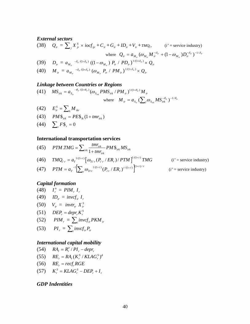
External sectors (38) = ∑ + + + + + (i’ = service industry) irQ
jSjrX × ijriocf irC irG irID irV riTMQ '
where irir
ir
ir
irir irMirMMir DMaQ δδδ ωω /1))1(( −−− −+=
(39) = irDirMa )1/( irir δδ +− )1((
irMω− irP / irPD ) )1/(1 irδ+ × irQ (40) = irM
irMa )1/( irir δδ +−irMω( irP / irPM ) )1/(1 irδ+ × irQ
Linkage between Countries or Regions (41) iririrkSSirk MPMPMSaMS ir
irk
irir
ir
)1/(1)1/( )/( θθθ ω ++−=
where irir
irkir l irkSSir MSaM θθω /1)( −−∑= (42) ∑= k ikr
Sir ME
(43) )1($$ irkikirk tmrPEPM +=
(44) ∑ =r rF 0$
International transportation services
(45) ∑ +=
irk irkirkirk
irk MSPMtmr
tmrTMGPTM $1
.
(46) [ ]1/(1 )1/(1 )' ' '( / ) /r
i r T Ti r i r rTMQ a P ER PTM TMGτω ++= (i’ = service industry)
(47) (i’ = service industry) [ τττττω/)1()1/(
')1/(1
'1 )/(
+++− ∑=r rrirTiT ERPaPTM ]
Capital formation (48) = n
rI rPIM rI(49) = irID irinvcf rI(50) = irV irinvtr S
irX(51) S
rrr KdeprDEP =(52) = rPIM iri ir PKMinvcf∑(53) = rPI iri ir Pinvcf∑ International capital mobility (54) rr
err deprPIRRA −= /
(55) φ)/( Sr
Srrr KLAGKRARE =
(56) RGErecfRE rr =(57) rr
Sr
Sr IDEPKLAGK +−=
GDP Indentities
40

(58) ∑ ∑∑ ++=i i irjrijririri irirr PNMXiocfPGMGPCMCGDPR 000
+ ∑∑ +i iriri irir PKMIDPXV 00
- ∑∑ +i iririk irkirk PEEPMMS 0$0$
(59) ∑ ∑∑ ++=i i irjrijririri irirr PNMXiocfPGMGPCMCGDPN
+ ∑∑ +i iriri irir PKMIDPXV
- ∑∑ +i iririk irkirk PEEPMMS $$
Equilibrium conditions (60) = ∑i irK S
rK
(61) = liri
L∑ SlrL
(62) Sirir DD =
(63) ' ' '$ $ /irk irk ir ir i r i r i r rik iMS PM E PE TMQ P ER F× − − −∑ ∑ $ 0=
(i’ = service industry) Walrasian law Local: (64) +−×∑ )(
iSiririr DDPD −−+ n
rrr IFS( )∑ ×i irir VP
+ rER × ' '( $ $ /irk irk ir ir i r i r r rik iMS PM E PE TMQ P ER F× − − −∑ ∑ $ ) 0=
Global: (65) +−×∑∑ ri
Sirirrr
ERDDPD /)( −−+∑ nrrrr
IFS( rr irir ERVP /)∑ × +∑ ∑ ∑∑ =−−×+−
ri k r rr rirriirirkir FTMQERPTMGPTMEMSPE 0$))/(()($ '' N.B. ∑ if and =
r rF 0$ 0)( =−∑ ∑ri k irirk EMS ∑=×r rirri TMQERPTMGPTM '' )/(
B2. Model Notation Sets i,j industries r, k countries or regions l labor types h households
41
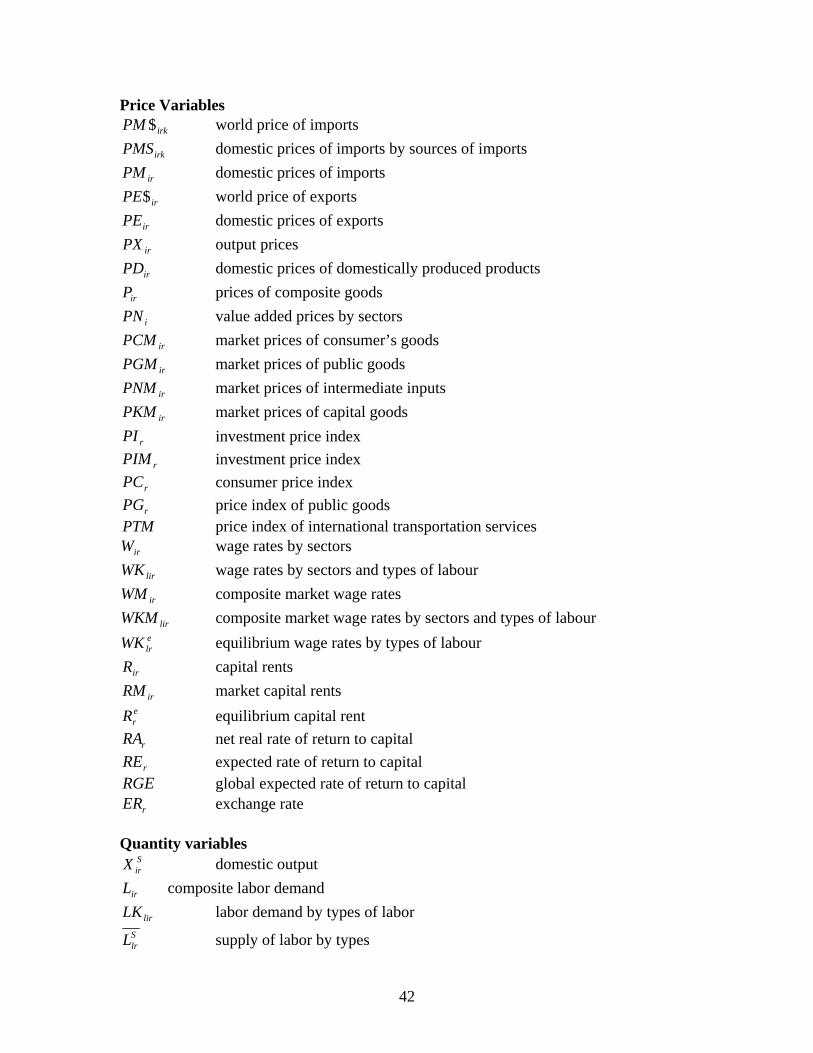
Price Variables irkPM $ world price of imports
irkPMS domestic prices of imports by sources of imports
irPM domestic prices of imports
irPE$ world price of exports
irPE domestic prices of exports
irPX output prices
irPD domestic prices of domestically produced products
irP prices of composite goods
iPN value added prices by sectors
irPCM market prices of consumer’s goods
irPGM market prices of public goods
irPNM market prices of intermediate inputs
irPKM market prices of capital goods
rPI investment price index
rPIM investment price index
rPC consumer price index
rPG price index of public goods PTM price index of international transportation services
irW wage rates by sectors
lirWK wage rates by sectors and types of labour
irWM composite market wage rates
lirWKM composite market wage rates by sectors and types of labour elrWK equilibrium wage rates by types of labour
irR capital rents
irRM market capital rents erR equilibrium capital rent
rRA net real rate of return to capital
rRE expected rate of return to capital RGE global expected rate of return to capital
rER exchange rate Quantity variables
SirX domestic output
irL composite labor demand
lirLK labor demand by types of labor SlrL supply of labor by types
42

irK capital demand by sector SrK total supply of capital
SrKLAG total capital stock in the previous period
irQ composite good demand
irD domestic supply of domestically produced products
irE export supply
irM imports
irMS imports by country of origin total demand for international transportation services
demand for international transportation services by countries and regions irTMQTMG
irC household consumption by sectors
rC total demand for household consumption
irG demand for government consumption
rG total demand for government consumption
rF$ foreign savings
rI total real fixed investment
irID demand for capital goods
irV demand for inventory investment
rDEP total depreciation expenditure
rGDPR Real GDP by countries Nominal variables
rYH household income
rYG government revenue
rSH household savings
rSG government savings
rS domestic savings nrI nominal fixed investment
rGDPN nominal GDP by countries Parameters
irXa scale parameters in production functions
irXω share parameters in production functions
irρ exponent parameters in production functions
irLa scale parameters in labour demand functions
lirLω share parameters in labour demand functions
irλ exponents in labour demand functions
43

irMa scale parameters in composite goods functions
irMω share parameters in composite goods functions
irδ exponents in composite goods functions
irSa scale parameters in import demand functions
irkSω share parameters in import demand functions
irθ exponents in import demand functions
irEa scale parameters in export supply functions
irEω share parameters in export supply functions
irγ exponents in export supply functions
ijriocf intermediate input coefficient of good j in industry i
hirykcf share of capital income accrued to household h
hlirylcf share of labor income accrued to household h
irsubs subsistence consumption (for other countries rather than Thailand)
hirsubs subsistence consumption (for Thailand)
irbshr , marginal budget shares hirbshr
ircgcf government consumption shares
irinvcf fixed investment shares
irinvtr ratios of inventory investment to real production
rPs , private saving rate hrPs
rGs government saving rate
irtm import tariff rates
irte export duty rates
irtc sale taxes on consumers’ goods
irtg sale taxes on public goods
ijrtn sale taxes on intermediate inputs
irtk sale taxes on capital goods
irtp production taxes/subsidies
lirtw labor taxes/subsidies
irtr capital taxes/subsidies
44