business cycle synchronization since 1880

Business Cycle Synchronization since 1880

Michael Artisac, George Chouliarakisbc and P.K.G. Harischandrad1

a. Centre for Economic Policy Research, London

b. Department of Economics, School of Social Sciences, University of Manchester

c. Centre for Growth and Business Cycle Research, University of Manchester

d. Central Bank of Sri Lanka

Abstract: This paper studies the behaviour of the international business cycle across 25 advanced and emerging market economies for which 125 years of annual GDP data are available. The picture that emerges is more fragmented than the one drawn by studies that focused on a narrower set of advanced market economies. The paper offers evidence in favour of a secular increase in international business cycle synchronization within a group of European and a group of English-speaking economies that started off during 1950-1973 and accelerated since 1973. Yet, in other regions of the world, country-specific shocks are still the dominant forces of business cycle dynamics. Keywords: Business Cycles; Dynamic Factor Models; Globalization; Integration JEL Classification: C32, E32, F41, N10

1 Earlier versions of this paper were presented at the International Symposium on Business Cycle Behaviour in Historical Perspective, University of Manchester, June 2009 and the 8th European Historical Economics Society Conference, Geneva, September 2009. We would like to thank the participants for their comments and suggestions. George Chouliarakis gratefully acknowledges financial support from the School of Social Sciences of the University of Manchester.

1. INTRODUCTION During the past three decades, the world economy has moved towards closer integration.

International trade flows have increased substantially, financial markets in developed and

emerging economies have become increasingly integrated, significant parts of the world

economy that were hitherto relatively insulated opened up to free trade and capital flows,

and continental European countries adopted a single currency. These developments raise the

possibility of changes not only in the properties of national business cycles but also in their

synchronization.

The large body of research that explored the effects of these structural changes on business

cycle behaviour has produced mixed results. One branch of the literature has concluded that

evidence from a wide range of industrial and developing economies does not lend strong

support to the hypothesis that increasing international trade and financial market integration

has led to an increase in the degree of business cycle synchronization (Kose et al, 2003,

2008). Another branch of the literature, focusing specifically on the experience of advanced

industrial economies, has detected the emergence of a ‘European business cycle’ since the

early 1980s (Artis and Zhang, 1997, 1999, and Artis, 2004) while more recent evidence

suggests that, as the process of international trade and financial market integration deepens,

such regional business cycle affiliations are superseded by wider business cycle clubs (Artis,

2008). Yet other studies have found that output correlations among the major industrial

countries have even decreased in the recent decades, largely on account of a remarkable cycle

of de-synchronization in the late 1980s and early 1990s (Helbling and Bayoumi, 2003, Doyle

and Faust, 2002, 2005). Overall, and despite a number of significant contributions, it would

be fair to say that the state of our knowledge about the effects of integration on cross-

national business cycle linkages remains imperfect and largely limited to the very recent

period.

The goal of this paper is to contribute towards a better understanding of the effects of

globalization on business cycle co-movements by adding to the debate a historical

dimension. To this end, the paper studies the behaviour of business cycles in 25 countries

for which at least 125 years of annual data are available. In so doing, the paper aims to

2

document some of the salient features of national business cycle behaviour and examine

changes in the pattern of cross-national business cycle synchronization over time. We know

that in many respects the countries of our sample and the historical periods that we cover

have been markedly different. They differ in terms of their institutions, their monetary and

fiscal policies, their economic structures, their natural endowments and their growth record.

The question is whether, despite these differences, the forces of economic integration that

swept the world economy during 1880-1913 and, again, since the collapse of the Bretton

Woods system of fixed exchange rates have led to greater economic interdependence and

more synchronization. Seeking an answer to this question is important for several reasons,

not least, because greater business cycle synchronization would require tighter

macroeconomic policy co-ordination during economic downturns if the experience of

beggar-thy-neighbour policies of the 1930s were to be avoided.

A variety of data and empirical methodologies suggest that the historical process of trade and

capital market integration has followed a distinctive ‘U-shape’ pattern, with momentum

peaking at the beginning and at the end of the twentieth century, but coming to a halt during

the years of the two World Wars and the Great Depression (Obstfeld and Taylor, 2003,

2004). These ebbs and flows of integration cover a period of more than a century and cut

across a wide range of international monetary regimes. The main question we address is

whether the degree of business cycle synchronization across a large number of advanced and

emerging market economies follows the same stylized ‘U-shape’ pattern. In so doing, we also

examine whether the effect of financial market integration on the international business

cycle, if any, varies with the constraints imposed on domestic macroeconomic policy by the

international monetary regime. We do so by splitting the sample in four different sub-

periods, each of which corresponds to a distinct international monetary regime

(Eichengreen 1996). The period from 1880 to 1913 corresponds to the classical Gold

Standard, a period of credible commitment to pegged exchange rates and free trade and

capital markets, often referred to as the first era of globalization of the world economy. The

period from 1920 to 1939 is characterized by the failed attempt to restore the prewar liberal

economic order in the context of a new institutional environment, the Great Depression,

and the reversal of economic integration through the introduction of trade and capital

controls. The period from 1950 to 1973 corresponds to the Bretton Woods era of fixed but

3

adjustable exchange rates and limited capital mobility as a means to prevent currency crises

and confer some degree of autonomy to domestic monetary policy. Finally, the period from

1973 onwards, an era characterized by an unprecedented rise in trade and capital market

integration, the formation of the European Monetary Union, and floating exchange rates

among the main world currencies.

In addressing the above question, our study is closely related to earlier work by Backus and

Kehoe (1992), Bergman, Bordo, and Jonung (1998), Basu and Taylor (1999), and Bordo and

Helbling (2003). These pioneering studies also examine the behaviour of business cycles over

the long run and across different exchange rate regimes. Yet, our study departs from theirs in

some fundamental ways. First, our study covers a much wider sample of countries. Unlike

earlier international comparative studies that limit themselves to a rather narrow sample of

advanced market economies, we use Barro and Ursua’s (2008) dataset and cast our net across

25 advanced and emerging market economies. The benefit from doing so is large as no other

study has looked at the effects of financial globalization on the historical properties of the

international business cycle of emerging market economies. Second, we use an unobserved

component model to estimate the business cycles of the countries of our sample. This

method has not been used before by other international and historical studies and has the

potential to significantly improve the measurement, and our understanding, of the historical

properties of the international business cycle. Third, unlike earlier work, our study explores

the channels through which financial market integration may affect the synchronization of

national business cycles. In principle, financial market integration may increase business cycle

synchronization, either by increasing the relative importance of international shocks, or by

strengthening the spillover effects across countries, e.g., through contagion. We use a Factor

Structural VAR model (Clark and Shin, 20000, Stock and Watson, 2005) to identify the

relative importance of the channels through which trade and financial integration may have

historically affected the international business cycle.

The remainder of the paper is organized as follows. Section 2 offers a discussion of the

dataset and presents the business cycle definition and measurement method that we use.

Section 3 summarizes the changes in business cycle correlations across the four sub-periods

of the sample. Section 4 uses a Factor Structural VAR model to identify the changing

4

importance of international shocks, spillovers, and country-specific shocks in driving the

international business cycle dynamics during the past 125 years. Section 5 concludes.

2. DATA AND FILTERING

The data are annual values of the logarithm of real GDP per capita and cover 25 advanced

and emerging market economies from 1880 to 2006. These economies are Austria, Belgium,

Denmark, Finland, France, Germany, Italy, Netherlands, Norway, Sweden, Switzerland,

United Kingdom, Greece, Portugal, Spain, Australia, Canada, United States, Argentina,

Brazil, Chile, Uruguay, India, Japan and Sri Lanka. The data source is Barro and Ursua

(2008) who updated Maddison’s (2003) monumental and widely used dataset by

incorporating new information from a series of recent major historical national accounts

projects and, in some occasions, provided superior estimates.

Before proceeding, a caveat is in order. We know that the quality of national accounts data

prior to World War II varies considerably across countries primarily because of differences

in the availability of raw data sources. In countries with established annual income tax

systems or statistical bureaus, the measurement of national account aggregates tends to be

more accurate than is the case elsewhere. As a result, in some cases, the ex post

reconstruction of historical national accounts is often based on extrapolations from

fragmentary raw data that cover only a narrow subset of economic activity raising, thus, the

likelihood of measurement error. Christina Romer’s (1986, 1989) criticism of prewar US

national accounts data illustrates this point very well. Although recent progress in creating

historical national accounts has significantly increased the accuracy of the data, we need to

bear this caveat in mind when interpreting results.

Our focus is on economic fluctuations over business cycle horizons. It is common to

distinguish two types of business cycles – the so-called ‘classical’ cycle and the ‘deviation’

cycle. The former is in the spirit of Burns and Mitchell’s (1946) NBER business cycle

project, where peaks are identified by being followed by absolute declines in output while

troughs by absolute increases. Such cycles are, of course, comparatively rare in growth

economies and to focus our attention only on these would lead to a paucity of observations,

5

at least, as far as the post-WWII period is concerned. The deviation cycle, by contrast, deals

with deviations in output growth from trend growth and it is this concept of the cycle that

we will use here. Thus, measuring deviation cycles requires the filtering out of the economy’s

trend growth rate. One way to do this is to use band-pass-filtered log GDP with a pass band

that only admits business cycle frequencies (periods of 1½ to 8 years). The main drawback

of this method is that a good deal of data has to be ‘thrown away’ at the two ends of the

sample. An alternative method would be to consider simple annual growth rates which use

differencing to eliminate the linear growth rate in the series. Despite the merit of simplicity,

the drawback of this method is that the trend growth rate of GDP over the past 125 years

cannot be assumed to be constant. Because a low frequency drift can introduce bias into

certain statistics used later on, such as cross-country correlations computed over sub-

samples, in our analysis, we use a flexible detrending method based on a model with a

stochastic drift (Clark 1987, Harvey and Jaeger 1993, Stock and Watson 2005). Define

as the annual growth rate of GDP. We adopt an unobserved

components specification that represents as the sum of two terms, a slowly evolving

mean growth rate (trend) and a stationary component (cycle):

)ln(100 tt GDPy

ty

ttt uy (1) where

ttt 1 (2) and ttuL (3)

Where )(L is a finite polynomial in the lag operator and L t and t are serially and

mutually uncorrelated mean zero disturbances. The Kalman smoother can be used to

estimate the trend growth rate ( t ) and the residual ( ). Obviously, the Kalman smoother

estimate of is our estimate of the deviation of GDP growth from its trend. Implementing

this detrending procedure requires a value of the ratio

tu

tu

)0(uu2 S , where is the

spectral density of at frequency zero. This ratio determines the smoothness of trend

)0(uuS

tu

6

growth and, in principle, it could be estimated by the maximum likelihood procedure.

However, when the true variance of a nonstationary state variable is nonzero but small, as it

plausibly is here, its maximum likelihood estimate is downward biased towards zero. To

avoid this so-called ‘pileup’ problem, we estimate )0(2uuS on a country-by-country basis

using the median unbiased estimator of Stock and Watson (1998) and use this country-

specific estimate to detrend GDP growth.

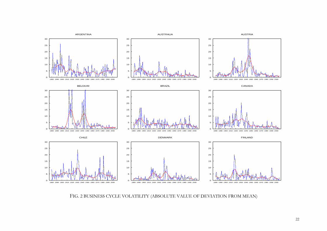
Figure 1 plots the business cycle estimates of the 25 countries of the sample. Naturally,

positive values of the estimates correspond to expansions and negative values to recessions.

The vertical lines in the United States business cycle graph indicate the business cycle

troughs as calculated by the National Bureau of Economic Research. Despite a significantly

different definition and measurement of business cycles, our below-trend-growth estimates

correspond closely to conventional chronologies of the cyclical behaviour of the US

economy. Figure 2 plots ‘raw’ estimates of the volatility of business cycles across the

countries of the sample. The segmented line in Figure 2 plots the absolute value of the

deviation of each series from its mean while the solid, smoother line is its filtered

counterpart (Hodrick-Prescott filter, smoothing parameter=100). The results present a

varied picture across countries but a recurrent theme is the considerable decline in volatility

following the end of WWII. Table 1 summarizes the changes in the standard deviation of

detrended GDP growth across countries and sub-periods and confirms that business cycle

volatility declined since 1950 in all the countries of the sample. The last column of Table 1

reports the ratio of the standard deviation of post-WWII business cycles to the standard

deviation of the pre-WWI business cycles. The data imply that business cycle volatility since

1950 has been lower than during the classical Gold Standard for 19 out of the 25 economies

of the sample.

3. CHANGES IN BUSINESS CYCLE SYNCHRONIZATION

This section reports results on the evolution of international business cycle comovements.

Tables 2-5 tabulate the correlation of detrended annual GDP growth rates across countries

for each of the four subperiods of the sample. Coefficients that are statistically significant at

7

the 10 percent level are highlighted in bold. A cursory inspection of the four Tables suggests

that the number, size and distribution of the statistically significant bilateral correlation

coefficients differs considerably across subperiods. The number of positive and statistically

significant correlation coefficients tripled between 1880-1913 and 1919-1939, fell by one-

third during the Bretton Woods era and increased by two-and-a-half times during 1973-2006.

Figure 3 plots the frequency distributions of the bilateral correlation coefficients for the four

subperiods of the sample and illustrates the shifts of the sample means. The average change

of these ‘raw’ correlations between the classical Gold Standard and the interwar period is

0.18 (from 0.02 to 0.20), the average change between the interwar years and the Bretton

Woods period is -0.06 (from 0.20 to 0.14) while the average change between Bretton Woods

and the post-1973 period is 0.10 (from 0.14 to 0.24). Are these changes over time statistically

significant? This question is very relevant since, given the relatively few observations per era,

the confidence intervals of the correlation coefficients can be relatively wide. Tables 6 and 8

report standard mean equality and non-parametric Wilcoxon Rank Sum tests suggesting that

these changes are statistically significant at the 1 percent level. The overall picture that

emerges from Tables 2-5 and Figure 3 does not lend support to the view that periods of high

trade and capital market integration are associated with increased international business cycle

comovements. During the classical Gold Standard, a period of free trade and capital

mobility, the degree of business cycle synchronization across countries is close to zero

whereas during the post-1973 period of trade and capital market integration, the mean

correlation coefficient of detrended output growth is positive but moderate. We think that

this result merits closer examination. Without precluding the likelihood of measurement

error in the prewar data, this result may point to an interpretation of the classical Gold

Standard as a period where country-specific shocks were dominant, hence, as a system that

conferred some degree of domestic policy independence. We will return to this in section 4

when we discuss the changing significance of international and country-specific shocks in

driving business cycle dynamics.

To the extent that the distribution of bilateral correlation coefficients within subperiods is

not uniform, as it is not, the size and direction of changes in average correlation coefficients

across subperiods for the country sample as a whole may hide information about patterns of

international business cycle comovements within and between country subsamples. Tables 6

8

and 8 report the evolution of mean correlation coefficients for a number of country groups

while Tables 7 and 9 report mean correlation coefficients across these groups. Two aspects

bear emphasis. First, There is compelling evidence in favour of the historical emergence of

two cyclically coherent groups. A European group that includes Austria, Belgium, France,

Germany, Italy, Netherlands and Switzerland exhibits a secular rise in its mean correlation

coefficients from a statistically insignificant value during the classical Gold Standard, to 0.24

during the interwar period, to 0.35 during the Bretton Woods years, and to 0.63 since 1973

(as the equality tests of Tables 6 and 8 suggest, under the entry ‘Core and Western European

Countries’, the mean correlation coefficient changes from the Classical Gold Standard to the

interwar period and from Bretton Woods to the post-1973 period are statistically significant

at the 1 percent level). Similarly, an Anglo-Saxon group that includes Australia, Canada, the

UK and the USA, exhibits a secular rise in its mean correlation coefficients from a

statistically insignificant 0.17 during the Classical Gold Standard and interwar years, to 0.25

during Bretton Woods and to 0.61 since 1973 (see the entry ‘Anglo-Saxon Countries’ in

Tables 6 and 8). While the mean correlation coefficients within each group have risen

sharply, the average cross-group correlation (i.e. the average correlation of each member of

the two groups with the members of the other) has fallen from 0.23 to 0.17 between the

interwar years and Bretton Woods period (although the change is not statistically significant)

and has risen only mildly to 0.32 since 1973. The secular increase in within-group average

correlation of the order of 0.40 for both groups since 1950, coupled with a rise in cross-

group correlation of just 0.09 during the same period, points towards the emergence of two

distinct groups. The origins of the two groups lie in the mid-twentieth century but their

formation process accelerated after 1973. Second, Tables 6-9 document well that no other

country group exhibits a similar secular increase in within-group or cross-group cyclical

coherence indicating that business cycle synchronization has not increased over time

universally and is not a natural consequence of closer trade and capital market integration.

Our findings lend support to earlier results by Doyle and Faust (2002), Heathcote and Perri

(2004) Kose, Prasad, and Terrones (2003) and Stock and Watson (2005) which found little

evidence in favour of increased overall synchronization during the past forty years. We now

turn to examine the proximate causes of changes in business cycle synchronization by

analyzing changes in the structure of shocks in the context of a Factor Structural VAR

model.

9

4. CHANGES IN THE IMPORTANCE OF INTERNATIONAL VS

IDIOSYNCRATIC SHOCKS

A convenient dichotomy that helps us to analyze changes in business cycle dynamics is the

dichotomy between shocks and propagation (Frisch, 1933). According to it, changes in the

dynamics of the international business cycle can be the result of changes in the nature of

shocks, changes in the transmission mechanism of shocks across countries, or a combination

of the two. Increased business cycle synchronization will then be reflected in the rising

importance of international vis-à-vis country-specific shocks or the strengthening of the

propagation mechanisms of country-specific shocks across countries (e.g. through trade and

capital flows). Identifying, thus, changes in the nature of shocks and transmission

mechanisms will cast new light in the behaviour of the international business cycle and

contribute to a better understanding of its proximate causes. The aim of this section is to do

exactly this. In particular, this section aims to measure the changes in the fractions of a

country’s cyclical variance that is due to international shocks, cross-country transmission of

country-specific shocks and idiosyncratic shocks. The basic question to be resolved is the

best way to identify an international shock and the approach taken here is to develop a

dynamic factor model in a structural VAR context (Clark and Shin 2000, Stock and Watson

2005). The model is based on the presumption that there exists a small number of common

factors that produce business cycle comovements among the economies, possibly through

trade and financial market interdependence. The common factors refer to international

shocks, therefore, it is important to distinguish between an international shock and a

country-specific shock which has some spillover effects. In FSVAR models, shocks are

identified by imposing a factor structure on the reduced form VAR innovations, such that,

an international shock is identified as a shock that affects all countries simultaneously, while

transmission of country-specific shocks affects the rest of the world with one period lag.

Because the definition of shocks depends on the frequency of data, Stock and Watson (2005)

highlight that FSVAR models may tend to misclassify shocks in studies using high frequency

data, e.g., with quarterly data, a world shock that hits one country and passes over to others

with a lag of one or more periods may be identified as a country-specific shock that has

spillover effects. However, this study is less likely to be affected by this, because we use

10

annual data, in that an international shock is most likely to have an impact within a year,

while an idiosyncratic shock may transmit to the trading partners with some lag. On the

other hand, we are aware that idiosyncratic shocks that spread to other parts of the world

within a year will be misclassified as international shocks and we bear this caveat in mind.

The basic framework of the model is described below, in that, represents annual growth

rate of per capita real GDP for country i

ty

n,...,2,1 :

nt

t

nt

t

nnn

n

nt

t

y

y

aa

aa

y

y

1

1

11

1

1111

,

where the error vector is assumed to be determined by the following factor structure:

nt

t

t

nt

t

G

11

,

where t are common international factors that affects output in all countries

simultaneously, G is a (n x k) vector of factor loadings, and i is a country-specific shock.

'ttE and 'ttE are both assumed to be diagonal. The model is estimated by using

Gaussian maximum likelihood.2 To proceed, we need to specify the lag structure for VAR

dynamics and a value for k (the number of common factors). In specifying a lag structure in

a multi-country factor model, one needs to be concerned about the dimensionality problem,

because a higher lag structure leads to a larger number of coefficients to be estimated. Two

solutions exist in the literature: first, to impose restrictions on VAR coefficients, e.g.,

specifying a different number of lags on domestic and foreign GDP growth rates, such as

VAR(4,1) as in Stock and Watson (2005) i.e., four own lags and one foreign lag. While this

option may seem to be more relevant to high frequency data, information criteria tests

suggest a VAR(1,1) specification for the present study, which seems to be consistent with

2 Results are produced in GAUSS 6.0, using an appropriately amended version of Mark Watson’s code.

11

annual data. The second option is to specify VARs for subsets of countries. This seems

reasonable given the width and length of our dataset. However, grouping countries comes

with a cost, because it tends to restrict the explanatory power of the model by limiting the

international shocks and spillover effects. Therefore, we adopt a cautious approach, in that,

we group the countries in such a way that a particular set of countries, conventionally

classified as ‘core countries’ in modern economic history, stays together all the time with

each subset of countries based on region. The core country group consists of the Anglo-

Saxon countries (Canada, UK and US) and the ‘core’ European countries (Belgium, France,

Germany, and the Netherlands). We then specify another six groups of countries: the Nordic

group (Denmark, Finland, Norway, and Sweden), the Western European group (Austria,

Italy, and Switzerland), the Southern European group (Greece, Portugal and Spain), the

Latin American group (Argentina, Brazil, Chile, Uruguay), the Asian group (India, Japan, and

Sri Lanka), and Australia. Each wave of Factor Structural VAR results consists of pooling

the core country group together with one regional group.

The other key issue in estimating FSVAR models relates to the specification of the number

of common factors (k). The literature points towards two approaches: first, formal tests can

be performed to determine k, for example, Stock and Watson (2005) propose likelihood

ratio tests, given that the FSVAR model is overidentified, in that, null hypothesis of k-factor

structure is tested against the alternative of an unrestricted VAR. The number of common

factors is determined at the level of k, which fails to reject the null. Also, Bai and Ng (2002)

suggest information criteria preferably for a larger data set. The other approach is more of

case-specific, in that, authors specify a number of k based on the empirical context of the

research study. For example, Bergman and Jonung (2010) who examine business cycle

synchronization of three Scandinavian economies impose two factors in order to allow for

estimation of the relative importance of European wide shocks and Scandinavian shocks.

Further, Bordo and Helbling (2003) who examine business cycle synchronization over

sixteen industrialized countries and across exchange rate regimes highlight opt for a one

common factor (in the static factor model).

12

In this study, we first experiment with alternative k structures, to examine how sensitive the

results are to the number of k specified. In doing so, we examine degrees of freedom issues,

pertaining to subsample estimates, as highlighted in Bordo and Helbling (2003). It turns out

that one factor model seems to produce robust results (with more degrees of freedom), yet,

without changing the results qualitatively. The degrees of freedom issue is a major concern

here because we estimate the model across subsamples, in that, we consider four sub-

samples based on historical monetary regime classifications, namely, Classical Gold Standard

(1880-1913), Interwar Gold Standard (1920-1939), Bretton Woods (1950-1972), and Post-

Bretton Woods (1973-2006). Given the definition of factor structure k=1, we estimate the

FSVAR model with 4-year ahead forecast horizon of detrended GDP growth rate over the

country groups specified above, in that, forecast errors are decomposed into: international

shocks, domestic shocks, and spillover effects, which are defined as one minus the sum of

the international and domestic shocks. By construction of the model, international and

country-specific shocks are uncorrelated, thus, the Stock and Watson (2005) procedure

produces a threefold variance decomposition of 4-year ahead forecast errors for GDP

growth in each country. Depending upon the share of error variance explained by each

component, we identify the relative importance of international shocks, country-specific

shocks and spillover effects in explaining international business cycle comovements.

Tables 10-15 summarize these variance decompositions for detrended GDP growth for the

six groups of results. At the one-year horizon, international spillovers account for none of

the business cycle forecast error variance: this is the assumption used to identify the

international shock. At longer horizons, spillovers typically account for between 10 and 40

percent of business cycle variance, depending on the country group and the sub-period. The

relative importance of international sources of fluctuations, either common shocks or

spillovers, can be measured as one minus the share of the forecast error variance attributed

to domestic shocks. A small domestic share corresponds to a relatively larger role for

international rather than domestic disturbances. Consequently, in the context of our model,

examining the hypothesis that closer trade and capital market integration increases the degree

of business cycle co-movement is tantamount to examining whether the fraction of the

forecast error variance of detrended GDP growth attributed to county-specific shocks falls

13

when integration rises. The results reported in Tables 10-15 do not offer support to this

hypothesis as, for most of the country groups of our sample, country-specific shocks do not

follow the ‘U-shaped’ pattern that is characteristic of the evolution of the trade and capital

market integration of the world economy. In particular, the relative contribution of

idiosyncratic shocks in explaining the forecast error variance of our business cycle measure

during the classical Gold Standard period is invariably high across country groups and

confirms our result in section 3 of this paper that the average correlation coefficient across

the whole country sample during this period is not statistically significantly different from

zero. This result should be interpreted with caution as the likelihood of measurement error

in the national accounts data of this period is not trivial and, to our view, this could

constitute a potential problem that needs addressing in future research. Yet, to the extent

that the data problem does not contaminate our result, this result points towards an

interpretation of the classical Gold Standard as an international monetary regime that

conferred some degree of autonomy to domestic monetary policy, e.g., a target zone.

Four salient features emerge from the historical record of business cycle synchronization as

summarized in Tables 10-15. First, the fraction of the forecast error variance of detrended

GDP growth that is due to country-specific shocks in the European Core (Belgium, France,

Germany and Netherlands) declines steadily over time. At the two-year horizon, the average

Core European fraction of cyclical variance attributed to domestic shocks declines from a

typical value of 70 percent during the Classical Gold Standard to 40 percent during the

interwar years to 35 percent during the Bretton Woods years and finally to below 30 percent

since 1973. This result holds across sub-samples and reflects mostly the increasing

importance of international shocks, and to a much lesser extent stronger transmission, in

shaping the business cycle behaviour of the European core. Second, the declining

significance of country-specific shocks is also evident in the average Western European

fraction of cyclical variance explained by domestic shocks. Indeed, the experience of

Western Europe (Italy, Austria, Switzerland) is very similar to this of the European core

suggesting that the business cycle behaviour of these seven economies is shaped to a good

extent by common international shocks. Third, the Anglo-Saxon group (Canada, UK, USA)

allows a far larger role to idiosyncratic shocks and exhibits no secular change over time. The

same is true for all four other groups, the Latin American, the Asian, the Nordic group and

14

Australia. Fourth, Table 12 shows that although the Anglo-Saxon group historically shared a

common factor with Europe, this hasn’t been the case since 1973 pointing towards a

weakening of comovements between the two country groups during the past forty years.

Indeed, this is one of the main findings of section 3 too. On the basis of the above

evidence, one can safely argue that there is no secular change in the degree of

synchronization since 1880 as many parts of the world economy do not share a common

factor and their business cycles are driven by idiosyncratic shocks. The exception to this is a

group of European countries where international shocks have played an increasingly

significant importance in shaping the behaviour of the business cycle. This result is very

much in line with the results of section 3 but qualify the conclusion of Bordo and Helbling

(2011) whose study is based on a smaller sample of countries.

5. CONCLUSIONS

This paper studies the behaviour of the international business cycle across 25 advanced and

emerging market economies for which 125 years of annual GDP data are available. The

picture that emerges is far more fragmented than the one drawn by studies that focused on a

narrower set of advanced market economies. The main results, and some directions for

future research, can be summarized as follows. First, there is compelling evidence in favour

of a secular increase in international business cycle synchronization within a group of

European and a group of English-speaking economies that started off during 1950-1973 and

accelerated since 1973. Based on the results of the Factor Structural VAR model, it is hard to

avoid the conclusion that gradual trade integration since the 1960s diminished the relative

significance of idiosyncratic shocks within a group of European countries and offered the

springboard for the formation of the European Monetary Union. Second, the secular

increase in the cyclical coherence within these two groups far outweighs the small rise in the

cyclical coherence between the two groups, thus, it would be fair to describe these two

cyclical groups as distinct. Future research should explicitly take into account the possibility

of regional common factors to allow for the emergence of distinct cyclical groups. Third, the

observed secular rise in business cycle synchronization does not extend outside this subset of

advanced market economies. In other regions of the world, country-specific shocks are still

the dominant forces of business cycle dynamics. Fourth, the lack of international business

15

cycle comovements during the Classical Gold Standard, i.e. a period of fixed exchange rates

and free trade and capital mobility, merits our attention and should act as a trigger for future

research, not least, in the direction of double-checking and improving the quality of

historical national accounts data. In this respect, very recent work in extracting information

on business cycle behaviour from less noisy economic aggregates than national accounts data

is in the right trail. Fifth, the sharp increase in business cycle synchronization during the

interwar years, as reflected in the almost universal increase in the fraction of the cyclical

variance explained by the international shock and transmission, is consistent with the view

that the Great Depression was a global monetary shock that was spread across world

through the workings of the interwar Gold Standard.

16

REFERENCES Artis, M. (2004). ‘Is There a European Business Cycle?’, in H. Siebert (ed.) Macroeconomic Policies in the World Economy, Berlin, Springer. Artis, M. (2008). ‘Europeanization or Globalization? What do Business Cycle Affiliations Say?”, in R.Shlomowitz (ed.), Flinders Essays in Economics and Economic History, Adelaide, Wakefield Press. Artis, M., and Zhang, W. (1997). ‘International Business Cycles and the ERM: Is There a European Business Cycle?’, International Journal of Finance and Economics, Vol. 2, pp. 1-16. Artis, M., and Zhang, W. (1999). ‘Further Evidence of the International Business Cycle and the ERM: Is There a European Business Cycle?’, Oxford Economic Papers, Vol. 51, pp. 120-132. Backus, D. and Kehoe, P. (1992). ‘International Evidence on the Historical Properties of Business Cycles’, American Economic Review, Vol. 82, pp. 864-888. Bai, J. and Ng, S. (2002). ‘Determining the Number of Factors in Approximate Factor Models’, Econometrica, Vol. 70, pp. 191-221. Barro, R. and Ursúa, J. (2008). ‘Macroeconomic Crises since 1870’, Brookings Papers on Economic Activity, Vol. I, pp. 255-335. Basu, S. and Taylor, A. M. (1999). ‘Business Cycles in International Historical Perspective’, Journal of Economic Perspectives, Vol. 13, pp. 45-68. Bayoumi, T., and Helbling, T. (2008). ‘Are They All in the Same Boat? The 2000-2001 Growth Slowdown and the G-7 Business Cycle Linkages’, IMF Staff Papers. Bergman, M., Bordo M. and Jonung, L. (1998). ‘Historical Evidence on Business Cycles: The International Experience’, in J.C. Fuhrer and S. Schuh (eds.), Beyond Shocks: What Causes Business Cycles? , Boston, Massachusetts, Federal Reserve Bank of Boston. Bergman, M. and Jonung, L. (2011). ‘Business Cycle Synchronization in Europe: Evidence from the Scandinavian Currency Union’, The Manchester School, Vol. 79, pp. Bordo, M., and Helbling, T. (2004) ‘Have National Business Cycles Become More Synchronized?’, in H. Siebert (ed.), Macroeconomic Policies in the World Economy, Berlin, Springer. Bordo, M. and Helbling, T. (2011). ‘International Business Cycle Synchronization in Historical Perspective’, The Manchester School, Vol. 79, pp. Kose, A., Prasad, E. and Terrones, M. (2003a). ‘How Does Globalization Affect the Synchronization of Business Cycles?’, American Economic Review, Vol. 93, pp. 57-62.

17

Kose, A., Otrok, C. and Whiteman, C. (2003b). ‘International Business Cycles: World, Region, and Country-Specific Factors’, American Economic Review, Vol. 93, pp. 1216-1239. Kose, A., Otrok, C. and Whiteman, C. (2008). ‘Understanding the Evolution of World Business Cycles’, Journal of International Economics, Vol. 75, pp. 110-130. Kose, A., Otrok, C. and Prasad, E. (2008). ‘Global Business Cycles: Convergence or Decoupling?’, NBER Working Paper 14292. Maddison, A. (2003). ‘The World Economy: Historical Statistics’, Paris, Organization of Economic Cooperation and Development. Obstfeld, M. and Taylor, A. M. (2003). ‘Globalization and Capital Markets’, in M. Bordo, A. M. Taylor and J. Williamson (eds.), Globalization in Historical Perspective, NBER, Chicago, IL, University of Chicago Press. Obstfeld, M. and Taylor, A. M. (2004). Global Capital Markets: Integration, Crisis, and Growth, Cambridge, Cambridge University Press. Ritschl, A., Sarferaz, S. and Uebele, M. (2008). ‘Output and Consumption in the Global Business Cycle 1870-2006: A Dynamic Factor Approach’, mimeo. Romer, C. (1986). ‘New Estimates of Prewar Gross National Product and Unemployment’, Journal of Economic History, Vol. 46, pp. 341-352. Romer, C. (1989). ‘The Prewar Business Cycle Reconsidered: New Estimates of Gross National Product, 1869-1908’, Journal of Political Economy, Vol. 97, pp. 1-37. Stock, J. and Watson, M. (1998). ‘Median Unbiased Estimation of Coefficient Variance in a Time-Varying Parameter Model’, Journal of the American Statistical Association, Vol. 93, pp. 349-358. Stock, J. and Watson, M. (2005). ‘Understanding Changes in International Business Cycle Dynamics’, Journal of the European Economic Association, Vol. 3, pp. 968-1006.

18

-30

-20

-10

0

10

20

1880 1890 1900 1910 1920 1930 1940 1950 1960 1970 1980 1990 2000

ARGENTINA

-30

-20

-10

0

10

20

1880 1890 1900 1910 1920 1930 1940 1950 1960 1970 1980 1990 2000

AUSTRALIA

-30

-20

-10

0

10

20

1880 1890 1900 1910 1920 1930 1940 1950 1960 1970 1980 1990 2000

AUSTRIA

-30

-20

-10

0

10

20

1880 1890 1900 1910 1920 1930 1940 1950 1960 1970 1980 1990 2000

BELGIUM

-30

-20

-10

0

10

20

1880 1890 1900 1910 1920 1930 1940 1950 1960 1970 1980 1990 2000

BRAZIL

-30

-20

-10

0

10

20

1880 1890 1900 1910 1920 1930 1940 1950 1960 1970 1980 1990 2000

CANADA

-30

-20

-10

0

10

20

1880 1890 1900 1910 1920 1930 1940 1950 1960 1970 1980 1990 2000

CHILE

-30

-20

-10

0

10

20

1880 1890 1900 1910 1920 1930 1940 1950 1960 1970 1980 1990 2000

DENMARK

-30

-20

-10

0

10

20

1880 1890 1900 1910 1920 1930 1940 1950 1960 1970 1980 1990 2000

FINLAND

FIG. 1 DETRENDED GDP GROWTH (UNOBSERVED COMPONENTS METHOD)

19

-30

-20

-10

0

10

20

1880 1890 1900 1910 1920 1930 1940 1950 1960 1970 1980 1990 2000

FRANCE

-30

-20

-10

0

10

20

1880 1890 1900 1910 1920 1930 1940 1950 1960 1970 1980 1990 2000

GERMANY

-30

-20

-10

0

10

20

1880 1890 1900 1910 1920 1930 1940 1950 1960 1970 1980 1990 2000

GREECE

-30

-20

-10

0

10

20

1880 1890 1900 1910 1920 1930 1940 1950 1960 1970 1980 1990 2000

INDIA

-30

-20

-10

0

10

20

1880 1890 1900 1910 1920 1930 1940 1950 1960 1970 1980 1990 2000

ITALY

-30

-20

-10

0

10

20

1880 1890 1900 1910 1920 1930 1940 1950 1960 1970 1980 1990 2000

JAPAN

-30

-20

-10

0

10

20

1880 1890 1900 1910 1920 1930 1940 1950 1960 1970 1980 1990 2000

NETHERLANDS

-30

-20

-10

0

10

20

1880 1890 1900 1910 1920 1930 1940 1950 1960 1970 1980 1990 2000

NORWAY

-30

-20

-10

0

10

20

1880 1890 1900 1910 1920 1930 1940 1950 1960 1970 1980 1990 2000

PORTUGAL


20

-30

-20

-10

0

10

20

1880 1890 1900 1910 1920 1930 1940 1950 1960 1970 1980 1990 2000

SPAIN

-30

-20

-10

0

10

20

1880 1890 1900 1910 1920 1930 1940 1950 1960 1970 1980 1990 2000

SRI LANKA

-30

-20

-10

0

10

20

1880 1890 1900 1910 1920 1930 1940 1950 1960 1970 1980 1990 2000

SWEDEN

-30

-20

-10

0

10

20

1880 1890 1900 1910 1920 1930 1940 1950 1960 1970 1980 1990 2000

SWITZERLAND

-30

-20

-10

0

10

20

1880 1890 1900 1910 1920 1930 1940 1950 1960 1970 1980 1990 2000

UK

-30

-20

-10

0

10

20

1880 1890 1900 1910 1920 1930 1940 1950 1960 1970 1980 1990 2000

URUGUAY

-30

-20

-10

0

10

20

1880 1890 1900 1910 1920 1930 1940 1950 1960 1970 1980 1990 2000

US


21

0

5

10

15

20

25

30

1880 1890 1900 1910 1920 1930 1940 1950 1960 1970 1980 1990 2000

ARGENTINA

0

5

10

15

20

25

30

1880 1890 1900 1910 1920 1930 1940 1950 1960 1970 1980 1990 2000

AUSTRALIA

0

5

10

15

20

25

30

1880 1890 1900 1910 1920 1930 1940 1950 1960 1970 1980 1990 2000

AUSTRIA

0

5

10

15

20

25

30

1880 1890 1900 1910 1920 1930 1940 1950 1960 1970 1980 1990 2000

BELGIUM

0

5

10

15

20

25

30

1880 1890 1900 1910 1920 1930 1940 1950 1960 1970 1980 1990 2000

BRAZIL

0

5

10

15

20

25

30

1880 1890 1900 1910 1920 1930 1940 1950 1960 1970 1980 1990 2000

CANADA

0

5

10

15

20

25

30

1880 1890 1900 1910 1920 1930 1940 1950 1960 1970 1980 1990 2000

CHILE

0

5

10

15

20

25

30

1880 1890 1900 1910 1920 1930 1940 1950 1960 1970 1980 1990 2000

DENMARK

0

5

10

15

20

25

30

1880 1890 1900 1910 1920 1930 1940 1950 1960 1970 1980 1990 2000

FINLAND

FIG. 2 BUSINESS CYCLE VOLATILITY (ABSOLUTE VALUE OF DEVIATION FROM MEAN)

22

0

5

10

15

20

25

30

1880 1890 1900 1910 1920 1930 1940 1950 1960 1970 1980 1990 2000

FRANCE

0

5

10

15

20

25

30

1880 1890 1900 1910 1920 1930 1940 1950 1960 1970 1980 1990 2000

GERMANY

0

5

10

15

20

25

30

1880 1890 1900 1910 1920 1930 1940 1950 1960 1970 1980 1990 2000

GREECE

0

5

10

15

20

25

30

1880 1890 1900 1910 1920 1930 1940 1950 1960 1970 1980 1990 2000

INDIA

0

5

10

15

20

25

30

1880 1890 1900 1910 1920 1930 1940 1950 1960 1970 1980 1990 2000

ITALY

0

5

10

15

20

25

30

1880 1890 1900 1910 1920 1930 1940 1950 1960 1970 1980 1990 2000

JAPAN

0

5

10

15

20

25

30

1880 1890 1900 1910 1920 1930 1940 1950 1960 1970 1980 1990 2000

NETHERLANDS

0

5

10

15

20

25

30

1880 1890 1900 1910 1920 1930 1940 1950 1960 1970 1980 1990 2000

NORWAY

0

5

10

15

20

25

30

1880 1890 1900 1910 1920 1930 1940 1950 1960 1970 1980 1990 2000

PORTUGAL


23

0

5

10

15

20

25

30

1880 1890 1900 1910 1920 1930 1940 1950 1960 1970 1980 1990 2000

SPAIN

0

5

10

15

20

25

30

1880 1890 1900 1910 1920 1930 1940 1950 1960 1970 1980 1990 2000

SRI LANKA

0

5

10

15

20

25

30

1880 1890 1900 1910 1920 1930 1940 1950 1960 1970 1980 1990 2000

SWEDEN

0

5

10

15

20

25

30

1880 1890 1900 1910 1920 1930 1940 1950 1960 1970 1980 1990 2000

SWITZERLAND

0

5

10

15

20

25

30

1880 1890 1900 1910 1920 1930 1940 1950 1960 1970 1980 1990 2000

UK

0

5

10

15

20

25

30

1880 1890 1900 1910 1920 1930 1940 1950 1960 1970 1980 1990 2000

URUGUAY

0

5

10

15

20

25

30

1880 1890 1900 1910 1920 1930 1940 1950 1960 1970 1980 1990 2000

US


24

2.4

FIG. 3 FREQUENCY DISTRIBUTION OF BILATERAL CORRELATION COEFFICIENTS ACROSS FOUR SUB-PERIODS

0.0

0.4

0.8

1.2

1.6

2.0

-1.00 -0.75 -0.50 -0.25 0.00 0.25 0.50 0.75

8 0 - 1 9 1 3 ) (18 2 0 - 1 9 3 9 ) (19 5 0 - 1 9 7 3 ) (19

(19 7 3 - 2 0 0 6 )

1.00

25

TABLE 1

STANDARD DEVIATION OF DETRENDED GDP GROWTH

Country Groups

1880-1913 1920-1939 1950-1973 1973-2006 19131880

19391920

sd

sd

19391920

19731950

sd

sd

19731950

20061973

sd

sd

19131880

20061950

sd

sd

Core Belgium 1.13 9.62 1.95 1.68 8.54 0.20 0.86 1.58 European France 4.16 6.32 1.39 1.30 1.52 0.22 0.93 0.32 Germany 1.87 8.82 2.59 1.63 4.71 0.29 0.63 1.08 Netherlands 2.42 5.26 2.41

1.51 2.17 0.46 0.63 0.78

Southern Greece 12.29 8.59 3.25 3.00 0.70 0.38 0.92 0.25 European Portugal 2.24 7.14 2.52 3.36 3.19 0.35 1.34 1.35 Spain 3.58 7.57 3.26

1.88 2.12 0.43 0.58 0.68

Western Austria 2.12 6.51 2.77 1.59 3.07 0.43 0.57 0.98 European Italy 1.30 4.07 1.45 2.20 3.13 0.36 1.52 1.46 Switzerland 3.94 4.18 2.25 1.98 1.06 0.54 0.88 0.53

Anglo-Saxon Australia 6.09 4.42 2.06 1.81 0.72 0.47 0.88 0.31 Canada 4.59 8.31 2.32 2.12 1.81 0.28 0.91 0.48 UK 2.45 3.99 1.46 1.90 1.63 0.37 1.31 0.70 US 4.41 7.22 2.63 1.97 1.64 0.36 0.75 0.51

Nordic Denmark 1.47 3.60 2.28 1.89 2.45 0.63 0.83 1.39 Finland 3.15 4.35 2.75 2.76 1.38 0.63 1.01 0.87 Norway 1.54 5.01 1.53 1.56 3.25 0.31 1.02 1.01 Sweden 2.95 4.77 1.63 1.84 1.62 0.34 1.12 0.59

Asian India 5.32 3.25 2.85 2.75 0.61 0.87 0.97 0.52 Japan 5.42 5.50 2.44 2.11 1.01 0.44 0.86 0.41 Sri Lanka 5.32 4.89 2.17 2.74 0.92 0.44 1.26 0.47

Latin Argentina 9.28 4.59 4.39 5.75 0.49 0.96 1.31 0.56 American Brazil 6.81 4.62 3.00 3.75 0.68 0.65 1.25 0.51 Chile 5.35 9.19 3.07 5.97 1.72 0.33 1.95 0.89 Uruguay 8.70 9.88 5.00 5.77 1.14 0.51 1.15 0.63

26

TABLE 2

CROSS-COUNTRY CORRELATIONS OF DETRENDED GDP GROWTH 1880-1913

BEL FRA GER NETH AUST ITA SWITZ GRE POR SPA DEN FIN NOR SWE IND JAP SLK ARG BRA CHL URU AUSL CAN UK US BE L 01. 0 FRA 0.23 1.00 GER -0.40 -0.09 1.00 NETH 0.19 -0.06 -0.14 1.00 AUST -0.06 0.37 0.07 -0.12 1.00 ITA -0.21 0.14 -0.02 -0.04 0.21 1.00 SWITZ 0.32 -0.20 -0.21 -0.11 -0.09 -0.27 1.00 GRE 0.06 0.16 0.09 0.04 0.15 -0.27 0.22 1.00 POR 0.00 -0.09 0.13 -0.46 0.10 0.07 0.29 0.02 1.00 SPA 0.02 0.22 -0.26 0.10 0.04 -0.03 -0.01 -0.23 -0.15 1.00 DEN 0.14 0.03 -0.22 -0.22 0.05 0.16 0.01 -0.10 0.18 0.05 1.00 FIN 0.14 0.07 0.28 -0.19 -0.06 0.09 -0.06 -0.18 0.33 -0.31 0.29 1.00 NOR 0.16 0.00 -0.07 -0.01 -0.18 -0.10 0.18 -0.28 -0.07 0.22 -0.17 -0.05 1.00 SWE -0.28 -0.07 0.26 -0.22 0.10 0.08 0.13 -0.14 0.28 0.06 0.15 0.16 0.27 1.00 IND 0.13 -0.15 -0.07 0.19 -0.17 -0.06 0.26 0.05 0.14 0.25 -0.07 -0.05 0.05 -0.03 1.00 JAP 0.21 0.19 0.00 -0.11 0.33 -0.06 0.13 -0.04 0.12 0.36 0.09 0.31 -0.12 0.09 0.19 1.00 SLK 0.42 0.21 -0.17 -0.30 0.32 0.20 0.05 -0.29 0.36 0.06 0.37 0.12 0.07 0.12 0.07 0.13 1.00 ARG -0.02 0.06 0.20 0.26 -0.07 -0.22 -0.05 0.34 -0.31 -0.15 -0.08 0.01 -0.28 0.08 -0.33 -0.03 -0.24 1.00 BRA -0.11 -0.02 -0.26 -0.08 0.26 -0.01 0.11 -0.17 0.07 0.14 0.25 0.19 -0.06 -0.03 -0.11 0.19 -0.07 -0.14 1.00 CHL 0.15 -0.02 -0.22 -0.08 0.32 0.20 0.06 0.05 -0.02 0.11 -0.04 -0.07 0.10 -0.17 -0.21 0.16 0.26 -0.12 0.22 1.00 URU -0.33 -0.04 -0.04 0.14 -0.24 0.17 -0.20 0.19 -0.10 -0.12 -0.23 0.06 0.11 0.17 -0.09 -0.24 -0.33 0.24 -0.22 0.01 1.00 AUSL 0.06 0.13 0.03 0.18 0.13 0.14 -0.38 -0.03 -0.14 -0.11 -0.16 0.06 -0.21 -0.06 -0.21 0.09 0.04 -0.05 0.02 0.08 -0.03 1.00 CAN 0.04 0.14 -0.28 0.07 0.25 0.02 0.10 -0.02 0.13 0.22 -0.09 -0.22 0.18 0.04 0.32 -0.09 0.15 -0.33 0.39 -0.06 -0.23 -0.07 1.00 UK 0.30 0.39 -0.04 0.38 0.25 -0.11 -0.02 -0.01 -0.08 0.00 -0.11 0.14 0.14 -0.02 -0.20 0.07 0.11 0.17 0.24 0.07 -0.19 0.24 0.39 1.00 US 0.34 -0.03 -0.53 0.24 -0.03 0.00 0.34 -0.17 -0.02 0.30 0.17 -0.12 -0.03 -0.14 0.17 -0.08 0.03 -0.04 0.43 0.04 -0.33 -0.19 0.40 0.22 1.00

Note: Figures in bold indicate statistical significance at the 10 percent level.

27

TABLE 3


BEL FRA GER NETH AUST ITA SWITZ GRE POR SPA DEN FIN NOR SWE IND JAP SLK ARG BRA CHL URU AUSL CAN UK US BEL 1.00 FRA 0.38 1.00 GER 0.19 0.24 1.00 NETH 0.59 0.32 0.47 1.00 AUST 0.20 0.45 0.72 0.57 1.00 ITA -0.60 0.01 0.11 -0.15 0.12 1.00 SWITZ 0.47 0.78 0.12 0.12 0.19 -0.20 1.00 GRE 0.34 0.04 0.53 0.30 0.29 -0.26 0.00 1.00 POR 0.05 0.11 -0.02 0.10 -0.02 -0.10 0.32 -0.19 1.00 SPA 0.15 0.14 0.03 0.15 0.18 -0.04 0.28 0.15 0.35 1.00 DEN 0.21 0.61 -0.17 -0.10 0.03 -0.15 0.66 -0.26 0.11 0.01 1.00 FIN 0.52 0.33 0.32 0.23 0.16 -0.22 0.56 -0.09 0.19 0.01 0.21 1.00 NOR 0.16 0.43 0.21 -0.17 0.04 0.06 0.56 0.03 0.01 -0.01 0.49 0.27 1.00 SWE 0.09 0.64 0.33 -0.15 0.25 0.02 0.58 0.08 -0.06 -0.01 0.73 0.20 0.68 1.00 IND -0.49 0.10 0.10 0.19 0.28 0.40 -0.39 -0.17 -0.13 -0.09 -0.24 -0.31 -0.20 -0.13 1.00 JAP -0.46 -0.13 0.32 0.14 0.30 0.60 -0.35 0.03 -0.16 -0.08 -0.40 -0.32 -0.25 -0.26 0.43 1.00 SLK -0.24 0.37 0.23 -0.04 0.22 0.20 0.27 0.09 0.24 0.02 0.09 0.29 0.18 0.31 0.35 0.01 1.00 ARG 0.38 0.57 0.46 0.41 0.42 0.02 0.66 0.12 0.21 0.23 0.44 0.64 0.27 0.44 -0.17 -0.01 0.40 1.00 BRA 0.44 0.29 0.34 0.28 0.10 -0.15 0.53 -0.10 0.00 -0.11 0.27 0.78 0.33 0.24 -0.29 0.00 0.06 0.66 1.00 CHL 0.29 0.42 0.43 0.20 0.33 -0.03 0.52 0.26 -0.05 -0.01 0.30 0.62 0.30 0.32 -0.15 0.11 0.45 0.78 0.59 1.00 URU -0.22 0.16 0.27 0.06 0.41 0.19 0.09 -0.15 -0.07 0.00 0.29 0.21 0.28 0.35 0.38 -0.13 0.40 0.39 0.15 0.22 1.00 AUSL 0.06 0.12 0.48 0.26 0.25 0.28 0.09 -0.03 0.03 -0.02 -0.25 0.50 0.03 -0.03 0.04 0.40 0.28 0.54 0.47 0.52 0.07 1.00 CAN 0.00 0.43 0.47 0.04 0.45 0.39 0.50 -0.04 0.01 0.03 0.37 0.48 0.64 0.62 -0.05 -0.06 0.47 0.60 0.42 0.46 0.65 0.33 1.00 UK -0.47 0.12 0.28 -0.25 0.15 0.52 0.17 -0.26 0.15 -0.05 0.02 0.27 0.39 0.26 0.28 0.19 0.49 0.35 0.20 0.34 0.57 0.40 0.63 1.00 US 0.02 0.47 0.35 0.16 0.35 0.36 0.34 -0.08 -0.07 -0.18 0.49 0.37 0.32 0.61 0.04 0.07 0.46 0.66 0.36 0.57 0.43 0.34 0.70 0.46 1.00


28

TABLE 4


BEL FRA GER NETH AUST ITA SWITZ GRE POR SPA DEN FIN NOR SWE IND JAP SLK ARG BRA CHL URU AUSL CAN UK US BEL 1.00 FRA 0.55 1.00 GER 0.02 0.14 1.00 NETH 0.60 0.33 0.33 1.00 AUST 0.32 0.69 0.47 0.34 1.00 ITA 0.00 0.11 0.28 0.04 0.16 1.00 SWITZ 0.71 0.60 0.37 0.46 0.62 0.23 1.00 GRE 0.54 0.07 -0.16 0.23 0.08 -0.15 0.29 1.00 POR 0.53 -0.02 -0.41 0.39 -0.08 -0.32 0.25 0.47 1.00 SPA 0.13 0.03 -0.27 -0.43 -0.25 -0.09 -0.09 0.08 -0.17 1.00 DEN 0.33 0.34 -0.03 0.40 0.03 0.02 0.14 0.16 0.07 -0.27 1.00 FIN 0.59 0.47 0.27 0.27 0.37 0.04 0.62 0.16 0.08 0.17 0.21 1.00 NOR 0.44 0.29 -0.09 0.27 0.11 -0.16 0.49 0.25 0.28 0.14 0.33 0.38 1.00 SWE 0.49 0.39 0.08 0.37 0.34 0.18 0.50 0.16 0.01 -0.03 0.46 0.40 0.12 1.00 IND 0.06 -0.02 0.12 0.27 0.05 0.28 0.00 -0.11 -0.22 -0.05 0.01 -0.07 -0.10 0.32 1.00 JAP 0.37 0.39 0.10 0.10 0.10 0.56 0.31 -0.05 -0.10 0.16 0.19 0.36 0.07 0.31 0.17 1.00 SLK 0.14 0.40 0.12 0.10 0.25 0.47 0.17 -0.16 -0.27 0.08 0.02 0.06 0.00 0.16 0.28 0.66 1.00 ARG 0.35 0.43 0.04 0.42 0.36 -0.18 0.12 0.45 0.23 0.00 0.26 0.29 0.07 0.11 0.13 0.05 0.13 1.00 BRA -0.08 -0.04 0.07 -0.11 0.15 0.04 -0.04 -0.18 0.10 -0.21 0.10 0.25 -0.27 -0.18 -0.20 0.04 -0.06 0.02 1.00 CHL -0.09 0.12 -0.18 -0.13 -0.11 0.19 -0.14 0.04 -0.04 0.00 -0.08 -0.32 0.03 -0.37 -0.15 0.13 0.26 -0.14 -0.08 1.00 URU 0.54 0.57 0.46 0.43 0.61 0.33 0.58 0.25 0.01 -0.27 0.20 0.34 0.16 0.26 0.03 0.29 0.32 0.19 0.01 0.37 1.00 AUSL 0.11 0.01 -0.08 0.27 0.16 0.03 0.11 0.30 0.14 -0.10 -0.02 0.09 -0.05 0.37 0.03 0.19 0.16 0.27 -0.18 -0.26 -0.09 1.00 CAN 0.23 0.10 0.14 0.07 -0.10 -0.20 0.12 0.19 0.08 0.18 -0.06 -0.18 0.07 -0.22 -0.28 0.13 0.13 -0.07 -0.21 0.13 0.01 -0.04 1.00 UK 0.45 0.25 0.30 0.64 0.49 0.10 0.49 0.27 0.28 -0.45 0.30 0.30 0.27 0.50 0.17 0.22 0.00 0.16 -0.06 -0.21 0.40 0.50 -0.11 1.00 US 0.25 0.14 0.22 0.09 0.06 0.07 0.28 0.17 0.05 -0.09 0.17 -0.05 0.20 0.02 -0.43 0.30 0.25 -0.24 -0.20 0.15 0.28 0.14 0.70 0.30 1.00


29

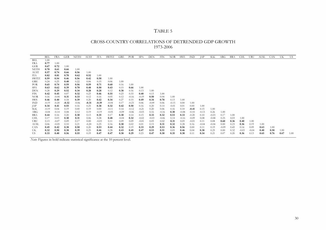
TABLE 5


BEL FRA GER NETH AUST ITA SWITZ GRE POR SPA DEN FIN NOR SWE IND JAP SLK ARG BRA CHL URU AUSL CAN UK US BEL 1.00 FRA 0.77 1.00 GER 0.67 0.72 1.00 NETH 0.70 0.61 0.66 1.00 AUST 0.57 0.74 0.66 0.56 1.00 ITA 0.82 0.81 0.70 0.62 0.52 1.00 SWITZ 0.59 0.54 0.46 0.56 0.42 0.58 1.00 GRE 0.24 0.25 0.40 0.22 0.06 0.15 0.06 1.00 POR 0.65 0.74 0.59 0.56 0.59 0.71 0.60 0.16 1.00 SPA 0.63 0.62 0.39 0.70 0.48 0.50 0.43 0.15 0.66 1.00 DEN 0.28 0.29 0.52 0.34 0.28 0.28 0.12 0.38 0.16 0.13 1.00 FIN 0.42 0.45 0.07 0.32 0.23 0.46 0.55 0.23 0.33 0.40 0.13 1.00 NOR 0.16 -0.04 0.31 0.33 0.12 0.16 0.05 0.12 -0.16 -0.19 0.50 0.04 1.00 SWE 0.46 0.40 0.18 0.39 0.20 0.42 0.34 0.27 0.15 0.49 0.34 0.78 0.13 1.00 IND -0.19 -0.20 -0.32 -0.06 -0.31 -0.39 -0.04 0.17 -0.23 0.06 -0.09 0.06 -0.15 0.00 1.00 JAP 0.34 0.41 0.55 0.16 0.25 0.38 0.32 0.42 0.50 0.16 0.20 0.14 -0.01 0.01 0.00 1.00 SLK -0.19 0.04 0.19 0.00 0.19 0.00 -0.11 0.14 -0.12 -0.21 0.20 0.06 0.16 0.10 -0.41 0.15 1.00 ARG -0.04 -0.14 0.08 0.12 0.19 -0.19 -0.05 -0.09 -0.06 -0.03 0.16 -0.16 0.30 -0.08 -0.10 -0.13 0.26 1.00 BRA 0.44 0.16 0.20 0.30 0.13 0.35 0.17 0.30 0.14 0.15 0.33 0.32 0.53 0.33 -0.20 0.10 -0.03 0.17 1.00 CHL 0.17 0.03 0.30 0.31 0.06 0.28 0.48 -0.04 0.32 -0.02 -0.03 -0.06 0.14 -0.16 -0.09 0.08 -0.08 0.25 0.03 1.00 URU 0.13 -0.07 0.09 0.17 0.00 -0.03 0.11 0.09 0.09 -0.01 0.05 0.02 0.31 0.05 -0.01 0.11 0.08 0.60 0.36 0.40 1.00 AUSL 0.06 -0.05 0.10 0.21 -0.20 0.25 0.16 0.30 0.02 0.01 0.15 0.31 0.32 0.28 0.16 -0.04 -0.04 0.00 0.23 0.36 0.19 1.00 CAN 0.45 0.42 0.38 0.50 0.20 0.53 0.44 0.32 0.19 0.33 0.29 0.53 0.36 0.56 0.00 0.11 0.19 -0.09 0.45 0.14 0.09 0.63 1.00 UK 0.32 0.50 0.38 0.39 0.25 0.46 0.28 0.43 0.45 0.47 0.53 0.51 0.05 0.46 0.04 0.38 0.25 0.00 0.32 -0.03 -0.04 0.40 0.58 1.00 US 0.33 0.40 0.56 0.55 0.19 0.47 0.47 0.38 0.29 0.23 0.47 0.30 0.35 0.30 0.11 0.34 0.21 0.07 0.20 0.36 0.13 0.65 0.76 0.67 1.00


30

TABLE 6

EQUALITY TESTS OF AVERAGE WITHIN-GROUP CORRELATION COEFFICIENTS ACROSS SUB-PERIODS

1880-1913(a) & 1920-1939(b)

1920-1939 & 1950-1973(c)

1950-1973 & 1973-2006(d)

t-test [p-value] Mean(a) Mean(b) t-test

[p-value] Mean(c) t-test

[p-value] Mean(d)

All Countries -9.29 [0.00]

0.02 (0.01)

0.20 (0.02)

2.84 [0.00]

0.14 (0.01)

-5.28 [0.00]

0.24 (0.01)

Core European -3.66 [0.00]

-0.04 (0.09)

0.37 (0.06)

0.32 [0.75]

0.33 (0.09)

-3.77 [0.00]

0.69 (0.02)

Core & Western European -3.20 [0.00]

-0.02 (0.04)

0.24 (0.07)

-1.27 [0.21]

0.35 (0.05)

-5.17 [0.00]

0.63 (0.02)

Core & Southern European -4.05 [0.00]

-0.03 (0.04)

0.21 (0.04)

0.85 [0.40]

0.14 (0.07)

-4.68 [0.00]

0.53 (0.05)

Core & Southern European (excld. Greece)

-3.79 [0.00]

-0.05 (0.05)

0.22 (0.04)

1.01 [0.32]

0.12 (0.09)

-5.83 [0.00]

0.64 (0.02)

Core, Western & Southern European -3.81 [0.00]

-0.01 (0.03)

0.18 (0.04)

-0.02 [0.99]

0.18 (0.05)

-6.49 [0.00]

0.53 (0.03)

Core, Western & Southern European (excld. Greece)

-3.69 [0.00]

-0.02 (0.03)

0.19 (0.04)

0.08 [0.94]

0.18 (0.05)

-7.74 [0.00]

0.61 (0.02)

Nordic -2.62 [0.03]

0.11 (0.07)

0.43 (0.10)

1.05 [0.32]

0.31 (0.05)

-0.05 [0.96]

0.32 (0.12)

Anglo-Saxon 0.00 [1.00]

0.17 (0.10)

0.17 (0.10)

-0.50 [0.63]

0.25 (0.13)

-2.67 [0.02]

0.61 (0.05)

Latin American -3.63 [0.00]

0.00 (0.08)

0.47 (0.10)

3.17 [0.01]

0.06 (0.08)

-2.15 [0.06]

0.30 (0.08)

Asian -0.98 [0.38]

0.13 (0.03)

0.26 (0.13)

-0.53 [0.62]

0.37 (0.15)

2.01 [0.11]

-0.09 (0.17)

Note: Standard errors in parentheses. The European Core includes Belgium, France, Germany and the Netherlands; the Western European group includes Austria, Italy, and Switzerland; the South European group includes Greece, Portugal and Spain; the South European group (excl. Greece) includes Portugal and Spain only; the Nordic group includes Denmark, Finland, Norway and Sweden; the Latin American group includes Argentina, Brazil, Chile and Uruguay; the Asian group includes India, Japan and Sri Lanka; the Anglo-Saxon group includes Australia, Canada, the UK and the USA.

31

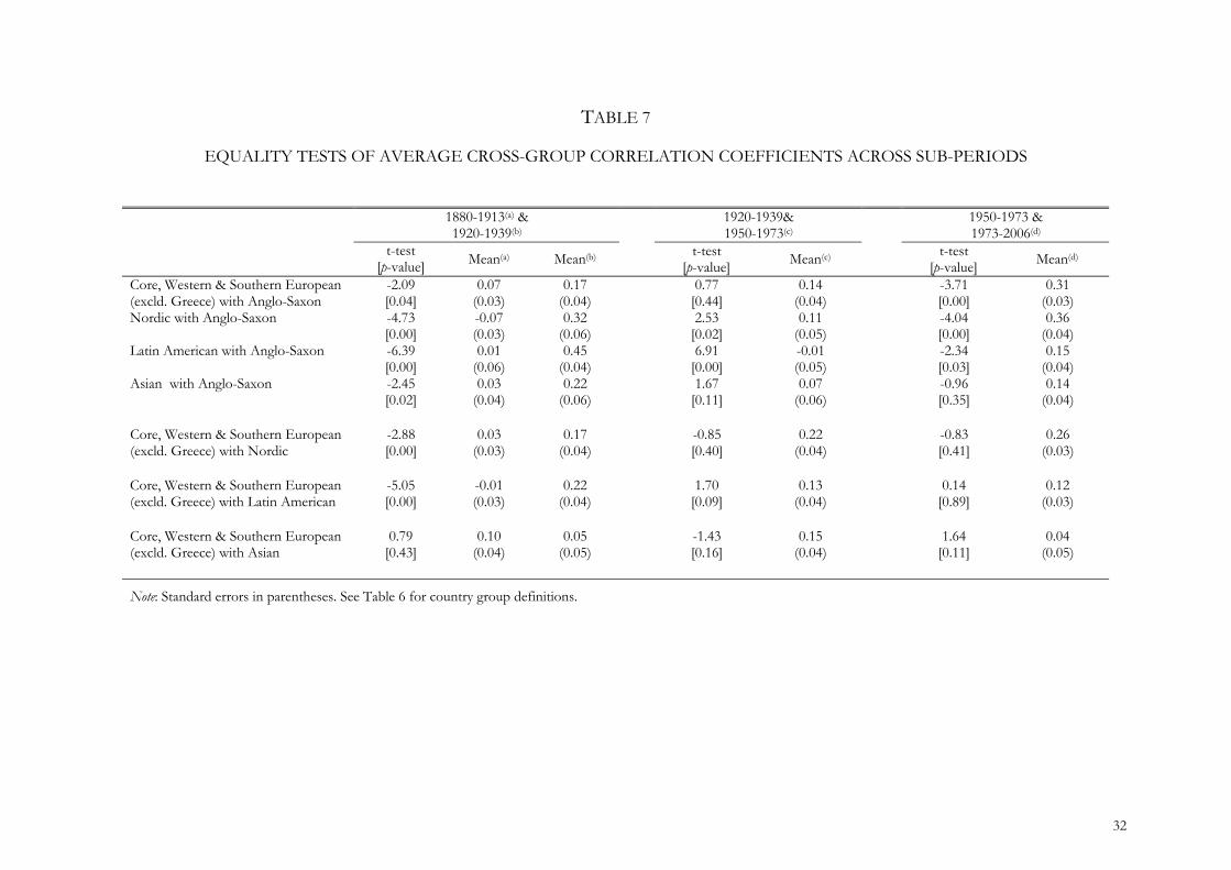
TABLE 7

EQUALITY TESTS OF AVERAGE CROSS-GROUP CORRELATION COEFFICIENTS ACROSS SUB-PERIODS

1880-1913(a) &

1920-1939(b) 1920-1939&

1950-1973(c) 1950-1973 &

1973-2006(d) t-test

[p-value] Mean(a) Mean(b) t-test [p-value]

Mean(c) t-test [p-value]

Mean(d)

Core, Western & Southern European (excld. Greece) with Anglo-Saxon

-2.09 [0.04]

0.07 (0.03)

0.17 (0.04)

0.77 [0.44]

0.14 (0.04)

-3.71 [0.00]

0.31 (0.03)

Nordic with Anglo-Saxon -4.73 [0.00]

-0.07 (0.03)

0.32 (0.06)

2.53 [0.02]

0.11 (0.05)

-4.04 [0.00]

0.36 (0.04)

Latin American with Anglo-Saxon -6.39 [0.00]

0.01 (0.06)

0.45 (0.04)

6.91 [0.00]

-0.01 (0.05)

-2.34 [0.03]

0.15 (0.04)

Asian with Anglo-Saxon -2.45 [0.02]

0.03 (0.04)

0.22 (0.06)

1.67 [0.11]

0.07 (0.06)

-0.96 [0.35]

0.14 (0.04)

Core, Western & Southern European (excld. Greece) with Nordic

-2.88 [0.00]

0.03 (0.03)

0.17 (0.04)

-0.85 [0.40]

0.22 (0.04)

-0.83 [0.41]

0.26 (0.03)

Core, Western & Southern European (excld. Greece) with Latin American

-5.05 [0.00]

-0.01 (0.03)

0.22 (0.04)

1.70 [0.09]

0.13 (0.04)

0.14 [0.89]

0.12 (0.03)

Core, Western & Southern European (excld. Greece) with Asian

0.79 [0.43]

0.10 (0.04)

0.05 (0.05)

-1.43 [0.16]

0.15 (0.04)

1.64 [0.11]

0.04 (0.05)

Note: Standard errors in parentheses. See Table 6 for country group definitions.

32

TABLE 8

NON-PARAMETRIC EQUALITY TESTS OF AVERAGE WITHIN-GROUP CORRELATION COEFFICIENTS ACROSS SUB-PERIODS

1880-1913(a) & 1920-1939(b)

1920-1939& 1950-1973(c)

1950-1973 & 1973-2006(d)

Test value [p-value] Median(a) Median (b) Test value

[p-value] Median(c) Test value

[p-value] Median(d)

All Countries 8.56 [0.00]

0.02 0.21 2.93 [0.00]

0.13 4.95 [0.00]

0.23

Core European 8.56 [0.00]

-0.08 0.35 0.08 [0.94]

0.33 2.80 [0.01]

0.69

Core & Western European 2.96 [0.00]

-0.06 0.20 1.03 [0.30]

0.33 3.85 [0.00]

0.62

Core & Southern European (excld. Greece)

3.07 [0.00]

-0.06 0.15 0.87 [0.38]

0.13 3.40 [0.00]

0.66

Core, Western & Southern European (excld. Greece)

3.60 [0.00]

-0.02 0.15 0.04 [0.97]

0.19 5.82 [0.00]

0.61

Nordic 1.84 [0.07]

0.15 0.38 0.72 [0.47]

0.35 0.08 [0.94]

0.24

Anglo-Saxon -0.08 [0.94]

0.23 0.23 0.40 [0.69]

0.22 1.84 [0.07]

0.64

Latin American 2.32 [0.02]

-0.05 0.49 2.32 [0.02]

0.02 1.84 [0.07]

0.30

Asian 0.44 [0.66]

0.13 0.35 0.00 [1.00]

0.28 1.75 [0.08]

0.00

Note: Results are based on the Wilcoxon Rank Sum Test. See Table 6 for country group definitions.

33

TABLE 9

NON-PARAMETRIC EQUALITY TESTS OF AVERAGE CROSS-GROUP CORRELATION COEFFICIENTS ACROSS SUB-PERIODS

1880-1913(a) & 1920-1939(b)

1920-1939 & 1950-1973(c)

1950-1973 & 1973-2006(d)

Test value [p-value] Median(a) Median (b) Test value

[p-value] Median(c) Test value

[p-value] Median(d)

Core, Western & Southern European (excld. Greece) with Anglo-Saxon

2.13 [0.03]

0.06 0.15 0.82 [0.41]

0.11 3.59 [0.00]

0.33

Nordic with Anglo-Saxon

3.45 [0.00]

-0.04 0.37 2.36 [0.02]

0.08 3.33 [0.00]

0.34

Latin American with Anglo-Saxon 4.16 [0.00]

-0.01 0.47 4.35 [0.00]

-0.07 2.05 [0.04]

0.13

Asian with Anglo-Saxon 1.88 [0.06]

0.06 0.23 1.24 [0.21]

0.14 0.32 [0.75]

0.13

Core, Western & Southern European (excld. Greece) with Nordic

2.18 [0.03]

0.05 0.13 1.11 [0.27]

0.27 0.91 [0.36]

0.28

Core, Western & Southern European (excld. Greece) with Latin American

4.27 [0.00]

-0.02 0.25 1.60 [0.11]

0.06 0.43 [0.66]

0.12

Core, Western & Southern European (excld. Greece) with Asian

0.47 [0.64]

0.13 0.10 0.99 [0.32]

0.12 1.54 [0.12]

0.00

Note: Results are based on the Wilcoxon Rank Sum Test. See Table 6 for country group definitions.

34

TABLE 10

VARIANCE DECOMPOSITIONS BASED ON THE ONE-FACTOR FSVAR: INTERNATIONAL SHOCKS, SPILLOVERS, AND IDIOSYNCRATIC SHOCKS

1880-1913 1920-1939 1950-1973 1973-2006

Fraction of Forecast Error variance due to:




Country Groups

Horizon

Int’l shocks

Spillo- vers

Own shocks

Int’l shocks

Spillo- vers

Own shocks

Int’l shocks

Spillo- vers

Own shocks

Int’l shocks

Spillo- vers

Own shocks

Nordic 1 0.03 0.00 0.97 0.03 0.00 0.97 0.39 0.00 0.61 0.17 0.00 0.83 2 0.03 0.17 0.80 0.05 0.40 0.56 0.33 0.38 0.29 0.07 0.13 0.80 3 0.03 0.23 0.74 0.09 0.42 0.49 0.32 0.44 0.23 0.04 0.27 0.69 4 0.02 0.26 0.71 0.10 0.44 0.45 0.36 0.43 0.22 0.03 0.36 0.61 Core 1 0.16 0.00 0.84 0.41 0.00 0.59 0.56 0.00 0.44 0.71 0.00 0.30 European 2 0.16 0.14 0.71 0.33 0.36 0.32 0.59 0.13 0.29 0.65 0.10 0.26 3 0.14 0.19 0.68 0.31 0.44 0.26 0.59 0.18 0.24 0.57 0.16 0.26 4 0.14 0.21 0.65 0.28 0.50 0.22 0.59 0.19 0.22 0.50 0.23 0.26 Anglo- 1 0.49 0.00 0.51 0.51 0.00 0.49 0.24 0.00 0.76 0.29 0.00 0.71 Saxon 2 0.43 0.12 0.45 0.41 0.30 0.29 0.26 0.13 0.62 0.18 0.15 0.66 3 0.42 0.17 0.40 0.40 0.34 0.25 0.28 0.18 0.54 0.11 0.29 0.61 4 0.41 0.22 0.37 0.39 0.38 0.23 0.30 0.21 0.50 0.09 0.37 0.55 Notes: The Nordic country group includes Denmark, Norway and Sweden. The European Core includes Belgium, France, Germany and the Netherlands. The Anglo-Saxon group includes Canada, the UK and the US. Results refer to simple averages over country groups.

35

TABLE 11


1880-1913 1920-1939 1950-1973 1973-2006





Country Groups

Horizon

Int’l shocks

Spillo- vers

Own shocks

Int’l shocks

Spillo- vers

Own shocks

Int’l shocks

Spillo- vers

Own shocks

Int’l shocks

Spillo- vers

Own shocks

Latin 1 0.19 0.00 0.81 0.26 0.00 0.74 0.16 0.00 0.84 0.01 0.00 0.99 American 2 0.18 0.15 0.68 0.34 0.28 0.38 0.14 0.24 0.62 0.02 0.16 0.82 3 0.17 0.21 0.62 0.33 0.39 0.28 0.14 0.30 0.55 0.01 0.26 0.72 4 0.17 0.24 0.59 0.30 0.47 0.23 0.13 0.32 0.55 0.01 0.34 0.65 Core 1 0.16 0.00 0.84 0.44 0.00 0.56 0.43 0.00 0.57 0.70 0.00 0.31 European 2 0.15 0.16 0.70 0.42 0.18 0.40 0.37 0.21 0.42 0.63 0.10 0.27 3 0.13 0.23 0.64 0.43 0.24 0.33 0.30 0.38 0.32 0.57 0.18 0.25 4 0.12 0.26 0.62 0.43 0.27 0.30 0.25 0.49 0.27 0.53 0.24 0.24 Anglo- 1 0.49 0.00 0.51 0.44 0.00 0.56 0.16 0.00 0.84 0.34 0.00 0.66 Saxon 2 0.42 0.17 0.40 0.37 0.34 0.30 0.12 0.21 0.68 0.19 0.20 0.61 3 0.41 0.23 0.36 0.32 0.51 0.17 0.10 0.33 0.58 0.11 0.35 0.54 4 0.41 0.27 0.32 0.26 0.63 0.11 0.09 0.38 0.53 0.08 0.42 0.50 Notes: The Latin American group includes Argentina, Brazil and Uruguay. See Table 10 for definitions of the European Core and Anglo-Saxon groups. Results refer to simple averages over country groups.

36

TABLE 12


1880-1913 1920-1939 1950-1973 1973-2006





Country Groups

Horizon

Int’l shocks

Spillo- vers

Own shocks

Int’l shocks

Spillo- vers

Own shocks

Int’l shocks

Spillo- vers

Own shocks

Int’l shocks

Spillo- vers

Own shocks

Western 1 0.06 0.00 0.94 0.26 0.00 0.74 0.47 0.00 0.53 0.51 0.00 0.49 European 2 0.04 0.25 0.71 0.13 0.24 0.63 0.45 0.18 0.37 0.53 0.13 0.33 3 0.05 0.29 0.66 0.13 0.34 0.53 0.43 0.27 0.30 0.47 0.25 0.28 4 0.04 0.33 0.63 0.12 0.42 0.45 0.39 0.37 0.24 0.44 0.30 0.26 Western 1 0.02 0.00 0.99 0.05 0.00 0.96 0.48 0.00 0.52 0.60 0.00 0.40 European 2 0.04 0.14 0.82 0.07 0.09 0.84 0.41 0.19 0.41 0.63 0.14 0.23 (excl. 3 0.05 0.18 0.78 0.10 0.21 0.70 0.37 0.31 0.33 0.57 0.24 0.20 Switzerland) 4 0.05 0.22 0.74 0.09 0.33 0.58 0.32 0.42 0.27 0.54 0.28 0.18 Core 1 0.11 0.00 0.90 0.52 0.00 0.48 0.55 0.00 0.45 0.71 0.00 0.29 European 2 0.10 0.21 0.69 0.39 0.29 0.32 0.58 0.16 0.27 0.56 0.15 0.29 3 0.10 0.27 0.63 0.40 0.33 0.28 0.56 0.21 0.23 0.45 0.28 0.28 4 0.10 0.30 0.60 0.38 0.37 0.25 0.53 0.26 0.21 0.39 0.34 0.27 Anglo- 1 0.45 0.00 0.55 0.39 0.00 0.61 0.44 0.00 0.56 0.12 0.00 0.88 Saxon 2 0.40 0.13 0.48 0.39 0.33 0.28 0.44 0.09 0.47 0.05 0.13 0.82 3 0.37 0.21 0.42 0.33 0.43 0.24 0.44 0.13 0.43 0.04 0.24 0.73 4 0.35 0.26 0.38 0.28 0.54 0.18 0.44 0.16 0.40 0.04 0.28 0.68 Notes: The Western European group includes Austria, Italy and Switzerland. See Table 10 for definitions of the European Core and Anglo-Saxon groups. Results refer to simple averages over country groups.

37

TABLE 13


1880-1913 1920-1939 1950-1973 1973-2006





Country Groups

Horizon

Int’l shocks

Spillo- vers

Own shocks

Int’l shocks

Spillo- vers

Own shocks

Int’l shocks

Spillo- vers

Own shocks

Int’l shocks

Spillo- vers

Own shocks

Southern 1 0.01 0.00 0.99 0.18 0.00 0.82 0.54 0.00 0.46 0.31 0.00 0.69 European 2 0.01 0.31 0.68 0.15 0.33 0.52 0.45 0.23 0.31 0.23 0.11 0.67 3 0.02 0.39 0.59 0.14 0.37 0.49 0.53 0.23 0.24 0.19 0.20 0.61 4 0.02 0.40 0.58 0.12 0.38 0.50 0.56 0.25 0.20 0.17 0.26 0.57 Southern 1 0.01 0.00 0.99 0.24 0.00 0.77 0.53 0.00 0.47 0.44 0.00 0.57 European 2 0.01 0.32 0.68 0.20 0.37 0.44 0.45 0.16 0.39 0.33 0.10 0.58 (excl. 3 0.03 0.39 0.59 0.19 0.40 0.41 0.49 0.20 0.32 0.27 0.18 0.55 Greece) 4 0.03 0.41 0.57 0.17 0.42 0.42 0.53 0.21 0.27 0.24 0.24 0.53 Core 1 0.17 0.00 0.83 0.27 0.00 0.74 0.52 0.00 0.49 0.67 0.00 0.33 European 2 0.15 0.15 0.70 0.18 0.39 0.44 0.55 0.14 0.31 0.54 0.19 0.27 3 0.13 0.25 0.63 0.19 0.47 0.35 0.54 0.26 0.20 0.41 0.37 0.22 4 0.12 0.28 0.61 0.18 0.53 0.30 0.52 0.33 0.15 0.33 0.48 0.19 Anglo- 1 0.43 0.00 0.57 0.51 0.00 0.49 0.22 0.00 0.78 0.13 0.00 0.87 Saxon 2 0.36 0.17 0.48 0.51 0.23 0.26 0.21 0.15 0.64 0.05 0.18 0.77 3 0.33 0.29 0.38 0.51 0.27 0.23 0.23 0.21 0.57 0.03 0.30 0.66 4 0.32 0.33 0.35 0.48 0.33 0.19 0.24 0.24 0.51 0.03 0.35 0.62 Notes: The South European group includes Greece, Portugal and Spain. See Table 10 for definitions of the European Core and Anglo-Saxon groups. Results refer to simple averages over country groups.

38

TABLE 14


1880-1913 1920-1939 1950-1973 1973-2006





Country Groups

Horizon

Int’l shocks

Spillo- vers

Own shocks

Int’l shocks

Spillo- vers

Own shocks

Int’l shocks

Spillo- vers

Own shocks

Int’l shocks

Spillo- vers

Own shocks

Asian 1 0.02 0.00 0.98 0.06 0.00 0.94 0.21 0.00 0.79 0.07 0.00 0.93 2 0.04 0.33 0.63 0.13 0.20 0.67 0.23 0.14 0.64 0.07 0.17 0.76 3 0.04 0.42 0.54 0.15 0.29 0.57 0.23 0.22 0.55 0.07 0.25 0.69 4 0.03 0.44 0.52 0.14 0.32 0.54 0.21 0.29 0.50 0.07 0.30 0.64 Core 1 0.16 0.00 0.84 0.46 0.00 0.54 0.59 0.00 0.41 0.64 0.00 0.36 European 2 0.15 0.12 0.74 0.42 0.23 0.35 0.59 0.16 0.25 0.55 0.17 0.29 3 0.14 0.15 0.70 0.41 0.29 0.31 0.55 0.27 0.18 0.47 0.27 0.26 4 0.14 0.17 0.69 0.40 0.33 0.28 0.51 0.35 0.14 0.42 0.34 0.24 Anglo- 1 0.48 0.00 0.52 0.51 0.00 0.49 0.40 0.00 0.60 0.37 0.00 0.63 Saxon 2 0.41 0.11 0.47 0.52 0.24 0.24 0.41 0.22 0.37 0.19 0.25 0.55 3 0.39 0.16 0.44 0.50 0.34 0.17 0.39 0.30 0.31 0.12 0.44 0.45 4 0.39 0.19 0.42 0.43 0.43 0.13 0.36 0.38 0.26 0.09 0.50 0.40 Notes: The Asian group includes India, Japan and Sri Lanka. See Table 10 for definitions of the European Core and Anglo-Saxon groups. Results refer to simple averages over country groups.

39

TABLE 15


1880-1913 1920-1939 1950-1973 1973-2006





Country Groups

Horizon

Int’l shocks

Spillo- vers

Own shocks Int’l

shocks Spillo- vers

Own shocks Int’l

shocks Spillo- vers

Own shocks Int’l

shocks Spillo- vers

Own shocks

Australia 1 0.00 0.00 1.00 0.05 0.00 0.95 0.22 0.00 0.78 0.02 0.00 0.98 2 0.01 0.10 0.89 0.10 0.02 0.88 0.18 0.26 0.56 0.01 0.06 0.93 3 0.02 0.09 0.89 0.13 0.05 0.83 0.16 0.31 0.53 0.01 0.08 0.91 4 0.02 0.10 0.88 0.14 0.06 0.80 0.14 0.37 0.49 0.01 0.09 0.90 Core 1 0.15 0.00 0.85 0.39 0.00 0.61 0.56 0.00 0.44 0.69 0.00 0.31 European 2 0.14 0.11 0.75 0.27 0.30 0.45 0.64 0.06 0.30 0.63 0.09 0.27 3 0.14 0.15 0.72 0.25 0.41 0.34 0.65 0.10 0.26 0.56 0.19 0.25 4 0.14 0.16 0.70 0.24 0.48 0.29 0.64 0.13 0.23 0.50 0.26 0.25 Anglo- 1 0.44 0.00 0.56 0.23 0.00 0.77 0.32 0.00 0.68 0.27 0.00 0.73 Saxon 2 0.39 0.14 0.47 0.16 0.34 0.49 0.34 0.08 0.58 0.18 0.10 0.72 3 0.38 0.19 0.43 0.11 0.48 0.42 0.35 0.10 0.54 0.13 0.18 0.69 4 0.37 0.23 0.40 0.08 0.59 0.33 0.37 0.13 0.51 0.10 0.23 0.67 Notes: See Table 10 for definitions of the European Core and Anglo-Saxon groups. Results refer to simple averages over country groups.

40

business cycle synchronization since 1880

Documents