bulletin of the university of utah volume 52 october …
TRANSCRIPT
........... BULLETIN OF THE UNIVERSITY OF UTAH
Volume 52 October 1961
Bulletin No. 108
of the
UTAH ENGINEERING EXPERIMENT STATION
G R A V I T Y F L O W O F B U L K S O L I D S
by
A. W. Jenike
Salt Lake City, Utah
/
No. 29
PREFACE
There is hardly an industry in existence which does not use
solid materials in bulk form. Where the volume of the solids is
substantial, gravity is usually relied upon to cause the solids
to flow. Such materials as ores, coal, cement, flour, cocoa,
soil, to which the general term of bulk solids is applied, flow
by gravity or are expected to flow by gravity in thousands of
installations and by the billions of tons annually. Mining relies
on gravity flow in block-caving and in ore passes; subsidence is
a case of gravity flow of solids. Agriculture relies on gravity
flow of its products in storage silos, in feed plants and on the
farms. Every type of processing industry depends on gravity flow
of some solid, often of several solids.
Although vast quantities of bulk solids have been handled
for many years, the author believes that this is the first compre
hensive study of the subject. The fact that this work appears
at this time is not accidental, but stems from the progress achieved
during the past fifteen years in the mathematical theory of plas
ticity and in the techniques of numerical calculation. On the basis
of recently developed and refined principles of plasticity, the
problem of flow of bulk solids has been set up in mathematical terms.
A few years ago, this would not have been possible; just as a few years
ago the mathematically formulated problem would have been practically
insoluble because there were no computers to carry out the necessary

calculations.
The careful reader of the author’s previous reports and papers on
the subject of flow of bulk solids will notice substantial modifica
tions in the design formulae. No apology is offered for these seeming
inconsistencies; the author has always approached the subject from the
standpoint of the engineer who has had to provide definite recommenda
tions on the basis of information at hand, at the time. Hence, as
the volume of experience increased, the theory was developed, and the
numerical data were computed, the design methods improved and changed -
at times, radically*
The work is presented in six parts. In Part I, the yield function
applicable to bulk solids is described, and the flow properties of
bulk solids are defined. The solids are assumed to be rigid-plastic,
isotropic, frictional, and cohesive. During incipient failure, the
solids expand (dilate), during steady state flow, they may expand or
contract. The yield function is consistent with the principle of
normality [7] which is specifically applied in incipient failure.
Part II contains the theory of steady state gravity flow of
solids in converging and vertical channels. The equations are first
derived in a general form, applicable to problems of extrusion as well
as gravity flow, in plane strain and in axial symmetry. Some of the
derivations are more general than they need to be for this work.
They will be referred to in other publications which are now in pre
paration [22, 23]. It is shown that, provided the slopes of the walls
of a converging channel are sufficiently steep and mathematically
continuous, the stress pattern in the neighborhood of the vertex of
the channel is, primarily, a function of the slope and of the fric
tional conditions of the walls at the vertex, with the influence of
the top boundary of the channel vanishing at the vertex . The parti
cular stress field which develops at the vertex is called the radial
stress field, because it is the field which can lead to a radial
velocity field.
Since the radial stress field is closely approached in the
vicinity of the vertex, that field represents the stresses at the
outlet of a channel. The region of the outlet of a channel is most
important because it is there, that obstructions to flow originate.
The radial stress field thus provides a basis for a general solution
of flow in this important region of the channels.
In Part III, the conditions leading to incipient failure are
considered. General equations of stress are derived in plane strain
and in axial symmetry. The conditions following incipient failure
are discussed, and it is suggested that the velocity fields usually
computed for conditions of failure are meaningless and that only
initial acceleration fields can be computed. Two cases of incipient
failure are analyzed: doming across a flow channel, and piping (which
refers to a state of stress around a vertical, empty hole of circular
cross-section).
Part IV describes the flow criteria. The material developed in
the previous three parts is brought together to relate the slopes of
channels and the size of the outlets necessary to maintain the flow of

a solid of given flowability on walls of given frictional properties.
Part V describes the testing apparatus and the method which has
been developed to measure the flowability of solids, their density, and
the angle of friction between a solid and a wall.
Finally, Part VI contains the application of the theory to the
design of storage installations and flow channels, and discusses flow
promoting devices, feeders, segregation, blending, structural problems,
the flow of ore, as well as aspects of block-caving and miscellaneous
items related to the gravity flow of solids. All these topics are
approached from the standpoint of flow: their effect on flow and
vice-versa.
The reader will soon realize that many of the bins now in opera
tion have been designed to fill out an available space at a minimum
cost of the structure rather than to satisfy the conditions of flow.
The result has been a booming business for manufacturers of flow
promoting devices. While there are, and always will be, solids which
are not suitable for gravity flow, the vast majority of them will flow
if the bins and feeders are designed correctly. However, a correct
bin will usually be taller and more expensive. It is up to the
engineer to decide whether the additional cost of the correct bin
will be balanced by savings in operation.
This part is made as self-contained as possible to facilitate
its reading to the engineer who has neither time nor inclination to
study the theoretical parts.
The reader versed in soil mechanics should note that the magnitude
iv

of the stresses discussed here is 100 to 1000 times smaller than that
encountered in soil mechanics. Hence, some phenomena which may not
even be observable in soil mechanics assume critical importance in
the gravity flow of solids. For instance, the curvature of the yield
loci (Mohr envelopes) in the ( cf, t ) coordinates is seldom detectable
in soil mechanics, but in gravity flow the curvature assumes an import
ant role in the determination of the flowability of a solid. By the
terminology of soil mechanics, solids possessing a cohesion of 50 pounds
per square foot are cohesionless: standard soil mechanics tests do
not measure such low values. But a solid with that value of cohesion,
an angle of internal friction of 30°, and a weight of 100 pounds
per cubic foot can form a stable dome across a 3-foot-diameter channel
and prevent flow from starting. In gravity flow, it is of interest
to be able to predict whether or not flow will take place through a
6-inch-diameter orifice. This involves values of cohesion down to 8
pounds per square foot and even less for lighter solids.
v

ACKNOWLEDGEMENTS
The work described in this report has been carried out over a
period of some nine years, and during that time the author has become
indebted to a number of persons who have contributed of their time
and skills, and to a number of institutions which for the past five
years have given financial support to the project.
The author is particularly grateful to Dr. P. J. Elsey of the
Utah Engineering Experiment Station for his constant and sympathetic
interest in the project, and to Dr. Elsey and Professor R. H. Woolley
for their assistance in setting up the Bulk Solids Flow Laboratory
at the University of Utah; to Professor R. T. Shield of Brown Univer
sity for the many long discussions of the topics of plasticity and
for his critical revues of the work at various stages of advancement.
The author is very much in debt to his students: Joseph L. Taylor,
who has contributed of his mathematical skill, and, especially, Jerry
R. Johanson, whose constant assistance in every facet of the work has
been most useful. Mr. Johanson, a Ph.D. candidate, also carried
out all of the numerical calculations which this work required.
The cost of this project has been substantial and the author
wishes to acknowledge the initial support which he received from
the American Institute of Mining Mineralogical and Petroleum Engineers,
whose Mineral Beneficiation and Research Committees promptly recommended
the author’s application for AIME sponsorship. This was followed by
a grant of money from Engineering Foundation and by the further support
from research funds of the Utah Engineering Experiment Station.
The AIME and the Engineering Foundation have remained sponsors of the
project.
Sincere thanks are due to Dr. Carl J. Christensen, director of
the Utah Engineering Experiment Station, for his help in keeping the
project alive through times of financial difficulty.
The main support for the applied part of the project, entitled
"Bulk Solids Flow", has come from the American Iron and Steel Institute
to whom the author is most grateful.
The mathematical concepts described in this report, as well as
other work which is appearing separately, have been developed under
a 1959 grant from the National Science Foundation to a project entitled
"Flow of rigid-plastic solids in converging channels under the action
of body forces".
Andrew W. Jenike October, 1961
vii

CONTENTS
PART I - THE YIELD FUNCTION 1
Introduction 1The coordinate system 5Effective yield locus 9Stresses and density during flow 10Yield locus 15Time yield locus 22Stresses during failure 22Flow-function 24Flowfactor 26Wall yield locus 28
PART II - STEADY STATE FLOW 35General equations 35
Stress field 35Velocity field 37
Superposition 40Physical conditions 40Grids, special lines and regions 42
Converging channels 57Equations of stress 57Radial stress field 59
Derivation 59Solutions of the radial stress field 63Resultant vertical force 68
Stresses at the walls 84Influence of compressibility 84
General stress field 107 Proof of convergence to a radial
stress field at the vertex 107Boundaries 114
viii

Radial velocity field 119Vertical channels 124
Stress field 128Velocity field 132
PART III - INCIPIENT FAILURE 135
General equations 135Stress field 137Initial acceleration field 138
Superposition 143Physical conditions 143Grids and special lines 143
Doming 145Piping 148
PART IV - FLOW CRITERIA 156
Introduction 156No-doming 156
Plane and axial symmetry 157Plane asymmetry 158Flowfactor plots 160Influence of compressibility 160
No-piping 176
PART V - TESTING THE FLOW PROPERTIES OF BULK SOLIDS 182
Apparatus 182Testing 186
Continuous flow 186(a) Representative specimen 186(b) Uniform specimen 188(c) Flow 190(d) Shear 195 Example 198
ix
. Time effect 202Density 204Plots of flow properties 204Angle of friction ’ 206
PART VI - DESIGN 208Introduction 208Flow properties of bulk solids 209Limitations of the analysis 217Types of flow 218
Mass flow 219Hopper& with one vertical wall 228P uig f low 230
Calculations of the dimensions of the outlet 231(a) Doming 231
' (d) Piping . 234(c) Particle interlocking ' 236
Influence of dynamic over-pressures 236- Flow ptomor.ing devices 242Examples of design for, flow 248Feeders 268
Feeder Loads 272Belt feeder 274Side-discharge reciprocating feeder 278
Segregation and blending in flow 282Flooding 286Heat transfer 288Gas counterflow 288Structural problems 292
Stresses acting on hopper walls 292Bin failures 292
Ore 294. Broken rock 294
x

Coarse ore 301Block-caving 304
REFERENCES 307
xi

PART I
THE YIELD FUNCTION
' Introduction
In gravity flow of solids, as in soil mechanics, it is convenient
to assume pressures and compressive strain rates as positive, and
tensions and expansive strain rates as negative. This convention is
adopted throughout the work.
The solids which are considered in this work are rigid-plastic.
In the plastic regions, the solids are assumed to be isotropic, fric
tional, cohesive and compressible. During incipient failure an element
of a solid expands, while during steady state flow, the element either
expands or contracts as does the pressure along the streamline.
While many problems of continuous plastic flow have been solved
for isotropic, non-work-hardening solids with a zero angle of friction
[e.g., 1,2,3,4,5], attempts to work out solutions of continuous
flow of solids, which exhibit an angle of friction greater than zero,
have not been successful. The cause of the difficulty has lain in
the yield function ascribed to these solids. The yield function was
a generalization of the criterium of either Tresca or von Mises into
a function dependent on the hydrostatic stress. In the principal
stress space such a generalization transformed the prism of Tresca
and the cylinder of von Mises into, respectively, a pyramid and a cone,
-1 -

which were assumed to be of constant size and to extend without a bound
in the direction of the hydrostatic pressure. As a result, the princi
ple of plastic potential [6], or normality [7], required the solid to
dilate continuously during flow while at the same time retaining its
strength properties. Continuous dilation is not supported by physical
observations. Dilation implies a reduction in density which in turn
causes a loss of strength and a shrinking of the yield surface.
There is ample evidence obtained from shear and triaxial tests
to the effect that a solid may flow without a change of density as
well as with an increase of density, and that during flow the yield
surface of an element of the solid at a generic point is remarkably
independent of the history of stress and strain [8].
In this work a yield surface recently proposed by Jenike and
Shield [9] is used, This surface is shown in Fig. 1, in principal
stress space. The abscissa a£v/2 = is in the cr , c^-p lane and
bisects the angle between the a^c^-axes. This surface is the
Shield's pyramid [10] with three modifications: the pyramid is bounded
on the pressure side (after Drucker [11])by a flat hexagonal base
perpendicular to the octahedral axis; the size of the pyramid is a
function of the density, the time interval of consolidation at rest,
the temperature, and the moisture content of the solid; and the vertex
of the pyramid is rounded off.
During flow, the time interval of consolidation is zero, while
the temperature and moisture content are assumed constant; density is
variable and is assumed a function of the major pressure at a generic
-2-
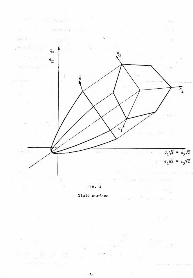
Fig. 1
Yield surface
-3 -

point. In consequence, the size of the yield surface during flow is
a function of the major pressure only, while the change in the size
of the yield surface (and in density) of an element becomes a function
of the gradient of the major pressure along the path of that element.
A change of density is measured by the normal component of the
strain rate vector, which thus must be free to assume a positive or
a negative direction depending on the sign of the pressure gradient,
and independently of the state of stress at the generic point. The
adopted yield surface allows this freedom to the strain rate vector
because, during flow, the vector is located at a corner between the
side walls of the pyramid and its flat, hexagonal base, as shown in
Fig. 1. In the plane strain flow of an incompressible solid, normality
locates the stresses on a straight side of the hexagonal base off the
yield surface. In the plane strain flow of a compressible solid and
in axi-symmetric flow, which involve three dimensional deformations,
normality locates the stresses at a corner of the hexagonal base.
It will thus be observed that in axial symmetry the principles
of isotropy and plastic potential enforce the Haar and von Karman
hypothesis [12] for the adopted yield function, except possibly when
the principal stresses in the meridian plane are either both major
or both minor. However, the latter conditions exclude all fields
with body force*, hence are useless in this work. The Haar and
* Assume the meridian pressures to be both minor, then equations (14) - (16) and (20) - (22) become
a = a = ct0 = a(l - sin 6), t =0, cr = a, = a( 1 + sin 6) x y 2 xy (X 1
-4-
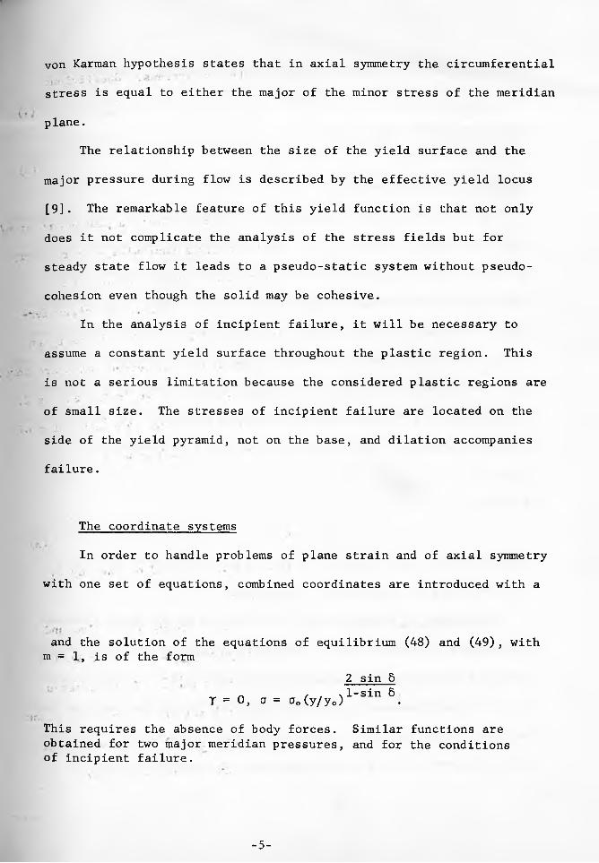
von Karman hypothesis states that in axial symmetry the circumferential
stress is equal to either the major of the minor stress of the meridian
plane.
The relationship between the size of the yield surface and the
major pressure during flow is described by the effective yield locus
[9]. The remarkable feature of this yield function is that not only
does it not complicate the analysis of the stress fields but for
steady state flow it leads to a pseudo-static system without pseudo
cohesion even though the solid may be cohesive.
In the analysis of incipient failure, it will be necessary to
assume a constant yield surface throughout the plastic region. This
is not a serious limitation because the considered plastic regions are
of small size. The stresses of incipient failure are located on the
side of the yield pyramid, not on the base, and dilation accompanies
failure.
The coordinate systems
In order to handle problems of plane strain and of axial symmetry
with one set of equations, combined coordinates are introduced with a
and the solution of the equations of equilibrium (48) and (49), with m = 1, is of the form
2 sin S„ _ / , \1-sin 6T = 0 , a = a0 (y/y0) .
This requires the absence of body forces. Similar functions are obtained for two major meridian pressures, and for the conditions of incipient failure.
-5-
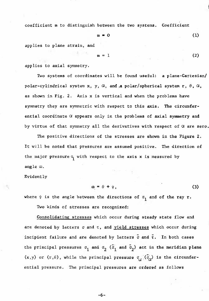
coefficient m to distinguish between the two systems. Coefficient
m — 0
applies to plane strain, and
m = 1
applies to axial symmetry.
Two systems of coordinates will be found useful: a plane-Cartesian/
polar-cylindrical system x, y, OC, and ,a polar/spherical system r, 6, Ct,
as shown in Fig. 2. Axis x is vertical and when the problems have
symmetry they are symmetric with respect to this axis. The circumfer
ential coordinate OC appears only in the problems of axial symmetry and
by virtue of that symmetry all the derivatives with respect of OC are zero.
The positive directions of the stresses are shown in the Figure 2.
It will be noted that pressures are assumed positive. The direction of
the major pressure a with respect to the axis x is measured by
angle g o .
Evidently
co = e + t, ' (3)
where \|r is the angle between the directions of and of the ray r.
Two kinds of stresses are recognized:
Consolidating stresses which occur during steady state flow and
are denoted by letters a and t, and yield stresses which occur during
incipient failure and are denoted by letters a and x. In both cases
the principal pressures and and a act in the meridian plane
(x,y) or (r,9), while the principal pressure a' (cL) is the circumfer-Ct c*ential pressure. The principal pressures are ordered as follows
(2)
(1)
-6 -
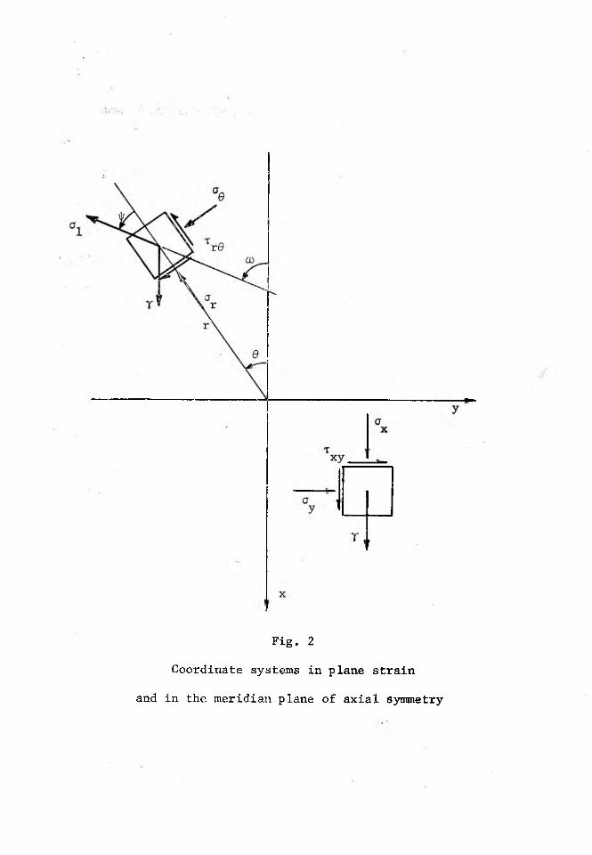
Fig. 2
Coordinate systems in plane strain
and in the meridian plane of axial symmetry

(4)
The assumed yield function is of the following general form
( 5 )
where T is the bulk density of the solid, t the time interval of
consolidation at rest, T its temperature, and H its surface moisture
content„
It should be noted that the method by which a solid is consolidat
ed to the given density T may affect the yield function. For instance,
a solid may be consolidated by vibration, or pounding; it may be
consolidated by the application of a hydrostatic pressure, as well as
by the application of pressures which are different in magnitude but
whose deviator components are insufficient to cause shear. Then,
and this is of main interest in our study, a solid may be consolidated
under a set of pressures which cause a continuous deformation of the
solid: this is the condition of flow. Finally, flow may be stopped
for an interval of time t with the consolidating pressures remaining
practically unchanged and with the solid undergoing additional con
solidation at rest.
The bulk density of a solid is assumed to be a function of the
majore consolidating pressure o , as well as of the time t, the temp
erature T, and the moisture content H, thus
T = T(J15t,T,H). (6)
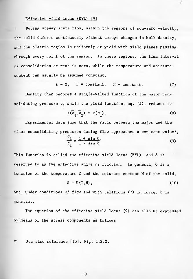
Effective yield locus (EYL) [9]
During steady state flow, within the regions of non-zero velocity,
the solid deforms continuously without abrupt changes in bulk density,
and the plastic region is uniformly at yield with yield planes passing
through every point of the region. In these regions, the time interval
of consolidation at rest is zero, while the temperature and moisture
content can usually be assumed constant,
t = 0, T = constant, H = constant. (7)
Density then becomes a single-valued function of the major con
solidating pressure while the yield function, eq. (5), reduces to
f (a1 5a2) = FCap . (8)
Experimental data show that the ratio between the major and the
minor consolidating pressures during flow approaches a constant value*,« 1 + sin 5.
ct2 1 - sin 5 w
This function is called the effective yield locus (EYL), and 6 is
referred to as the effective angle of friction. In general, 5 is a
function of the temperature T and the moisture content H of the solid,
5 = S (T, H) , (10)
but, under conditions of flow and with relations (7) in force, 6 is
constant.
The equation of the effective yield locus (9) can also be expressed
by means of the stress components as follows
* See also reference [13], Fig. 1.2.2.
-9-

sin 5 = v ' * J -------(11)
or
1 xQ i x 2V + S' <i1
+ ay
J
p r - v2 + 4t 2r 9li Q +(1 2)
In principal stress space, function (9) is represented by the
side OAB of Shield's pyramid [10] with its vertex at the origin, Fig. 3.
This pyramid is also of hexagonal cross-section but, unlike the yield
function, Fig. 1, extends into the direction of hydrostatic pressure
without a base. In the (cj,t) coordinates this function is represented
by two straight lines, EYL passing through the origin and inclined at
the angle S to the cr-axis, Fig. 4. These lines are envelopes of
Mohr stress circles determining the consolidating pressures and
1 ■ Stresses and density during flow '
It is convenient to introduce a mean pressure "a .+ a „ a + a a +an ,1 2 x y r Qa - . (13)
The component stresses can now be expressed in the plane-Cartesian/
polar-cylindrical coordinates by
a = a(l + sin 8 cos 2oo) , (14)
a = a(l - sin 5 cos 2a>) , (15)
T = o sin & sin 2a>: (16)xy ’ v '
-10-

Fig. 3
Effective yield surface
-11-

and in the polar/spherical coordinates by
cr = a(l + sin 6 cos , (17)
Oq = a(l - sin 6 cos 2v|/) , (18)
T Q = o sin 8 sin . (19)rt7
The principal pressures are
= a(1 + sin 5), (20)
a2 = o(l - sin 8), (21)
Oq, = a( 1 + k sin 8), (22)
where
k = + 1, (23)
for converging flow, locates the stresses on the edge OA of the pyramid,
Fig. 3, while
k = -1, (24)
for diverging flow, locates the stresses on the edge OB of the pyramid.
On the strength of the relations (6), (7) and (20), the bulk
density during flow becomes of the form
r = r(a) . (25)
This relation has been found experimentally to be well represented
by the equation
T = To(l + a)? (26)
where To and (3 are constant under conditions of flow. Tests show that
for a measured in pounds per square foot, (3 does not exceed,10. The
method of measuring g is described in reference [14] and the results of
-12-

Fig. 4
Effective yield locus
Fig. 5
Yield loci
-13-
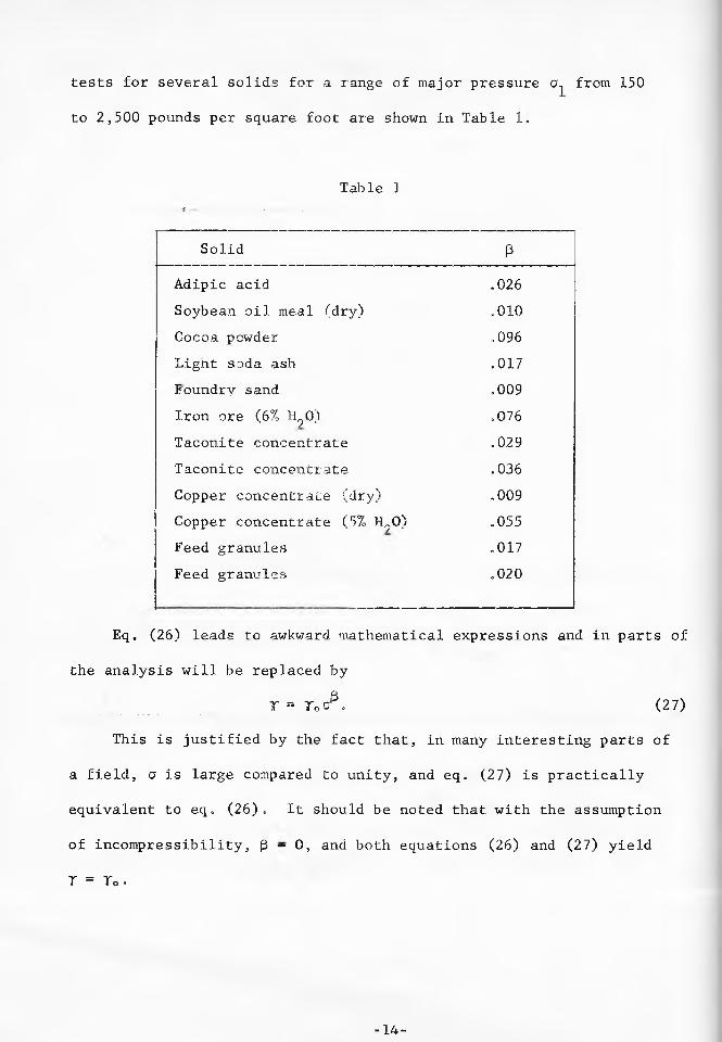
tests for several solids for a range of major pressure cr from 150
to 2,500 pounds per square foot are shown in Table 1.
Table 1* £ • - ........ i .... .
Solid PAdipic acid .026Soybean oil meal (dry) .010
Gocoa powder .096Light soda ash .017Foundry sand .009Iron ore (6% H^O) .076Taconite concentrate .029Taconite concentrate .036Copper concentrate (dry) .009Copper concentrate (57o H?0) .055Feed granules .017Feed granules .020
Eq. (26) leads to awkward mathematical expressions and in parts of
the analysis will be replaced by
........... T “ TocP, (27)
This is justified by the fact that, in many interesting parts of
a field, a is large compared to unity, and eq. (27) is practically
equivalent to eq. (26). It should be noted that with the assumption
of incompressibility, (3 - 0, and both equations (26) and (27) yield
T = To-
-14-

Yield locus (YL)
The yield function defined by conditions (7) and eq. (8) is repre
sented by a family of yield loci in the ( ct, t ) coordinates. The major
consolidating pressure is the parameter of the family. In Fig. 5
two yield loci denoted YL* and YL" are shown; these yield loci were
generated by the major consolidating pressures and a .
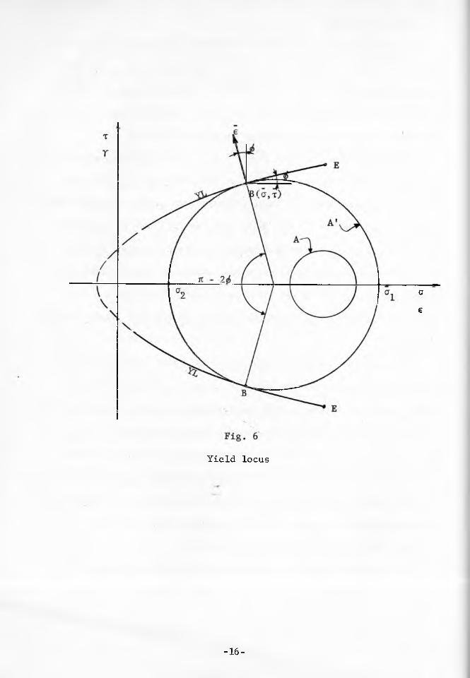
The properties of a yield locus, Fig. 6 , will now be discussed in
some detail. 1 The stresses acting in a cross-section of a solid are
described by a stress vector whose component are: the normal pressure
a and the shear stress t. The yield locus is the locus of the values
of (ct,t) at which permanent deformation, or yield, occurs. In plast
icity, the equations of equilibrium are assumed satisfied, therefore,
the stresses described by the yield locus cannot be exceeded. This
implies that the yield locus is the envelope of the Mohr stress circles
at yield.
For any stress condition represented by a Mohr circle A, not
touching the yield locus, the solid is rigid (or elastic). When the
stress condition changes so that the corresponding Mohr circle A' comes
in contact with the yield locus, yield stresses, described by the
points B, develop in the two planes of the solid inclined at angles -j- _-(#,/4 - i/2) to the direction of the major pressure G , and the solid
deforms. These two planes are called the slipplanes, and are represent
ed by two slip lines in the principal, physical plane x-y, Fig. 7.
Angle i is the angle of friction of the.solid.
The strain rate which accompanies a yield stress is described by
-15-
a
e
Yield locus
-16-
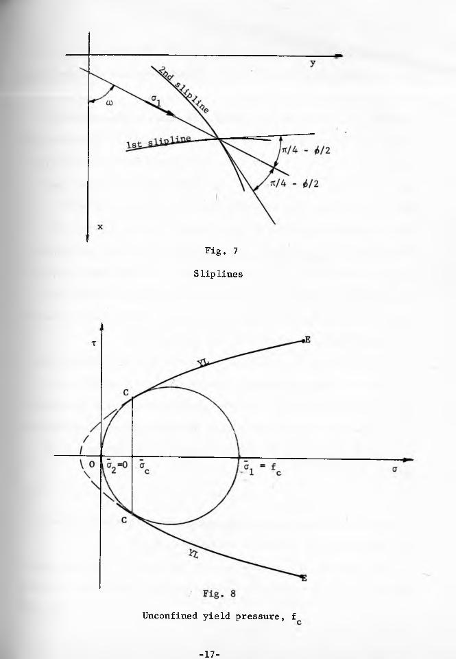
Fig. 7
Sliplines
Unconfined yield pressure, f
-17-
the strain rate vector e, whose components are: the normal strain rate
e and the shear strain rate y„ If the coordinates (e,Y) are superimposed
over the coordinates (o,t), Figures 5 and 6 , then by the principle of
normality [?], the strain rate vector e is normal to the yield locus
at the point of contact with the Mohr stress circle. It is evident from
Fig. 6 that any point of contact, B, enforces a direction of the strain
rate vector which contains a negative, hence expansive, normal compo
nent of strain rate and, therefore, implies dilation of the solid.
The only exception is point E, the terminus of the yield locus, at
which normality only restricts the direction of the strain rate vector
to within a sector <t>, - ff/2, shown in Fig. 5. When the Mohr circle is
tangential to the yield locus at point E, normality allows the solid
either to dilate, or to contract, or to deform without change of density.
This is the condition which occurs during steady flow.
It is observed that the angle, of friction <£> is not constant along
the yield locus but varies from a minimum at points E to Jt/2 at the
intercept with the cr-axis. The shape of the yield locus at low values
of a is important in this work because it affects the value of the major
pressure f which causes failure at a traction free surface. f is,»< ....... c cdefined thus
°2 ~ O’ CT1 = fc”
f is called the unconfined yield pressure and is obtained by inscrib
ing a Mohr yield circle through the origin 0, Fig. 8 .
The curvature of the yield locus at low values of a is not generally
recognized and lacking complete experimental verification, the following
-18-
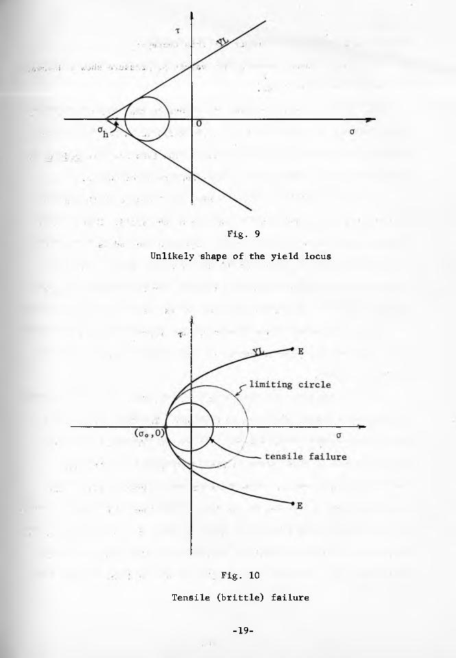
Fig. 9
Unlikely shape of the yield locus
Fig. 10
Tensile (brittle) failure
-19-
arguments are offered in support of this concept:
(a) Direct shear tests at low values of pressure show a downward
curving of the yield locus.
(b) If the yield locus were to intersect the a-axis at an angle
other than »/2, as shown in Fig. 9, the solid would be stable under a
hydrostatic tension but would fail if the tensions were reduced to
those given by the Mohr circle. This appears unreasonable.
(c) The yield locus shown in Fig. 10 allows for both, tensile
(brittle) failure, and shearing failure of the solid. Namely, there
exists a limiting circle of a radius equal to the radius of curvature
of the yield locus at point (ao,0) such that all stress conditions
represented by circles within the limiting circle approach the yield
locus at point (ao,0), where the shear stress is zero, causing failure
in tension; all other stress conditions are represented by Mohr circles
which approach the yield locus at non-zero values of shear, causing
failure in shear.
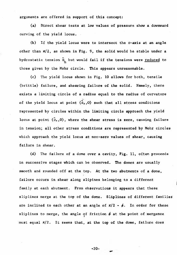
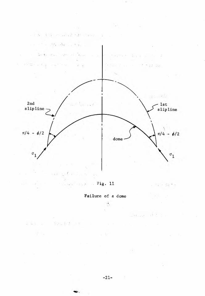
(d) The failure of a dome over a cavity, Fig. 11, often proceeds
in successive stages which can be observed. The domes are usually
smooth and rounded off at the top. At the two abutments of a dome,
failure occurs in shear along slipines belonging to a different
family at each abutment. From observations it appears that these
sliplines merge at the top of the dome. Sliplines of different families
are inclined to each other at an angle of jt/2 - tfS. In order for these
sliplines to merge, the angle of friction at the point of mergence
must equal a/2. It seems that, at the top of the dome, failure does
-20-
. Fig. 11
Failure of a dome
-21-
occur in tension, and = *t/2 .
It is evident that an accurate determination of the value of the
yield locus at point C, Fig. 8 , is necessary to obtain a reliable value
of f£. A linear extrapolation of the yield locus from test values
obtained at pressures considerably higher than C would give erroneous
results.
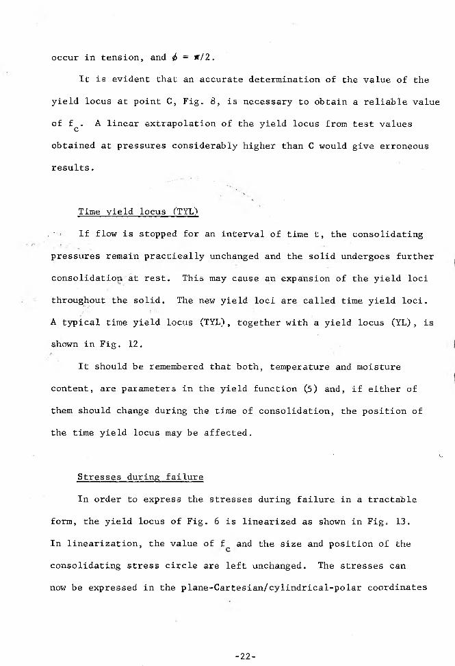
Time yield locus (TYL)
.• j If flow is stopped for an interval of time t, the consolidating
pressures remain practically unchanged and the solid undergoes further
consolidation at rest. This may cause an expansion of the yield loci
throughout the solid. The new yield loci are called time yield loci.
A typical time yield locus (TYL), together with a yield locus (YL), is
shown in Fig. 12.
It should be remembered that both, temperature and moisture
content, are parameters in the yield function (5 ) and, if either of
them should change during the time of consolidation, the position of
the time yield locus may be affected.
■ - ' I
Stresses during failure
In order to express the stresses during failure in a tractable
form, the yield locus of Fig. 6 is linearized as shown in Fig. 13.
In linearization, the value of f and the size and position of the
consolidating stress circle are left unchanged. The stresses can
now be expressed in the plane-Cartesian/cylindrical-polar coordinates
-22-
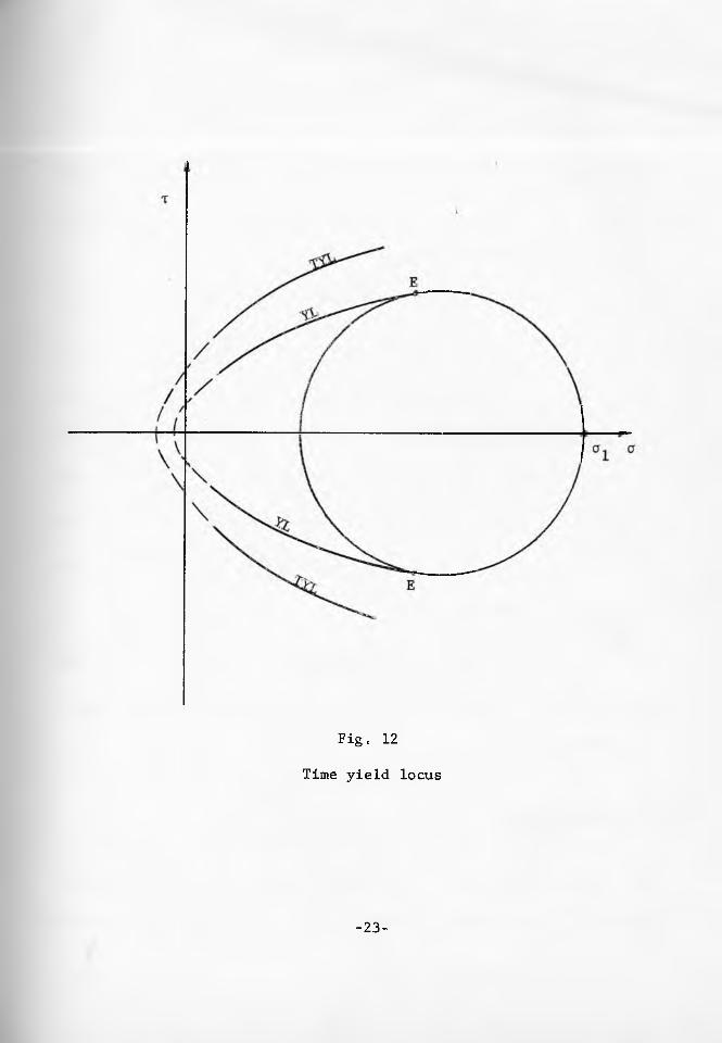
Fig. 12
Time yield locus
-23-

by
a = a(l + sin cos 2cu) - f ^ s'i'- (29)x c 2 sin p
- . / n \ „ 1 - s in ^a = o(l - sin <b cos 2d>) - f — — — — 7 , y c 2 s m p (30)
T = cr sin & sin 2co; (31)xy ’and in the polar/spherical coordinates, by
a = a(l + sin i cos 2\|/) - f —r^~p, (32)r c 2 s m p
*= a(l - sin & cos 2t) ~ f — sin-7 (33)y c /. s m p
t ■- cr sin sin 2ilr. (34)r0
The principal pressures are
an = a(l + sin $>) - f — — Sin ~, (35)1 c 2 sin 0
a = a(l - sin ) - f -- (36)Z c Z a in p
cr = afl + k sin - f — -— (37) O! ' c 2 s m p
In the above equations
- J 1 °2 . 1 - sin <t> . .0 = —— — — + f -----7— 1 , (38)2 c 2 s m p
and k = + 1 for converging failure, and k = - 1 for diverging failure,
the same as for flow.
Flow-function
The concept of the flow-function is introduced as a measure of
the flowability of solids. This concept is obtained by substituting
relation (6) for y in eq. (5), and by placing the minor yield pressure
-24-
Fig. 13
Linearized yield locus
-25-
a2 ~ 0. The corresponding value of the major pressure is the unconfined
yield pressure f , eq. (28). Eq„ (5) then assumed the form
fc = G(cr1 ,t,T,H), (39)
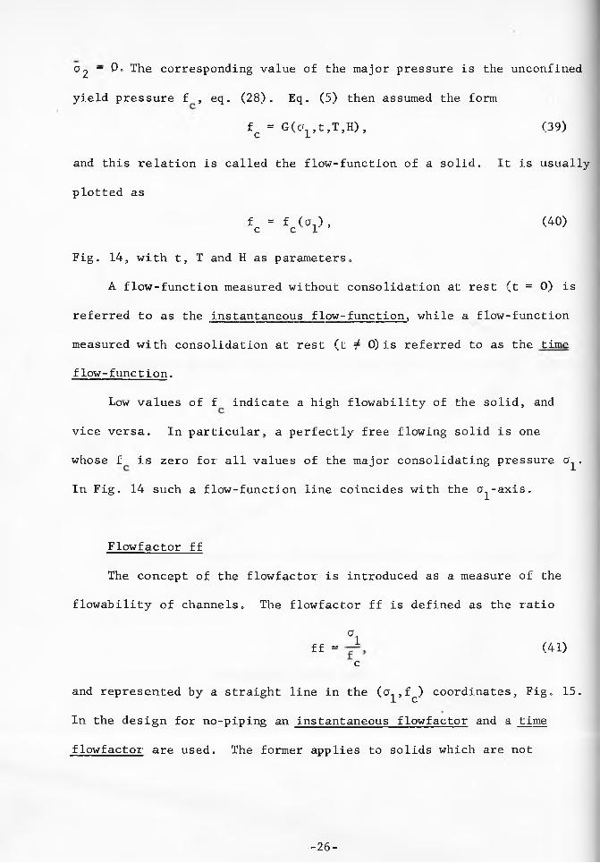
and this relation is called the flow-function of a solid. It is usually
plotted as
* C - W - <40)
Fig. 14, with t., T and H as parameters.
A flow-function measured without consolidation at rest (t = 0) is
referred to as the instantaneous flow-function, while a flow-function
measured with consolidation at rest (t i- 0) is referred to as the time
flow-function.
Low values of f indicate a high flowability of the solid, and
vice versa. In particular, a perfectly free flowing solid is one
whose f is zero for all values of the major consolidating pressure cr.
In Fig. 14 such a flow-function line coincides with the cr -axis.
Flowfactor ff
The concept of the flowfactor is introduced as a measure of the
flowability of channels. The flowfactor ff is defined as the ratio
a!ff = (41)
c
and represented by a straight line in the (a^,fc) coordinates, Fig. 15.
In the design for no-piping an instantaneous flowfactor and a time
flowfactor are used. The former applies to solids which are not
-26-
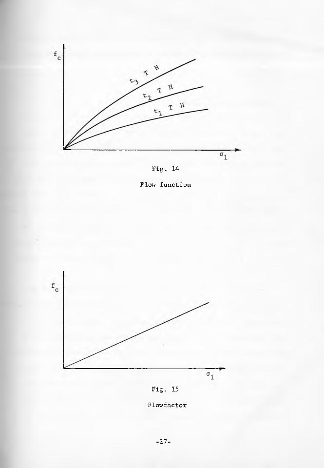
Fig. 14
Flow-function
Fig. 15
Flowfactor
-27-

affected by consolidation at rest, while the latter applies to those
whose time flow-function exceeds the instantaneous flow-function by,
say, 20%.
Wall yield locus (WYL)
A side boundary between a region in a plastic state of stress
and a rigid (or elastic) stationary region is called a wall. In gen
eral, there is a velocity discontinuity along a wall, the wall frictional
strength is fully mobilized, and the stresses acting on the wall lie
on a wall yield locus, which is represented by a line WYL in the (ct,t)
coordinates, Fig. 16. Since the solid is in a plastic state, the stresses
at the wall lie at one of the points of intersection W of the wall yield
locus with a Mohr stress circle tangential to the yield locus of the
solid,Y'L. During flow, the circle is tangential to the yield locus at
the points E and is also tangential to the effective yield locus (not
shown in Fig. 16).
The position of the wall yield locus depends on the frictional
conditions at the wall. These conditions may range from perfectly smooth
(in concept, at least) to the full strength of the flowing solid. In
the former case, the wall yield locus is represented by the positive
part of the cr-axis, the stresses at the wall are defined by one of the
points M, and the wall can transfer no shear stress. In the latter
case, the wall yield locus merges with the yield locus of the solid
and the stresses at the walls are given by one of the points E (or
points B in incipient failure)„ Such a wall will be referred to as a

I iT
Fig, 16
Wall yield locus
-29-

"rough wall". A rough wall is a slip line.
The wall yield locus shown by line WYL in Fig. 16 denotes a degree
of weakness of the wall as compared to a rough wall and such a wall
will be referred to as a "weak wall".
In this work, the stresses at the walls assume values which lie on
the arc E'ME", hence the stresses at a weak wall are represented
either by point W' or W"„
Observations of flow patterns in models and measurements of wall
yield loci indicate that the introduction of a wall made of an extran
eous material, even a coarse material, causes a significant drop in the
cohesive and frictional forces at the wall. There seems to be no
practical way of gradually decreasing the weakness of a wall by, say,
increasing its coarseness until the wall yield locus merges with the
yield locus of the solid. Experiments indicate that for weak walls
the points W locate within the arc T'MT" of the Mohr stress circle,
and that the wall yield locus can be linearized without a significant
loss of accuracy. Since linearization reduces the amount of testing
necessary to define the wall yield locus, and greatly simplifies
the analysis, it will be adopted in this work. The position of a
wall yield locus becomes thus fully determined by the magnitude of
the angle of friction £$' between a solid and a wall.
In plane strain the channel may be asymmetric and the frictional
conditions at each wall may be different, as shown in Fig. 17. In
this case, the relations have to be developed separately for each wall.
The values relating to a point of a wall inclined at angle 9' to the
-30-
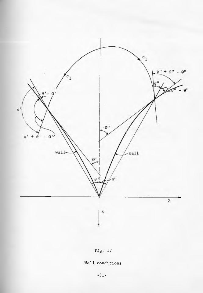
Fig. 17
Wall conditions
-31-

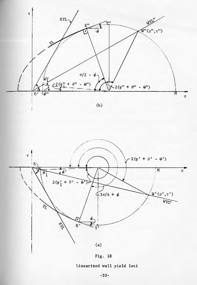
x-axis are denoted by primes. The corresponding part of the Mohr stress
circle and the yield loci are shown in Fig. 18 (a), the wall yield locus
is determined by the angle of friction The relation between the
stresses at the wall are
^ 7 = tan <i>' . (42)
From the geometry of the Mohr circle it follows that
sin[2(\|r" + 0' - 0 ’) - - Jt] = ,8 in o
and the significant solution for \|r' is
+ 0 ' _ Q« = £ + h p + Arc sin - - “ ) , (43)2. Z s in o
For rough walls, point W' merges with point. E' and it is evident from
Fig. 18 (a) that
\|r1 + 9 ' ~ 0 ’ = "Tit + (44)
or, noting that it is the period of angle \|r' , eq. (44) can also be
written a|t 1 + 6 1 - 0' = - it/4 + i/Z.
Similarly, the values relating to the wall inclined at angle -0"
to the x-axis are denoted by double-primes, and the corresponding part
of the Mohr stress circle and the yield loci are shown in Fig. 18 (b).
The wall yield locus is located by the angle of friction between
the solid and the wall. Relations (42) to (44) now become
• 77 = tan <6" (45)
+ 0" . 0" = £ _ + Arc sin 4 S-^) , (46)l I s m o
-32-
T
Linearized wall yield loci
-33-
PART II
STEADY STATE FLOW
General equations
In this section the differential equations required for the
solution of the stress and velocity fields in steady state flow are
presented. The adopted yield function allows the stress equations to
be uncoupled from the velocity equations and to be solved first. The
solution of the stress field produces the direction of the major
pressure to(x,y) and the value of density T(x,y) throughout the field,
and suitable velocity fields can then be computed.
The boundary conditions have to be satisfied in both, the stress
and velocity fields and certain physical conditions imposed on the
stress and velocity fields have to be. met.
All the differential equations are hyperbolic and each field
requires the solution of a set of two partial differential equations
of first order. The equations are presented in a form suitable for
numberical calculations by the method of characteristics.
Stress field„
In the plane-Cartesian/cylindrical-polar coordinates x, y, 01,
Fig. 2, the equations of equilibrium are
-35-

These two equations together with the equation of the effective yield
locus (11) and the empirical relation for density (26) can be solved
for the four dependent variables (a , cr , t ,T) in plane strain. r ■ x y xyIn axial symmetry, the fifth dependent variable $ is taken care of
by the additional equation (22).
The equations of equilibrium are first expressed in terms of a
and 03 by means of equations (14) - (16) and (22), thusfj n n "T ('y | (1 + sin 5 cos 2cd)~ + sin 5 sin 2cu - 2 ® sin 8 sin 2o> +x y x
- 8 cr+ 7.0 sin 8 cos 2ca = y0(l + cr)- - m — sin 8 sin 2cd,
sin 8 sin 2cd + (1 sin 8 cos 2to) + 2 0 sin 8 cos 2o) + dx • ay ox
■ + 2o sin 8 sin 2cd = m ~ sin 8 (k + cos 2ao) .
Now the following abbreviation is introduced [15]
S = In (50) Oo
where a0 is an arbitrary constant. The differential equations then
reduce to the following form

where
/-i , , S\ / , 5N , , , it , 8.To (1 + o) s m ( a ) - + —) c o s (a ) + - - —) + k c o s (a ) -A = - ' ' — r--1- m —-- ------ - ’
2 a s i n 5 cos(oc> + - —) 2y cos(cd + — - —)
To ( 1 + cr)^sin(o) + -r - ~ ) cos(co - y + tj) + k cos(cd + 7 - § )
B -----------------— V - V - m ------- -— ------ 7 5 — L • <52>2o s m 8 cos(co - ^ + —) 2y cos(a) - — + —)
In the first characteristic direction,
dx = tan(“ + 4 “ 2^’ 53)
the left hand side of eq.(a) is a total derivative
= A. (54)d (S + co)dx
Similarly, in the second characteristic direction,
S = t 3 n ( “ " I + 2} 5 (55 )
the left hand side of eq.(b) is a total derivative
d<s : m> - B. (56)CIX
It will be observed that the two stress characteristics inter
sect at an angle it/2 - 8 , and form angles + (^/4 - 8/2) with the
direction of the major pressure.
Velocity field.
The velocity field is computed with the assumption of continuity
and isotropy. The equation, of continuity in steady flow can be
-37-

written as follows
I-(r u ym) + |^(r v ym) - 0, (57)
where u and v are the components of the velocity vector in the direc
tions of the coordinate axes x and y, respectively, Fig. 19. Density
T is eliminated by means of eq. (26), yielding
[ ( 1 + cr) uym] + [ ( 1 + a)^vym] = o,
which expands into
where
v , f3 ,dcr . da e = m ---r T~r~<.>n u t -5—y 1+ a o x ay+ rg-gZ u + v) . (59)
The principle of isotropy states that the directions of the
principal strain rates coincide with the directions of the principal
stresses. The normal, compressive strain rates and e , and the
shear strain rate T a r e expressed in terms of the velocity com
ponents as follows
C>U c * v cH l S v ,,
Ex ■ ' X " ey ’ - 3 F- Txy = ■ Ty ' S ’ (60)
The equation of isotropy then can be written
du _j_ dvtan 20) = |2— (61)
cSx By
In order to find the characteristic directions and the relations
-38-
which hold along the characteristics, equations (58) and (61), together
with the equations of the total derivatives
dx + dy = du, ^ dx + dy = dv,
are solved for du/dx to yield
3u dy + + e(fe - tan 2a,) . (c)a x " ' dx [ £ - ta„(a, + f>] [ £ . t - O - f ) ]
The characteristic directions are
= tan(d) + -|) . (62)
Hence, the velocity characteristics are orthogonal and do not coincide
with the stress characteristics.
In the directions of the characteristics, the numerator of eq.(c)
is zero and, with the substitution of the appropriate expression (62)
for dy/dx, reduces to
= (63)dy dx cos 2co
In both equations (62) and (63) the top sign applies along the first
characteristic and the bottom sign along the second characteristic.
Sometimes it is more convenient to have the velocity vector
expressed in terms of its projections v^ and v2, Fig. 19, on the
directions of the characteristics. A substitution for
u = - v^ sin(co - it/4) + v^ sin(oo + fl/4),(64)
v = v^ cos(o) - rt/4) - v^ cos (od + it/4)
in eq.(63) leads to the following relations:
-39-

along the 1st. characteristic: = tan (co + -) , ' . (65)
dv., dcu m dy ft da ft da
+ V2 + 2? <V1 + V2 + TTCf^I W x + 2W) ‘ ° ’ (66>
In the above equations, as well as in the two equations below, the
derivatives are taken in the direction of the 1st or the 2nd character
istic as indicated by the subscript.
Along the 2nd characteristic: “ tan (co - —■) , (672
dv d.co m dy 6 v.. da ft v~a — " v i ~a — ' + T~ v i 1 — + v 0 ) - ~/ i. a ~— + T T Tw T ~ r ~ ~ ° * (68dy^ 1 dy^ 2y 1 dx^ 2 2^1+u) dx^ 2(1+a) dy^
Superposition. Since both., the equation of continuity (58) and of
isotropy (61), are linear and homogeneous, a linear combination of two
(or more) solutions of a velocity field is also a solution. This
property of the velocity field is very convenient in the development
of physical solutions„
Physical conditions
The following conditions are imposed on the stress and velocity fields
on physical grounds: -
A. Stresses are positive (tension not allowed) and bounded.
B. Along a line of infinite shear strain rate, frictional and cohesive
forces are fully mobilized. This implies that stresses along such a
line lie either on the yield locus or on the wall yield locus, hence,
such a line, is either a slip line or a weak wall.
-40-
----- i**y, v
X , u
Fig. 19
Projections of the velocity vector
on the characteristic directions
-41-

C. The velocity V of an element of a solid is bounded.
D„ The acceleration of an element,
dV dV - . v2 - ....’ d£ S + T " <69)
S
along the path of its travel, Fig. 20, is bounded. This implies that
dV/dt is bounded everywhere, and 1/p is bounded everywhere with the* S .
exception of points at which V = 0.
E. Singularities in density are inadmissible.
Grids, special lines and regions
The solution of a stress field defines the function
cd = co(x,y) , (70)
where tan co = dy/dx is the direction of the major pressure Eq.(70)
thus is the differentia 1 equation of a grid of lines of action of
pressure o , Fig. 21. While the solution of flow does not require the
determination of this grid, eq.(70) is used to locate the following
grids, special lines and regions.
1. Stress characteristics. The slope of the stress characteristics,
Fig. 22, is given by
cd t (jt/4 - 8/2) . (71)
The fields shown in Figures 22 to 24 assume that the walls are rough.
2. Velocity characteristics. The slope of these lines, Fig. 23, is
cut */4. * (72)
It will be ovserved that the velocity characteristics form two bunches
whose stalks are located at the vertex of the channel. The stalks are
-42-
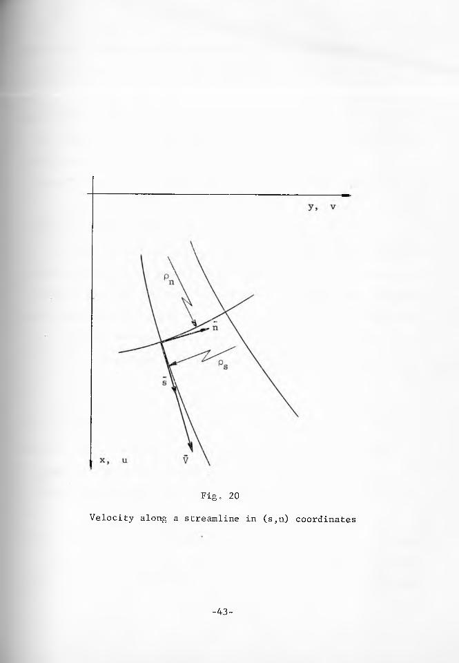
Fig. 20
Velocity along a streamline in (s,n) coordinates
-43-
within the walls of the channel because the walls are rough. The stresses
at the walls are given by the points E, Fig. 18. If the walls were weak
in such a degree that the stresses at the walls were given by the points
T (T = W ) , Fig. 18, then the wall on each side of the channel would aline
with a velocity characteristic. The stalks would be at the walls. If
the walls were weaker yet, so that the stresses at the walls were given
by the points W, as shown in Fig. 18, the stalks of the velocity chara
cteristics would be cut off by the walls.
3. Lines of maximum shear strain rate. These lines are inclined
at angles "t rt/4 to the lines of the principal strain rates and, with
the assumption of isotropy, also to the lines of the principal stresses.
Therefore, the slope, of these lines is 0) "t it/4 and they coincide with
the velocity characteristics, Fig. 23. The lines of maximum shear strain
rate are important because some of them can be observed through a
transparent wall of a model and thus provide an experimental check of
the analysis.
4. Slip lines. Under conditions of flow, the slip lines, Fig. 24,
do not coincide with either the stress or the velocity characteristics.
However, slip lines are significant because by the physical condition
B a line of infinite shear strain rate across a solid can occur only
along a slipline. A slipline has the slope of either of the two angles
co t (it/4 - 412). (73)
From Fig. 24, it is evident that the sliplines, like the velocity charac
teristics, form two bunches with stalks at the vertex of the channel.
Since the walls are rough, they aline with the sliplines and, therefore,
-44-
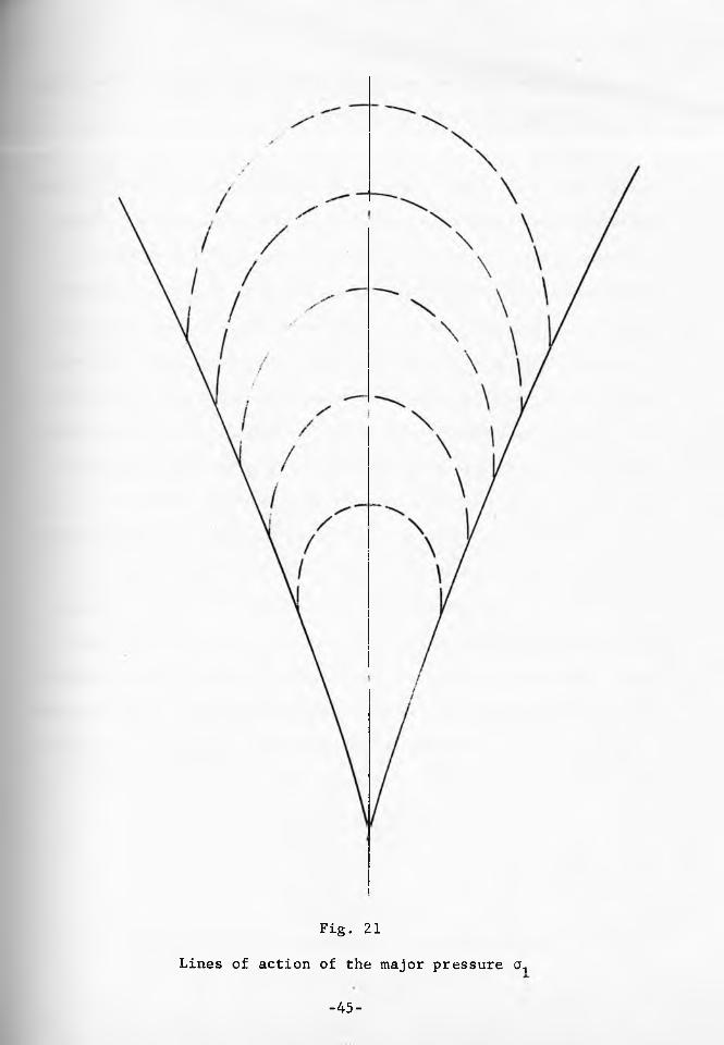
Fig. 2.1
Lines of action of the major pressure an
-45-
the stalks of the sliplines are at the walls. Any weakness at the walls
would cut off the stalks of the sliplines*
, During flow, angle ^ is measured at the points E of the Mohr stress
circle, Fig. 5, At these points angle ^ is always smaller than 5; this
follows from the condition of convexity of the yield locus [7]. Angle
<i> is also greater than zero;; this can be demonstrated by means of
models in which the lines of maximum shear strain rate can be observed
through a transparent front wall. If 6 were zero, then e q , (73) would
be identical with eq,(72) and, in a channel with tough walls, the walls
would coincide with the lines of maximum shear strain rate. The stalks
of the latter lines would lie at the walls while, in fact, these stalks
are observed in the positions shown in Fig. 23, Another illustration
of <i> > 0 is provided in the section "Flow in vertical channels",
5, Streamlines, In steady state flow the paths of flowing elements
of the solid are independent of time and are called streamlines.
Streamlines have the following two properties" they cannot have
cusps, (except at points where V = 0), and they cannot intersect each
other. The former follows from the physical condition D which requires
that 1/ pg be bounded. The latter is demonstrated from the consideration
of the equation of continuity in the orthogonal, curvilinear coordinates
(s,n), Fig, 20, This equation is of the form
S(r V pn ym )
• ^ = 0,
and it follows that
T V p ym = f (n) ,. n
It is easy to show that at the intersection of two streamlines p 0,
-46-

Fig. 22
Stress Characteristics
-47-
hence V-?*°°, which is not permitted by the physical condition C „
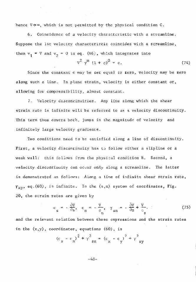
6. Coincidence of a velocity characteristic with a streamline.
Suppose the 1st velocity characteristic coincides with a streamline,
then Vj = V and v^ - 0 in e q . (66), which integrates into
V2 ym (1 + a)P = c. (74)
Since the constant c may be set equal to zero, velocity may be zero
along such a line. In plane strain, velocity is either constant or,
allowing for compressibility, almost constant.
. 7. Velocity discontinuities. Any line along which the shear
strain rate, is infinite will be referred to as a velocity discontinuity.
This term thus covers both, jumps in the magnitude of velocity and
infinitely large velocity gradients.
Two conditions need to be satisfied along a line of discontinuity.
First, a velocity discontinuity has to fallow either a slipline or a
weak wall:' this follows from the physical condition B. Second, a
velocity discontinuity can occur only along a streamline. The latter
is demonstrated as follows: Along a line of infinite shear strain rate,
T*xy» ecl*(60), is infinite. In the (s,n) system of coordinates, Fig.
20, the strain rates are given by
&V V dv . V . , -ve = - XT, e = - , r = " x : + (75‘)s n P sn °n. p .
n s
and the relevant relation between these expressions and the strain rates
in the (x,y), coordinates, equations (60), is
j 2 2 2 (e - e ) ' + r = (e - e ) + r
s n sn x y xy
-48-

Fig. 23
Velocity characteristics
-49-
In this equation
dV _ SV dn dV SV _ dt dn dt dt 3s _ds “ v ’
dt
since ds/dt = V and dn/dt a 0. All the terms on the left hand side of
eq.(d) with the exception of dV/cki are bounded by the physical conditions
C and D. Hence, along a line of velocity discontinuity, it is necessary
that SV/Sn»»5 which means that a velocity discontinuity follows a
streamline.
A velocity discontinuity, though it is a line of infinite shear
strain rate, does not, in general, coincide with a line of maximum
shear strain rate; the latter strain rate being bounded. A velocity
discontinuity separates two regions which may be both plastic, both
rigid (or elastic), or one plastic and the other rigid (or elastic).
A velocity discontinuity often originates at the top boundary of
a channel. In channels with rough walls all the slip lines enter the
stalks at the vertex, and discontinuities can extend from the top to the
bottom of the channel. In all practical channels with weak walls the
walls cut off the stalks of the slip lines. A velocity discontinuity
cannot continue to an intersection with a wall, since that would involve
an intersection of the streamline, which coincides with the discontinuity,
with the walljwhich itself is a streamline. A velocity discontinuity
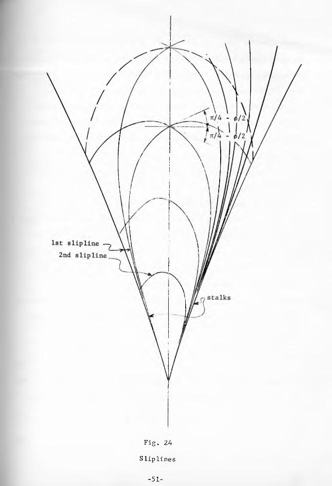
Fig. 24
Slip lines
-51-
cannot transfer from a slipline of one family to another slipline of
the other family because that would imply a cusp in the streamline at
the transfer point. In channels with weak walls a velocity discontinuity
which originates at the top boundary dampens out within the field.
8. A straight velocity characteristic in incompressible plane
Strain. Suppose that in plane strain a first1velocity characteristic
is straight and the solid is incompressible, it then follows from eq.
(66) that v^ is constant along that characteristic.
. 9. Walls. A wall separates a plastic region from a stationary
rigid (or elastic) region.
Usually, there is a velocity discontinuity along a wall. The
wall then coincides with a streamline, and stresses along the wall are
defined by either the yield locus or the wall yield locus. When the
solid flows within rough walls, the walls coincide with sliplines and
the stalks of the bunches of sliplines intersect the lower boundary
of the channel. Therefore, any slipline which intersects the top
boundary of the channel may form a wall. In consequence, the walls can
shift readily in the upper part of the channel, adjusting to the top
boundary conditions.
In accordance with eq„(3), at the walls, Fig. 17, there is
\|/' + 0' - 0)' and f" + 0" - co". (76)
For rough walls t' and V are eliminated by means of equations (44) and
(47) leading to the following expressions for the slopes of the walls

It will be noted that, since it is the period of angle co, eq.(77)
can also be written 0' = oo1 + Jt/4 - i/2.
When the solid flows within weak walls, the slopes of the walls are
found from expressions (43) and (46) with appropriate substitutions of
(76), thus
For straight walls intersecting at the origin, 6' = O ' and 6" = 0".
When a velocity characteristic coincides with a wall along which
there is a velocity discontinuity, the wall is weak to such a degree
that the wall yield locus passes through the point T of the Mohr circle.
For the linearized wall yield locus, Fig. 18 (a), this implies
In this case, the velocity discontinuity also coincides with a streamline
and that enforces the restriction on the magnitude of the velocity along
the wall expressed by eq.(74).
When there is no velocity discontinuity along a wall, the wall
need not be a streamline and the stresses along the wall need not lie
on a yield locus or on a wall yield locus. If such a wall coincides
with a velocity characteristic then the velocity boundaries at the top
and at the bottom of the channel have to be continuous at the w a l l s .
In practice, this is seldom attained and these conditions lead to non
steady flow. This is prevalent in axi-symmetric flow within rough walls.
If such a wall does not coincide with a velocity characteristic then a
(79)
q" = co" . [-2 _ h i " + Arc sin S i n 'f ) ] .2 2 s in o
(80)
tan i ' = sin 6. (81)
-53-

zero velocity region is enforced. This is discussed below.
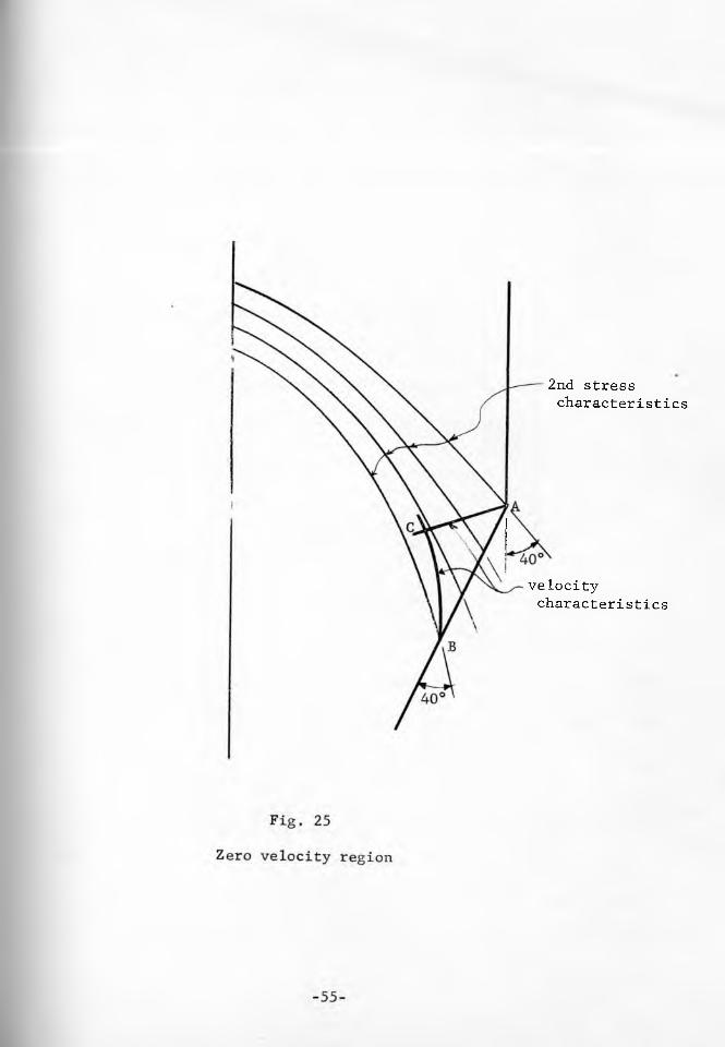
10. Zero velocity regions within a plastic field. This concept
is very useful in the development of fields in channels with sharp
changes in cross-section, as shown in Fig. 25, because it allows the
use of a continuous stress field. The stress characteristics of the 2nd
family have to intersect the wall at an angle of 40° (in this example) i
to satisfy the wall yield locus and allow a velocity discontinuity along
the wall. The stress characteristics above point A and below point
B do so satisfy the WYL, Between the points A and B, the stress char
acteristics bend in gradually and the stresses at the wall are below
yield values, hence no velocity discontinuity can o:cur along A B .
Since AB is not a velocity characteristic, zero velocity along AB
enforces a zero velocity region ABC where C is the intersection of
two velocity characteristics (heavy lines) through A and B, respectively.
Since, further, there can be no velocity discontinuity along the line
ACB (not a slip line) that line is not a streamline. Streamlines develop
smoothly around ACB. Zero velocity regions can be observed in a
model with a transparent wall. Indeed, it was from observations of
models that this concept arose.
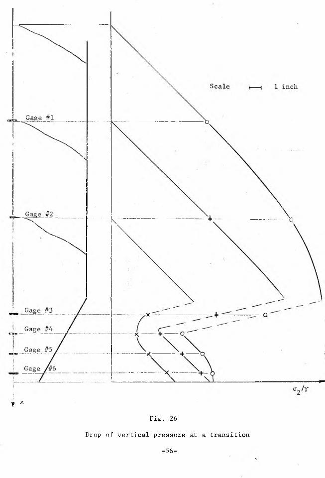
In a bin, zero velocity regions occur at the transition from the
vertical portion to the hopper. They have the effect of narrowing down
the channel at the transition and explain the drop of the vertical
pressure along the axis of symmetry. This drop was measured by the
author several years ago, Fig, 26, and was reported in references
[16, 17].
-54-
2nd stress
characteristics
velocity
characteristics
f x
Fig. 26
Drop of vertical pressure at a transition
-56-
11. Stress discontinuities may occur only along streamlines.
This follows from the fact that all real materials are compressible,
and a discontinuity in stress implies a discontinuity in density. An
element of solid flowing across a stress discontinuity would undergo
a discontinuity of density and, therefore, an infinite acceleration,
which is contrary to the physical condition D. Since the lines along
which stress discontinuities might be expected to arise usually cross
the streamline field, the existence of discontinuities is unlikely.
12. Stress singularities are inadmissible, because they would
imply singularities in density which in a real solid are not acceptable
by the physical condition E.
Converging channels
Equations of stress
In this section it will be advantageous to use the polar/spherical
coordinates r, 0, OC. The equations of equilibrium in these coordinates
are
da , S t „
H----- nT"-- 1---[o - oa + m(a - a r/) + m t a cot 0] +or r o0 r r 0 r OC' r 0
+ T cos 0 = 0 , (82)
dr— + r ~ dd + 7 [m^a0 " U0t) cct 6 + (2 + m ^Tr0J - T sin 0 = 0.(83)
These equations are now transformed as follows: first, expressions
(17), (18), (19) and (20) (with k = +1), and their appropriate deriva
tives are substituted for the component stresses; second, the substitution
-57-
o-=rr(r,e) s(r,0) . (84)
is made; third, the derivatives ds/d© and ds/c)r are separated, leading
to the two equations „
ds+ s f(r,0) + g(r,0) = 0, (85)
r ^ + s h(r,0) + j(r,0) = 0 , ' (86)
where
f(r,0) = 2 ( ^ + l)-2^” ^ sin 2^ + 2r ^ -S:Ll --(sin 5 + cos 2f) +cos 5 cos S
+ — + m -^— "(1 + sin 8) [sin 2\(r - cot 0 ( 1 + cos 2\|/) ], (8/^ cos
, sin 6 . .... , „, N sin 0 /r>n\g ( r ,0) = - --- s m ^0 -t 2\|/) - ------- — , (88)
cos 5 cos &
h(r,g) = 1 + 2(^g + 1) ™ - ^ ~ ( c o s 2^ - sin &) - 2r ^ S^n ^ + |cos S cos 8 I
+ ~ + m (1 + sin 8) (cot. 0 sin 2\|r + cos 2\|r - 1) , (89)T cos &
j (r ,0) = - ™ 1-n“2_5, cos(0 + 2\(r) + (90)cos 5 cos 8
The converging channels under consideration will be assumed to
possess a vertex at which the extensions of the walls intersect. It
will be shown that, with some continuity conditions satisfied, stress
fields in all converging channels, irrespective of their top boundary |
and walls away from the vertex, approach a unique and relatively simple
stress field at the vertex. That unique stress field will be called
the "radial stress field',1 because it is the stress field compatible
with a radial velocity field. The radial stress field is fully defined
by the slopes of the tangents to the walls at the vertex (S', -0") and
I
-58-
4
the physical parameters of the solid and the walls (6,g$',^").
While a physical channel can never be brought to a vertex,
it is expected that the radial stress field is closely approached
within a substantial region of the vertex, a region which will usually
include the outlet of the channel. Since the knowledge of the stress
field at the outlet of the channel is required in the derivation of
flow criteria, the uniqueness and the simplicity of the radial stress
field are of a great, advantage in this derivation.
In the considerations which follow the origin of the coordin
ates will be located at the vertex of the channel.
f '
Radial stress field.
Derivation. If it is assumed that
t = K e ) (91)
and
Y = const. (92)
Then the coefficients of the equations (85) and (86) assume the sim
plified form
f(6) = 2(^- + 1) —— sin 2\|r + cos 5
+ m (1 + sin S)[ sin 2\j/ - cot 6(1 + cos 2 r)] , (93)cos 6
sin 6 . , „,x sin 6 ,„,sg (6) = - --- 2” sin(0 + 2^) - --- (94)
cos S cos 5
-59-
h(0) = 1 + 2(~^ + 1) S,:i'n0'~ (cos 2\|r - sin &) +O.C7
cos o
+ m S'*‘n2^(1 + sin 8) (cot & sin 2^ + cos 2\jr - 1) , (95)cos 6 .
j(6) = - ~ - n-2- cos(0 + 2\|r) + -°-^e-. (96)cos 5 cos 5
Equations (85) and (86) now become
£ + s f(0) + g (0) = 0, (a)
r | + s h(0) + j(0) = 0, (b)
and integrate into
. -/f(0)d0 -/f(0)d0 / f(0)d0s = c(r) e - e /g(0) e d0,
s = k(0) r"h - s r h ( 0 ) .
Hence
(c)
. . -/f(0)d0 /f(0)d0
= e /g(0) e , (d)
and there are two alternatives: either
k(0) ~ c(r) = 0, (e)
or
~/f(0)d0k(0) = e , and c(r) = r .
Consider the latter case. Evidently h = const. ^ 0. Eq. (d)
is differentiated, thus
g(0) h = f(0) j(0) + (f)
Now differentiation of eq.(96) yields
-60-
In this equation and in eq. (93), the derivative d\|//d0 is eliminated
by means of eq.(95) to yield
These expressions and expressions (94) and (96) are now substitut
ed for the appropriate functions in eq.(f), which after transformations
becomes
In plane strain h = 1 and eq.(95) yields d\|r/d0 = -1. This implies
an elementary field with rectilinear characteristics, which enforce a
constant velocity throughout the channel. This does not provide a
solution to converging flow.
In axial symmetry, it follows from eq.(95) that, at the axis, for
0 = 0, \jr equals either 0 or rt/2. Any other value would enforce d\|//d0 =
at the axis, and that is inadmissible since it would imply an unbounded
strain rate. Consider the initial condition 0 = 0, \)r = tc/2. For these
values, the numerator and denominator of e q . (g) vanish and the limit i
_ 9dj _ sin(0 + 2^) |(h - l)cos 5 - sin 5(cos 2\|i - sin 5)1 sin 0 d0 ~ 2C , ' 2*
cos 6(cos 2\||r - sin 6) cos 6
msin S(1 + sin 5) sin (0 + 2\[/) (cot 0 sin 2\|/ + cos 2\|r - 1)
2cos 6 (cos 2\|r - sin 6)
and
sin 5[sin 2^ - cot 0(1 + cos 2^)] cos 2t - sin 6
oh = 1 + m £ sin S[cos 2i|f + cos 2(0 + 2\|f) ] - sin (0 + 2\|r) +
t) r\- cos 2(0 + \|/) - cos 0 j- /cos 5 [cos 2(0 + i|/) - cos 2i|f], (g)

established by twice applying l'Hospital's rule, yielding
h . , , M n S 31(^ )012 * 4(^ )0+ 1* 1 + sin 6 2(i i }o + x ’
dC7
2 2because, from eq,(95), d \Jr/d0 is bounded except, possibly, for
cos 2\|r - sin6 = 0. Eq.(95) at the axis of symmetry evaluates at
h - 1 - * S l n . S c [(§ )° + 1).1 - s m 5 1 d0 1
Elimination of h yields a quadratic in d\)r/d0, whose roots are both
netative,
A ° = _i and /itno = _ 5 ± .3 Bin_b Cde; 1 and (.d0; H + 5 sin 6*
This produces two particlar solutions. These solutions have been checked
out numerically and found not to lead to useful boundary conditions.
The solution to radial flow is then provided by the first alterna
tive, eq.(e) which reduces eq.(c) to
5 - s(e) ■ - w r <97)
Equations (a) and (b) now become
+ s f(e) + g(e) « o, (98)
s h(e) + j(e) - o. (99)
They are solved for the derivatives
dl = F (6 ’* ’ s) =
= - 1 - [ m s sin 6 ( 1 + sin 6)(cot0 sin + cos 2a)/ - 1) + cos 0 +
2- sin 6 cos(0 + 2\|r) + s cos 6]/2 s sin S(cos 2i|r - sin 5), (h)
-62-

§ - F<e,*,s) -
s sin 2jf + sin (0 + 2\jf) + m s sin S[cot 8(1 + cos 2\|/) -sin2jj] ,.
cos 2'Jr - sin 5 " 1
These equations are equivalent to the integral equations
t(0) = T|r(0°) + J° F[t,i|r(t),s(t)] dt, (100)0 °
s(0) = s (0°) + /eQG[t,^(t),s(t)] dt, (101)0
which are solved for a given set of boundary conditions, \|r° = ^(0°)
and s° = s(0°). a may then be determined from the eq,(84) which now
reduces to
a = r r s (0) . (102)
Solutions of the radial stress field. One conclusion which is
evident from the eq.(102) is that a radial stress field cannot extend
upward to a traction-free top boundary. In gravity flow, the top
boundary is usually traction-free and, therefore, the actual field in
the upper part of a channel deviates significantly from a radial stress
field. The radial stress fields are computed from the equations (100)
and (101). It will be observed that these equations contain boundary
conditions given along a single ray 0 = 0° . In a physical channel the
boundary conditions are different, they are given by the slopes of the
wall 0 1 and 0" (01 = 9 ' and 9" = 0" in a radial stress field, since the
walls are straight and pass through the origin) and by the angles of
friction 6' and between the solid and the walls { 6 1 = 6" = b for
rough walls). It follows from Fig. 18 that two angles; \|r1 and \|/j,
measured at the points W' and W|, respectively, correspond to one value
-63-
of . Thus, mathematically, the boundary conditions are not uniquely
defined. The location of these points is shown in Fig. 27, in the
(0,^) coordinates for plane strain. In axial symmetry, 9' — - 0" and
\|r1 = ?t - i|f", while \Jr = - i)/”, and the boundary points are located sym
metrically relative to either the point (0,it/2) or (0,0), Fig. 28.
In the (0,\j/) coordinates, a solution is expressed by a line
= \|/(0) which connects two boundary points. It is easy to show that
a solution = \|/(0) cannot cross a line cos 2\|; - sin 6 = 0. This follows
from the analysis of equations (h.) and (i) . Along that line, the deriva-
2 2tive d0/d\|/ is zero, while the second derivative d^S/d^ ' 0. Hence the
inverse function Q = 0(\|/) reaches an extremum when passing the line
cos 2i|r -■ sin 5 = 0 and the field backtracks into the sanje physical
region. Thus, only solutions connecting either the point (0!,a|/') with
(-0",\|r")a or the point (0*,\!/p with (-0",^) are physically acceptable.
Further, also on physical grounds, solutions connecting the points
(0' 3 |) with (~0",\|/'p are rejected because they are not. observed in
practice.
Thus, only solutions connecting the points (0f,\|f!) and (-0",^")
will be considered in this work. In axial and in plane symmetry these
boundary values imply \|/ = Jt/2 at the axis, i.e. for 0 = 0.
There is no direct way of finding a solution connecting two boundary
points. The method adopted in this work is to compute a sufficient
number of randomly spaced solutions from a boundary 9° = 0, \|/°, s° and
to interpolate the required functions. To assist in the interpolation,
contours of constant values of s are drawn in the (0,\|/) coordinates,
-64-

Fig. 27
Solutions of the radial stress field in plane strain
-65-

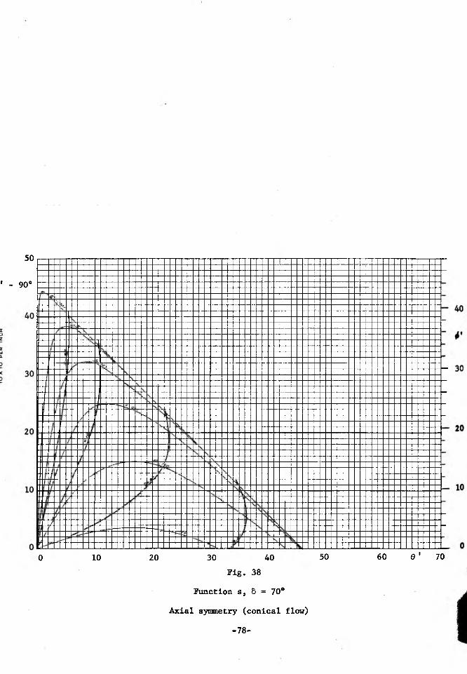
for the five values of 5: 30°, 40°, 50#, 60° and 70°. The solutions
for symmetric plane strain are shown in Figures 29 to 33, for axial
symmetry in Figures 34 to 38, and three cases of asymmetric plane
strain at 8 = 50° are shown in Figures 39 to 41 for 4* m 20°, 30° and 40°.
In axial symmetry mathematical solutions are also available with a
discontinuity in \|r at the axis of symmetry. However, these solutions
imply s ■ 0 at the axis. This is physically unlikely to occur and,
therefore, these solutions are not computed.
While no formal proof of uniqueness of solution for boundaries
(0',^') and (-0",^") is submitted, the large number of numerical cal
culations which has been carried out seems to indicate that, within the
range of application to the physical problems under consideration, the
radial flow solutions obtained by the above method are unique.
In the discussion of Boundaries it will be indicated that in gravity
flow the fields are unlikely to extend outside of the j ■ 0 lines.
Therefore, all the plots in plane strain are bounded by the lines ] » 0
and cos - sin 6 ■ 0. In axial symmetry the available solutions
cover more restricted regions in the (0,^) coordinates and do not reach
the above specificied lines. Indeed, in axial symmetry, for solutions
with velocity discontinuities at the walls to exist, the walls must be
i
sufficiently weak. For instance, it is most unlikely that axi-symmetric
converging flow can occur withih sliplines. However, flow without
velocity discontinuity is possible within rough walls. In such flow,
the walls are velocity characteristics, which means that i|r1 “ 3rt/4 and
\|/" ■ n/4. A value oft* - 90° ■ 45° cuts across the regions of solution
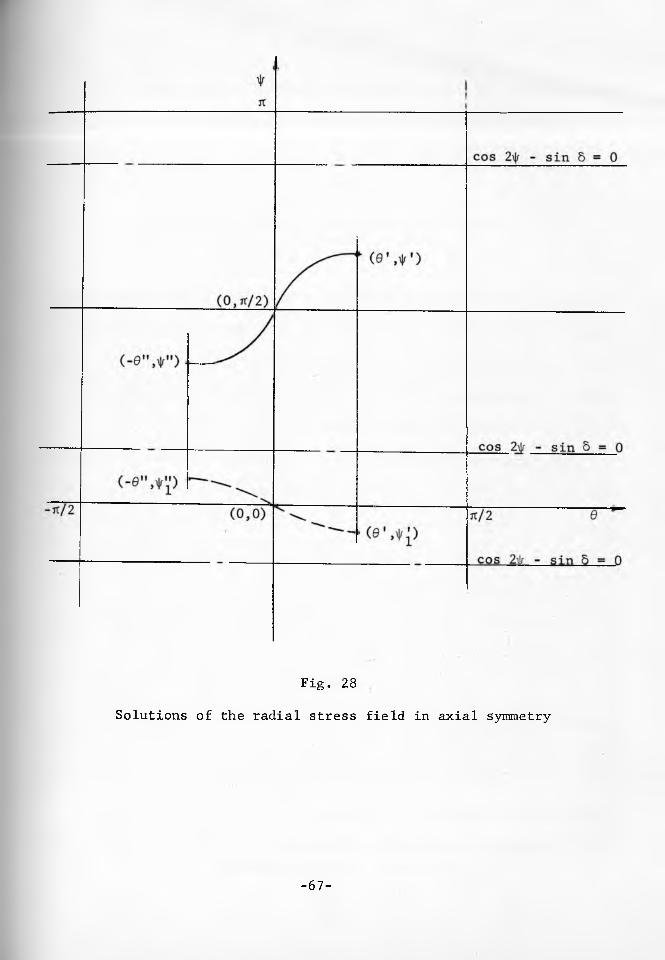
Fig. 28
Solutions of the radial stress field in axial symmetry
-67-

and indicates the largest possible value of S' within rough walls.
These values of Q r are listed in Table 2 as a function of 5.
T ab 1 e 2
5 30° 40° 50° 60° o 0
Max. S' 15° 8 „ 1° 4.4° 2.2° .5°
Especially, for the larger values of 5, an axi-symmetric channel can
open out but very little. In addition, this type of flow implies a
continuous velocity profile at the top and at the bottom of the channel
and is, in practice difficult to attain. As a result, this type of
flow, if it occurs, is usually unsteady.
Resultant vertical force. It is of practical interest to know the
resultant vertical force Q acting at a horizontal cross-section of a
channel. An expression for this force will now be derived. The hori
zontal cross-section is of width B = 2 y ', and is elevated a distance
-x0 above the wertex, Fig. 42.
The vertical pressure a is found from e q .(14) with substitutionsX
(3) and (102) for to and a , thus
a = r y s [1 + sin 5 cos 2(\|r + 0)] „X
The total vertical force is
. „ m _ 1-m rV1 m ,Q = 2rt L F a y dy, (j)
\J X
where L is the length of the channel in plane strain. To compute Q
it is necessary to express y as a function of x Q and the angles 8 and \|f.
-68-

Function s, 8 = 30°
Plane symmetry (symmetric plane flow)
-69-

0 10 20 30 40 50 60 6 ' 70
Fig. 30
Function s, 6 = 40°
Plane symmetry (symmetric plane flow)
-70-

70
i|r'- 90°
60
50
40
30
20
10
0 E20 30
Fig. 31
Function s, 6 = 50°
Plane symmetry (symmetric plane flow)
-71-
60 6' 70

10
X 10
PER
IN
CH
— 50
60
40
— 30
— 20
10
Fig. 32
Function s, 5 =• 60°
Plane symmetry (symmetric plane flow)
-72-

Function s, S = 70°
Plane symmetry (symmetric plane flow)

60
0 10 20 30 40 50 60 0 1 70
Fig. 34
Function s, S = 30°
Axial symmetry (conical flow)
-74-

Fig. 35
Function s, 5 = 40°
Axial symmetry (conical flow)
-75-
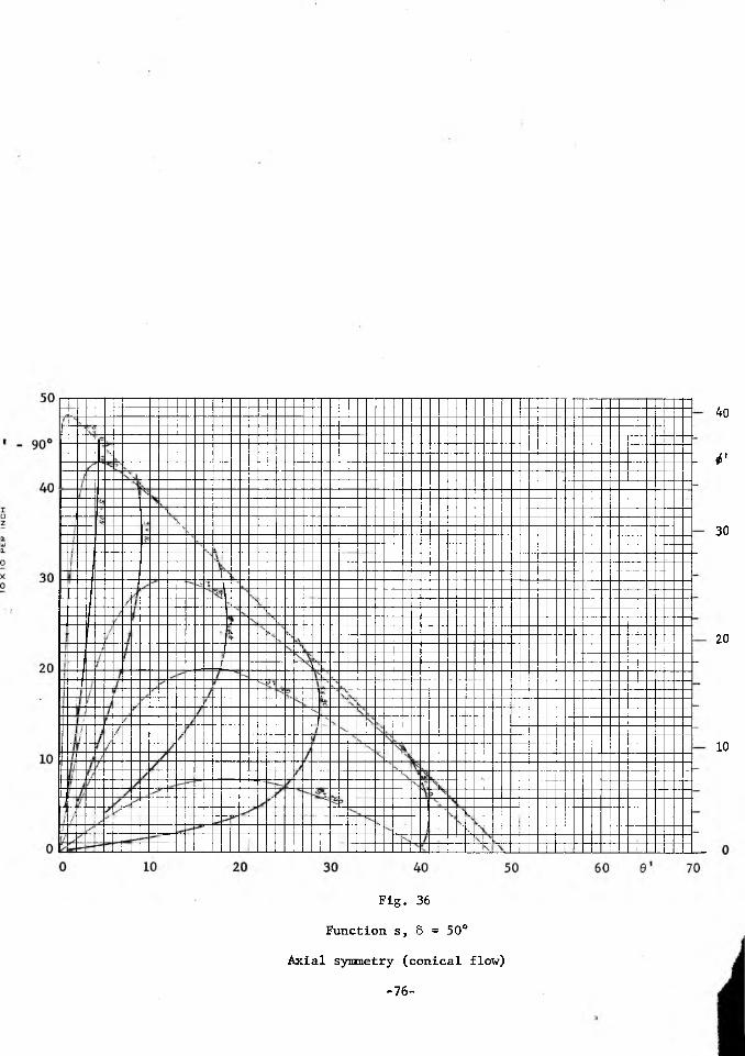
Fig. 36
Function s, 8 = 50°
Axial symmetry (conical flow)
-76-
V
30
40
20
10

Fig 37
Function s , 8 = 60*
Axial symmetry (conical flow)
-77-
50
' - 90°
0 10 20 30 40 50 60 0 1 70
Fig. 38
Function s} S = 70°
Axial symmetry (conical flow)
-78-
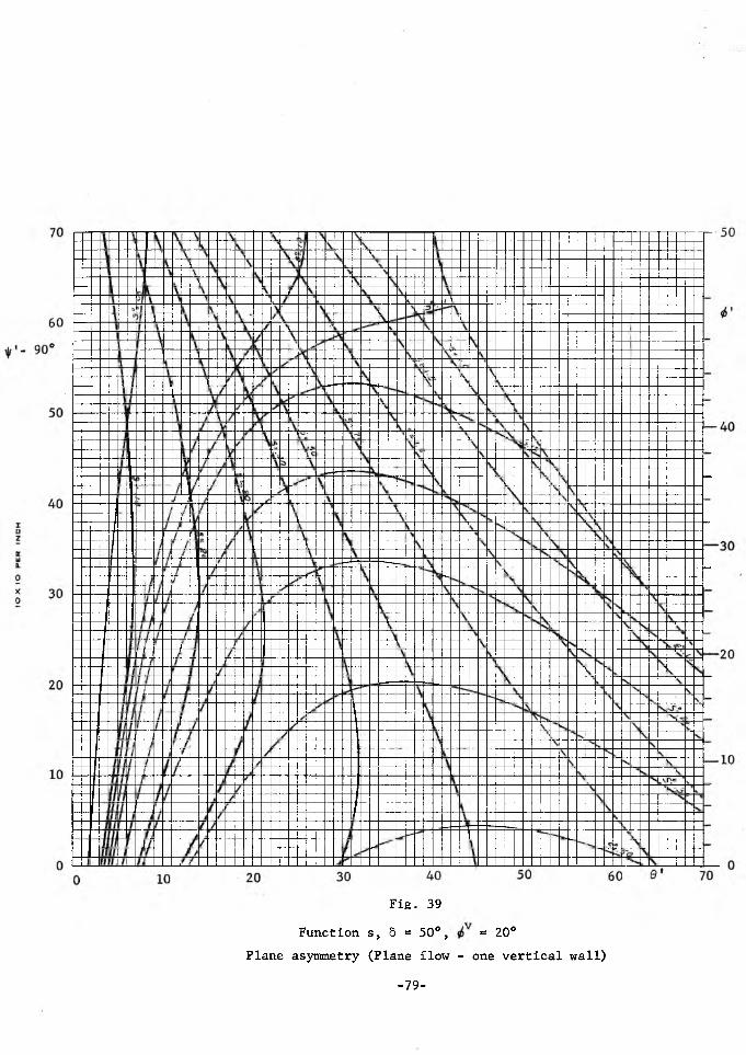
Fig. 39
Function s, 5 = 50°, = 20°
Plane asymmetry (Plane flow - one vertical wall)
-79-

t'- 90
Fig. 40
Function s, 5 = 50°, = 30°
Plane asymmetry (Plane flow - one vertical wall)
-80-

Fig. 41
Function s, 5 = 50°, = 40°
Plane asymmetry (Plane flow - one vertical wall)
-81-

} (k)
The relations between the (x,y) and (r,0) coordinates are, (Fig. 2),
x = - r cos
y = - r sin
The total derivatives are:
dx = -cos 0 dr + r sin 0 d0 ,
dy = - sin 6 dr - r cos 0 d 0 .
For x 0 constant, dx = 0 and elimination of dr between the above
two equations leads to
, r d0dy " ' ^ T e - (1)
From conditions at the wall, Fig. 42, there is
x 0 = y 1 cot 6 1.
Within the channel
, r = - X° 'cos
or, eliminating x 0 ,
y'cot 0'r =
cos
Hence expression (1) for dy becomes
dy = y' cot_ o ._d0_2
cos 0
Elimination of r in the second of equations (k) yields
y = y r cos 0' tan 0.
Substitutions for a , r, y and dy in eq.(j) transform it intox'
where
Q = q r L 1_m B2+m, (103)
, 2+m 0 1 mq = 2itm (-°-- ■■) / s — [1 + sin S cos 2(0 + i|r) ] d 0 . (104)
° cos 0
-82-
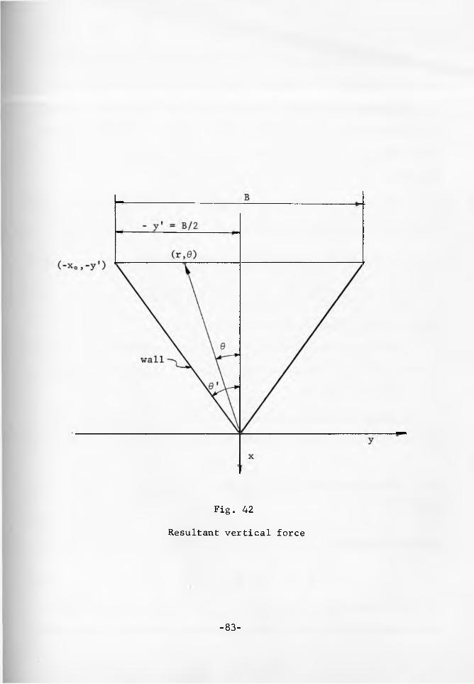
Fig. 42
Resultant vertical force
-83-
Lines of constant values of q are plotted in Figures 43 to 48 for
5 = 30°, 40° and 50° in symmetric plane strain and in axial symmetry.
Stresses at the w a l l s . The normal and shearing stresses a' and t'
which act between a flowing solid and the walls are computed from equa
tions (18) and (19): a' = Oq and t ' = - ,respectively. In these
equations, a is replaced by expression (102) with
Br =
2 sin 0 ’
in accordance with Fig. 49, leading to
___ _______,1 - sin 5 cos 2\|f'T B r B 2 sin 0' ’ U }
, sin S sin 2\lr1(106)
r B r B 2 sin 0' •
These equations apply in plane and axial symmetry.
Lines of constant values of 0 !/Y b and t '/Y B are plotted in figures
50 to 61 for plane strain and axial symmetry in (0',o') coordinates
for 6 = 30°, 40° and 50°.
Influence of compressibility. The influence of compressibility
on the solutions of radial flow can be estimated by using the expression (27)
Y = YoC^
with a eliminated by means of eq.(102) to yield
1
Y = (rf3YoSP ) 1"P , (107)
and the derivatives
1 dr _ P 1 ds r S Y = P n n R *Y c*0 1 ■ P s d 0’ T ^ r 1 - p' U ;
With these substitutions, and = \|/(0) for the radial field, the
coefficients (87) to (90) of the differential equations (85) and (86)
-84-

k'
Fig. 43 -
Vertical force q, 6 = 30°
Plane symmetry (symmetric plane flow)
-85-

Fig. 44
Vertical force q, 5 = 40°
Plane symmetry (symmetric plane flow)
-86-
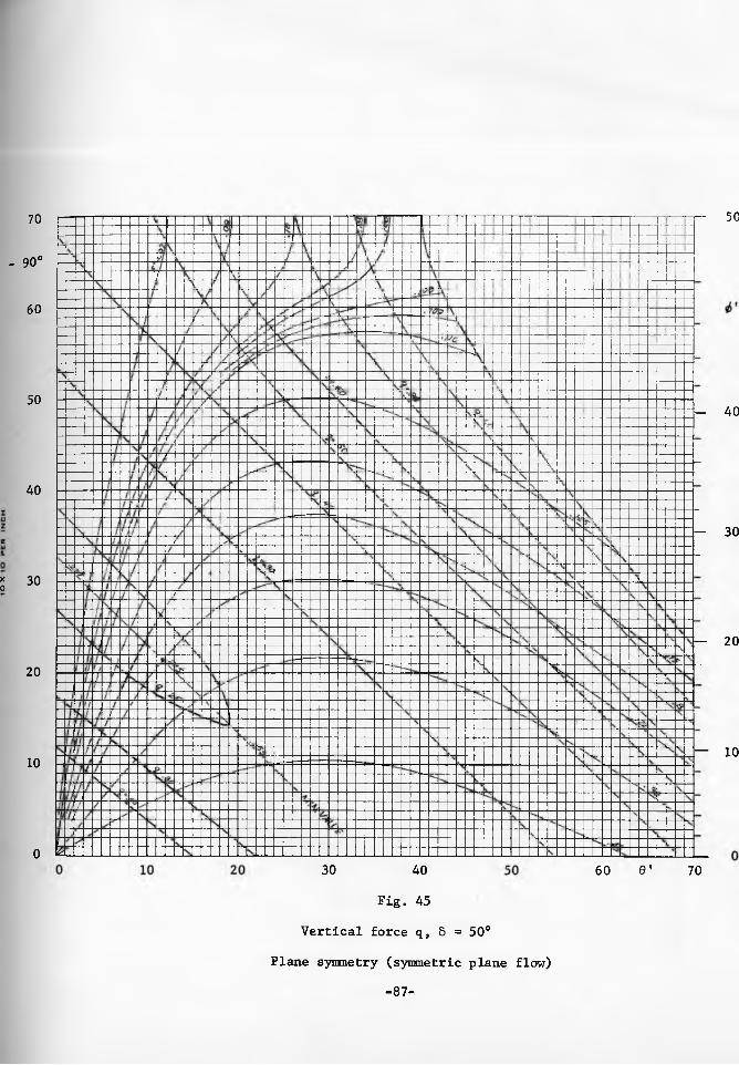
70
- 90°
60
50
40
s 30
20
10
0 E
50
- 40
- 30
— 20
— 10
30 40
Fig. 45
Vertical force q, 5 = 50°
Plane symmetry (symmetric plane flow)
-87-
60 O' 70

20 30 40 50
Fig. 46
Vertical force q, 8 = 30°
Axial symmetry (conical flow)
-88-
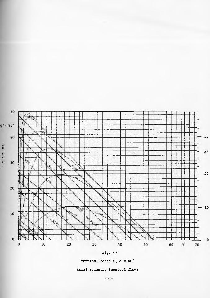
10
X1
0
PER
IN
CH
30
20
— 10
Fig. 47
Vertical force q, 5 = 40°
Axial symmetry (conical flow)
-89-

Fig. 48
Vertical force q, 5 = 50°
Axial symmetry (conical flow)
-90-
- 40
h- 30
— 20
- 10

F i g . 49
Stresses at the walls
-91-
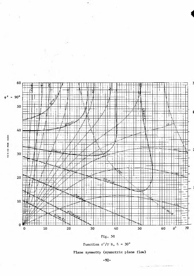
i
Fig. 50
Function cr'/V B, 5 = 30°
Plane symmetry (symmetric plane flow)
-92-

- 1
10 20 30 40 50
Fig. 51
Function j '/T B, 5 = 40°
Plane symmetry (symmetric plane flow)
-93-
60 e' 70

Function ff'/V B, 5 = 50°
Plane symmetry (symmetric plane flow)

0 10 20
Fig. 53
Function a'/T B, 6 » 30°
Axial symmetry (conical flow)
30 40 50
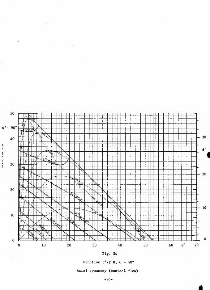
Fig. 54
Function cr'/Y B, 8 = 40°
Axial symmetry (conical flow)
-96-
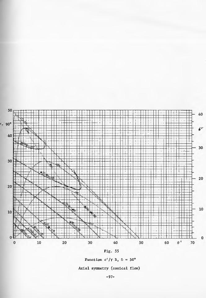
Fig. 55 Function cr'/T B, 5 = 50°
Axial symmetry (conical flow)
-97-

20 30 40 50
Fig. 56 Function t '/t B, 8 = 30°
Plane symmetry (symmetric plane flow)
-98-
30
i'
20
10
0
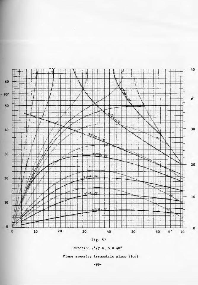
Fig. 57
Function t'/T B, 5 = 40°
Plane symmetry (symmetric plane flow)
-99-

70
- 90°
60
50
40
30
20
10
20 30 40 50
Fig. 58
Function t '/t B, 5 = 50°
Plane symmetry (symmetric plane flow)-100-
i'
30
20
10

Fig. 59 Function t'/tB, & = 30°
Axial.symmetry (conical flow)
- 101-
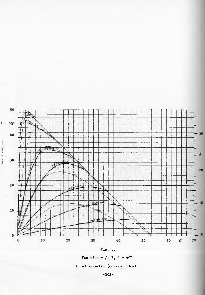
Fig. 60
Function x'/T B, S = 40°
Axial symmetry (conical flow)
- 102-
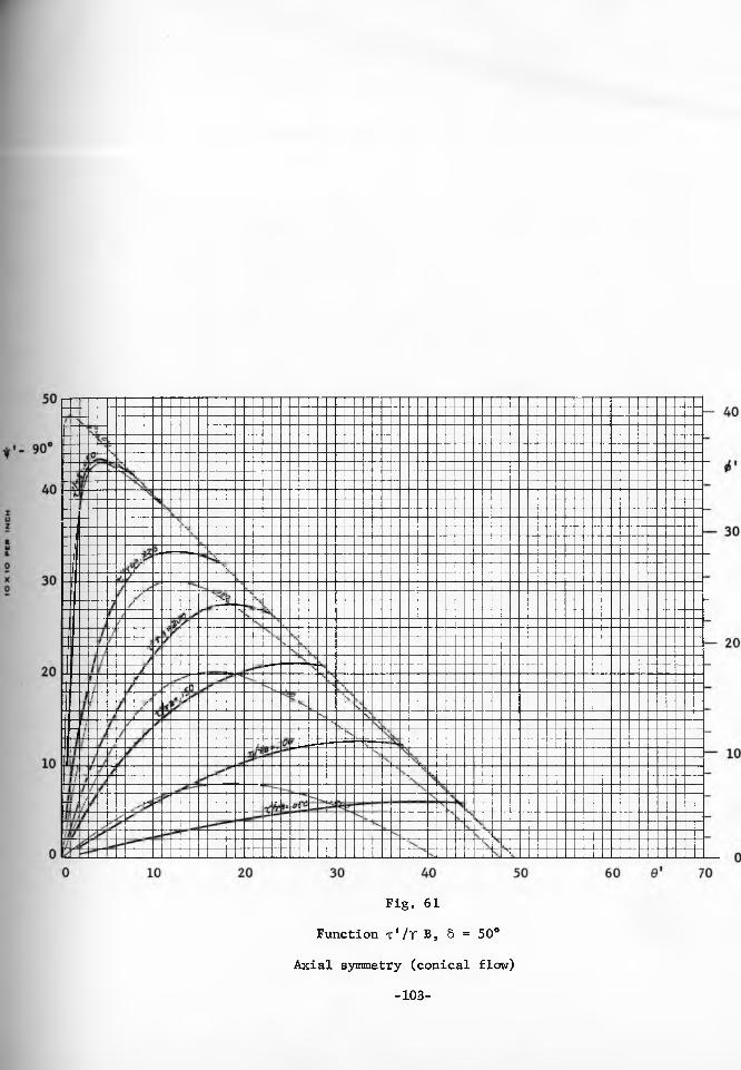
Fig. 61
Function t '/t B, 5 = 50°
Axial symmetry (conical flow)
-103-
become
f(0) = (1 - P){2(^| + D ^ ~ sin 2* + cos 5
+ m (1 + sin 5) [sin 2\Jr - cot 0(1 + cos 2\|/) ]"| , (109)* J
g(0) = - (1 - sin(0 + 2t) + ^ ^ 1 , (110)cos S cos S
h(0) = 'Y~7~b + 2(d0 + D (cos " sin 6)""n2“ +cos 5
+ m ^ (1 + sin 5) (cot 0 sin 2\|r + cos 2^ - 1) , (111)
cos 5
j(0) = - cos(0 + 2\|r) + C°S20 » (112)cos 5 cos 6
and the differential equations reduce to the form (98) and (99) as for
an incompressible solid. Equations (98) and (99) with the above coeffi
cients are now solved for the derivatives
HJ = $(0,t,s) =
* - 1 - | m s sin 8(1 + sin 8) (cot 0 sin 2i|r + cos 2\J/ - 1) + cos 0 +
- sin 8 cos(0 + 2\|f) 4- s cos^S/(l -|3)|/2s sin 8(cos 2\|r - sin B)? (m)
4§ -r(0,t,s) =
f s sin 2f , . \ ,= | i _ (3 s m ( 0 + 2i|/) +
+ m s sin 5 [cot 0 (1 + cos 2\|/) - sin 2\|r j) 0 . --- I— r1 (n)Y Y JJ co s 2tJt - s rn 8
-104-
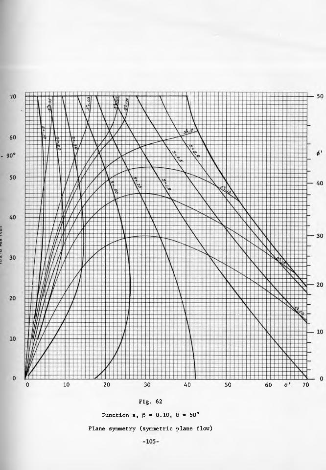
0 10 20 30 40 50 60 Q' 70
Fig. 62
Function s, P =* 0.10, 6 = 50°
Plane symmetry (symmetric plane flow)

lO
X to
PE
R
IN
CH
0 10 20 30 40 50 60 6' 70
Fig. 63
Function s, (3 = 0.10, 5 = 50°
Axial symmetry (conical flow)
-106-

The above equations are equivalent to the integral equations
\|r(0) = \|r(e°) + f6 ® [ t , t ( t ) , s ( t ) ]dt, (113)0°
s(0) = s(0°) + f [t,t(t),s(t) ]dt, (114)0°
from which the functions i|r and s are computed in the same way as for
incompressible solids.
In order to estimate the quantitative effect of compressibility,
several numerical calculations were carried out for £3 = .10, which is a
rather extreme value. Function s(0) is plotted in Figures 62 and 63 for
symmetric plane strain and for axial symmetry with 5 = 50°. A compar
ison with the corresponding values fox- an incompressible solid, Figures
31 and 36, shows that the influence of compressibility is small.
It should be noted that these equations apply at some distance
from the vertex where cr[ lb per sq ft] » 1„ For (3 = 0, these equations
reduce to the form obtained for incompressible solids.
General stress field
Proof of convergence to a radial stress field at the vertex. The
significance of the radial stress field is greatly enhanced by the fact
that all useful stress fields converge to radial stress fields at the
vertex. This statement will now be proved under the assumption that \|/, T
and their first derivatives are continuous in a sufficiently small
neighborhood of the vertex. This assures the continuity of f, g, h, and
j, equations (87) - (90).
-107-

Eq. (85) is integrated to yield
-/p0f (r,t)dt -/qo f (r, t)dt /Lf(r,u)dus(r,0) = s(r,0°)e -e /0Og(r,t)e dt. (115)
These integrals are bounded over a field satisfying the above conditions
of continuity. Therefore,
| s (r ,0) j < J s (r ,0° ) | + M2
for some constants and . Hence, if there is one angle 0° for which
j s(r,0°) | < °°,then
| s (r ,0) | < °°
for all values of 0 within that field.
Eq„ (86) is now integrated, yielding
-,-r _fr M M > dt r . . /:(r,8) - s(r0,0)e r" C -e r° 1 / J % ^ e r° t*&d»r. t - dt- <U 6 >
where r0 > r.
The value of this function will now be analyzed in the limit as
r o . It will be observed that the signs of lim h and lim j play anr o r o
important role in the analysis, and the following two cases are distin-
gulshed: _; r h(t.e)1. Lim h < 0, lim ] f 0. In this case lim e r° C =0, the
r^s-o r ^ o r^-o
first term of eq. (116) vanishes, while in the second term
rt h(u,0) ,fr i(t,e) r„ u u lim / ’— ° dt = “ . The second term is evaluated by usingrQ tr->o
L'Hospital’s rule, yielding
-108-

,r M u ^ l duj j(t;9) e r0 u dt
lim s (r,0) = lim - t ----------- = lim ' h ^ f f (117)r+o r*o J h(t,0)^ r*o
r0 ue
It will be noted that the boundary value s(ro,0) does not affect lim s(r,0),r»o
and that, in this case, no condition is imposed on the value at the
boundary.
_;r M ^ l dtx ^2. Lim h > 0, lim j f 0. Now lim e ° = °° and, for a
r->o r^o r*o
useful solution to exist, it is necessary that the boundary value
satisfy the condition
ft h(u,0)* ( p) \ J du
s(ro,0) = lim / ?— e r° U dt, (118)r»o r„
then, as in the case 1, the application of L'Hospital's rule yields
lim s(r,0) - lim - r*o r-so ’
The satisfaction of the condition (118) implies s(ro,0) ^ 0, i. e. no
traction-free boundary, within the region of 0 in which lim h > 0.r»o
If the condition (118) is not satisfied, then lim s(r,0) = <». While
a mathematical solution may exist in the neightborhood of the vertex,
the large values of s and, in turn, the relatively large values of
pressure a in the region of the outlet of the channel would consolidate
a real solid to a degree likely to cause the development of a stable dome,
-109-

and flow would fail to develop. Hence, it is expected that in physical
channels condition (118) is satisfied.
The physically acceptable solutions are further restricted by the
condition that the solid does not transfer tensions, hence, s(r,0) > 0 .i (r O')This implies lim - — 2— r > 0 and requires: in case 1, lim h < 0,
r*o ’ r-*-o
lim j > 0; in case 2, lim h > 0, lim j < 0. To conform with this condi- r*o r»o r*o
tion, the change of sign of lim h and lim j must occur along the samer-yo r^o
ray 0. It is easy to show that the latter is also necessary for a
bounded solution to exist along that ray,
t^ M £ t0ldte
r*o r*o27 t -because for lim h = 0 , lim e is finite and non-zero, while
,fc h(u,0) , r i(t 0) ^ro””V ”lim / 3— e ° dt = 00 and, hence, lim s(r,0) = °°, unless lim j = 0
r>o r° ' r-»o r-»o
The significance of the direction established by lim j = 0 will ber*o
further discussed in the next section on Boundaries.
It has thus been shown that the useful solutions of the equations (85)
and (86) approach the form (117) in the neighborhood of the vertex.
It will now be shown that lim s(r,0) of eq.(117), is the same as s(0),r*o
eq.(97), obtained for the radial stress field.
In view of the relation (117), eq.(86) may be written
where
s h(r,0) + j (r,0) = e19
lim e = 0 . r- o
-110-
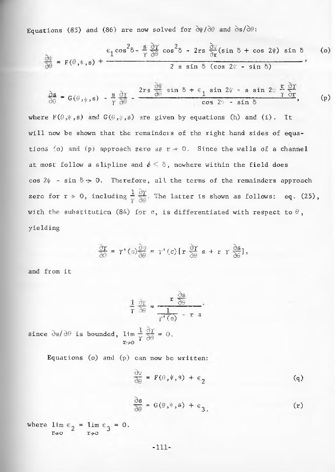
Equations (85) and (86) are now solved for d\j//d0 and ds/d0:
e^cos^S- cos^S ~ 2rs ^(sin & + cos 2\|r) sin 8 (o)
F( ,!/,&) 2 s sin 5 (cos 2if - sin 8)
x 2rs 'nt: sin 8 + e, sin 2if - s sin 2f — r—ds _ _/r. N s dr 66______________ 1_________________ r or , sd0 G(e,^,s) - r - cog 2i)f _ sin 5 > (p)
where F (0 ,i|/, s) and G(0,i|/,s) are given by equations (h) and (i) . It
will now be shown that the remainders of the right hand sides of equa
tions (o) and fpj approach zero as r -*• 0. Since the walls of a channel
at most follow a slipline and < 8 , nowhere within the field does
cos 2\|; - sin 8 -> 0. Therefore, all the terms of the remainders approach1 drzero for r -» 0, including — . The latter is shown as follows: eq. (25),
with the substitution (84) for a, is differentiated with respect to 0 ,
yielding
dr , / v M . , ST dr , ds-.30 - r - r ' t o l r ^ a + r r 5 l ,
and from it
ds1. d r _______r d0r de ~ i
r ' ( o ) ~ r 3
1 Stsince ds/d0 is bounded, lim — r— = 0 ,’ r d 0r-»o
Equations (o) and (p) can now be written
df = F(0,^,s) + e2 (q)
ds = G(0,t,s) + e3 (r)
where lim = lim 6 = 0 . r^o r -o
-111-
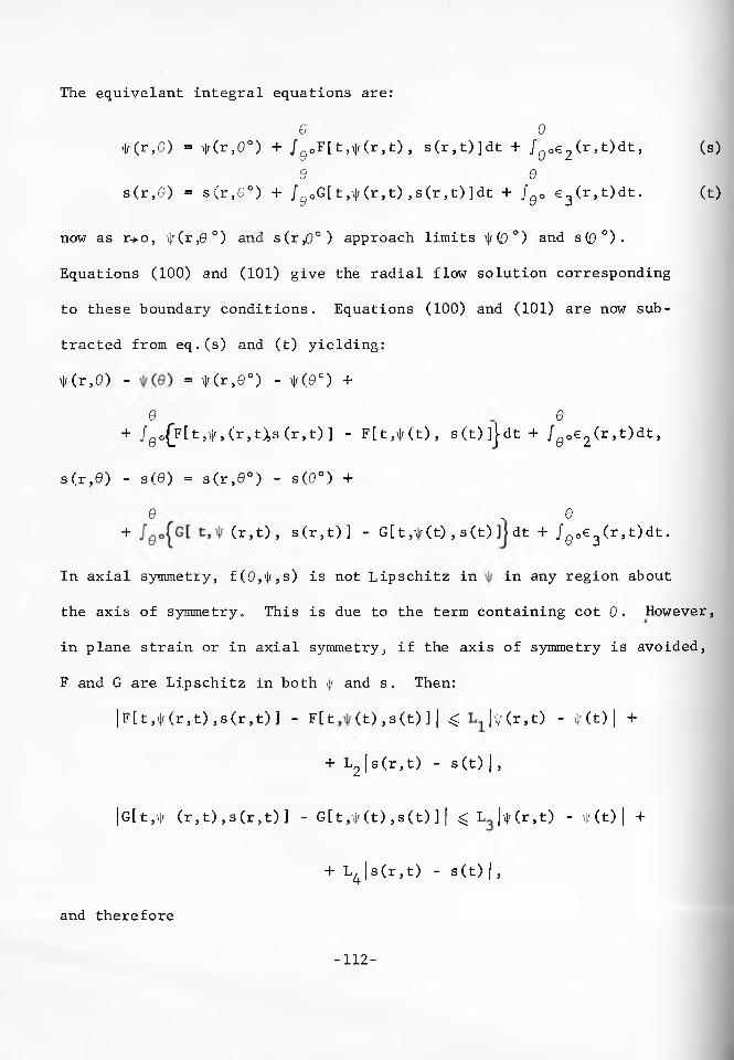
The equivelant integral equations are:
0 0 t(r,e) = t(r,0°) + /0OF[t,\|r(r,t) , s (r, t) ] dt + JQOe 2 (r, t) dt, (s)
e es(r,0) = s(r,0°) + /g0G[ t ,\|r (r, t) , s (r, t) ] dt + JQO e3(r,t)dt. (t)
now as r+o, \|/(r,0 °) and s(r,0°) approach limits \|r(0 °) and s(0 °).
Equations (100) and (101) give the radial flow solution corresponding
to these boundary conditions. Equations (100) and (101) are now sub
tracted from eq.(s) and (t) yielding:
\|r(r,0) - = ^ ( r , 0 ° ) - \K0°) +
0 6 + /eo F[t,\|r,(r,t),s (r,t) ] - F[t,\|/(t), s(t)]|dt + IQo&2 (r, t) dt,
s(r,0) - s(0) = s(r,0°) - s(0°) +
0 . 0 + (r,t), s (r, t) ] - G[t,t(t) , s(t) dt + /@ oe 3 (r,t)dt.
In axial symmetry, f(0,\|r,s) is not Lipschitz in in any region about
the axis of symmetry. This is due to the term containing cot 0. However,
in plane strain or in axial symmetry, if the axis of symmetry is avoided,
F and G are Lipschitz in both \|r and s. Then:
|f [ t ,\[r (r, t) , s (r, t) ] - F[ t (t) , s (t) ] j ^ Jlr (r, t) - \|r(t) | +
+ L2 |s(r,t) - s(t)|,
|G[t,\|r (r,t) ,s(r,t) ] - G[ t ,t (t) ,s (t) ] | ^ L |t(r,t) - \|f(t)| +
+ I7J s (r, t) - s (t) | ,
and therefore
-112-

|\|r (r,0) - Hr (0)1 ^ |^(r,0°) - ^ (0°) | +
0 0 + ■0°[L1|\lf(r,t) - \Jr (t) | + L2 js(r,t) - s(t)|]|dt| + J Qt> | e2(r,t) | |dt | ,
|s(r,0) - s(0)| |s(r,0°) - s(0°) | +0 0
+ /0O[L3 |t(r,t) - i(r (t) | + L4 |s(r,t) - s(t) | ] |dt| + / 0 o |e3 (r, t) | jdt j „
These inequalities are now added, yielding:
0°Kr,0) <C L /0Oar(r,t) Jdt I + |3(r,0,0u), (u)
where:
a(r,0) = |^(r,0) - \|r(0) | + |s(r,0) - s(0)|,
P(r,0,0°) = | i|r(r,0°) - 1(0°) | + |s(r,0°)- s(0°)| +0
+ /go[|e2(r,t)I + |e3(r,t)j ] |dt j
and L = max^ Lp L^, J.
The method of successive approximations, used on (u) yields:
a (r,0) ^ P(r,0 ,0°) e L l9 + 8 'L (v)
But lim (3(r,0,0°) = 0 and, therefore, lim CC(r,0) = 0, or r->o r- o
lim i|r (r,0) = ilr (0) , (w)r-»o
lim s(r,0) = s(0). (x)r-»o
The significance is this:
Given a converging stress field satisfying the conditions stated
in this proof, and a ray 0 = 0° along which \(r(r,0o) and s(r,0°) approach
limits \K0°) and s(0°) as r-»o, there is a radial stress field given by
-113-

i|/(8) and s(0) from eqs.(lOO) and (101), with boundary conditions i|/(0°) and s(0
such that throughout the field ty(r,0) ->i|r(0) and s(r,0)-»s(0) as r_^o. Althou
the proof, as given, does not hold if 0 and 0° are separated by 0 = 0 in
axial symmetry, the axi-symmetric field is completely determined if it is
known on only one side of 0 = 0. Hence the axis, 0 = 0 , need not be
crossed.
Boundaries. A general problem satisfying equations (85) and (86)
is defined by the specification of adequate boundary conditions. Such
conditions are ilr0 = \|/o(0) and s0 = so(0)} at the top boundary, and
i|r' = \|r1 (0) , \|r" = t"(6), at the walls, Fig. 64. The stress field is
then defined down to the stress characteristics passing through the end
points of the walls. Hence, the stresses at these two points are inde
pendent of the bottom boundary conditions, and, as has been shown in the
previous section, approach the magnitude of the appropriate radial stress
field. This is important, because these two stresses are used in the
derivation of the flow criteria which are, therefore, independent of
the top boundary. This justifies the development of the design criteria
on the basis of the radial stress fields and eliminates the need for a
large number of particular solutions of general fields. Several general
fields are discussed in a separate publication [15].
In gravity flow, the slopes of the walls in the neighborhood of the
vertex seem to satisfy the condition lim j > 0. There is a physicalr->o
meaning to this bound, namely the horizontal component cs of the stress
vector acting on the solid from a wall, Fig. 65, is given by
-114-
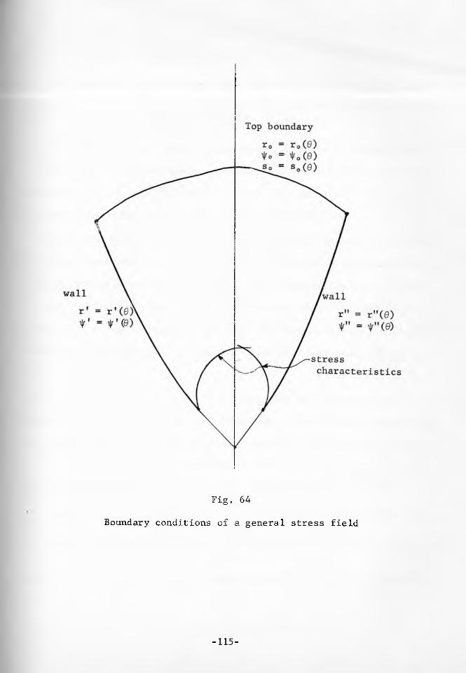
Fig. 64
Boundary conditions of a general stress field
-115-

a, = a cos 0 + t sin Q . h e re
With sibstitutions (18) and (19), the inequality cr > 0 yields
1 - sin 5 cos 2jr' - sin 5 sin 2V
_ * JL “ o l l l U U U S i -t r\\tan 0' < ----g 0"; "7, (119)
and is identical with the condition lim j > 0. The latter then implies
a positive direction of the horizontal component of the stress vector
at the wall. In a channel with a straight wall, Fig. 66, it is apparent
that, if the above condition is not satisfied, the top boundary cannot be
traction-free, but requires stresses which have a resultant force con
taining a positive horizontal component. This follows from the considera
tion of the equilibrium of the horizontal forces acting on the flowing
mass between the wall and a vertical plane through the vertex. Therc
pressure across the vertical wall cannot be balanced by H = Jo cos 6 'dr
if 0, hence the requirement for the positive horizontal component
at the top boundary.
While such top boundary conditions are possible, they are unlikely
to occur in gravity flow, and cannot occur with a traction-free boundary.
Observations of flow in physical channels confirm this conclusion: they
indicate that inequality (119) is satisfied.
The above argument tallies with the results of the analysis of the
previous section which indicated that for case 1, lim h < 0, lim j > 0,r>o r*-o
a bounded solution lim s(r,0) = lim - (j/h) is obtained for all topr»o r^o
boundary values s(ro,0); but for Case 2, lim h > 0, lim j < 0, a boundedr -o r-f-o
-116-

Fig. 65
Stress vector at a wall
Fig. 66
Equilibrium of a flowing mass
-117-

solution requires the satisfaction of the condition (118) for the top
boundary stress.
There thus seems to be sufficient reason to limit the considera
tion of the radial stress fields (which occur in the neighborhood of
r->o) to regions in which j > 0 .
The substitution of expression (44) with 9' =0' in inequality
(119) yields
0' < | - </>' . (120)
For a rough wall, similarly,
9' < | - )6 .
These bounds for 9' apply only in plane strain. In axial symmetry,
the acceptable solutions of the radial stress fields occur within
regions of (9,10 which are more restricted than the bound j = 0 , cos 2i\r - sin 5 = 0.
The shape of the walls, r' = r'(0) and r" = r"(9), away from the
vertex, is a function of the shape of the top boundary, r0 = rQ(9),
and the functions = ^ 0(9), s0 = s0(9) along the top boundary. In
gravity flow, the top boundary usually varies within wide limits
and,therefore, the shape of the walls should vary accordingly. How
ever, this is possible only when a solid flows within itself and forms
its own rough walls. Even then, the free adjustment of the shape of
the walls is inhibited by the fact that a solid develops cohesion at
different rates in the plastic and in the rigid regions . In the
rigid regions, the time effect comes into play and, after a while
the rigid regions may, in effect, behave as if they were made of a
different solid and a plane which is weak with respect to the
-118-

rigid solid may develop along the walls.
When the channel is built of weak walls, the solid will flow along
the walls, provided the walls are sufficiently steep and do not contain
sharp corners. Typical shapes of channels are discussed in Chapter VI.„
Radial velocity fieltj.
As was shown in the previous section, radial stress fields are
approached in all channels in the vicinity of the vertex. A radial
velocity field is compatible with a radial stress field. It should be
emphasized that there is no unique velocity field which corresponds to
a given stress field and that there are other velocity solutions
compatible with a radial stress field. Indeed, radial velocity fields,
which include the lines \|r = Jt/4 and \|r = 3Jt/4, are physically unacceptable
because these fields require velocity to be zero along these lines and,
in some cases, also require a velocity discontinuity along these lines,
which is impossible since they are not sliplines. However, for wall
conditions \Jr' < 3n/4 and \|r" > rt/4, the radial velocity fields closely
represent the fields observed in physical channels. Since velocity
fields are subject to superposition, the radial field provides one
readily obtainable solution which can be combined with other fields to
satisfy the required boundary conditions.
It will again be convenient to use polar/spherical coordinates. The
equation of continuity in steady state flow is
!^[yurr(r sin 0)m] + -^[rUgCr sin 0)™] = 0 , (121)
-11.9-
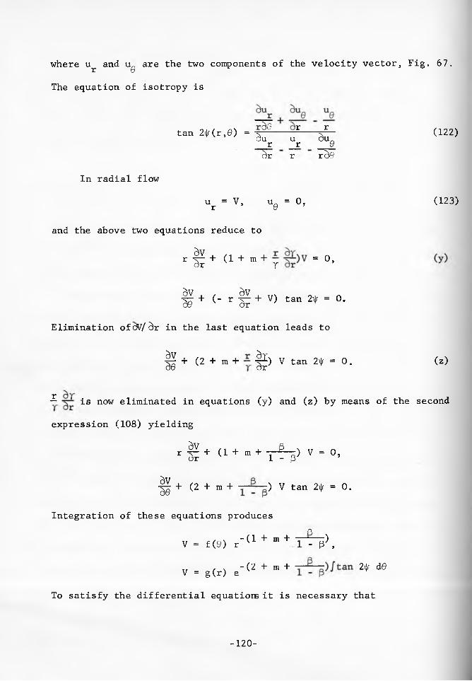
where u and u are the two components of the velocity vector, Fig. 67. r U
The equation of isotropy is
In radial flow
“ 2*<'-e> ■ a f ur a l <122>_r _r __0dr r rdO
ur = V, uQ = 0, (123)
and the above two equations reduce to
r I? + (1 + m+ y = °>
|| + (- r || + V) tan 2f = 0.
Elimination ofcSV/dr in the last equation leads to
|^ + (2 + m + |^) V tan 2\|/ = 0. (z)
X*— is now eliminated in equations (y) and (z) by means of the second
expression (108) yielding
r i + <1 + " + r ^ p > v - ° -
|| + (2 + m + - ) V tan 2^ = 0.
Integration of these equations producesO
V » £(e) r ' < 1 + m+ r r p ) ,
V - g(r) e"<2 + m + 2t d8
To satisfy the differential equatiorB it is necessary that
-120-

Fig. 67
Velocity components in polar-spherical coordinates
-121-

f(0) - e'<2 + " + I?p)/tan 2* dlS and
t \ - (1 + m + t%t) g(r) = r 1-p ,
which enforce
^ = ^(6) ,as was assumed by the eq.(91) in the radial stress field.
The expression for the velocity is
o 1 + m + - (2 + m + T^r)/fl0 tan 2^ d0. (124)V = V° (— ) 1_P e 1_P 6 *r
It will be noticed that along the rays xjr = 3it/4 and i|f = it/4, tan = °°?
and V = 0. The derivative 3V/S0 along one of these rays, e. g.
\|f = it/4, will now be determined. Eliminate V in eq. (z) to obtain
|| - F(r) tan 2* e‘(2 + ” + 2* d0.
It is necessary to find the limit of cOV/bO as 0 approaches the value at
which \|/(0) = it/4. The function is rewritten as follows
6 Q
|| - F(r) tan 2* e'(2 + m + T ^ e ° tan 2* d6 e‘(2 + n + T ^ e ^ " 1 2t d®
where 0^ is a constant, while 0 - 0^ is arbitrarily small. The first exponential is constant and the function can further be transformed into
Q AQ I ^Tji / \ j_ 0. -(2 + m + To ) [ j?o'; \ ] /. tan 2i|/ d (2\|r)^ = c F(r) tan 2i|r e 1-P d(2\j/)J v Y ,i
where d0/d(2>Jr) is evaluated in the interval \|r - i|r. Then, through
integration,
n + — + .ft- ir— ^' iSv s . ,cos 2i|r 2 2(1-B) dilr "Se C F(r) t m ^ (cos 2*'>
-122-

r -j + JB 4- — ft i (— 'f _ i= c!F(r)sin 2\(/(cos 2^) 2 2(l-f3) dvjr .
In the limit
dV f m P , d0 i ,m °°» f°r t1 + 2 + I 7 Fiy]# ' 1 < 0 ’
Lim§|->0, for [1 + f + 2 ^ 1 ) ] ^ “ 1 > °*
For incompressible solids, (3 = 0, and the limits are tabulated
below:
Table 3
Limit Planestrain
Axialsymmetry
00
i—1A di > 3 de 2
=de 0
— - .^ < ide
di . 3de 2
It should be noted that the above expressions for P > 0 apply only
at some distance from the vertex of the channel where a[ lb. per sq.ft.] » 1.Typical radial flow profiles are shown in Fig. 68 for the two Sv/Se
limits. In both cases velocity is zero along the two rays i|r = 3n/4 and
\|r = Jt/4. These two rays coincide with velocity characteristics and, of
course, are streamlines. The profiles shown in the figure are physically
acceptable only within the internal region, that is for channels with
weak walls whose wall yield loci intersect the Mohr stress circle within
the arc T'MT".
-123-
Lines of constant velocity in the internal regions for f3 = 0 are
shown in Figures 69 and 70 for plane strain and axial symmetry for
5 = 50°. These lines show ratios V/V° along an arc r = r° and, therefore,
in accordance with eq. (124) present the function
0| o = e~(2 + m H tan de. (125)
Vertical channels
Vertical channels are a limiting condition of converging channels.
However, the relations derived for flow in converging channels are not
suitable for application to vertical channels, hence the latter will
now be considered separately.
The radial stress and velocity fields of the converging channels
go over to fields independent of the vertical coordinate x in vertical
channels. The solutions to such fields in vertical channels are obtain
ed in closed form. There is one major difference between converging
and vertical channels. In the former there is no doubt as to the
value of the circumferential pressure: that pressure is major. In
the latter, assuming complete independence of the vertical coordinate,
there is no basis for the selection of either the major or the minor
value for the circumferential pressure. The physical consequence of
this uncertainty appears in the erratic and unsteady flow pattern which
is observed in tall vertical channels.
Some conclusions can be drawn, however, on the basis of compress
ibility if even a slight gradient of pressure exists in the vertical
-124-
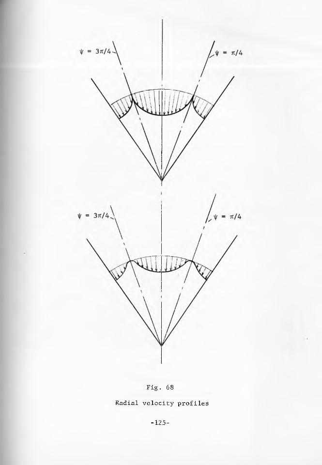
Fig. 68
Radial velocity profiles
-125-
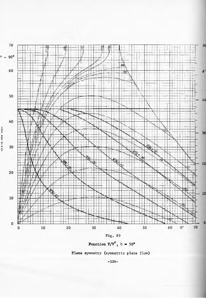
- 40
50
- 30
20
— 10
Fig. 69 Sanction V/V°, 5 = 50°
Plane symmetry (symmetric plane flow) -126-

Fig. 70
Function V/V°, 6 = 50°
Axial symmetry (conical flow)

direction. If pressure increases downward then the solid consolidates
as it flows and flow has to be divergent (k = -1) to keep each horizontal
cross-section filled out. This condition is expected to exist in the
upper part of a channel from a stress-free top surface down. In fact,
this condition seems to prevail in most channels.
It was shown in the analysis of the radial stress fields in axial
symmetry that fields with a velocity discontinuity at the walls can be
generated only within walls of a sufficient degree of weakness. This
limitation carries over to the vertical axi-symmetric channel with the
assumption of convergence (k = +1). Hence, it would seem that diver
gence more likely represents the actual stress conditions in a vertical
channel of moderate height, while the erratic flow, when it is observed,
may be explained by shifts of the circumferential pressure between
minor and maj or.
Stress field.
The purpose of this analysis is twofold: first, to derive an
expression for the mean pressure a, second, to find the ratio y"/ye,
where y" is the half width of the channel, and y^ the distance from the
axis of symmetry to the line of co = Jt/4. Along this line, as will be
shown in the analysis of the velocity field, rapid non-steady velocity
changes may occur and are, indeed, observed in full size channels. In
models with transparent walls this ratio can be observed, measured, and
compared with the computed values.
Plane-Cartesian/cylindrical-polar coordinates will be used. Pressure
-128-
ris found from eq.(48) which in this case reduces to
dT T+ m - s - rdy y
and, with the constant of integration evaluated at the axis y = 0,t = 0, integrates toxy
r = X-3~. xy 1+m
T is now eliminated by means of eq. (16), yielding
° (1+m) sin 5 sin 2(jd’ (126)
The ratio y"/y will now be determined. Plane strain flow isj j e --------------------------------------
considered first. Eq.(49) now applies in the fonn dcr /dy = 0, hence cr
is constant. The elimination of o between eq.(126), with m = 0, and
eq. (15) yields
\ sin 5 sin 2cb--y r 1 - sin 6 cos 2cd k u
For cjd = tc/4, this becomes
while for od” = it/4 - <4/2, it is
ii _ —H sin 5 cos ^ y l r - s i n S s i n j J ’
Hence, in plane strain, the ratio is
y" ______cos <j>ye 1 - sin 6 sin <{>' (128)
In axially symmetric flow, m = 1, and the equation of equilibrium
(49) is of the form
-129-

The substitution of expression (126) for o (with m = 1) in equations (15)
and (22) yields
1 - sin S cos 2co a — y v — —-—— —-— —y 2 sin S sin 2co ’
a = r . 1 + k sin 5y 2 sin 5 sin 2co
These expressions and the appropriate derivative are now substituted
in the equation of equilibrium yielding, after transformations,
dy _ (cos 2co - sin S) d(2co)________y (1 - k sin 5 - 2 sin 5 cos 2co) sin 2co’
which integrates into
/■., o\A,-, . ,B ,1 - k sin 5 „ ,C r>\y = c(l + cos 2co) (1 - cos 2co) i.— y~Tn~5— “ cos cu) > (129)
where the exponents A? B , C are as presented below in Table 4.
Table 4
Converging Diverging
A 1 - sin 5 2(3 sin 5 - 1 ) - 1/2
B 1/2 1 + sin 6 2(3 sin 5 + 1 )
C 2 sin 5 - 1 2 sin 5 + 13 sin 5 - 1 3 sin 5 + 1
Within the field, including the boundary oj = co", the observed fields
are of the type dcu/dy 0. Since, at the axis of symmetry for y = 0,

there is 0) = it/2, this implies1 - k sin 8 - 2 sin 8 cos 2cd 0 ,
or
cos 2cd.<; 1 - k sin 8N 2 sin 8
For diverging flow this condition is always satisfied, but for converging
flow
1 , 1 - sin 8 „— Arc cos — -- :— r- 03 it2 2 sin 8 N1 , 1 - sin 8— Arc cos — z--:--r— ,2 2 sin o
The bounds for 0) are
Table 5
8 30°
oO-4 50° ON Oo OO
0)" 30.00° 36.94° 40.61° 42.75° 44.09°
0)' 150.00° 143.06° 139.39° 137.25° 135.51°
It will be observed that these bounds match the values of 1 for 0- -0
plotted for the radial fields in converging channels, Figures 34 to 38.
At the wall, y = y", for a solid flowing on a rough wall, 2a>" = rt/2 - fa.
From this relation it is possible to determine the maximum values of fa
which will allow the formation of a vertical, converging field within
rough walls
fa Jt/2 - 20)"
This is given in Table 6
Table 6
8 30° .p o o 50° 60° OOr.
fa 30.00° 16.12° O00oo 4.50° 1.82°
-131-

These values of jf> are small for 6 > 40°, hence it would appear that this
field is unlikely to develop in most solids.
The ratio y"/y& is now computed for axially symmetric flow, as
follows: for co = Jt/4
C,1 - k sin 5, ye ' C<" 2 sin 8 > >
while for co" = Jt/4 - 6/2
ii /-I i i /\^ 1 . /nB /l - k s m 5 . / \ Cy = c(i + sin 6) (1 - s m 6) (— ---:---— - s m 6) ,I s m o
and the ratio becomes
V . /\A ,, . /nB 2 sin 5 s m 6 nC■*— = (1 + s m (6) (1 - s m <6) (1 - — ----:----- :----- ) . (130)y 1 - k s m 5 e
Velocity field
The velocity field is also computed with the assumption of independence
of the vertical coordinate. The equations of continuity and isotropy
(57) and (61) reduce tomT v y = c ,
and
du + dv tan 2<d = 0 .Since the constant of integration c evaluates at zero for y = y", at the
wall, v = 0 throughout the field. From the second equation it now
follows that u = V is constant, except possibly for co = Jt/4 and co = 3rt/4,
where the velocity field allows velocity discontinuities in V, However,
these lines are not sliplines and, therefore, steady state velocity
discontinuities do not occur along these lines. Unsteady slips are observed-
-132-

This flow pattern is shown on the photograph, Fig. 71. Since
unsteady effects cannot be. reproduced on a still photograph the steady
velocity discontinuities at the walls, where oo" = 3it/4 + 6/2 and
cd" = jt/4 - S/2, and the unsteady slips along the lines co = rt/4 and
co = 3 it/4 appear identical. The measured ratio y"/y = 1.6. While the
flow pattern of this model was almost perfectly of the plane strain
type, the front and back glass walls obviously prevent a plane strain
stress field from developing. The actual stress field deviates somewhat
from plane strain toward the axi-symmetric.
Ratio y"/ye is now computed for the plane strain stress field
from eq.(128), and for the axially symmetric, diverging stress field
from eq.(130). Tests of flowability of the solid indicate that
6 = 55°, i> = 50° .For plane strain
1.73ye
For axial symmetry
^ = 1.766"'5x ,234‘263x .310-’762 = 1.25"e
The observed value of 1.6 falls between these two bounds.
-133-
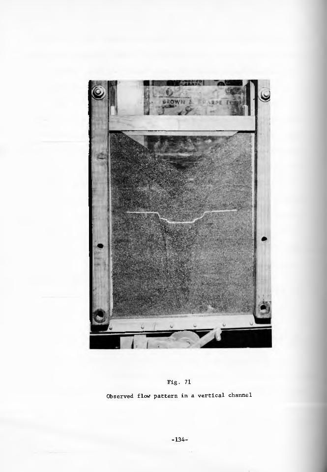
Fig. 71Observed flow pattern in a vertical channel
-134-

PART III
INCIPIENT FAILURE
General equations
The derivation of the differential equations for incipient failure
follows the pattern described for steady state flow with the following
differences: First, during steady flow the stresses are governed by
the effective yield pyramid, and are located at the edge of the base
of the pyramid. The latter implies that normality provides only a
cone within which the direction of the strain rate vector has to lie.
During incipient failure the stresses are govered by the yield pyramid,
and are located either on a face or on a side edge of the pyramid,
away from its base. Here, normality imposes either a unique direction
of the strain rate vector or a plane sector within which the vector has
to lie.
Second, in steady state flow, the solid is flowing and a velocity
field is computed. In incipient failure, velocities are zero, and an
initial acceleration field is calculated.
In earlier work [e.g. 8, 19, 20, 21] attempts have been made to
compute the velocity fields which follow incipient failure. In these
computations it has been assumed that the yield surface remains constant
as failure progresses, and that the stress field also remains essentially
constant. With the concurrent assumption of normality this enforced
continuous expansion of the solid. Since continuous expansion could
never be verified experimentally, a serious doubt was cast on the
validity of the principle of normality. This doubt appears unjustified,
-135-

the error seems to lie not. in normality but in the assumption of a
constant yield surface. The size of the yield surface certainly is a
function of density, and changes as the solid expands. In fact, as will
be shown presently, these computations produced not velocity fields
but initial acceleration fields.
The process of failure is complicated: failure seldom takes place
simultaneously throughout a stress field, usually failure occurs along
some active sliplines while regions of material bounded by those slip
lines remain rigid (or elastic). The mass becomes non-homogeneous and
unisotropic, the yield function varies across the mass with discontinui
ties along the active sliplines. The moment the first active slipline
has developed, the incipient stress field does not apply any more and
neither does the initial acceleration field. The value of the accelera
tion field associated with a stress field lies in showing that failure
can start under the prescribed boundary condition. No attempt will be
made in this work to determine how failure proceeds and how steady
state flow is ultimately approached.
The adopted yield function allows the stress equations to be solved
independently of acceleration. The solution produces the function
o>(x,y) throughout the field and the acceleration field can then be
computed. It is shown that, at zero velocity, the direction of the
strain rate vector coincides with the direction of the time derivative
of that vector, so that normality and isotropy provide the necessary
relations for the solution of the acceleration field.
-136-

Stress field
The equations are derived in plane-Cartesian/cylindrical- polar
coordinates. The two equations of equilibrium (48) and (49), together
with the equations (29) - (31), which contain the condition of
plasticity, provide a solution for the three variables (cr , a ) in v x y xyplane strain. In axial symmetry, the fourth variable Oq, is taken care
of by the additional equation (37). In these considerations, the yield
locus given by <b and f^, is assumed constant throughout the plastic
field. The equations of equilibrium are expressed in terms of cr and
CD as follows
(1 + sin <£> cos 2co) + sin <t> sin 2o) - 2a sin <b sin 2o> +
+ 2a sin <{> cos 2cd = T - m ~ sin sin 2cd, (131)
sin sin 2co + (1 - sin <b cos 2oo)| + 2a sin 6 cos 2ca +
+ 2cr sin i sin 2co = m — sin i> (k + cos 2co) . (132)dy y '
Now the following abbrevation is introduced
COt OS = — -— In •=- , (133) U0where a0 is an arbitrary constant. The differential equations then
reduce to the form
c)(S + cn) , d(S + ffl) . , , « vXT + v sn * tan(“ + 7 - f) = A > (*>Sx ay *-dUVUJ T 4 " 2;
d(S - CD) , d(S - cn) , it , viSi + 3y tan.(ai - 4 + 2> ' B~ (b)
where
-137-

In the first characteristic direction,
= tan (oj + - |) , (136)
the left hand side of eq.(a) is a total derivative
d(S + co) _ A dx
Similarly, in the second characteristic direction,
li ■ t m - 1 + 1
the left hand side of eq. (b) is a total derivative,
(137)
dx tan (co - - + -), (138)
d('S ~ ^ = B. (139)dx
The two stress characteristics intersect at an angle rt/2 - (6, and form angles "t (jt/4 - {5/2) with the direction of the major pressure.
In incipient failure the stress characteristics coincide with the sliplines.
Initital acceleration field
The equations of the acceleration field are derived on the basis of
isotropy, eq.(61), and the conditions imposed by normality on the
direction of the strain rate vector. The three principal strain rates
are ordered e. > 0, e < 0 , m k e > 0 .J. Z '-*»Following Shield's reasoning [10], normality requires

e » X,(l - sin fa) , = -(A. + M-) (1 + sin fa) , m ea = p.( 1 + k sin fa) ,
where ^ and |_i are positive scalars, whose elimination yields
e - e2 + (e^ - e p sin + m e^(l + k sin fa) = 0.
The principal strain rates are now replaced by
e1+ e 2 - EK + £ y - - S - | >
£1 - e2 ■ [<£x - v 2 + 4 1% ■ [(t - ! )2 + (| +which, with the use of the equation of isotropy (61), reduces to
Bu civ _ 5x dy
€1 " €2 “ " cos 20) ’and
v£0! y
leading to
^(cos 2o) + sin fa) + -^(cos 2ca - sin fa) + m (1 + k sin fa) cos 2oi = 0. (c)
It is now easy to show that the velocities u and v are proportional
to the initial accelerations u and v and, since the equation (c) as well
as the equation of isotropy are homogeneous, the velocities can be
replaced by the accelerations. The total derivative of the velocity
component u,
du . , 5u . c>ud i ■ u + X u + a^ v>
is integrated and, upon application of the mean value theorem, becomes
(d)'t+ ( | U + | , ) ' ,
-139-

evidently u = a t and, similarly, v = b t, where a and b are bounded
functions, therefore, the second term on the right hand side contains t
and becomes insignificant as t— > 0 , hence
lim u = u t, similarly, lim v = v t. t— >o t— 3.0
Since t is independent of the coordinates (x,y), the expressions for
the strain rates become
. cki 3u . Su _ Sut-*o t-»o }
. . dv Sv , . c)v dvlim = ■*:— t, lim n—■ = -=7- t.ox ox dy dyt-»o t-»o
Substitution of these expressions for the strain rates in equations
(c) and (61) produces
'N • j ® •n^(cos 2cd + sin <b) + -^(cos 2cjd - sin ^) + m -^(1 + k sin ^) cos 2cd = 0, (d)
Si . 5u Sv 5v ^ . . , s■n~ tan 2cd - -=r- - r— - tan 2oo = 0. (e)ox oy ox oy
The above two equations, together with the equations of the total deriva
tives ,
di = ^ dx + I? dy’ = ^ dx + % dy’
are solved for Su/Sx, yielding
= 4^ C (4^ + (sin <b - cos 2cd) - m — (1 + k sin <0(4^ cos 2cd - sin 2o>)J dx dx dx dx y dx
/[■£ “ tan(cD + 4 " 2> ] [dJ " tan(“ " I + 2 y] ■ (£>
The directions of the characteristics are
2
-140-
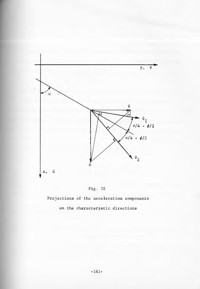
---- T-**y, v
V
*1jt/4 - (zS/2
jt/4 - j>/2
x, u
Fig. 72
Projections of the acceleration components
on the characteristic directions
-141-
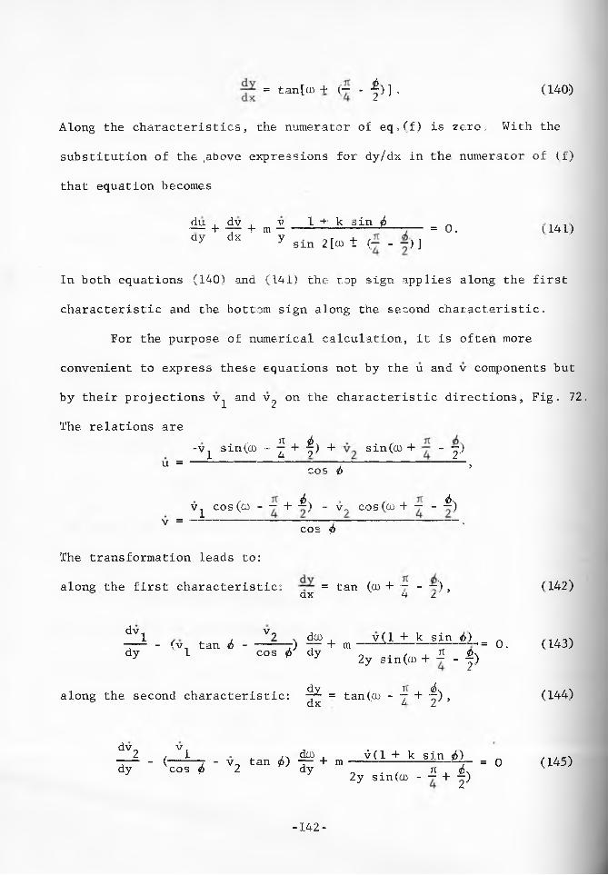
= tan[o) + (~ - -|)] , (140)
Along the characteristics, the numerator of eq.(f) is zero, With the
substitution of the bove expressions for dy/dx in the numerator of (f)
that equation becomes
du , dv , v 1 + k sin fa „—--1- —--b m — — — — ---- --- -— = 0. \141)dy dx y , or„N-i-J J sin 2[u) T (— - — ) ]
In both equations (140) and (141) the top sign applies along the first
characteristic and the bottom sign along the second characteristic.
For the purpose of numerical calculation, it is often more
convenient to express these equations not by the u and v components but
by their projections v^ and v^ on the characteristic directions, Fig. 72.
The relations are”V s i n ( ( D " f + f ) + s i n ( o ) + - -j)
u = --— — — — --- -— —-- — — -— ------ -— — ,cos fa
■ / , fa\ • /' . fa\V^ co s (a) - — + —) - V - co s (co + - - —)V = — - — - — — -------------7— ■— — --- -— ------— •cos fa
The transformation leads to:
along the first characteristic: = tan (to + — - ~) , (142)QX ^ Z
^V1 , V2 v do> , v(l + k sin fa) „ /n/nN-— - (v1 tan fa - — — -t) — + m ---11— - ' • = 0. (143)dy 1 cos fa dy „ . , . rt p,y y 2y sm(a) + - - |)
along the second characteristic: ^ = tan(o> - jr + ^) , (144)
dv v . ,2 / 1 . . da), v(l+ksin«$) _ \-— - (---— t - v tan fa) — + m — -— -— --- ’y- = 0 (145)dy cos fa 2 dy . it fa \ '2y sm(co - - + j)
-142-

It will be noted that the acceleration characteristics, as well as
the stress characteristics, coincide with the slip lines.
Superposition. Since both, the equation of continuity (d) and
isotropy (e), are linear and homogeneous, a linear combination of two
(or more) solutions of an initial acceleration field is also a solution.
Physical conditions.
The physical conditions which need to be applied to incipient
failure are less restrictive than they were for steady state flow.
A. Some, small, tensile (negative) stresses are permissible.
B. A line of infinite shear strain rate may occur along a slip line
or a weak wall.
C. The velocity V of an element of a solid is zero.
D. The acceleration of an element,
dV dV - , V2 -dt dt S p n ’Ms
along the path of its travel, Fig. 18, is bounded. This implies that
dV/dt is bounded but 1/n need not be bounded since V = 0.s
E. Singularities in density are inadmissible.
Grids and special lines.
There is a great deal of similarity between the grids and special
lines of steady state flow and incipient failure. The differences will
be particularly emphasized here. As before, the solution of the stress
field contains the direction of the major pressure a in the differential
form oo = co(x,y) .
1. Sliplines, stress and acceleration characteristics. These three
grids coincide in incipient failure. They form lines inclined at angles
to "t (rt/4 - 6/2) .
2. Lines of maximum shear strain rate. These lines are, of course,
inclined at co "t jt/4 but they are of little significance in incipient
failure since they are not observed.
3. Trajectories. Failure is a time dependent process and, therefore,
paths of travel of the elements will be referred to as trajectories. The
trajectories may have cusps at the initial points, since velocity starts
from zero at those points. This is important, because the stress field
may be bounded by a stress envelope and incipient failure may occur along
a slipline merging into the envelope. This slipline may have a cusp
at the envelope yet become a trajectory.
4. Acceleration discontinuities. A line of acceleration discontinuitj
develops into a line of velocity discontinuity. Such a line has to be
a trajectory (or a streamline) and has to follow a slipline or a weak
wall. It separates two regions which may be both plastic, both rigid
(or elastic), or one plastic and the other rigid (or elastic).
5. A straight acceleration characteristic in plane strain enforces
a constant projection of the acceleration vector on that characteristic.
This is evident from, say, eq. (143).
6. Walls. A wall separates a plastic region from a stationary
rigid (or elastic) region. Usually, there is a velocity discontinuity
-144-

along a wall: the wall then is a streamline and stresses along it are
defined either by the yield locus, for a rough wall, or by the wall yield
locus, for a weak wall. When the solid fails along a rough wall, the
wall is a slipline and a stress and acceleration characteristic. The
coincidence of an acceleration characteristic with a streamline leads to
the relation
V2 ym (l + k sin Cj (146)
along the wall. This relation is readily obtained from, say, eq. (143)
with v^ = V, v2 = V sin */>. Evidently V can be zero along such a wall,
which means that a field can develop without an acceleration discontinuity
along the rough wall.
When the solid fails along a weak wall, equations (79) and (80)
apply along the wall with substituted for 5 , and an acceleration
discontinuity is mandatory since a zero acceleration along the wall
would enforce a zero acceleration within a region of the plastic field.
7. A stress discontinuity may occur only along a trajectory for the
reason given in steady state flow, point 11.
8. Stress singularities are inadmissible for the reason given in
steady state flow, point. 12.
Doming
Consider the pressures acting in a dome which has formed across a
channel of width B, Fig. 73. It is assumed that the dome will fail if
the bottom layer of the dome fails. The bottom layer is taken of a
-145-

unit thickness, measured in the vertical direction. Evidently, the
pressures in the layer are at a minimum when the surface of the dome is
smooth and regular and, barring the possibility of tensions, when the
mass above does not bear down on the layer. The latter implies zero
stress between the layer and the mass above. Under these conditions the
layer can be thought of as a self-supporting dome, geometrically and
stress-wise independent of the vertical coordinate. The major pressure
acts in the plane of the dome.
If the vertical axis of the dome is drawn through its highest point,
then at a distance y from the axis
- 2 T vO- sin 2,to = -— ■— L.1 1 + m
For failure to occur ^ fc, orf
2y ^ (1 + m) sin 2a>. (g)I
For symmetrie channeIs, 2y = B and the largest dome occurs for
cd' = 3^/4 a.nd co" = Jt/4. For such a dome to fail, it is necessary thatf
B > (1 + m) y . (147)
For asymmetric plane strain with one wall vertical, 0*= 0, eq.(g)
gives different relations for each abutment. The conditions on the
sloping wall, 0 = 0 ' , will be denoted by a prime, while the conditions
at the vertical wall will be denoted by the superscript v. The rela
tions for failure at the two abutments are
f1 s i n 2co1 fV s in 2u)V B - a > - ~~f-f-- -— and a > — — — -- (148)
The above formulas (147) and (148) assume that the wall is sufficiently
-146-
Doming
strong to support the major stress at an angle = n/4, for the symmetric
dome, and at angles and tu" for asymmetric plane strain. In view of
the uncertainty of the value of <t>' in incipient failure, these assump
tions appear reasonable and on the safe side.
Piping
The conditions leading to the incipient failure of a solid around
a vertical, circular hole, or pipe is analysed in this section. The
unconfined yield pressure f and the angle of friction are assumed
constant throughout the failing region. The stress field is assumed
axi-symmetric with a traction-free inner boundary of constant diameter
D, Fig. 74.
These assumptions imply independence of the vertical coordinate x
as well as the circumferential coordinate Ci. A relation will be derived
between the yield properties of the solid (fc , ) and the smallest
diameter D at which a bounded plastic field can develop.
The equations of equilibrium (48) and (49) now reduce to
T da a
dy + ycr.a = 0.
Ratio
(149)
is introduced and the equations of equilibrium transform to
(a) Bounded field
Fig. 74
Piping
-149-
da a - a _J£ + ^ L _ dn 2n+ -*r---^ = 0.
The substitution of expressions (30) , (31) , (37) (with k = +1),
and their appropriate derivatives yields
■4 + 2 cot 2co dto - —^7— -jv- dn = 0, a 2n(n-l) 5
■=(1 - sin 5 cos 2co) + 2 sin sin 2oo dco - 4^ sin ^(1 + cos 2co) = 0. a zn
a is now eliminated between these two equations and, after transforma
tion, the following differential equation is obtained.
dm _ JL ___sin 2co , 1 - sin j> cos 2oo 1 + sin Msn'idn 2. cos 2,60 - sin 6 ' n - 1 2n ‘
The solution of this equation produces a family of curves co = cd (n)
Fig. 75, passing through the point (n - 1, 00 = 0). Two types of solutions
are distinguished: (a) bounded fields. The bound of the plastic field
is provided by an envelope of the second family of characteristics.
The envelope occurs for 0) = ic/4 - i/2, and along it dco/dn-*■«*. (b) Un
bounded fields, for which the term within brackets, and with it dco/dn,
change sign for to less than rt/4 - 6/2. The physical field extends
without bound as n increases.
Since the plastic field is independent of the vertical coordinate^
a field (b), unbounded in the horizontal direction, is unbounded in all
directions. Such a field does not represent a real situation and, hence,
only the bounded fields (a) are accepted as solution to piping. The
question is now posed: What is the smallest diameter D at which incipient
-150-
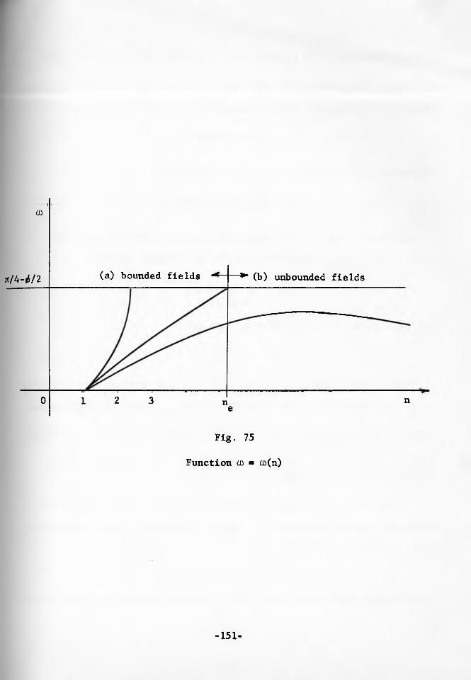
CDJl
jt/4-^/2 (a) bounded fields * (b) unbounded fields
0 1 2 3 n ne
Fig. 75
Function cd ■ co(n)
-151-
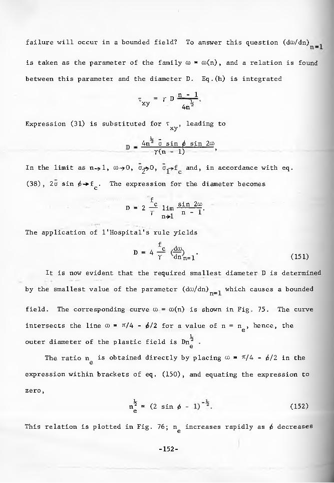
I
failure will occur in a bounded field? To answer this question (dco/dn)
is taken as the parameter of the family co = co(n) , and a relation is found
between this parameter and the diameter D. E q „(h) is integrated
= D n ~ ^V ' r 4n% ‘
Expression (31) is substituted for TXy> leading toi __ 4n a sin j sin 2co
. r(n - 1) ’
In the limit as n-»l, co-?0, a^>0, and, in accordance with eq.
(38), 2a sin $-»fc . The expression for the diameter becomes
f . „„ . . „ c , . s m 2coD = 2 — lim ------7.T . n - 1 n»l
The application of l'Hospital's rule yieldsf , n , c ,do\
° 4 r dn n=l" (151)
It is now evident that the required smallest diameter D is determined
by the smallest value of the parameter (dco/dn)n_^ which causes a bounded
field. The corresponding curve co = co(n) is shown in Fig. 75. The curve
intersects the line co = Jt/4 - i/2 for a value of n = n , hence, theei;outer diameter of the plastic field is Dn .e
The ratio n is obtained directly by placing co = rt/4 - i/2 in the eexpression within brackets of eq. (150), and equating the expression to
zero,
n^ = (2 sin i - (152)e
This relation is plotted in Fig, 76; n^ increases rapidly as <t> decreases
-152-
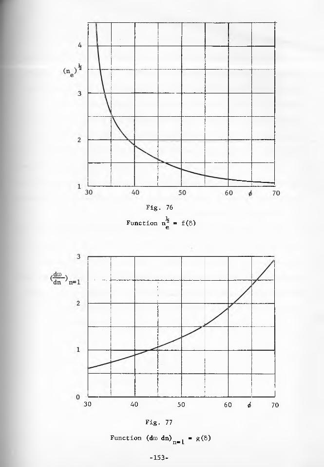
Fig. 76
Function n^ = f(8) e
30 40 50 60 i 70
Fig. 77
Function (do) dn) , = g(6) n = 1
-153-

toward 30° . For fa = 30° , = °°.
Solids whose angle fa approaches the low value of 30° also have low
values of f and stable piping is not observed in these solids. Hence,
the analysis loses its practical value as that value of fa is approached.
However, it is of interest to note that, for values of fa > 19.5°
(sin fa = 1/3), both types of fields, (a) and (b) , exist. For fa < 19.5°,
only type (a) remains, because the expression within brackets of eq.
(150) does not change sign and dco/dn is positive for all values of n > 1.
Values of (dco/dn) , for the smallest diameter D at which incipient n—1failure must occur in a bounded field have been computed numerically and
are plotted in Fig. 77. The diameter D is then obtained for any material
of known ratio f /T from eq.(151). cIt is interesting to note that investigations of slope stability in
axial symmetry [22] lead to profiles which all converge to a vertical
hole, Fig. 78. Within the accuracy of numerical calculations, the
diameter of that hole seems to be independent of the starting diameter at
the surface and seems to equal D, the diameter computed above for the
smallest bounded field independent of the vertical coordinate.
An acceleration field for piping is given in reference [22].
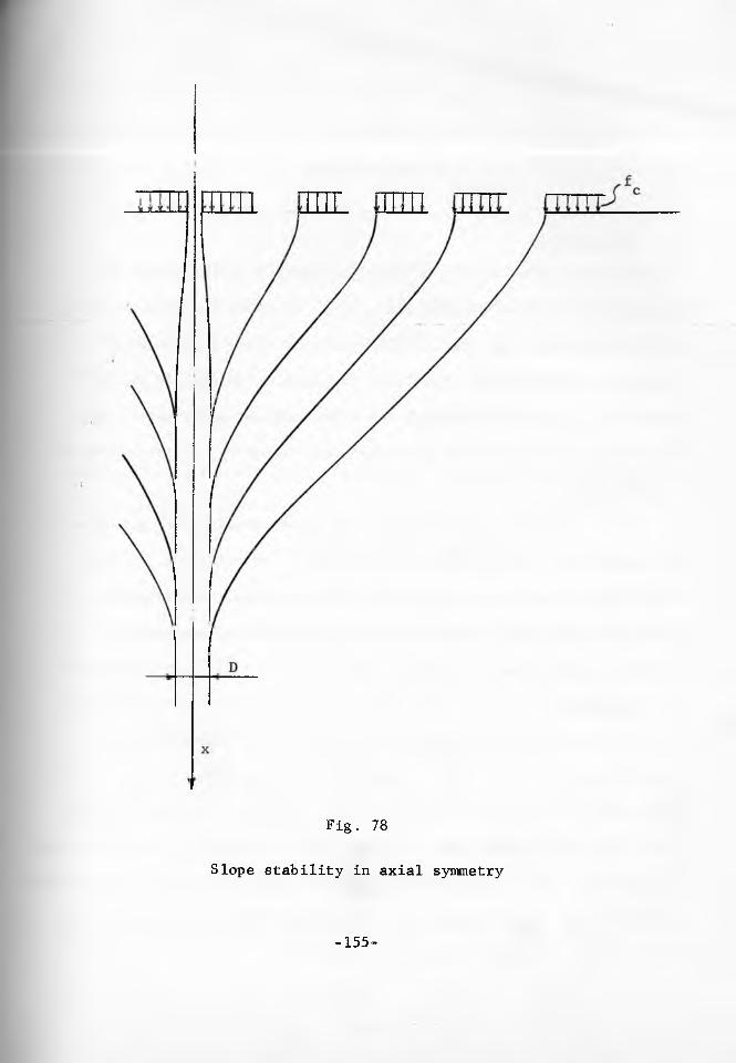
Fig..78
Slope stability in axial symmetry
-155-

PART IV
FLOW CRITERIA
Introduction
The flow of a solid in a converging channel is subject to two
typical obstructions: doming and piping. The flow criteria are based
on the assumption that the solid consolidates under the pressures
prevailing during steady state flow, develops an unconfined yield
pressure f^, in accordance with its flow-function, and flows if the
unconfined yield pressure is insufficient to support a stable dome or
a stable pipe.
Thus, the flow criteria relate the major consolidating pressure
of steady state flow with the pressures of incipient failure,
defining minimum ratios a- /£ ~ called critical flow-f actors,
which the solid must exceed for flow to start and to continue.
No-doming
Doming usually originates at the outlet of a channel where a
radial stress field is closely approached during flow, and that field
is assumed in the derivation of the flow criteria. The dome formulas
(147) and (148) contain the unconfined yield pressure f at the abutments
of the dome, i.e. at the end points of the walls. The major consolidating
pressure is given by eq. (20) . With substitution (102) for cr in
radial flow, the major pressure at a wall is
-156-

cr | = r x s(0')(l + sin 5).
a| is eliminated by means of the flowfactor ff, eq,(41) thus
ff = r s(0') (1 + sin 5) . (a)c
Plane and axial symmetry, A channel, Fig. 79 (a), is symmetric
for the purpose of this analysis if its walls are symmetric with respect
to the vertical axis in the neighborhood of the vertex, hence, -0" =0',
Then, from the figure, r = B/2 sin 0' and eq.(a) becomes
_ _ B_j s (01)(1 + sin S)i t ” r o • r 1 *f 2 sin 0c
Substitution for B y/f^ from the eq.(147) produces the following value
of the critical flowfactor
ff (153)2 sin 0
This is the no-doming formula for symmetric channels.
For the particular case of vertical chanels, 0' = 0" = 0, an
expression for the flowfactor is obtained in a closed form by substitut
ing expression (126) for a in eq. (20), thus
a = .. r y (1 + sin 5) ^1 (1 + m) sin 5 sin 2CO
is eliminated by means of eq,(41) and, since at a wall y = y 1 = -B/2,
the expression for the flowfactor becomes
B x ________1 + sin 5_____________ff = f 2(1 + m) sin 6 sin (2co' - rt)
Substitution for By/f from the eq.(147) yields
-157-
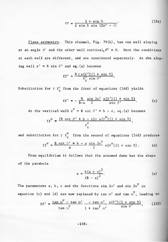
££ _ ______1 + sin S . (154)2 sin 6 sin (2031 - it)
Plane asymmetry. This channel, Fig. 79(b), has one wall sloping
at an angle 0' and the other wall vertical,0" = 0. Here the conditions
at each wall are different, and are considered separately. At the slop
ing wall r 1 = B sin 0' and eq.(a) becomes
ffi - BT s ( 0 ')(1 + sin 5)“ f' sin 0' ‘c
Substitution for y f^ from the first of equations (148) yields
B sin 2co' s(0')(l + sin 5) , sff = " B^a 2 sin 0' * (c)
At the vertical wall rV = B cot 0' + b - c, eq„(a) becomes
ffv «. (B cot 0' + b - c)r s(0V)(l + sin 5)fV ’ c
and substitution for y f^ from the second of equations (148) produces
r f~v B cot 0' + b - c sin 2coV ,„vv ,, . . ^f f = ------------------ — ----- s (0 ;(1 + sin 8). (d)a I
From equilibrium it follows that the assumed dome has the shape
of the parabola?b (a + y) / \x = — ----- (e)
(B - a)
The parameters a, b, c and the functions sin 2o>' and sin 203V in
equation (c) and (d) are now replaced by tan 03' and tan 03V , leading to
ff i _ tan coV - tan Q)1 - tan Q31 s (0 ') (1 + sin 5)f ,,sv , 2 , sin 0' ’ Ktan 03 1 + tan 03'
-158-

(a)
(b)
Fig. 79
Outlet conditions for no doming
-159-
„„v (tan co1 - tan cov ) ( 2 cot 0 ' tan co' tan oov - tan ojV - tan c o ' )ff = ---------------------------------------------------------------Sc2 tan os'(1 + tan co )
x s(0V)(1 + sin 5). (156)
The acceptable range for angle (jo' is 3fl/4 < co' < i t . Within this range
dffV/cko' > 0, while c i f f ' / c k o ' < 0, and there is one value of co' for
which ffV = ff' = ff. This value of the flowfactor is maximized with vrespect to co , yielding the critical flowfactor.
Flowfactor plots. Contours of constant values of the critical
flowfactors are plotted for 6 = 30°, 40°, 50°, 60° and 70° for plane
symmetry in Figures 80 to 84, and for axial symmetry in Figures 85
to 89. For plane asymmetry, the flowfactor is plotted in Figures 90
to 92 for 5 = 50° and for an angle of friction at the vertical wall
0V = 20°, 30°, and 40°.
Influence of compressibility. Figures 93 and 94 show a comparison
of the flowfactors for a compressible solid with P = 0.10, with those
of an incompressible solid. The plots are for 5 = 50°. Figure 93
shows symmetric plane strain, and Figure 94 axial symmetry. The contin
uous lines are for the compressible solid, and the dashed lines for
the incompressible solid. The latter are copied from Figures 82 and 87.
It is evident that even the large degree of compressibility corresp
onding to (3 = 0.10 does not appreciably affect the no-doming criterium.
Hence, the compressibility of the solids may be neglected.
-160-
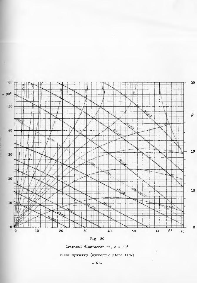
30
20
10
20 30 40 50Fig . 80
Critical flowfactor ff, S = 30°
Plane symmetry (symmetric plane flow)
-161-
60 d 1 70
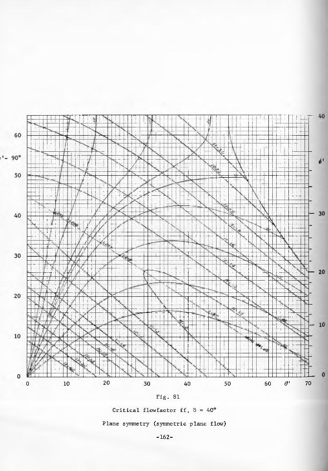
0 10 20 30 40 50 60 &' 70
Fig. 81
Critical flowfactor ff, 8 = 40°
Plane symmetry (symmetric plane flow)
-162-

70
. 90°
60
50
40
30
20
10
0 E
50
40
30
- 20
— 10
30 Fig. 82
Critical flowfactor ff, 5 = 50°
Plane symmetry (symmetric plane flow)
-163-
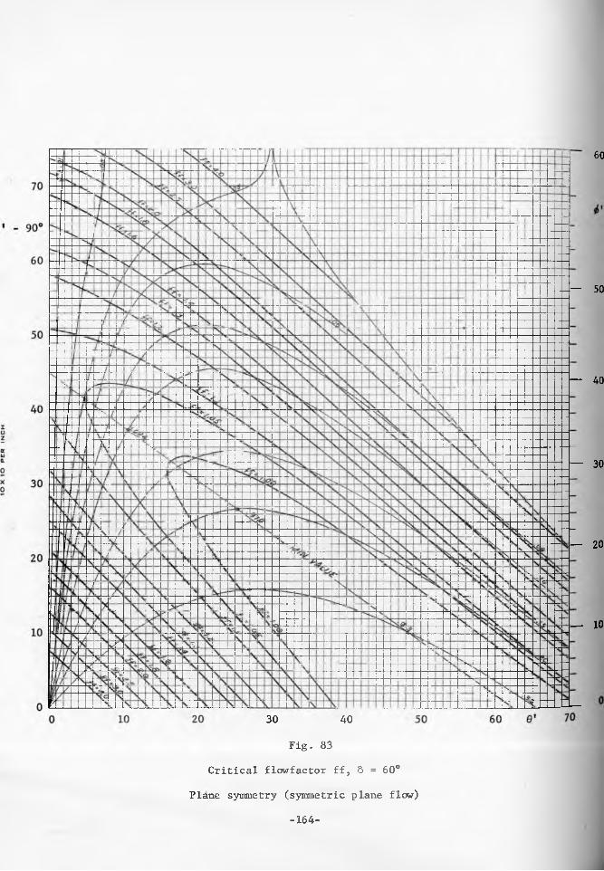
60
— 50
40
— 30
— 20
— 10
30 40
Fig. 83
Critical flowfactor ff, S = 60°
Plane symmetry (symmetric plane flow)
-164-
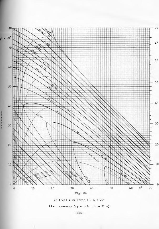
Critical flowfactor ff, 6 = 70°
Plane symmetry (symmetric plane flow)

Fig. 85
Critical flowfactor ff, 5 * 30°
Axial symmetry (conical flow)
-166-

50
90°
40
30
20
10
10 20 30 40Fig. 86
Critical flowfactor ff, 8 = 40°
Axial symmetry (conical flow)
-167-
50 60 0' 70
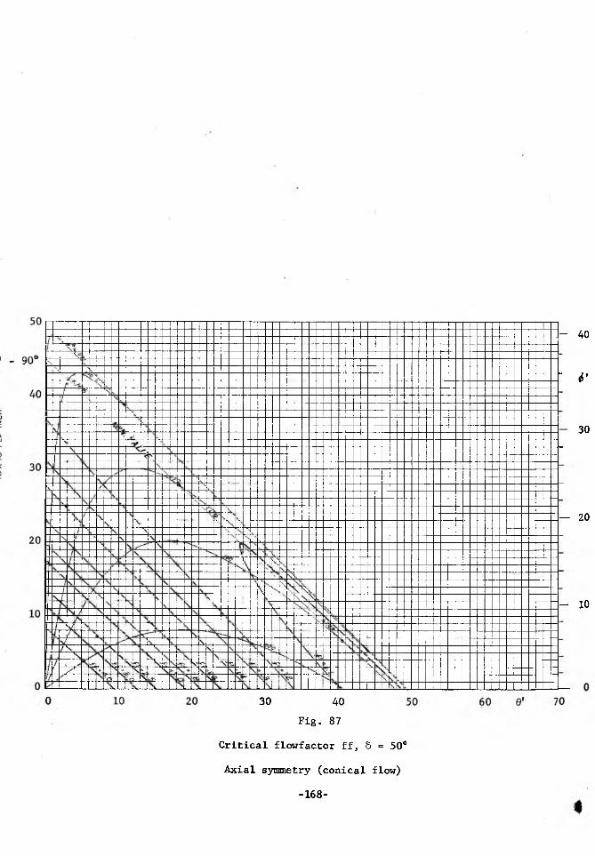
30 40Fig. 87
Critical flowfactor ff, S = 50°
Axial symmetry (conical flow)
-168-
- 40
i'
- 30
— 20
- 10

Fig. 88
Critical flowfactor ff, 6 = 60°
Axial symmetry (conical flow)
-169-
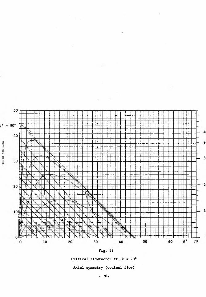
Fig. 89Critical flowfactor ff, 5 = 70°
Axial symmetry (conical flow)
-170-
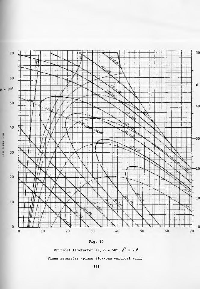
Fig. 90
Critical flowfactor ff, 5 = 50°, = 20°
Plane asymmetry (plane flow-one vertical wall)
-171-

Fig. 91
Critical flowfactor ff, 5 = 50°, 6V = 30°
Plane asymmetry (plane flow-one vertical wall)
-172-

Fig. 92
Critical flowfactor ff, 8 = 50°, = 40°
Plane asymmetry (plane flow-one vertical wall)
-173-
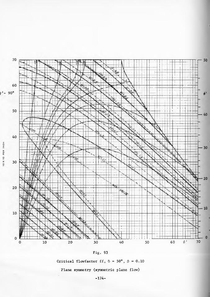
10 20 30 40 50 60 0' 70
Fig. 93
Critical flowfactor ff, 5 = 50°, p = 0.10
Plane symmetry (symmetric plane flow)
-174-
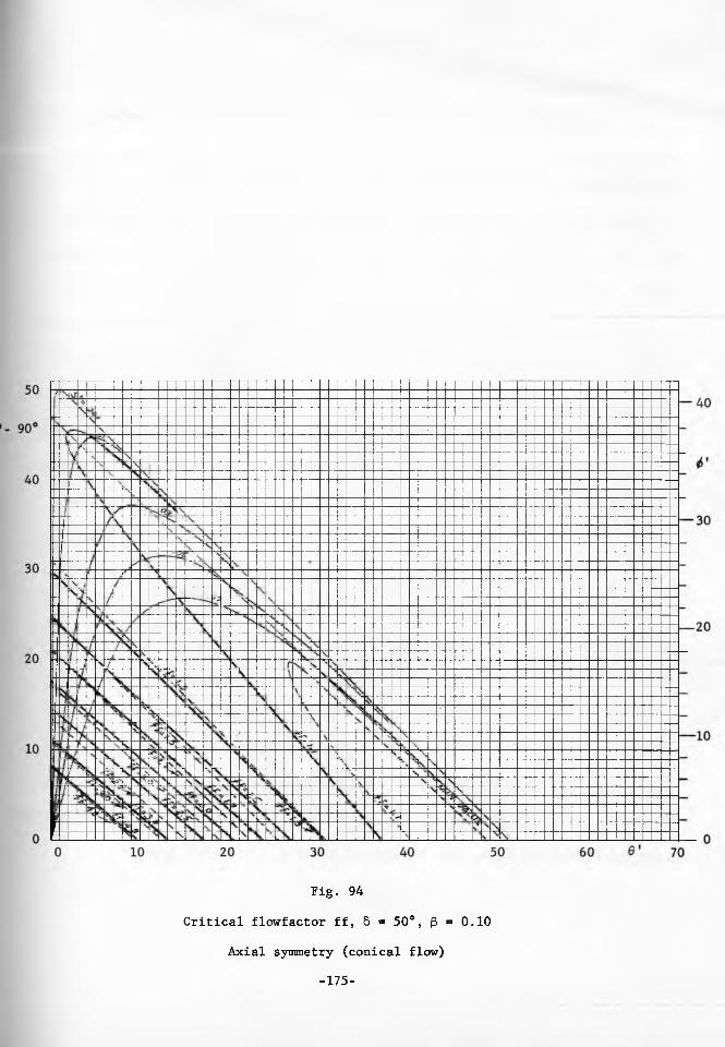
Fig. 94Critical flowfactor ff, 5 <* 50°, p = 0.10
Axial symmetry (conical flow)-175-

No-piping
A tendency for piping exists in all channels in which the solid flows
within rough walls. It was shown in the analysis of axi-symmetric radial
stress fields that such channels are very steep or, indeed, vertical. It
is observed in experiments that these channels circumscribe the outlet
and, hence, that the largest dimension of the outlet defines the diameter
of the channel.
In the derivation of the formula for no-piping it is assumed that the
values of the unconfined yield pressure fc> and of the angle of friction </
are constant throughout the plastic region, Fig. 74 (a). The values dev
eloped at the inner surface of the pipe are assumed to prevail throughout
the region. These assumptions are reasonable, because the plastic regionj.is quite thin (see ratio n*, Fig. 76) for the solids with large angles
of friction, i.e. for the solids which have the greatest tendency to
pipe. In selecting the value of f it is necessary to use the time flow-
function because, while the solid is flowing within the pipe, outside
the pipe the solid is consolidating at rest. The angle of friction <t> -
which exists at a traction-free, inner surface, is measured at the point
of tangency of the time yield locus with the f circle, Fig. 95.
The unconfined yield pressure f at the inner surface of the pipe
is assumed to be generated by the major pressure a"^ due to steady state
flow in a vertical channel of diameter D. This pressure is given by eq.(20)
with substitution (126) for a, and with y = D/2, go = to", thus
n" = D r(l + sin 5) m1 4 sin 5 sin 2co"' v ;
-176-
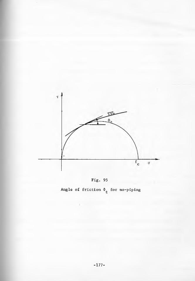
Fig. 95
Angle of friction $ for no-piping
-177-
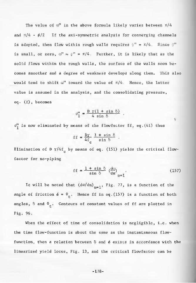
The value of to" in the above formula likely varies between it/4
and jt/4 - fa/2 If the axi-symmetric analysis for converging channels
is adopted, then flow within rough walls requires \|r" = it/4. Since 0"
is small, or zero, to" as \|/" = rt/4. Further, it is likely that as the
solid flows within the rough walls, the surface of the walls soon be
comes smoother and a degree of weakness develops along them. This also
would tend to shift to" toward the value of rt/4. Hence, the latter
value is assumed in the analysis, and the consolidating pressure,
eq. (f), becomes
When the effect of time of consolidation is negligible, i.e. when
the time flow-function is about the same as the instantaneous flow-
function, then a relation between 5 and 6 exists in accordance, with the
linearized yield locus, Fig. 13, and the critical flowfactor can be
cr” is now eliminated by means of the flowfactor ff, eq„ (41) thus
Df 1 + sin S 4f sin 5c
Elimination of D V/4f by means of eq. (151) yields the critical flow
factor for no-piping
sin 5 dn© (157)n=l
It will be noted that (dto/dn)n_^. Fig. 77, is a function of the
angle of friction 6 = $ . Hence ff in eq„(157) is a function of both
angles, 5 and $ . Contours of constant values of ff are plotted in
Fig. 96.
-178-
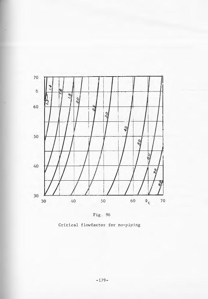
30 40 50 60 3>r 70
Fig. 96
Critical flowfactor for no-piping
-179-
computed as a function of angle 5 only. In this case
a, = a, and a = a + f (1 - sin i ) !2 sin &.I I c
From equation (20) and (35)cr, a + f (1 - sin {6)/2 sin 6I , - 1 c
0 = T ~T — : S' a n d a = -------- --------t— t— ~ — ---------------- ------- ,1 + s m o 1 + sin ®
Elimination of a and a by means of the above equations, and of the ratio
cr^/fc by means of the flowfactor ff, in accordance with eq„(41), yields
• r _ 2 ff sin <h + 1 - sin <£>Sin 2 ff - 1 + sin £ ° (g)
Elimination of sin 5 in eq„(157) produces
_ 1 + sin j dax 1 - sinsin 6 dn . 2 sin & ° n= 1
ff is computed as a function of <j> from this equation, then 5 is computed
as a function of & from eq„(g). Angle 6 is eliminated, yielding the
function ff(S) which is plotted in Fig. 97. It is noticed that piping
does not occur in solids which are not affected by consolidation at rest,
and whose 5 < 54.5°.
A comparison of the flowfactor values for no-doming and no-piping
shows that piping is much more apt to occur and more difficult to avoid
than doming. In fact, solids which gain a significant amount of
strength with consolidation at rest invariably tend to pipe.
-180-

Fig „ 97
Critical flowfactor for no-piping for
solids not affected by consolidation at rest
-181-

PART V
TESTING THE FLOW PROPERTIES OF BULK SOLIDS
Apparatus
The solids considered in this work include soils. Since the field ..
of soil mechanics was well developed at the time when this study-
originated (1952), it was natural first to investigate the applicability
of the soil mechanics testing apparatus to the measurement of the flow
properties of bulk solids.
Standard direct shear apparatus and unconfined compression apparatus
were tried. The results obtained with shear apparatus were not satis
factory, primarily, because the range of values of cohesion for which
the soil test machines were designed was outside the useful range for
bulk solids. By the terminology of soil mechanics, bulk solids can be
considered cohesionless, and cohesive soils under their usual degree of
consolidation would not flow by gravity in any storage system. Un
confined compression apparatus was found unsuitable because of the
impossibility of applying a known, uniform consolidation, and because
the stresses due to the weight of the sample were in the range of the
measured yield stresses. These samples often disintegrated during
handling. The application of a triaxial compression apparatus was con
sidered and rejected as impractical because of the considerable time
required to obtain results by this method. It was decided to develop
a machine especially for testing bulk solids.
A direct shear test machine was designed and built in 1953. It has
-182-
since undergone many refinements; the type now in use in the USA and in England is shown in Fig. 98. It is equipped with a shear cell, a gravity
vertical loading system, and an electric-pneumatic shearing force device.
The shearing force device has a constant strain-rate of 0.036 in. per min.
The shearing force necessary to maintain the strain-rate is continuously
recorded on a pneumatic recorder. This arrangement produces a permanent
record of the stress-strain relations for each test. A test cell is
shown in Fig. 99. It is composed of a base located on the frame of the
machine, a ring resting on top of the base, and a cover. The bottom
of the cover and the inside of the base are roughened to increase
adhesion of the tested solid. The base and the ring are filled with
the tested solid. The vertical compressive force V is applied to the
cover. The horizontal shearing force S is applied by means of a stem
which acts on a bracket attached to the cover. The stem acts in the plane
of contact between the ring and the base. A part of the shearing force
is tranferred from the bracket to the ring through a loading pin.
The difference between the inside diameter of the ring and the outside
diameter of the cover is 0.04 in.
Shear cells are used in two sizes: 2.5 and 3.75 inches inside
diameter. The smaller cell is used for heavy solids like ores, while
the larger cell is preferred for light solids. The machine is capable
of applying a vertical force up to 100 lb and a shearing force up to
60 lb.
The shear test machine is used in conjunction with a six cell con
solidating bench in which the whole cells are placed for the time of
consolidation at rest, Fig. 100.
-183-

Fig. 98
Direct shear apparatus
-184-
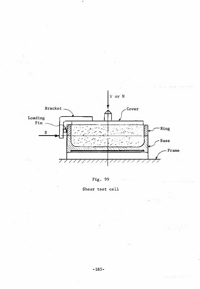
Fig. 99
Shear test cell
-185-

Testing
The purpose of the tests is to measure the flow properties of a
solid (5 and flow-function), its density, and the angle of friction <t>'
between the solid and a sample of the wall. The flow properties are
measured for two consolidating conditions: the condition of continuous
flow, and the time effect of consolidation at rest after flow has stopped
and material is left under pressure. Density and the angle of friction
<t>' are measured for continuous flow only.
The tests give significant results provided the procedure is such
as to assure: (a) a representative specimen, (b) a uniform specimen,
and provided that the stresses occurring during (c) flow, and (d)
shear are known with sufficient accuracy. While these requirements sound
commonplace, they are by no means easy to satisfy. Both the apparatus
and the procedure described herein are the result of extensive
experimentation. It is believed that the described method has brought
the errors of tests within the range of scatter inherent in bulk
solids flowing in a channel.
Continuous flow
(a) Representative specimen. In general, the yield locus of a
solid for a given consolidating pressure and given strain-rate is
affected by the water content, temperature, and particle size distribu
tion of the specimen. The tests are conducted on solids containing water
below the point of saturation. In view of the considerable influence
which water content has on the yield loci of many materials it is
-186-

Fig. 100
Consolidating bench
-187-
necessary to reproduce the required content in the specimen accurately
and to handle the specimen rapidly so as to minimize errors through
evaporation,
When temperature is a significant factor, the solid and the con
solidating bench are placed in a heated chamber, Fig. 101. The tests
are carried out when the solid has reached the required temperature.
The particle size distribution is not as perplexing as it might
appear at first sight. In the flow of bulk solids, the interest lies
in the conditions that lead to stoppages of flow, which it is necessary
to avoid. Stoppages occur when the solid reaches a sufficiently high
yield strength. Thus, the critical conditions to be considered are
those of highest strength. During the flow of a mass of mixed particle
sizes, the large particles move bodily while the material shears across
the fines. Therefore, the yield strength of the mass depends on the
properties of the fines. The coarse particles are a passive agent
and like aggregate in concrete they do not develop yield strength
without fines to bind them. Experience shows that screened out coarse
ores in bulk are invariably free flowing; they do not develop any
cohesion. To determine the yield loci of a mixed material, the fines
are screened out through an arbitrarily chosen No. 20 mesh (0.033 in.
aperture) sieve and tested.
(b) Uniform specimen. The consolidation of the sample is carried
out in two stages. The purpose of the first stage is the preconsolida
tion of a uniform specimen. With the cover off the test cell, a packing
mold is placed on top of the ring and both the mold and the ring are
-188-

placed in an offset position on the base, as shown in Fig. 102. A
specimen of the tested solid is then placed in the cell. One layer after
another is slightly packed with the fingers, up to the top of the mold.
The excess material is scraped off level with the top of the mold. A
twisting top is placed over the specimen. The top is essentially like the
cover of Fig. 99 but with a smooth bottom surface and without the bracket.
A vertical force V is applied to the top by means of the system of lever
and weight shown in Fig. 98. Force V causes a vertical pressure cr in
the material. By means of a special wrench, an oscillating twist is
now applied to the cover. This preconsolidates the solid and assures
a uniform specimen.
(e) Flow. Consolidation is completed by causing the specimen to
flow under given stresses until a steady state is closely approached.
This is attained in the following way: Load V is released, the twisting
top and the mold are removed, the excess material is scraped off level
with the top of the ringyand the test cover is placed on the material.
Load V is now replaced and a shearing force S is applied to the bracket,
Fig. 103, by means of the electric-pneumatic shearing device. The shear
ing force is distributed between the cover and the ring.
This method of applying the shearing force seems to assure a fairly
uniform distribution of the stresses across the specimen, Prior to the
adoption of this method, the shearing force used to be applied directly
to the ring. This would cause distinct stress concentration at the
loaded edges of the ring and of the base. Material in. the ring would
-190-
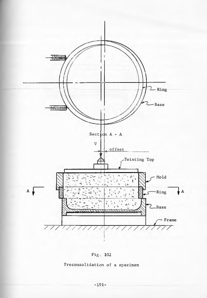
Fig, 102
Preconsolidation of a specimen
-191-
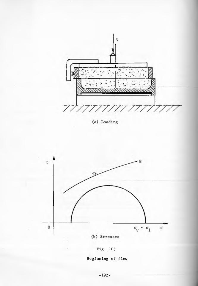
V
Fig. 103
Beginning of flow
-192-
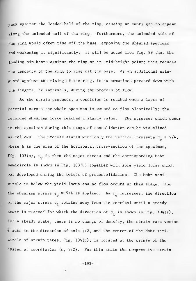
pack against the loaded half of the ring, causing an empty gap to appear
along the unloaded half of the ring. Furthermore, the unloaded side of
the ring would often rise off the base, exposing the sheared specimen
and weakening it significantly. It will be noted from Fig. 99 that the
loading pin bears against the ring at its mid-height point; this reduces
the tendency of the ring to rise off the base. As an additional safe
guard against the rising of the ring, it is sometimes pressed down with
the fingers, at intervals, during the process of flow.
As the strain proceeds, a condition is reached when a layer of
material across the whole specimen is caused to flow plastically; the
recorded shearing force reaches a steady value. The stresses which occur
in the specimen during this stage of consolidation can be visualized
as follows: the process starts with only the vertical pressure cr = V/A,
where A is the area of the horizontal cross-section of the specimen,
Fig. 103(a), cr is then the major stress and the corresponding Mohr
semicircle is shown in Fig. 103(b) together with some yield locus which
was developed during the twists of preconsolidation. The Mohr semi
circle is below the yield locus and no flow occurs at this stage. Now
the. shearing stress = S/A is applied. As increases, the direction
of the major stress rotates away from the vertical until a steady
state is reached for which the direction of is shown, in Fig. 104(a).
For a steady state, there is no change of density, the strain rate vector
e acts in the direction of axis r/2, and the center of the Mohr semi
circle of strain rates, Fig. 104(b), is located at the origin of the
system of coordinates (e, t /2). For this state the compressive strain
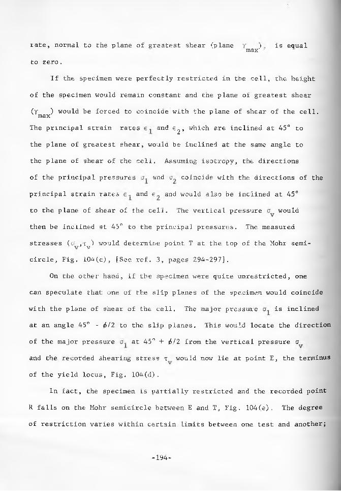
rate, normal to the plane of greatest shear (plane r ). is equalmax'to zero.
If the specimen were perfectly restricted in the cell, the height
of the specimen would remain constant and the plane of greatest shear
(y ) would be forced to coincide with the plane of shear of the cell, maxThe principal strain rates and e^, which are inclined at 45° to
the plane of greatest shear, would be inclined at the same angle to
the plane of shear of the cell. Assuming isotropy, the directions
of the principal pressures and cr coincide with the directions of the
principal strain rates and e and would also be inclined at 45°
to the plane of shear of the cell. The vertical pressure would
then be inclined at 45° to the principal pressures. The measured
stresses (cr ,tv) would determine point T at the top of the Mohr semi
circle, Fig. 104(c), [See ref. 3, pages 2.94-297].
On the other hand, if the specimen were quite unrestricted, one
can speculate that one of the slip planes of the specimen would coincide
with the plane of shear of the cell. The major pressure is inclined
at an angle 45° - <t>!2 to the slip planes. This would locate the direction
of the major pressure at 45° + <t>/2 from the vertical pressure a
and the recorded shearing stress -r would now lie at point E, the terminus
of the yield locus, Fig. 10i(d).
In fact, the specimen is partially restricted and the recorded point
R falls on the Mohr semicircle between E and T, Fig, 104(e), The degree
of restriction varies within certain limits between one test and another;
-194-
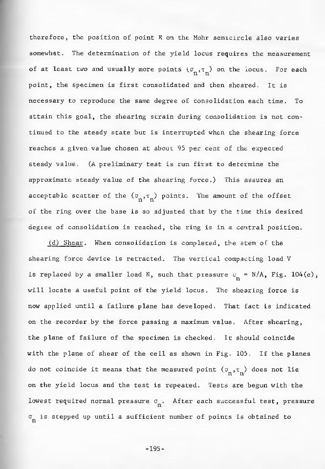
therefore, the position of point R on the Mohr semicircle also varies
somewhat. The determination of the yield locus requires the measurement
of at least two and usually more points (a ,t ) on the locus. For eachn npoint, the specimen is first consolidated and then sheared. It is
necessary to reproduce the same degree of consolidation each time. To
attain this goal, the shearing strain during consolidation is not con
tinued to the steady state but is interrupted when the shearing force
reaches a given value chosen at about 95 per cent of the expected
steady value, (A preliminary test is run first to determine the
approximate steady value of the shearing force.) This assures an
acceptable scatter of the (an JTn) points. The amount of the offset
of the ring over the base is so adjusted that by the time this desired
degree of consolidation is reached, the ring is in a central position.
(d) Shear. When consolidation is completed, the stem of the
shearing force device is retracted. The vertical compacting load V
is replaced by a smaller load N, such that pressure Un = N/A, Fig. 104(e),
will locate, a useful point of the yield locus. The shearing force is
now applied until a failure plane has developed, That fact is indicated
on the recorder by the force passing a maximum value. After shearing,
the plane of failure of the specimen is checked. It should coincide
with the plane of shear of the cell as shown in Fig, 105. If the planes
do not coincide it means that the measured point (a ) does not lier n non the yield locus and the test is repeated. Tests are begun with the
lowest required normal pressure a . After each successful test, pressure
is stepped up until a sufficient number of points is obtained to
-195-

(b) Strain rate Mohr circle
Fig. 104
Steady state flow
-196-
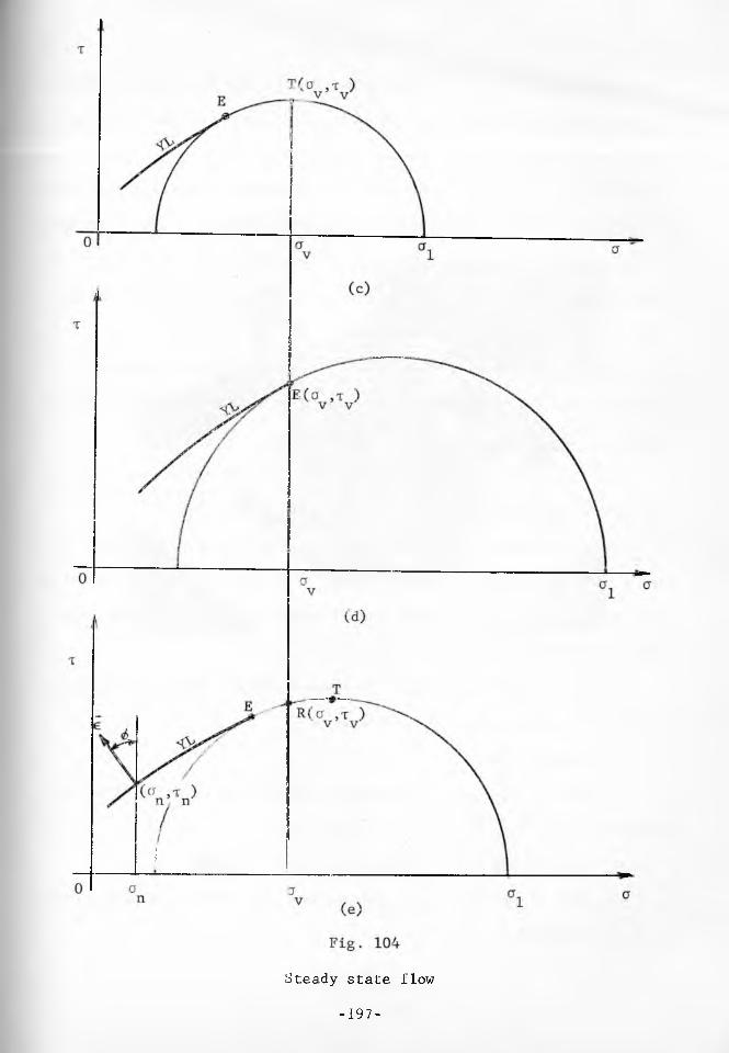
Steady state flow
-197-
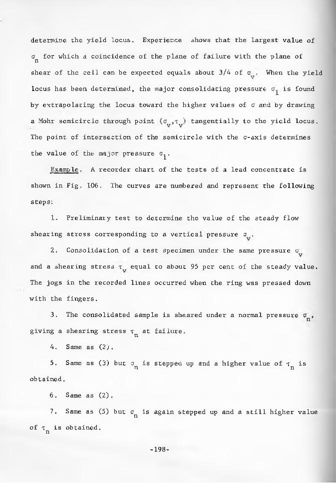
determine the yield locus. Experience shows chat the largest value of
a for which a coincidence of the plane of failure with the. plane of nshear of the cell can be expected equals about 3/4 of a . When the yield
locus has been determined, the major consolidating pressure is found
by extrapolating the locus toward the higher values of a and by drawing
a Mohr semicircle through point tangentially to the yield locus.
The point of intersection of the semicircle with the a-axis determines
the value of the major pressure o^.
Example. A recorder chart of the tests of a lead concentrate is
shown in Fig. 106. The curves are numbered and represent the following
steps:
1. Preliminary test to determine the value of the steady flow
shearing stress corresponding to a vertical pressure a .
2. Consolidation of a test specimen under the same pressure cr
and a shearing stress equal co about 95 per cent of the steady value.
The jogs in the recorded lines occurred when the ring was pressed down
with the fingers.
3. The consolidated sample is sheared under a normal pressure
giving a shearing stress Tn at failure.
4. Same as (2).
5. Same as (3) but cr is stepped up and a higher value of Tn is
obtained.
6. Same as (2) .
7. Same as (5) but an is again stepped up and a still higher value
of t is obtained, n
-198-

Fig. 105
Plane of failure of a specimen
-199-
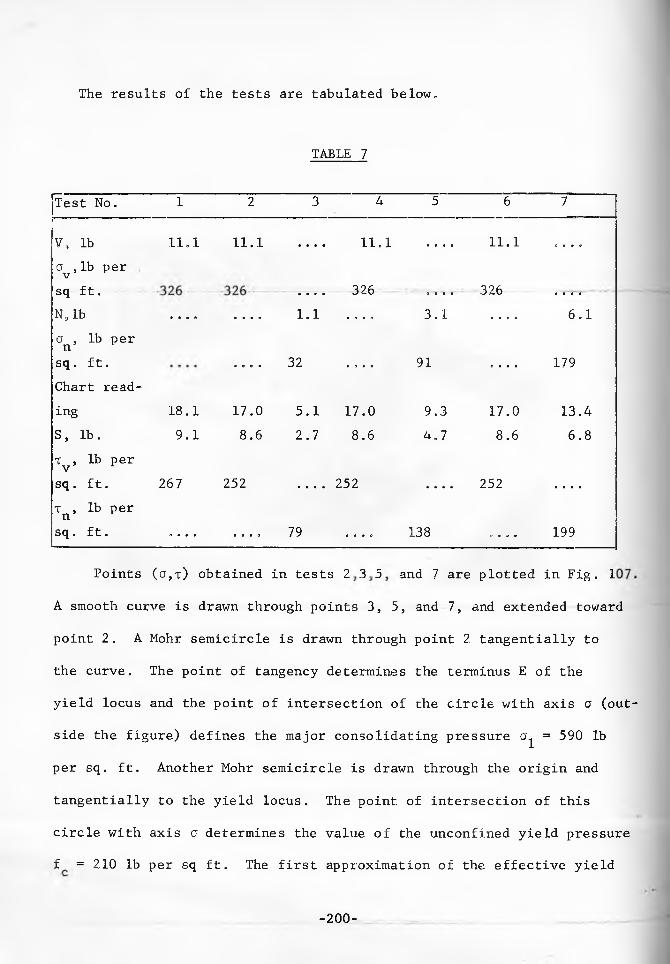
The results of the tests are tabulated below.
TABLE 7
Test No. 1 2 3 4 5 6 7
V, lb 11.1 11.1 • • • • 11.1 • • 9 0 11.1 O • • 9
a , lb perVsq ft. 326 326• • • ■ ....9 * * 0 • • • •
N, lb . . . . • a • a 1.1 • 0 • 0 3.1 o . . . 6.1a , lb per nsq . f t . . . . . 32 . 9 . 0 91 . . . . 179Chart reading 18.1 17.0 5.1 17.0 9.3 17.0 13.4S, lb. 9.1 8.6 2.7 8.6 4.7 8.6 6.8T , lb per v rsq . ft. 267 252 . . . . 252 . . . . 252 . . . .
T , lb per nsq . ft. . . . . . . . . 79 . . . . 138 . . . . 199
Points (a,t ) obtained in tests 2 3 5 and 7 are plotted in Fig . 1
A smooth curve is drawn through points 3, 5, and 7, and extended toward
point 2. A Mohr semicircle is drawn through point 2 tangentially to
the curve. The. point of tangency determines the terminus E of the
yield locus and the point of intersection of che circle with axis a (out
side the figure) defines the major consolidating pressure cr = 590 lb
per sq. ft. Another Mohr semicircle is drawn through, the origin and
tangentially to the yield locus. The point of intersection of this
circle with axis a determines the value of the unconfined yield pressure
f = 210 lb per sq ft. The first approximation of the effective yield
-200-
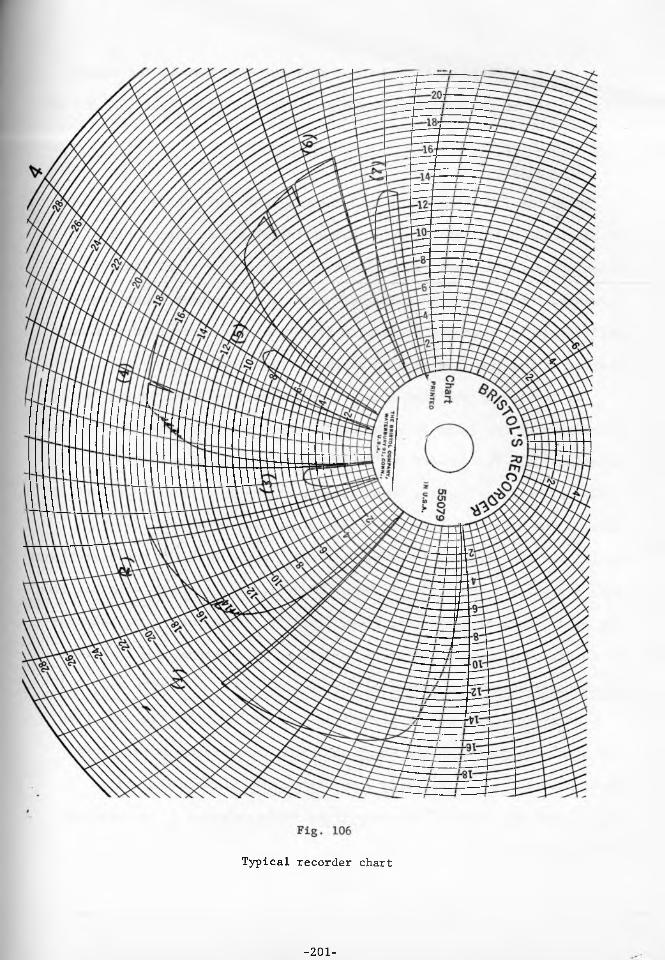
Typical recorder chart
-201-
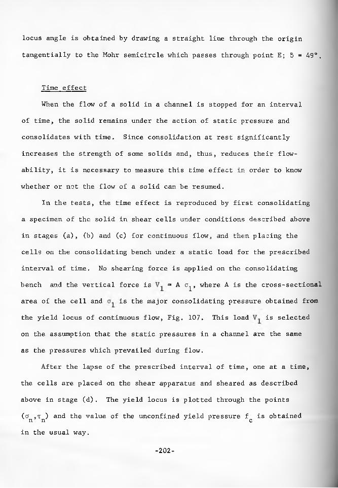
locus angle is obtained by drawing a straight line through the origin
tangentially to the Mohr semicircle which passes through point E; 5 = 49°.
Time effect
When the flow of a solid in a channel is stopped for an interval
of time, the solid remains under the action of static pressure and
consolidates with time. Since consolidation at rest significantly
increases the strength of some solids and, thus, reduces their flow-
ability, it is necessary to measure this time effect in order to know
whether or not the flow of a solid can be resumed.
In the tests, the time effect is reproduced by first consolidating
a specimen of the solid in shear cells under conditions described above
in stages (a), (b) and (c) for continuous flow, and then placing the
cells on the consolidating bench under a static load for the prescribed
interval of time. No shearing force is applied on the consolidating
bench and the vertical force is = A cr , where A is the cross-sectional
area of the cell and is the major consolidating pressure obtained from
the yield locus of continuous flow, Fig. 107. This load is selected
on the assumption that the static pressures in a channel are the same
as the pressures which prevailed during flow.
After the lapse of the prescribed interval of time, one at a time,
the cells are placed on the shear apparatus and sheared as described
above in stage (d). The yield locus is plotted through the points
(a ) and the value of the unconfined yield pressure f is obtained n n J r cin the usual way.
-202-

Construction of a yield locus
-203-

During the static compaction it is necessary to preserve the mois
ture content of the specimen. This is down by covering the shear cells
with plastic cups shown in Fig. 100; the bases of the cups are sealed
by baths of a sealing liquid. When the tests are to be carried out at
an elevated temperature, the consolidating bench is placed in a heated,
thermostatically controlled chamber, Fig. 101.
Density
Since the analysis shows that the influence of the compressibility
of a solid (change of density with consolidating pressure) on the process
of flow is negligible, it is not necessary to obtain a very accurate
function of density versus pressure. However, the density of a solid at
the outlet of a channel, or at the inner surface of a pipe enters the
flow formulas and, hence, needs to be obtained.
The easiest way to measure the density is to weigh the whole cell
after it has been sheared (section (d) above), subtract the weight of
the cell itself and divide the net weight by the volume of the cell.
Plots of the flow properties
For design purposes, f^, y, and 5 are plotted as a function of the
major consolidating pressure cr , as shown in Fig. 108. As will be shown in
Part VI, these plots are very convenient in determining the actual value
of angle 5 and density y which occur at the outlet of a channel or the
inner surface of a pipe.
-204-
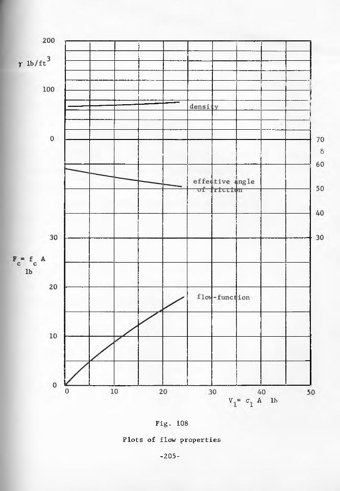
V = a A lb
Fig. 108
Plots of flow properties
-205-

V = a A lb
Fig. 108
Plots of flow properties
-205-

Angle of friction j.1
The angle of friction o' between a solid and a material of the wall
is measured on the direct shear apparatus, Fig. 98, The arrangement of
the cell is shown in Fig. 109. In this case, the base is replaced by
a filler covered with a specimen of the material of the wall, the ring
is placed over it, filled with the solid, and enclosed with the cover.
All the tests necessary to determine angle ' are now run without
replacing the solid. The procedure is as follows: the smallest vertical
load V is placed and the shear foce S is applied until a steady reading
is obtained. The stem is then retracted, the load V is increased and
the force S is again applied until a steady value is reached. This
precess is repeated for the required range of loads V. After the highest
load V has been run, some solid is added to the cell so that the level
of the solid in the ring is flush with the cop of the ring, This is
done without disturbing the consolidated solid in the ring. The tests
are now repeated by decreasing the steps of the vertical force V. The
unloading (return) branch of the relation S(V) is used in the determina
tion of the angle 1 .
It should be noted that, angle i ' may be very much affected by
contamination of the wall material with other solids. It is better to
use a fresh wall material specimen for each solid.

V
Fig. 109
Measurement of the angle i>'
-207-

PART VI
DESIGN
Introduction
The first significant studies of problems related to the handling
and storage of bulk solids were reported at the end of the nineteenth
century. That work originated from the necessity to store large
quantities of grain and was concerned mainly with pressures affecting
the structural design of silos and bins. The Janssen formula (about
1898) and the work of Ketchum [24] form the highlights of that period.
In more recent years automation, increasing plant capacities, and rising
costs of labor have focused the attention of engineers on the problem
of gravity flow of solids. A great deal of work has been done with
models, and flow patterns obtained in small scale bins have been
described in several publications [for example, 25, 26].
The problem of gravity flow of a bulk solid is the reverse of
the usual structural problem. In a structural problem, design is
directed toward assuring the stability and permanence of a structure
under the action of loads. In solids flow, design is aimed at the
failure of a consolidated mass of a solid under the action of its own
weight and of applied external forces.
This part of the work reports the development of a quantitative
method of design for flow of bulk solids in storage plants and flow
channels. In order to make this part as self-contained as possible,
some of the basic concepts will be restated.
-208-
Flow properties of bulk solids
In the technical language, the word :flows is more often associated
with fluids than with solids, and when the ’flow of solids' is mentioned,
it is often assumed by association that the solid will behave much
like a fluid. Such an assumption is incorrect and has lead to serious
errors of design which have impaired plant efficiency and disrupted
production schedules. The major mechanical difference between a fluid
and a solid is that, under static conditionss a fluid cannot transfer
any shear stressess while a solid can. An illustration is provided
by the water in a lake which, at rest, assumes a smooth, horizontal
surface, while the solids around the lake form dunes and mountains.
The ability to transfer shear stresses at rest is a characteristic of
all solids, even the quite free flowing ones, like dry sand.
The magnitude of the shear stress t , at which a material shears
(yields) along a certain plane, depends on the. normal pressure a
acting in that, plane, and is represented graphically in the (cj,t )
coordinates by a line called the yield locus (YL). They yield locus
of a perfectly free flowing bulk solid is a straight line. Fig. 110,
inclined at an angle i to the ff-axis and passing through the origin.
i is the angle of internal friction of the material. Since fluids do
not transfer any shear (under static loading), the angle of internal
friction for fluids is zero. For bulk solids, is greater than zero
and, if a stress (°'e3Te) lying below the yield locus is applied in some plane of a solid, the solid does not shear but only undergoes an
elastic deformation; this reflects the fact that a solid can transfer-209-
a shear stress without yielding.
The bulk solids of real life deviate more or less from the perfectly
free flowing solid. In the (cj,t) coordinates, Fig, 111, this deviation
shows up in four ways: (1) the yield locus is not a straight line
but is convex upward [7]; (2) the position of the yield locus is a
function of the degree of consolidation of the solid, hence, one solid
has an infinite number of yield loci; (3) each yield locus terminates
at some point E; (4) each yield locus intercepts the T~axis at some
value c greater than zero, c is called cohesion. All the flow proper
ties of a solid are based on the concept of the yield locus.
The purpose of the analysis is to relate the flow properties of
solids with the shape and frictional properties of channels with a
view to determining the conditions which assure flow.
It is first assumed that the solid is flowing in the channel.
During flow? the stresses in the deforming (plastic) regions of a solid
are continuously located at the points E„ This defines a line called
the effective yield locus (EYL), and angle 5, Fig, 111. Angle 5 enters
the analysis of flow under the name of effective angle of friction. In
general, angle 5 differs from the angle of friction The two are equal
only in perfectly free flowing solids. In real solids, during flow,
5 > i . The analysis of flow provides a field of the major consolidat
ing pressure cr within the channel. This pressure causes a consolidation
of the solid and generates a yield locus. Since the pressure varies
from point to point within the channel, so does the yield locus.
-210-
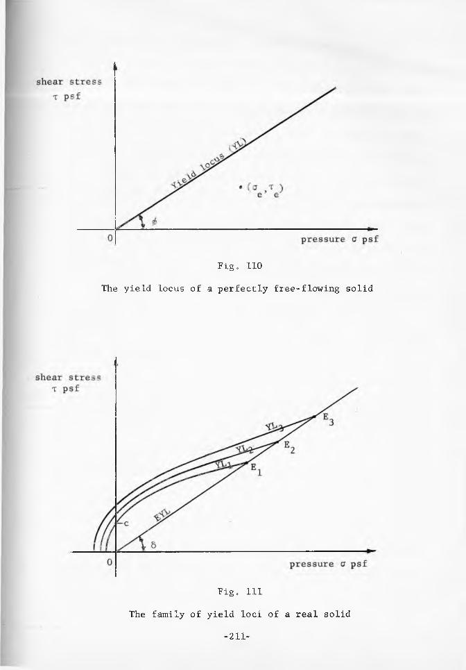
Fig. 110
The yield locus of a perfectly free-flowing solid
Fig. Ill
The family of yield loci of a real solid
-211-

Now obstructions to flow are considered. It is postulated that,
if the flowing solid develops enough strength to support its own weight
in some stable structure over or about the outlet of the channel, then
that structure will form and flow will not occur. The two typical
structures which form obstructions to flow are: a dome across the
channel, and a vertical (or almost vertical), circular, empty pipe
circumscribing the outlet. For flow to prevail, the stresses in these
structures must exceed the strength of the solid so that the structures
fail. Since failure usually originates in a thin layer at the surface
of an obstruction, the stresses which act at some point of the surface
and the yield strength which the solid develops at that point of the
surface are critical.
The stresses which act at the surface of a dome, (a,) , , and of1 domea pipe, (a,) . have been determined in the analysis of incipient r r 1 pipefailure. The yield strength which a solid develops at an exposed
(traction-free) surface is called the unconfined yield pressure, f ,
and is assumed to have been generated by the major consolidating pressure
of flow, hence
f = f (aj. (a)c c 1
In the calculations it is more convenient to operate with forces
(V.). = A(a ) (V ) . = A(a.) . ,1 dome 1 dome, 1 pipe 1 pipe
V, = A a.. and F = A f ,1 1 c cwhere A is the area of the cross-section of the shear cell used to
measure the flow properties (Part V ) . Relation (a) then transforms into
-212-

lb
Fig. 112
Flow-functions
The flow, no-flow condition
-213-
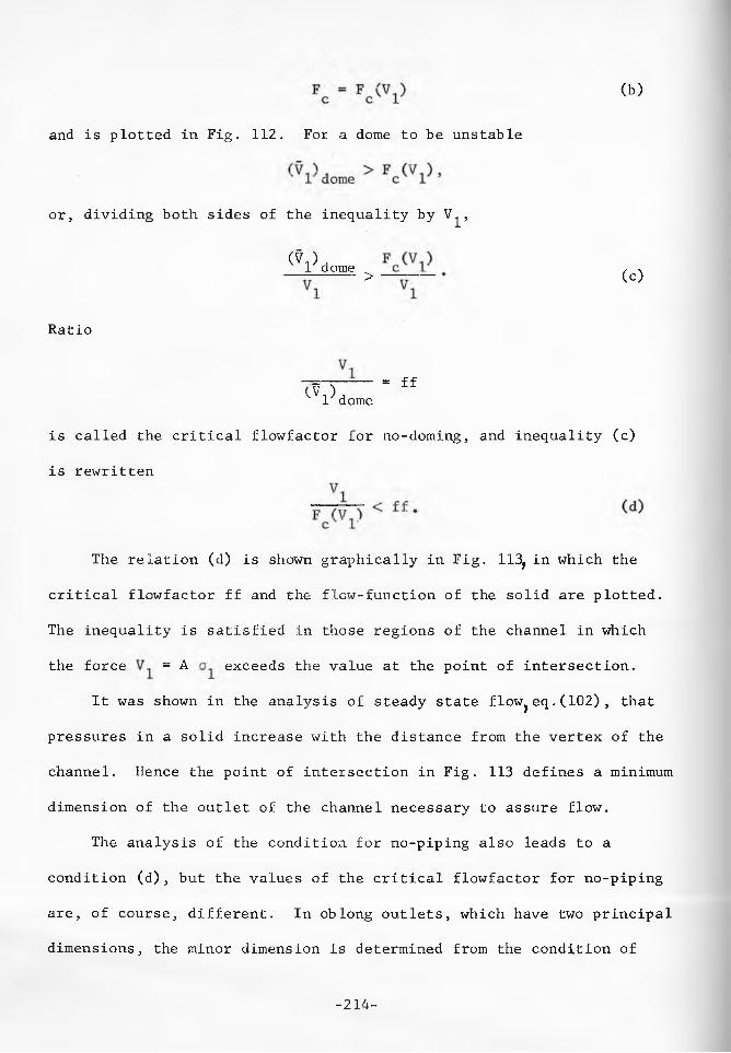
(b)
and is plotted in Fig. 112. For a dome to be unstable
or, dividing both sides of the inequality by V^,
l V d o Be > (c)
Ratio
o n ----- ff1 dome
is called the critical flowfactor for no-doming, and inequality (c)
is rewritten
The relation (d) is shown graphically in Fig. 113? in which the
critical flowfactor ff and the flow-function of the solid are plotted.
The inequality is satisfied in those regions of the channel in which
the force = A exceeds the value at the point of intersection.
It was shown in the analysis of steady state flow}eq.(102), that
pressures in a solid increase with the distance from the vertex of the
channel. Hence the point of intersection in Fig. 113 defines a minimum
dimension of the outlet of the channel necessary to assure flow.
The analysis of the condition for no-piping also leads to a
condition (d), but the values of the critical flowfactor for no-piping
are, of course, different. In oblong outlets, which have two principal
dimensions, the minor dimension is determined from the condition of
-214-

no;-doming and the major dimension from the condition of no-piping.
In view of the fact that a pipe circumscribes the outlet, the major
dimension of an outlet is its largest dimension, e.g., the diagonal
of a rectangle.
It is useful to introduce a rough guide to the flowability of
solids by classifying them in accordance with the value of the ratio
•V-jVF of the flow-function. Namely,
10 < V^/F - free-flowing,
4 < < 1 0 - easy-flowing,
1.6 < V /F < 4 - cohesive,1 c
V^/F^ < 1.6 - very cohesive and non-flowing.
When a solid is flowing, the yield locus of an element of the .
solid and the value of F which the locus defines are functions of thecmoisture content of the solid H, its temperature T, and the major
consolidating pressure = V^/A acting on the element. For given H
and T, the relation F^ = F (V^) , plotted in Fig. 112,is called the
instantaneous flow-function of the solid and, together with angle 5, ..
determines the flowability of the solid under conditions of continuous
flow.
If flow in a channel is stopped and the solid is left at rest for
an interval of time t, say hours or days, it is assumed that the pressures
within the solid remain essentially unchanged, the solid keeps consolidat
ing with time, and may gain strength. The relation F ^ = Fc(V^,t)
obtained under these conditions is referred to as the time flow-function.
-215-
In Fig. 112, the latter usually lies above the instantaneous flow-
function, indicating a gain in strength with the time interval of
consolidation at rest. This gain may be caused by any one or a
combination of the following factors:
1. Eascape of entrained air with corresonding increase of
density and strength of the solid.
^ 2. ^External vibrations due to operating machinery, railroads, -----
or wind which cause a rearrangement of particles and an
increase in the consolidation of the solid.
3. Evaporation of free water with concurrent precipitation of
dissolved salts which cement the particles.
4. Break-up or softening of particles or crystals under pressure,
causing an increase in cohesion.
5. Chemical changes in the surface of particles, e.g., fermentation.
Particle Size. As a general rule, solids which do not contain
particles smaller than, say, 0.01 inch are free-flowing. There are
exceptions to this rule. For instance, grain ferments under adverse
moisture and atmospheric conditions and can develop sufficient strength
to cease being free-flowing. Soybean meal contains oil which under
conditions of high moisture and temperature binds the particles into
a non-flowing mass. Flaky or stringy materials, like wood shavings,
mica, asbestos, interlock and also form obstructions to flow. Most
ores, however, come under the general rule.
The flowability of a solid containing a range of sieve sizes, which
includes both, fine and coarse particles, is invariably governed by the
flow properties of the fine fraction. This is explained by the fact
that during flow the shearing takes place across the fines. The coarse
particles are a passive agent in this process. However, the size of
the coarse particles will affect the tendency to interlock at the
outlet, and the impact of the heavy, coarse particles charged into
a container may cause compaction of the solid along the trajectory
of the falling stream. ...
Limitations of the analysis
In the discussion of the yield stresses, the solid has been assumed
at rest, that means, the influence of the velocities and accelerations
on the stresses has been neglected. To understand the implications of
these simplifications it is necessary to consider the effect of velocity and acceleration. An element of a solid flowing down a channel under
goes a change of pressure which changes the bulk volume of the element
and, hence, the volume of voids within the element. Unless the solid
is in a vacuum, changes in the volume of voids set up gas pressure
gradients in the mass. Since these gradients are not included in the
analysis, they must be negligible, hence, the velocities of flow must
be low.
In the analysis of the stress fields, the equations of equilibrium
have been used. For these equations to be applicable, the dynamic
forces must be negligible, compared to the gravitational forces, Hence,
the accelerations of the particles must also be low.
-217-

These restrictions on the velocity and acceleration are not too
serious. The analysis applies to most cases of flow controlled by
means of feeders. However, the work may not apply to cases of free
fall out of a hopper, and does not apply to free fall through any
channel of constant cross-section, like a straight spout. Some of
these problems are now under study. The present work does not give any
absolute values of velocities. Where velocities are mentioned, the
values are only relative to some asigned value; e.g., the velocity
profiles, Figures 68, 69 and 70, have a unit yelocity at the axis
of the channels and give the relative values at other points of a
cross-section of the channel.
For controlled flow, this work prescribes the dimensions, shapes,
and wall properties of channels necessary to assure a given type of
flow to a solid of given flow properties.
Types of flow
A solid may flow in a channel made of an extraneous material,
like steel, concrete, wood, or it may form a channel within itself.
In both cases, the boundaries between the flowing mass and the station
ary, confining material will be called walls. Walls made of an
extraneous material will be referred to as weak walls, and walls formed
within the solid itself will be referred to as rough walls. The
frictional and cohesive strength of a rough wall is usually the same as
that of the flowing solid and, hence, is described by the flow propert
ies of the solid (angle S and flow-function). A weak wall introduces
-218-
a degree of weakness, compared to a rough wall; the strength of a weak
wall depends on both, the flowing solid and the material of the wall,
and is measured by the angle of friction S' under conditions of sliding.
Mass flow is said to occur within a channel made of an extraneous
material when the solid flows everywhere along the weak walls of the
channel. For complete mass flow to occur, the walls must be sufficiently
steep and smooth (weak), and the channel must not have any sharp corners,
abrupt transitions, or discontinuities in the frictional properties of
the walls. Any one of the last three conditions will enforce a dead
region in its vicinity, though mass flow may prevail in the remainder
of the channel.
Mass flow is characterized by uniform and comparatively low
velocities, because the flow pattern is steady and flow takes place
across the whole section of the channel. This type of flow is partic
ularly advantageous when an even rate of draw is required or when the
solid is to provide a seal against gas counter-flow. Mass flow is well
suited to fine solids which have a tendency to flood upon aeration.
Mass flow can assure a first-in, first-out flow sequence which is vital
when the flowing solid is subject to deterioration with time, or when
the solid segregates while charged into the container. While this flow
pattern does not prevent segregation during charging it can cause
remixing during flow.
The containers which lead to mass flow have also disadvantages:
they are tall for a given capacity, they require extensive forming to
provide a smooth channel, the walls wear out as the solid continuously
-219-
slides on them. These things add to the expense. Mass flow containers
for coarse solids should not have steep walls, because large rocks
carry a great deal of momentum when charged into a container and when
they hit the mass deposited in a steep hopper they tend to wedge the
solid within the walls and cause it to dome across the channel.
Typical mass flow containers are shown in Figures 114. Containers
(a), (c) and (d) have no sharp corners and give perfect mass flow.i ...
The other containers will have dead regions as shown by dashed lines.
A dead region at a transition contains a core (area ABC in Fig. 25)
within which the solid is not flowing at all, and approaches, above
and below the core, in which flow is very slow. If the solid develops
strength with the time of consolidation at rest, the dead regions gain
strength and may provide substantial abutments which constrict the
channel and may lead to doming at the transition. This phenomenon is
frequently observed and can be corrected by filling in the sharp
corners to provide the effect of the smooth transition shown in Fig.
114 (c). The filling material should be the same as the material of
the walls, and the radius of curvature of the smooth transition
should be sufficiently large. The work on what constitutes a 'suff
iciently large' radius is now in progress. At this stage, it is
recommended that the radius of the transition be equal to one half
the width of the vertical portion of the channel.
The selection of the hopper slopes for mass flow is done on the
basis of the effective angle of friction of the solid 5, and the angle
of friction between the solid and the wall The values of these
-220- .

two angles are obtained from the tests described in Part V.
For conical, circular hoppers, Fig. 114 (a) and for conical
hoppers with a smooth transition, Fig, 114 (c) the selection is based
on the charts given in Figures 85 to 89. These charts have been computed
for axially symmetric radial flow and represent quite closely the
conditions which occur in conical hoppers. The abscissa in the charts
is 0', the slope of the hopper walls measured from the vertical;
the ordinate, which is of interest in this part of the work, is the
angle It will be noticed that the regions within which solutions
are available are bounded. If a wall described by same pair
is selected outside of such a region, flow along the wall will not
occur, though flow may occur across the solid in a vertical, or
almost vertical, pipe circumscribing the outlet. There is no in-
between stage, if flow occurs, it occurs either along the weak walls
or in a pipe. This means that, for a given angle of friction 6',
a maximum slope angle 0' is prescribed by the charts.
In measuring angle f ' , there is usually some scatter and a range
of values is obtained. For the purpose of design it is safe to use an
upper value of the range. The charts are plotted for five values of 5:
30°, 40°, 50°, 60°, 70°. Since the actual value of 5 will usually lie
in between two of these values, the maximum value of 0' is obtained by
interpolation between the values obtained from the appropriate charts.
For design, the interpolated value of 0 1 is reduced by 3° to 5°. It
can then be said with a high degree of certainty that mass flow will
occur in the channel for practically all levels of the solid in the
-221-

channe1.
Containers with conical hoppers have advantages: the shells are
light and require no lateral reinforcement, because they do not
transfer any bending stresses; their shape is regular, hence they are
easy to design and to fabricate; the hoppers can often be brought to
quite small outlets which require but small feeders or valves.
However, conical hoppers have a serious disadvantage in the comparatively
high headroom which they need for a given capacity. High headroom is
expensive since it requires a high structure, a high elevation of the
solid, often a high building.
The height of a container can frequently be reduced by providing
a hopper with an oblong outlet rather than a circular one. In such
a hopper, Figures 114 (e), (f), (g), the slope of the end walls is
either vertical or as described above for the circular hoppers, but
the slope of the side walls can be considerably less. A mathematical
determination of the flow criteria in hoppers of these shapes is not
feasible at this time. From observation, it appears, however, that
in the central part of an oblong cross-section flow closely approaches
a pattern of plane flow (referred to as plane strain in the previous
parts of this work). Plane flow is the type which would occur in
the container, Fig. 114 (g), if the dimension L were infinite and flow
were uniform along the whole length L. Plane flow has been analyzed
mathematically. In particular, plane radial flow, which is approached
in straight hoppers, has been analyzed and the selection charts are
presented in Figures 80 to 84 for symmetric channels, for 6 = 30°,L ) r
-222-

(f) (g)
Fig. 114 ,
Mass-flow containers
-223-
40°, 50°, 60°, and 70°. In addition., selection charts for asymmetric channels with one vertical weak wall and the. other wall sloping at an
angle 0 1 are given in Figures 90 to 92 for 6 = 50°, and for three
frictional values of the vertical walls = 20°, 30°, and 40°.
As is seen from these charts, the regions of Q' ,j>' for which
solutions are available in plane radial flow are much larger than the
corresponding regions in conical flow. This means that plane radial
flow can occur m.thin less steep and rougher walls. Indeed, in plane
flow, 0* = 90° - 0' at the bounds. However» these, very high values
of 0' are practically unattainable nor: only because plane radial flow
is never actually reached in channels of oblong cross-section but also
because plane radial flow is not approached from the top of the
channel until a sufficiently high pressure has been developed in the
solid. Consider a case of plane flow in a wedge-shaped channel, Fig. 115.
The magnitude of the major pressure a. which acts within the solid
along the wall of the channel is plotted in the figure with a continu
ous line. The pressure required for plane radial flow is given by
eq.(102), and is plotted with a dashed line. At some height h above
the outlet the two lines separate and this causes the flow channel to
break away from the walls and approach the vertical. The shaded
regions of the solid may remain stationary for some time and then
slide down like rigid bodies. Having gained strength during the con
solidation at r e s t , the shaded regions may cause an obstruction to flow
as they descend bodily toward the narrower section of the hopper.
Thus, to ensure plane mass flow, the channel should either be very
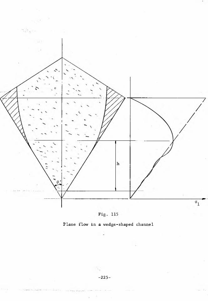
//1
Plane flow in a wedge-shaped channel
-225-
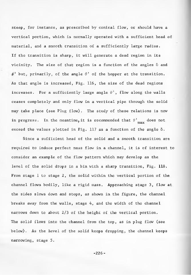
steep, for instance, as prescribed by conical flow, or should have a
vertical portion, which is normally operated with a sufficient head of
material, and a smooth transition of a sufficiently large radius.
If the transition is sharp, it will generate a dead region in its
vicinity. The size of that region is a function of the angles 6 and
but, primarily, of the angle 6' of the hopper at the transition.
As that angle is increased, Fig. 116, the size of the dead regions
increases. For a sufficiently large angle S', flow along the walls
ceases completely and only flow in a vertical pipe through the solid
may take place (see Plug flow). The study of these relations is now
in progress. In the meantime, it is recommended that 0' does not r & 7 maxexceed the values plotted in Fig. 117 as a function of the angle 5.
Since a sufficient head of the solid and a smooth transition are
required to induce perfect mass flow in a channel, it is of interest to
consider an example of the flow pattern which may develop as the
level of the solid drops in a bin with a sharp transition, Fig. 118.
From stage 1 to stage 2, the solid within the vertical portion of the
channel flows bodily, like a rigid mass. Approaching stage 3, flow at
the sides slows down and stops, as shown in the figure, the channel
breaks away from the walls, stage 4, and the width of the channel
narrows down to about 2/3 of the height of the vertical portion.
The solid flows into the channel from the top, as in plug flow (see
below). As the level of the solid keeps dropping, the channel keeps
narrowing, stage 5.
-226-
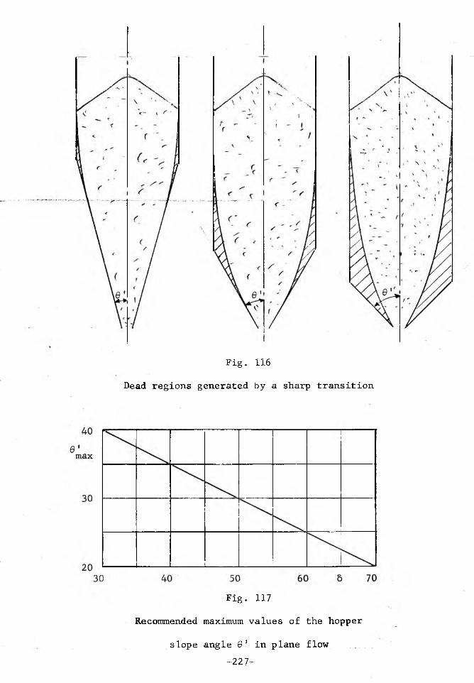
Fig. 116
Dead regions generated by a sharp transition
Fig. 117
Recommended maximum values of the hopper
slope angle 9 ' in plane flow.....-227-

It should be stressed that square and rectangular bins, shown in
Fig. 119 (a) and (b), do not produce mass flow. The sharp corners
fill out with packed solid and flow along the walls cannot occur.
Mass flow may be approached if the corners are sufficiently rounded
off, Fig. 119 (c), but no specific design recommendations can be made
at this time without experimentation.
Hoppers with one vertical wall. The influence of the asymmetry
of a hopper on the critical flowfactor has been analyzed for plane flow
for the angle 6 = 50°, and for three angles of friction <t? between
the solid and the vertical wall, Figures 90 to 92. A comparison of
these values of the flowfactors with those plotted in Fig. 82 for the
corresponding symmetrical channel shows that the minimum values are
not affected by asymmetry, but the trough of minimum values is shifted
by asymmetry toward the larger values 0',^'. For walls of a given
frictional value and a given critical flow-factor the allowable included
angle is, in general, greater in symmetry than in asymmetry. For
instance, for <b' = = 40°, ff = 1.3, in symmetry 20' = 40°, in
asymmetry 0' = 35°. A channel with one vertical wall may have an
advantage if mass flow fails to develop, because a break along a
rough wall (01 =0) occurs at lower values of the flowfactor in the
asymmetric channel. For instance, for 0' = 0, $ = 40°, fa ' « 6 =50°
(rough vertical wall), ff = 1.8 in symmetry, but only 1.36 in asymmetry.
Further, a symmetric hopper with a vertical partition, Fig. 120, permits
a somewhat larger included angle than a similar hopper without the
partition. However, it should be observed that to obtain a controlled
-228-

Fig. 118
Usual sequence in plane flow
-229-

effect the partition must be sufficiently strong to stand up to the
difference between the pressures on each side. Should one side dome
and the other empty out, the resultant pressure may be substantial.
Plug flew occurs when a channel either has no weak walls (storage
pile, flat bottom bin) or the walls are not sufficiently steep and
smooth for mass flow to develop. The solid then forms a channel
within itself and flows within rough walls.
Conical flow within rough walls narrows down to values of 0 1 which
are at most as given in Table 2, page 68. More often, 0' is zero and
the channel is vertical: flow takes place in a vertical pipe. The
diameter of such a channel approaches the largest dimension D of the
outlet, That dimension is the diameter of a circular outlet, the
diagonal of a square or rectangular outlet, etc. The transition from
the shape of the outlet to the circular pipe occurs within a height of
one to two diameters of the pipe. The transition is explained by the
fact that, at the sides of an oblong outlet or of a square, outlet, the
condition of plane radial flow is approached and, hence, the angle 0'
Fig. 121, is larger at the sides than at the ends or corners of the
outlet where conical flow is approached.
As the solid flows along a rough wall, a degree of weakness
develops along it. It is not practical to try to measure that weak
ness, nor does the effort seem to be justified. It is sufficient to
estimate the value of the angle <£>' by taking an average value# between
# That value of & ' is probably approached from an original corresponding to \|r1 - 90° = 45°, at which flow starts without a velocity discontinuity along the wall. As flew continues, a weakness develops.If ratio °f the solid permits, flow may start along a slip line
-230-

& and the value of </>' corresponding to i|rr ~ 90° = 45° „ E. g„ for = 50°,
Fig. 82°, 4>' = %(50 + 38) = 44°. •
Calculation of the dimensions of the outlet
The dimensions of the outlet of a channel should be sufficient to
prevent: (a) doming, (b) piping, (c) particle interlocking, and to
provide the required rate of draw.
(a) Doming. The critical value of the flowfactor ff is read from
the appropriate chart, Figures 80 to 92, for the selected wall conditions
(0 1 , 6'). In order that a solid does not dome at the outlet, the ratio
V../F at the outlet must exceed the value of the critical flowfactor ff.1 cThe flowfactor is plotted together with the appropriate flow-function
and the critical value of F^ is read at the point of irt ersection,
Fig. 113. For circular outlets the diameter is then computed from the
relation
B > 2Fc/A r, (158)
for square outlets, the side of the square is found from
• B ^ 1.8 Fc/A r, (159)
and for oblong outlets of ratio length to width in excess of 2.5 the
width is found from
B >>. Fc/A y. " (160)
The flow-function to be used in this analysis depends on the
operation. For continuous operation, the instantaneous flow-function
should be used; for intermittent operation, the time flow-function
measured for the time interval of the stoppages should be used.'with a velocity discontinuity occurring from the beginning.
-231-
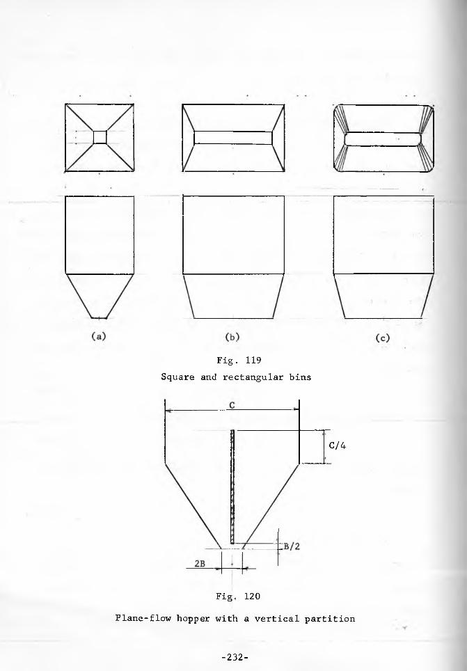
Fig. 119 Square and rectangular bins
C/4
Fig. 120
Plane-flow hopper with a vertical partition
-232-
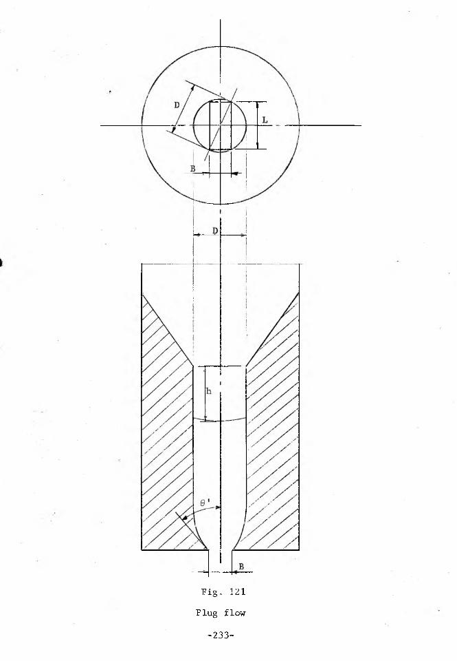
Fig. 121
Plug flow
-233-

The latter will sometimes call for an impractieally large dimension.
If, concurrently, the instantaneous flow-function gives a reasonable
dimension, then the latter should be selected and a flow promoting
device should be applied. Flow promoting devices are very effective
in starting the flow of solids which pack when at rest but flow well
under continuous operation.
For many solids, this analysis does not produce any minimum
dimension of B, because the flow-function curve lies completely below
the critical flowfactor line. On the other hand, the flow-function
curve may be completely above the critical flowfactor line; this would
indicate that the solid will not flow by gravity.
(b) Piping. This analysis applies to channels in which plug
flow is expected. In plug flow, Fig. 121, as the solid is drawn out
of the bin and the channel empties out, some height h of the vertical
pipe may become exposed before a layer of the solid outside the pipe
fails and slides into the channel. The height h at which the pipe
fails depends on the diameter of the channel. For a given value of
strength of the solid, the channel becomes less stable with an increase
in diameter D. The channel is least stable when the diameter is
infinite, which occurs in plane flow. The height of an exposed pipe
should not be excessive because the failure and the drop of a deep
layer of the solid creates considerable impact and may pack the solid
within the pipe and cause doming. On the other hand, if the solid
contains fines and is prone to aeration, such a drop may cause a
flooding of the feeder. A large value of h may also lead to a significant

reduction in the live storage capacity. In an extreme case the empty
pipe may extend through the full height of the bin, silo or pile.
Since the pipe circumscribes the outlet, the largest dimension
of the outlet determines the diameter of the pipe. The largest dimen
sion D is the diagonal of a square or rectangular outlet, or the diameter
of a circular outlet. While the solid flows within the pipe, the
solid outside the pipe is at rest and undergoes consolidation with
time. Hence, the effect of time is of considerable importance in this..
analysis, and the time flow-function should be used in this part of the
analysis.
Contours of critical flowfactor values are plotted in Fig. 96 as
a function of the effective angle of friction 5 and the angle of
internal friction obtained from the time yield locus in the manner
shown in Fig. 95. The applicable value of the flowfactor ff is now
superposed over the appropriate time flow-function, Fig. 113, and the
critical value of is obtained at the point of intersection of the
two lines. The required dimension D is found from the formula
v < 1 6 1 >Ay dn nB l
The factor 4(dco/dn)n_^ is plotted as a function of $ in Fig. 122, line a.
For solids which are not affected by consolidation at rest, i.e.
for solids whose time flow-function differs little (say, by less than
10%) from the instantaneous flow-function, a simpler analysis is
offered. The value of the flowfactor is read off Fig. 97 for the
appropriate value of the angle 5. Then the critical value of F^ is
-235-

obtained, as above, and the dimension D is found from eq. (161) with
the factor 4(dco/dn)n_^ taken from Fig. 122, line b for the given value
of the angle 5. It will be noticed that in these solids piping is
unlikely to occur for 5 < 54.5°.
If the flow-function lies completely below the critical flowfactor,
the solid will not pipe; on the other hand, if the flow-function lies
completely above the critical flowfactor, or the point of inter
section indicates an impractically large dimension D, piping will
occur about the outlet unless the container is designed for mass flow.
(c) Particle interlocking. Solids which do not contain fines
are usually free flowing and the size of the outlet needs to be only
large enough to assure the required rate of flow without interlocking
of the particles. It is not possible to specify outlet dimensions
which will apply to all solids under all circumstances. The guide
shown in Fig. 123 applies to particles of uniform shape, but not to
chips, flakes and fibres. d is the intermediate dimension of the
largest particles; the area A and the dimension B of the outlet
should exceed the plotted values.
Influence of dynamic over-pressures
So far, the developed flow criteria have neglected all pressures
due the acceleration or deceleration of the flowing particles. It is
of course inherent in the theory of plasticity, which is the basis for
this work, to neglect the velocity terms and to apply the equations of
equilibrium instead of the equation of momentum in the development of
-236-
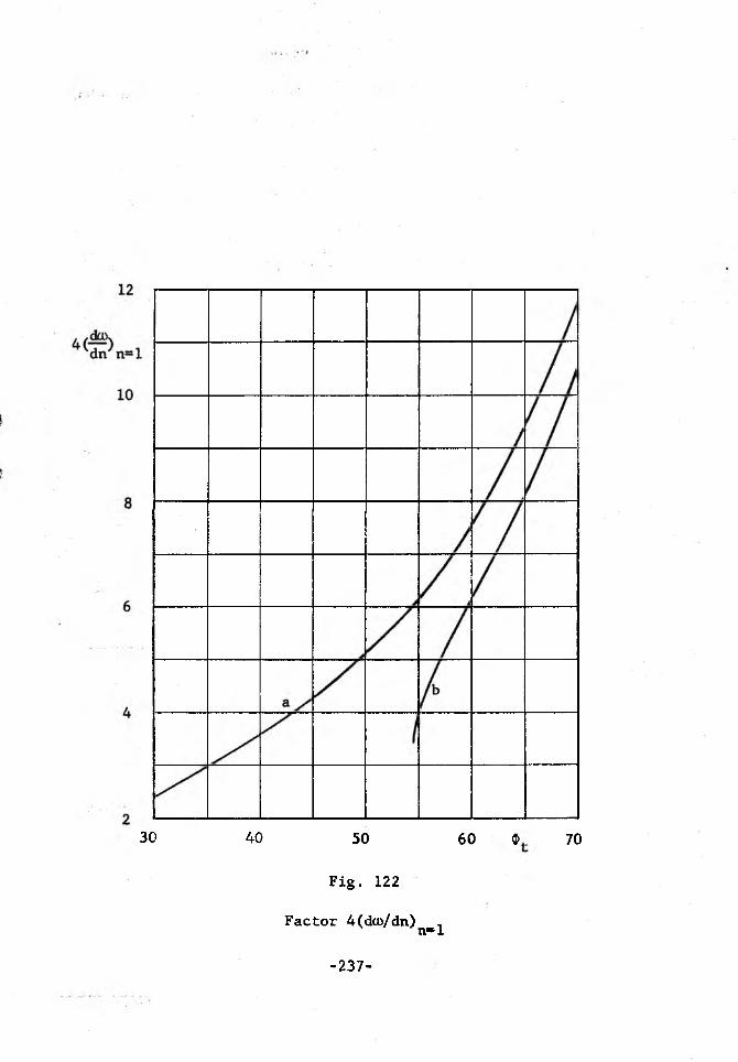
30 40 50 60 # 70
Fig. 122
Factor 4(dco/dn) ..n® I
-237-

of the stress field. This implies that the velocities throughout the
mass are low so that the accelerations which exist in steady state flow
be negligible. Steady state flow is an ideal which is approached
by a suitably design of the channel and of the feeder but which is
Non-steady flow is also prevalent in vertical channels. Hence,
it is prevalent under most conditions of plug flow. Another condition
leading to non-steady mass flow can be inferred from the plots of the
conical fields. These fields extend only within well defined regions
in the coordinates. Outside of these regions steady state flow
cannot occur. If the slope of the wall 0' and the frictional conditions
at the wall are such that point (0',^') lies close to the bound of
the field, then it can be expected that a slight momentary change in
<i>' may move the point over the bound, thus momentarily stopping flow.
Many solids exhibit a slip-stiek effect: their angles of friction vary
over wide limits. These solids have a strong tendency for non-steady
pulsating flow.
The accelerations and decelerations superimpose dynamic pressures
over the consolidating pressures of steady state flow, causing an
additional consolidation of the solid and developing additional strength
in it. These dynamic pressures become more pronounced as the velocities
of the particles increase. For a given rate of flow of a solid through
a channel, the velocities increase with the reduction of the cross
sectional area of the channel. Hence, as the area decreases toward
For one thing, flow has to be started
and stopped, and that involves acceleration and deceleration.
-238-

Fig. 123
Dimensions of outlets to avoid particle interlocking
-239-
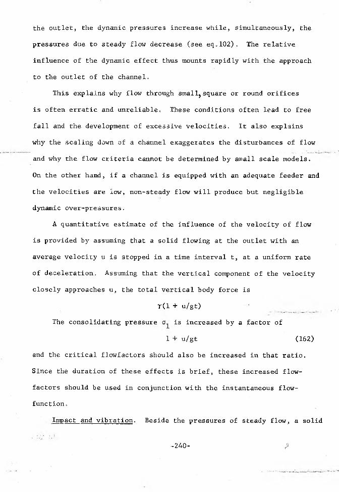
the outlet, the dynamic pressures increase while, simultaneously, the
pressures due to steady flow decrease (see eq„102). The relative
influence of the dynamic effect thus mounts rapidly with the approach
to the outlet of the channel.
This explains why flow through smalljsquare or round orifices
is often erratic and unreliable. These conditions often lead to free
fall and the development of excessive velocities. It also explains
why the scaling down of a channel exaggerates the disturbances of flow
and why the flow criteria cannot be determined by small scale models.
On the other hand, if a channel is equipped with an adequate feeder and
the velocities are low, non-steady flow will produce but negligible
dynamic over-pressures.
A quantitative estimate of the influence of the velocity of flow
is provided by assuming that a solid flowing at the outlet with an
average velocity u is stopped in a time interval t, at a uniform rate
of deceleration. Assuming that the vertical component of the velocity
closely approaches u, the total vertical body force is
T( 1 + u/gt) -
The consolidating pressure is increased by a factor of
1 + u/gt (162)
and the critical flowfactors should also be increased in that ratio.
Since the duration of these effects is brief, these increased flow
factors should be used in conjunction with the instantaneous flow-
function.
Impact and vibration. Beside the pressures of steady flow, a solid
-240- ?
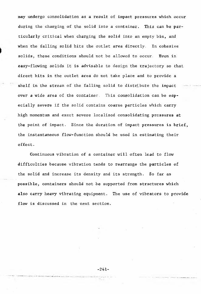
may undergo consolidation as a result of impact pressures which occur
during the charging of the solid into a container. This can be par
ticularly critical when charging the solid into an empty bin, and
when the falling solid hits the outlet area directly. In cohesive
solids, these conditions should not be allowed to occur. Even in
easy-flowing solids it is advisable to design the trajectory so that
direct hits in the outlet area do not take place and to provide a
shelf in the stream of the falling solid to distribute the impact
over a wide area of the container. This consolidation can be esp
ecially severe if the solid contains coarse particles which carry
high momentum and exert severe localized consolidating pressures at
the point of impact. Since the duration of impact pressures is brief,
the instantaneous flow-function should be used in estimating their
effect.
Continuous vibration of a container will often lead to flow
difficulties because vibration tends to rearrange the particles of
the solid and increase its density and its strength. So far as
possible, containers should not be supported from structures which
also carry heavy vibrating equipment. The use of vibrators to provide
flow is discussed in the next section.
-241-

Flow promoting devices
Since this work is on the subject of gravity flow of solids,
devices such as extruders, used to cause the flow of solids which are
inherently unsuited for gravity flow, will not be discussed. A
solid is not suitable for gravity flow if its instantaneous flow-
function lies above the minimum critical flowfactor applicable to
the solid. For instance, a solid of 6 = 50° has a minimum flow
factor of about 1.035 in plane flow for <b' = 20°, Fig. 82. If the
ratio V,/F of the instantaneous flow-function of the solid is less 1 cthan this value for the practical range of pressure a = V^/A, then
the given solid is not suitable for gravity flow. If the instantaneous
flow-function lies below the minimum critical flowfactor then the solid
is suitable for gravity flow even though its time flow-function may
lie above the flowfactor. In the latter case, the application of a
flow promoting device is in order.
It is not proposed to discuss the respective merits of all the
available devices but to describe those combinations of hoppers and
flow promoting devices which seem particularly well suited to handle
certain classes of solids. Mass flow and plug flow will be considered
separately.
In a mass-flow bin, the solid slides along the walls and the
introduction into the hopper of any device, like an air pad, pulsating
panel, planetary arch breaker, would destroy the flow pattern and is
not acceptable. Flow in such a bin can be effectively promoted by the
application of either a vibrator or an air (or other gas) pressure
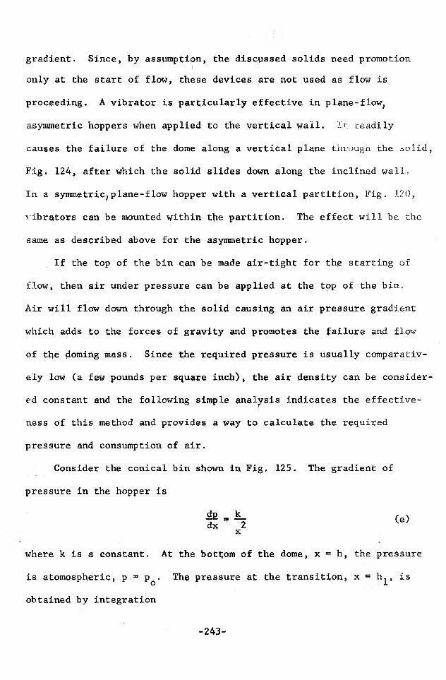
gradient. Since, by assumptipn, the discussed solids need promotion
only at the start of flow, these devices are not used as flow is
proceeding. A vibrator is particularly effective in plane-flow,
asymmetric hoppers when applied to the vertical wall. It readily
causes the failure of the dome along a vertical plane through the solid,
Fig. 124, after which the solid slides down along the inclined wall.
In a symmetric,plane-flow hopper with a vertical partition, Fig. 120,
vibrators can be mounted within tfie partition. The effect will be the
same a^ described above for the asymmetric hopper.
If the top of the bin can be made air-tight for the starting of
flow, then air under pressure can be applied at the top of the bin.
Air will flow down through the solid causing an air pressure gradient
which adds to the forces of gravity and promotes the failure and flow
of the doming mass. Since the required pressure is usually comparativ
ely low (a few pounds per squ$i?e inch), the £ir density can be consider
ed constant and the following simple analysis indicates the effective
ness of this method and provides a way to calculate the required
pressure and consumption of air.
Consider the conical bin shown in Fig, 125. The gradient of
pressure in the hopper is
t ’ h <*>X
where k is a constant. At the bottom of the dome, x « h, the pressure
is atomospheric, p = p q . The pressure at the transition, x h^, is
obtained by integration
-243-
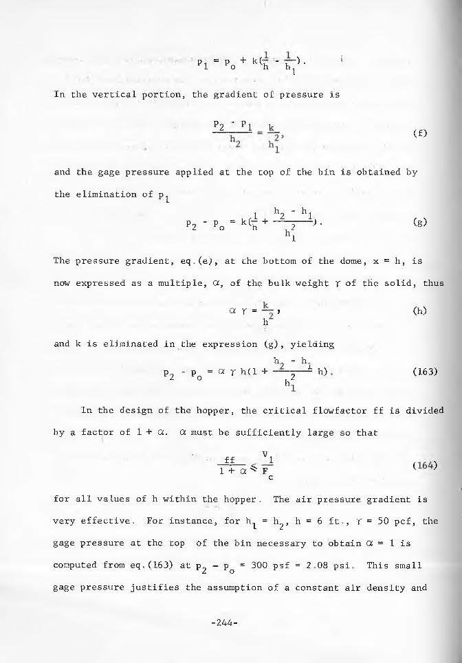
P1 ’ po + k(h - h^- S
In the vertical portion, the gradient, of pressure is
p2 ' P1 k_ (f)
and the gage pressure applied at the top of the bin is obtained by
the elimination of p^
1 ^2 ” ^1P 2 ' p o ' k(h + ~2--- > ■ (g)
hl
The pressure gradient, eq.(e), at the bottom of the dome, x = h, is
now expressed as a multiple, OC, of the bulk weight T of the solid, thus
a T = > (h). h .
and k is eliminated in the expression (g), yieldingh - h
p2 " Po = “ T h(1 + ~ 2 ~ ^ h) • (163)hi
In the design of the hopper, the critical flowfactor ff is divided
by a factor of 1 + Oi. (X must be sufficiently large so that
- Vff „ 1 -1+ a ^ f ^c
for all values of h within the hopper, The air pressure gradient is
very effective. For instance, for h. = h^, h = 6 ft., r = 50 pcf, the
gage pressure at the top of the bin necessary to obtain (X = 1 is
computed from eq.(163) at P2 ~ PQ = 300 psf = 2.08 psi„ This small
gage pressure justifies the assumption of a constant air density and
-244-

Vibrator at a vertical wall of a plane flow hopper
' Fig. 125
Air pressure gradient applied to promote flow
-245-
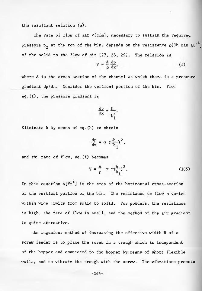
the resultant relation (e).
The rate of flow of air V[cfm], necessary to sustain the required
pressure p^ at the top of the bin, depends on the resistance p[lb min ft” ]
of the solid to the flow of air [27, 28, 29]. The relation is
where A is the cross-section of the channel at which there is a pressure
gradient dp/dx. Consider the vertical portion of the bin. From
eq.(f), the pressure gradient is
dp k dx “ r
\
Eliminate k by means of eq.(h) to obtain
i2 = a r(h-)2 dx U r('hi; 5
and the rate of flow, eq.(i) becomes
V = - a T(r“)2. (165)P
2In this equation A[ft ] is the area of the horizontal cross-section
of the vertical portion of the bin. The resistance to flow p varies
within wide limits from solid to solid. For powders, the resistance
is high, the rate of flow is small, and the method of the air gradient
is quite attractive.
An ingenious method of increasing the effective width B of a
screw feeder is to place the screw in a trough which is independent
of the hopper and connected to the hopper by means of short flexible
walls, and to vibrate the trough with the screw. The vibrations promote
-246-
the flow of the solid at the outlet without consolidating the solid
in the bin.
In plug-flow bins, any means that will break up a doming or piping
solid and start flow are acceptable [30]„ The usual methods are:
air pads, air jets, pulsating panels, knockers, vibrators, arch
breakers in the shape of stars, paddles, or planetary arms. In
view of the irregularity of plug flow, the selection and application
of these devices is likely to remain an art. Vibrators are effective
in these bins when used for final clearance. They are also effective in
starting flow, if installed in a vertical partition, but they should
only be used briefly, especially, if the instantaneous flow-function of
the solid is close to the critical flowfactor; otherwise, vibration
will tend to pack the solid.
-247-
Examples of design for flow
1. A fine solid whose flow properties are given in Fig. 126 is
to be stored in a quantity of 100,000 lb. The instantaneous flow-
function curve, F£(V^), lies below a flowfactor of 2.5; the time curve,
F^CVpt), lies higher. A mass flow bin with a conical hopper is
selected. From both, Figures 86 and 87, 0' = 20° for = 25°.maxSelect 0' = 15°, then the flowfactors at point 0' = 15°, £' = 25°
are respectively, 1.26 and 1.13 for 5 = 40° and 50°. For 5 = 48°^
interpolation gives ff = 1.16. In eq,(158) A = 1/13 sq ft and the
diameter of the outlet B > 2 x 1.25 x 13/19.2 = 1.7 ft.
The point of intersection of the flow-function with the critical
flowfactor lies at some distance from the lower test point of the flow-
function, hence, there is some uncertainty about the shape of the curve
at the point of intersection and about the exact value of F . It is,
therefore, advisable to increase the opening to, say, B = 2.0 ft.
The selected bin is shown in Fig. 127.
2. Another fine solid with flow properties given in Fig. 128
is to be stored in a quantity of 1Q0,000 lb. Here 5 ~ 40°. The time
flow-function is a straight line and coincides with a critical flow
factor of 1.4. A mass flow bin with a conical hopper is selected.
For 5 = 40°, Fig. 86 applies. Since 4>' = 19°, the solid will flow within
a range of hopper slopes 0' from 8° to 28°. For 0' = 0, ff = 1.65,
hence, the solid is likely to dome across a vertical channel. The bin
should have either no vertical portion, or only a short vertical portion,
as shown in Fig. 129, otherwise doming will occur from the transition up.
-248-
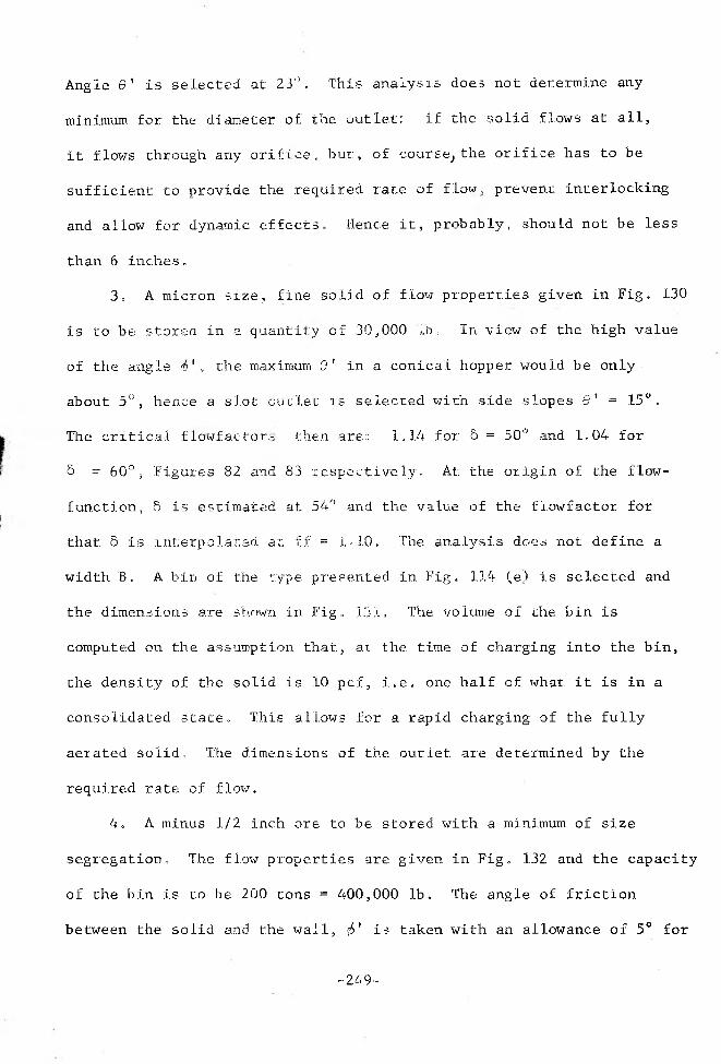
Angle 0' is selected at 23°. This analysis does not determine any
minimum, for the diameter of the outlet: if the solid flows at all,
it flows through any orifice, but, of course, the orifice has to be
sufficient to provide the required rate of flow, prevent interlocking
and allow for dynamic effects. Hence it, probably, should not be less
than 6 inches.
3. A micron size, fine solid of flow properties given in Fig. 130
is to be stored in a quantity of 30,000 A . In view of the high value
of the angle $1, the maximum 9 ' in a conical hopper would be only •
about 5°, hence a slot outlet is selected with side slopes 8' = 15°.
The critical flowfactor,- then are: 1,14 for 5 = 50° and 1.04 for
5 = 60°, Figures 82 and 83 respectively. At. the origin of the flow-
function, 5 is estimated at 54° and the value of the flowfactor for
that 5 is interpolated at. ff = .1. .10. The analysis does not define a
width B . A bin of the type presented in Fig, 1X4 (e) is selected and
the dimensions are shown in Fig, 13'.'.. The volume of the bin is
computed on the assumption that, at: the time of charging into the bin,
the density of the solid is 10 pcf, i.e. one half of what, it is in a
consolidated state. This allows for a rapid charging of the fully
aerated solid. The. dimensions of the outlet are determined by the
required rate of flow.
4. A minus 1/2 inch ore to be stored with a minimum of size
segregation. The flow properties are given in Fig, 132 and the capacity
of the bin is to be 200 tons = 400,000 lb. The angle of friction
between the solid and the wall, {4' i; taken with an allowance of 5° for
-24.9-
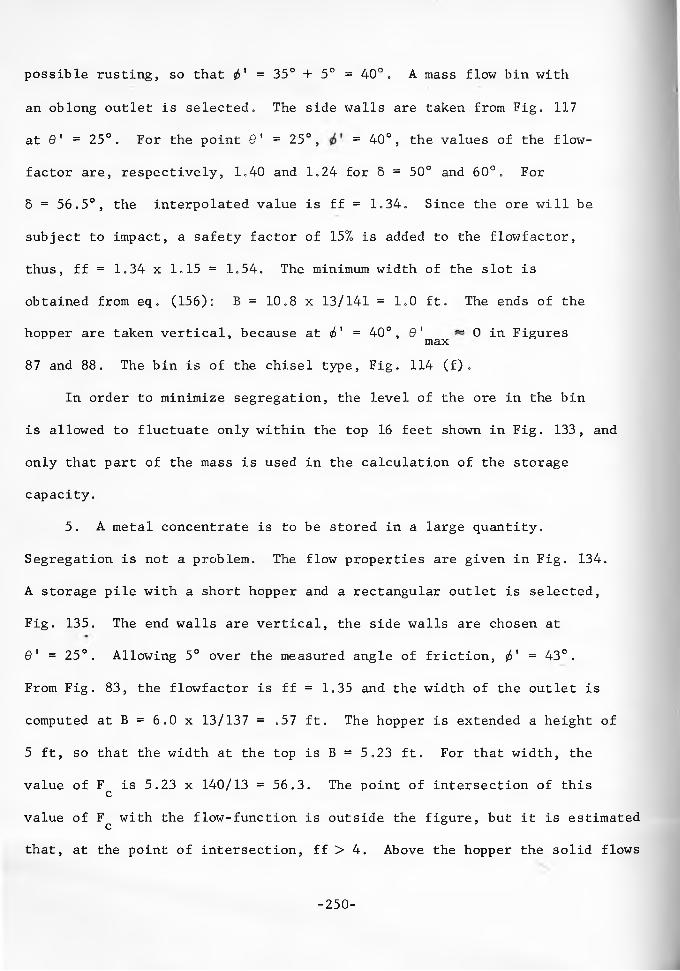
possible rusting, so that <t>' = 35° + 5° = 40°. A mass flow bin with
an oblong outlet is selected. The side walls are taken from Fig. 117
at 01 = 25°. For the point 0' = 25°, = 40°, the values of the flow
factor are, respectively, 1.40 and 1.24 for 5 = 50° and 60°. For
5 = 56.5°, the interpolated value is ff = 1.34. Since the ore will be
subject to impact, a safety factor of 157, is added to the flowfactor,
thus, ff = 1.34 x 1.15 = 1.54. The minimum width of the slot is
obtained from eq. (156): B = 10.8 x 13/141 = 1.0 ft. The ends of the
hopper are taken vertical, because at i 1 = 40°, 0' ~ 0 in Figuresmax87 and 88. The bin is of the chisel type, Fig. 114 (f).
In order to minimize segregation, the level of the ore in the bin
is allowed to fluctuate only within the top 16 feet shown in Fig. 133, and
only that part of the mass is used in the calculation of the storage
capacity.
5. A metal concentrate is to be stored in a large quantity.
Segregation is not a problem. The flow properties are given in Fig. 134.
A storage pile with a short hopper and a rectangular outlet is selected,
Fig. 135. The end walls are vertical, the side walls are chosen at
0' = 25°. Allowing 5° over the measured angle of friction, <f>' = 43°.
From Fig. 83, the flowfactor is ff = 1.35 and the width of the outlet is
computed at B = 6.0 x 13/137 = .57 ft. The hopper is extended a height of
5 ft, so that the width at the top is B = 5.23 ft. For that width, the
value of F is 5.23 x 140/13 = 56.3. The point of intersection of this cvalue of F^ with the flow-function is outside the figure, but it is estimated
that, at the point of intersection, ff > 4. Above the hopper the solid flows
-250-
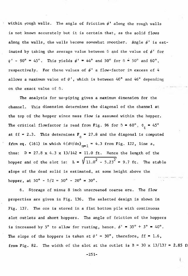
within rough walls. The angle of friction j>1 along the rough walls
is not known accurately but it is certain that, as the solid flows
along the walls, the walls become somewhat smoother. Angle is est
imated by taking the. average value between & and the value of <t>1 for
i|r1 - 90° = 45°. This yields - 44° and 50° for 5 = 50° and 60°,
respectively. For these values of <i>1 a flow-factor in excess of 4
allows a maximum value of 6 1, which is between 40° and 46° depending
on the exact value of 5. !
The analysis for no-piping gives a maximum dimension for the
channel. This dimension determines the diagonal of the channel at
the top of the hopper since mass flow is assumed within the hopper.
The critical flowfactor is read from Fig. 96 for 6 = 60°, <5 = 45°
at ff * 2.3. This determines F^ = 27.8 and the diagonal is computed
fr'om eq. (161) in which 4(d^/dn)n_^ = 4.3 from Fig, 122, line a,
thus: D = 27.8 x 4.3 x 13/142 = 11.0 ft. Hence the length of the
hopper and of the slot is: L = \ f 11.02 - 5.23^' = 9.7 ft. The stable
slope of the dead solid is estimated, at some height above the
hopper, at 50° - 5/2 = 50° - 20° = 30°. •
6. Storage of minus 8 inch unscreened coarse ore. The flow
properties are given in Fig. 136. The selected design is shown in
Fig. 137. The ore is stored in a flat bottom pile with continuous
slot outlets and short hoppers. The angle of friction of the hoppers
is increased by 5° to allow for rusting, hence, i>' = 35° + 5° * 40°.
The slope of the hoppers is taken at 6' = 30°, therefore, ff = 1.6,
from Fig. 82. The width of the slot at the outlet is B = 30 x 13/137 *= 2.85 ft
(-251-

30
T pcf
20
10
F lb c
V =■
; 19.2E»
s =
000
/
sa
t
T » C
Fc=1.2 5■n £ .
*• = 25°
70
60
550
40
30
0 1 2 3 4 5 6 7 8 9 10
Fig. 126
Example 1, Flow properties
-252-
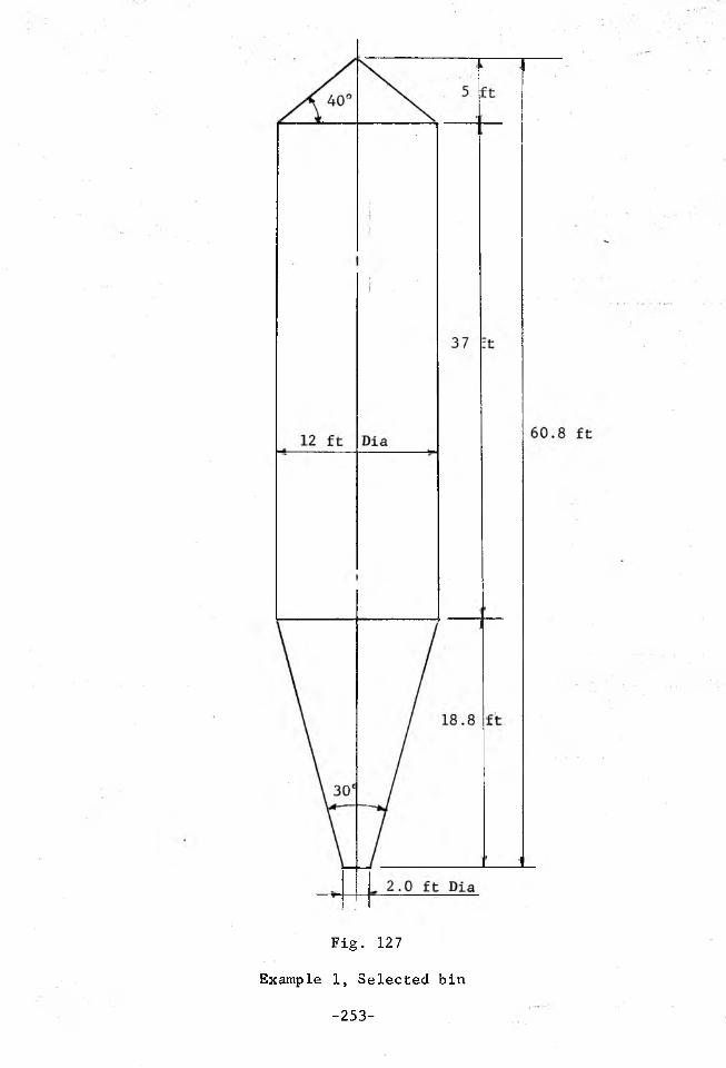
Fig. 127
Example 1, Selected bin
-253-

V 1 lb
Fig. 128
Example 2, Flow properties
-254-

Fig. 129
Example 2, Selected bin
-255”

0 1 2 3 4 5 6 7 8 9; 10
Fig. 130
Example 3, Flow properties

Example 3, Selected bin
-257-
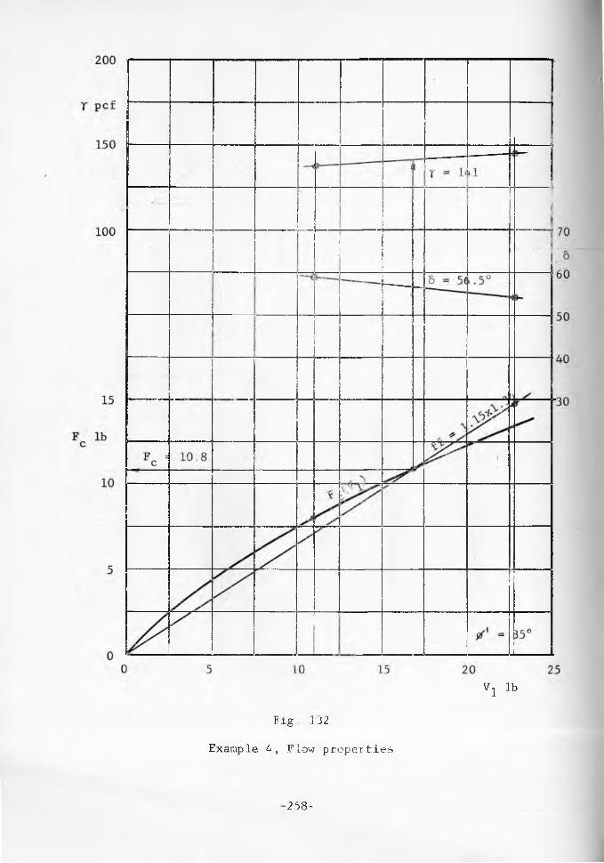
Fig 132
Example 4, Flow properties
V 1 lb
258-
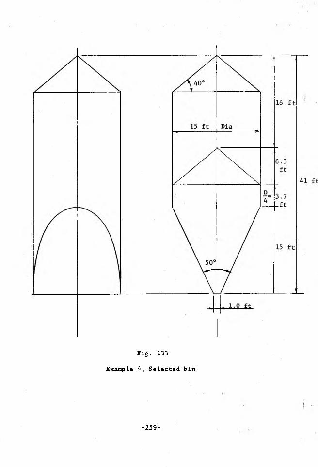
Fig. 133
Example 4, Selected bin
-259-
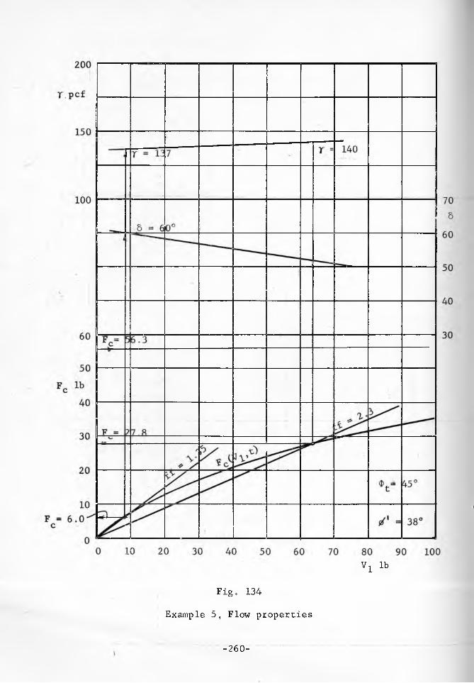
v l lb
F i g „ 134
Example 5, Flow properties
-260-

Fig. 135
Example 5, Selected hopper
-261-
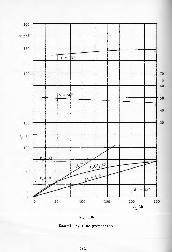
V 1 lb
F i g „ 136
Example 6, Flow properties
-262-

Fig. 137
Example 6, Selected hopper
-263-
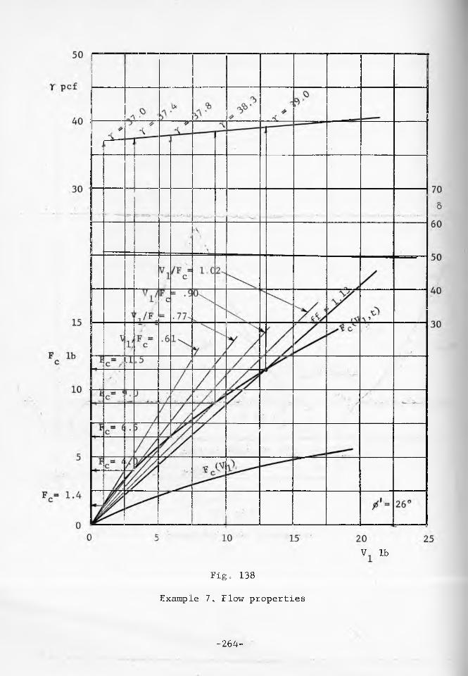
V lb
Fig „ 138
Example 7, Flow properties
-264-
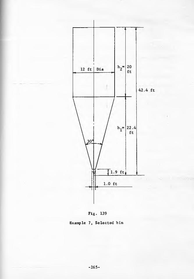
Fig. 139
Example 7, Selected bin
-265-

F c 1.4 4 .0 6.5 9.0 11.5
V ./ F 1 c .61 .77 .90 1.02 1.13
1 + a 1.85 1.47 1,25 1.11 1.00
a .85 .47 .25 .11 .00
r 37.0 37 .4 37.8 38.3 39.0
B .98 2.78 4.47 6.11 7.67
h 1.83 5.19 8 .34 11.40 14.30
1 - . 0048h .991 .975 .960 .945
N> 1 Xi o .40 .62 .53 .31 ■■ , —_ —
.00-------
Fig. 140
Example 7, Calculation of air pressure at top of bin
-266-
Above the hopper the ore flows on itself, i.e. within rough walls.
At the rough walls the angle </>' is again computed by taking the average
value between 5 = 50° and the value of <t>' corresponding to 1 - 90° - 45°.
This yields = 44°. The hopper walls are extended upwards until a
width B is reached at which ff = 3.5. This permits a maximum value
of 6 ' ss 46° at the base of the rough walls. That width is B = 71 x
x 13/148 = 6.23 ft. Above the base, the stable slope of the pile is
likely to be about 50° - S/2, or assuming 5 = 44° in that region,
50 - 22 = 28°. With the exception of the angle within the hopper,
no safety allowance has been made in these calculations, because the
use of the long, continuous slot makes it unlikely that a complete
obstruction will occur.
7. A feed product has flow properties shown in Fig. 138. For
8 = 50°, = 26°, the minimum critical flowfactor is ff = 1.13 in
conical flow. The time flow-function lies above that flowfactor up
to a value Fc = 11.5. Thus, the minimum hopper outlet for unassisted
flow is B = 2 x 11.5 x 13/39 = 7.67 ft. A bin with a conical hopper,
6' = 15°, and an outlet B = 1.0 ft, shown in Fig. 139, is selected.
Since the instantaneous flow-function lies well below the flowfactor,
Fig. 138, the one-foot outlet is ample, once flow has started. To
start flow, air pressure will be applied at the top of the bin. The
values of V,/F are read off Fig. 138 for four values of F . In the I c ctable of Fig. 140, the values of OC are computed from eq. (164) for ?
these four points; B is then computed at these points, and then
h = B/2 tan 0'. Then, in accordance with eq. (163), ~ PQ = Q!Yh(l-0.0048h
/144 psi. The gage pressure is plotted in the figure and shows a maximum
-267-
of 0.62 psi in the vicinity of h = 5.19 ft.
The resistance to the flow of air of this solid, p = 1.2 lb min ft
The rate of flow is found from eq. (165) for h = 5.19 ft, thus
V = A a r(h/h }2/p = it x 36 x .47 x 37.4(5.19/22.4)2/1.2 = 89 cfm.
Feeders
In this section it is not proposed to discuss the merits of the.....
various designs of feeders but to point out those features of design
which particularly affect flow, to describe the loads acting on the . .
feeders, and to report on two feeders which seem especially well
suited for certain materials and applications but have not received
the attention of industry which they deserve.
In a previous section, the method of calculating the dimensions
B and D of an outlet was described. It is now necessary to select
a feeder which will draw the solid through the whole specified cross
section B x D of the outlet. It will be realized chat many feeders act
ivate only a part of the area of the outlet, while the rest of the
outlet remains inactive (dead). Such is the case, Fig. 141, with
screw feeders of constant diameter and pitch, which draw only at the
back end of the outlet; with belt feeders, which can draw either at
the back or at the front, depending on the friction between the solid
and the belt, and switch from front to back as the friction changes
with changes of the moisture content in the solid; with rotary table
feeders, which tend to draw the solid only over the plow.
-268-
A feeder will draw along a length L, or a circumference itD in a
rotary table feeder, provided the capacity of the feeder increases
at a sufficient rate in the direction of travel. To obtain such an
increasing rate the designs shown in Fig. 142 should be used: the
screw should be tapered and/or of increasing pitch; the hoppers should
be raised above the belt or table feeder to permit sidewise out-flow.
In the latter cases, sealing skirts can be provided on the outside of
the hoppers as shown in the figure.
These arrangements are necessary if the recommendations of the
previous sections are to apply. Beside allowing a quantitative
approach to the design for flow, these arrangements will also sub
stantially reduce the feeder loads, and thus allow the installation
of lighter feeders as well as produce savings in power and in main
tenance. In many cases, most of the power of a feeder goes not on
drawing the solid out of the hopper but on overcoming the resistance
imposed by the sliding of a hard packed, dead solid and heavily loaded
skirts over the moving surface of the feeder. When the whole outlet,
is live, all the solid is flowing, there is no packing and no sliding.
The sealing skirts, placed outside of the main flow channel, are only
lightly loaded and cause little resistance to the motion of the feeder.
From the standpoint of feeder economy, the area of the outlet
should be as small as possible because the vertical load Q acting
on a feeder increases as the 3/2 power of the area of the outlet. The
weight, the horsepower and the cost of a feeder increase rapidly with
the size of the outlet.
-269-
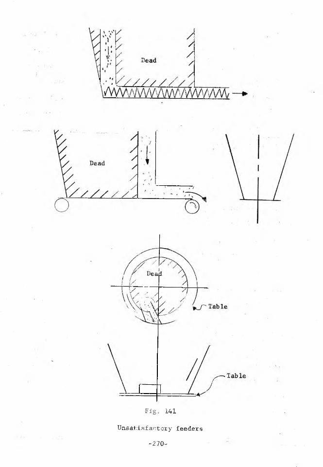
Fig, 141
Unsatisfactory feeders
-270“

Fig. 142
Satisfactory feeders!
-i7i-
The shape of the selected outlet will determine the type
of the feeder. In mass flow bins, the conditions of flow specify
only the minor dimension of the outlet. In plug flow bins^and in
storage piles for solids which do not pipe^because they are not
affected by consolidation at rest and their angle 8 is less than,
say, 50°, also only the minor dimension is specified. In those
bins the choice is open between a circular (or square) and an oblongS jshape of the outlet. The required diameter of a circular outlet
will usually be about twice the width of the oblong outlet but
other factors, like the cost of the bin, available headroom, plant
layout, conformity with other equipment in the plant, will bear
decisively on the selection of the type of feeder. Similarly,
for solids, whose flowability does not define a minimum dimension
and for which the dimensions of the outlet are determined from
considerations of particle interlocking or rate of flow, the choice
is open between a circular and an oblong outlet.
In plug flow bins and storage piles, for which both dimensions,
B and D, are specified by the conditions of flow, the dimension D is
always several times greater than B and an oblong outlet, or a slot,
is always more economical than a circular or square outlet.
Feeder loads. The vertical force Q which a flowing solid exerts
on a feeder can be estimated from eq. (103), in which m = 0 for plane
flow, m = 1 for conical flow; and the parameter q is read off the
appropriate chart, Figures 43 to 48. Only the values of 6 = 30°, 40°
and 50° have been plotted. For solids, whose 8 is larger than 50°J, the
-272-
computed-force is quite small and for them it is safer to use 5 = 50°.
For oblong outlets it is safe to use the plane-flow formula.
As an example: assume a hopper with conical walls inclined at an
angle 9' = 12°, angles 6' = 28°, 5 = 44°, T = 80 pcf, and an outlet
of diameter D = 1.5 feet. It is safe to use the chart for the lower
value of 8 = 40°, Fig. 47; the point (12°, 28°) specifies q = 0.20,
and eq. (.103) ,• with m = 1, yields Q = 0.20 x 80 x 1.5^ = 54 lb.
And another example: a hopper with a rectangular outlet 1 ft x 3 ft.,
side hopper slopes 9' = 25°, angles = 30°, 6 = 60°, and T = 110 pcf.
From Fig. 45, q = 0.35 and Q = 0.35 x 110 x 3 x l2 = 116 lb.
One conclusion is immediately apparent: these forces are very
small. They have been computed on the assumption that the feeder is
perfectly efficient, that no sliding of packed solid occurs. These
forces do not allow for the weight of the solid which would collect
in the pockets outside the hopper, Fig. 142, for the confining pressures
from the skirts, and for starting loads.
The starting loads on a feeder may be several times (a factor of
ten has been measured [31]) as much as the running loads. The reasons
are as follows: the low pressure which a solid exerts on a feeder :
during flow is due to the arching effect which develops within the
flowing solid and which causes most of its weight to be transferred
directly to the hopper walls. This occurs whenever the feeder is in
motion and the solid is flowing. When a solid is charged into an ;
empty bin while the feeder is at rest, there is no flow, arching at the
outlet of the hopper does not develop, a higher column of the solid
-273-
bears down on the feeder, and pressure is much higher. This situation
is often aggravated by the fact that, as the solid is charged into a
bin, its total weight increases, and the bin structure deflects. If
the feeder support is rigid and the feeder does not deflect in unison
with the bin, the feeder may take up a considerable part of the weight
of the bin and of the stored solid. Of course, as soon as the feeder
has started and flow in the bin has caused arching to develop, the
vertical force drops, but the initial force on the feeder may be....
very large. The peak loads are particularly detrimental to belt
feeders which rely on pre-tension for traction. In order to assure
traction during the peak loads, the pretension must be high, much
higher than is required during normal flow. This high tension contrib
utes to the loss of horsepower and to the wear of the feeder. These
starting peak loads can be eliminated by running the feeder whenever
the bin is being filled or, more positively, by providing a flexible
support for the feeder, for instance, a spring support.
' Belt feeder . The belt feeder, either flat or troughed, either
sliding on a plate (slide-belt feeder) or supported on idlers, provides
a simple and economical method of controlling the flow of solids from
slot outlets.
The belt feeder is especially well suited to solids which are fine
but do not aerate and flood (for instance, when charged into an empty
bin), and do not contain particles over 3/4" size. For these solids,
the hopper can be raised off the belt, a height of at least two largest
particle diameters and not less than 1/12 of the width of the outlet,
-274-
to provide a fully live outlet. Such a feeder will work satisfactorily
for outlet ratios L/B of 16 or more. A seal can be provided by outside
skirts.
The slide-belt feeder, Fig. 143, is low in first cost, reliable
and easy to maintain. The even surface of the belt, obtained by the
continuous support from the slide plate, tends to minimize the pressures
from the flowing solid and allows a tight seal at the skirts. Eq.(103)
is adapted to these feeders as follows
Q - 2q r L B(B + 0.2) (166)
B and L are measured in feet. The coefficient 2 is an overall safety
factor: it allows for the deviations of the actual flow pattern from
plane flow; which is used to calculate q (Figures 43 to 45), and for
the weight of the solid in the side pockets; whereas 0.2 specifically
allows for friction due to increased pressure as the solid flows side
wise under the hopper walls. This formula has been obtained from tests
run at the Flow of Bulk Solids Laboratory at the University of Utah.
If the outlet is tapered, an average width B provides sufficient
accuracy.
The component H of the belt tension necessary to draw the solid
is computed from the formula j
H = .45Q. . (167)
The frictional drag on the belt due to the slide plate, or rollers,
etc. must be added to H to obtain the net belt tension.
In order to relieve the peak loads on the feeder, the feeder
is supported on air or steel, springs which are computed as follows.
-275-
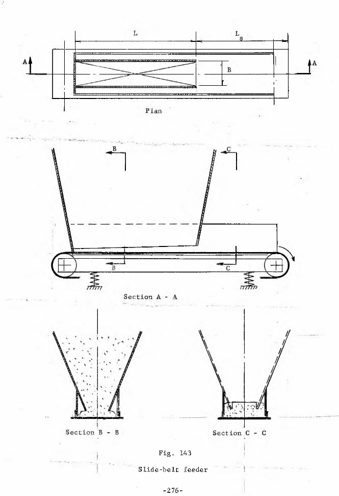
Fig. 143
Siide-belt feeder
-276-

Springs supporting a feeder
-277-

The total vertical load due to the feeder W is
W = Q + W d + W , , (168)
where is the dead weight of the feeder and W g is the weight of the
stream of the solid over the length L , outside the outlet. The total
spring constant (all springs in parallel) should be
C = 4Q lb/in9 (169)
.as shown in Fig. 144. The springs should be contracted under the
load W and locked so they can contract but cannot expand. In this
manner, the feeder will not start, deflecting until the load Q is
exceeded, and, under a peak load 2Q, the feeder will deflect 1/4 of
an inch. Laboratory tests show that a very small deflection, a few
hundredths of an inchs is usually sufficient to relieve the peak
loads. The feeder should be supported by links or guides in the
horizontal plane to prevent sway and to transfer the horizontal driving
force into the solid.
Laboratory measurements carried out on sand, gravel and iron ore
have shown that the velocity of the belt, within the tested range of
up to 80 feet per minute, does not appreciably affect the loads which
act on the feeder belt from the flowing solid.
Side-discharge reciprocating feeder. Reciprocating plate feeders
are well known and have been used over many years under square and
rectangular outlets. The ratio L/B of the outlets has been limited,
because the capacity of these feeders does not increase in the direction
of travel. An increase of the ratio L/B above 1.5 does not per
ceptibly widen the flow channel but greatly raises wear and power
-278-

requirements.
By changing the design of these feeders, they can be made especially
suitable for the feeding of unscreened coarse ore from storage piles.
Such ore is cohesive when moist, is often subject to changes of tempera
ture and to freezing„ As a result, it pipes around the outlets,
gradually packs in the non-flowing regions, and tends to dome. An
analysis of the flowability of such an ore usually gives some acceptable
value for the width of the outlet B, but the required diagonal of the
slot D, necessary to prevent piping, is very large and calls for a
continuous slot, running the full width (or length) of the storage
pile. The side-discharge reciprocating feeder is the most suitable
feeder for such a slot.
To the writer's knowledge there are no such feeders at present in
existence, therefore, the. description which follows anticipates their
application. A possible installation is shown in Figures 145 and 146.
The slot runs the full length of the storage pile. A gathering belt
conveyor runs in a tunnel alongside the slot. The slot is spanned
by cross-beams spaced at a distance t of 8 or 12 feet. Under each
length t there is a reciprocating feeder which discharges onto the
belt conveyor. The feeders can be suspended from above, as shown in
the figures, or supported from below. A flexible suspension is shown
to relieve the peak loads and to provide for impact. Vertical
walls separate the feeders so that each feeder can run independently
of the others.
The motion of the feeders must be coordinated with the speed of
.. -279-

« * • » < I • * --------------------» -
* * * K . _
Fig. 145
Layout of a side-discharge rsciprocating feeder under a pile
-280-

S 3 T 5 S 3 T
Section A - A
Fig. 146
Details of a side-discharge reciprocating feeder

the gathering belt. If n consecutive feeders spaced at t feet are
operating at a cycle of f strokes per minute, then the speed of the
belt v should be
v = f n £ ft/min, (170)
to obtain a fully loaded belt.
Another layout, which would be used to feed spearate mills, has
the slots and the gathering belt conveyors laid out across the pile,
as shown in Fig. 147.
Segregation and blending in flow
During the storage and handling operations, a bulk solid tends to
segregate (separate) according to the particle size, shape and density.
Since segregation is usually detrimental to the further processing and
merchandizing of the solid, the conditions leading to segregation,
means of minimizing segregation, and tnethods of remixing during flow
will now be described.
Most of the segregation takes place in the following two situations
when a solid flows in a freely falling stream which has a horizontal
component of velocity, and when the stream hits an inclined slope of
deposited solid. In free fall, each particle is acted upon by two
forces: its weight, and air resistance to motion. The former is
equal to the product of the size and the density of the particle, and
acts vertically down; the latter is a function of the size and shape
of the particle and of its velocity, and acts in the direction opposite
to the velocity. In vertical free fall, both these forces are vertical
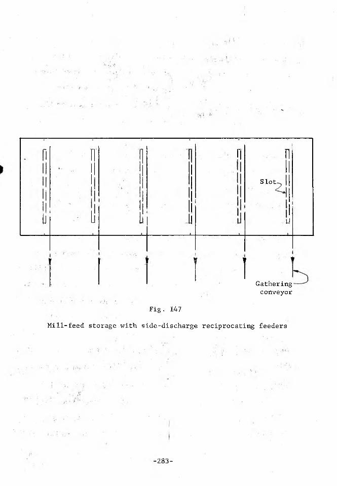
u
T'
I
! ij
!T nSlot
M
!Gatheringconveyor
Fig. 147
Mill-feed storage with side-discharge reciprocating feeders
283-

and, while the terminal velocities of the various particles may vary,
their trajectories do not, hence there is no significant segregation.
When a solid is discharged over a conveyor pulley or spouted through
an inclined chute aninitital horizontal component of velocity is
introduced, the two forces are not aligned any longer and, as their
ratios differ for the various particles, so do the trajectories of
the particles.
Whenever a stream hits a sloping surface, the particles roll down
the slope: the large, heavy, and more nearly spherical particles tend
to roll farther than the fine, light, and flaky particles which tend to
remain at the point of impact of the stream. As a pile of the solid
builds up, the fines congregate in a column which has the shape of the
trajectory; the size of the particles gradually increases with the
distance from the column, and the lumps collect at the periphery of
the pile or at the walls of the container. If the outlet of a pile
or of a plug-flow bin is located directly beneath the trajectory, the
draw will be heavily segregated: an excess of fines will be drawn
every.time the feeder is started after charging the solid while the
feeder was at rest. When the container has several outlets, the outlet
located under the trajectory will consistently draw an excess of fines.
This phenomenon can be exploited when some size separation is desired,
otherwise the outlets should be located away from the trajectory.
The aforesaid indicates that segregation is a dynamic effect and
occurs inevitably when the solid is in free fall. It also indicates
methods of minimizing segreation, which are: reducing the velocity of
-284-

the particles by shortening the height of free fall, reducing the hori
zontal component of velocity, and limiting the size of the slopes
along which the particles roll. The last method calls either for
narrow bins or for means to spread the stream over the top surface of
the container. Spreading can be accomplished either by placing a shelf
in the stream or by moving the point of discharge and the trajectory
of the stream. A combination of the two can be very effective in
minimizing segregation.
The degree to which a given solid will segregate under given condi
tions cannot yet be predicted quantitatively. Jenike [32] made a
preliminary study of the problem and suggests that a classification of
the solids^possibly, can be developed on the basis of simple tests which
would measure a ratio W/K, where W is the weight of a particle and K
is its resistance to motion through the air. He suggests that; parti
cles of the same ratio W/K will have little tendency to separate
from each other, and that the tendency will increase with a spread in
the values of the ratio. It would seem that the development of a quant
itative approach to the problem of segregation might benefit thiose who,
like the feed processors, handle and produce a variety of complex blends.V
When segregation in storage is to be avoided, a mass flow bin
should be used and the bin should be operated as explained in the 4th
'Example of design for flow1. Under these conditions first-in, first-
out flow obtains; while the solid segregates in charging, it remixes
within the hopper and, as a result, the blend of the draw is essentially
£he same as the blend of the charge.
. -285-

In slot-outlet bins charged by means of a tripper-conveyor, segre
gation is much smaller if the slots are perpendicular, Fig. 1.48(a),
than if they are parallel to the conveyor, (b), because in the former
case the slot draws a cross-section of the segregated solid which is
remixed on the feeder
In a multiple-out let bin, segregation is reduced by drawing
simultaneously through all the outlets and blending the draw.
A bin can be used for the blending of a solid by recirculating the
solid in a closed circuit, about the bin, provided the following con
ditions are satisfied: (a) the solid is non-segregating, e.g. it
is composed of uniform size, shape and density particles, or of very
small size particles; (b) a mass flow bin is used, so that there, are
no dead regions of the solid within the bin; (c) there is a substantial
velocity gradient in every horizontal cross-section of the channel, so
that first-in, first-out flow does not occur.
The above points (b) and (c) imply a bin with a short vertical
portion, whose height does not exceed one half the diameter of the cylin
der, Fig. 129, or no vertical portion at all. A higher vertical portion
would induce first-in, first-out flow and may cause dead-regions at the
transition.
A series of bins can be used to even out the grade of a run-of-mine
ore, Fig. 149, by charging the bins in sequence and drawing them '
simultaneously.
Flooding
Fine solids which aerate readily should be stored in mass-flow bins
• -286-
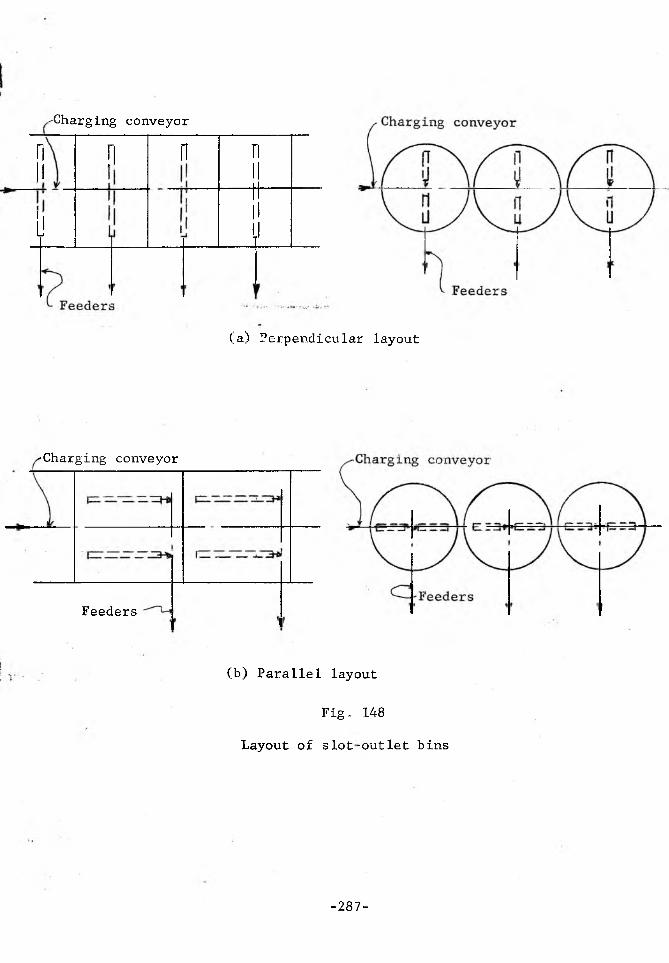
-Charging conveyor
nH
ii
FI II nII■tillII
(a) Perpendicular layout
-Charging conveyor
Feeders
(b) Parallel layout
Fig. 148
Layout of slot-outlet bins
-287-

in order to prevent flooding. In a plug-flow bin, flow is non-steady,
thick layers of the solid break away all at once, fall down the height
of the channel and aerate as they break up. Unless the feeder is
completely air-tight, flooding occurs.
Heat transfer
When flow of heat is to occur across the walls of a channel, the
channel should be of the mass-flow type, otherwise, the stationary
solid at the walls will act as an insulator between the flowing mass
and the walls. The channel should also be very steep so that the
velocity profile, defined in Fig. 68, and plotted, as an example, in
Figures 69 and 70 for & = 50°, be fairly uniform. If the velocity
is much higher at the center of the channel than at the walls, the outer
layers of the solid will undergo much more heating or cooling, as the(
case may be, than the core. To obtain a more uniform transfer of heat,
it is advisable to use a conical hopper with a pipe located at the
center of the channel and to use the pipe as well as the walls for the
transfer of heat. In general, the channels described in this work
are not efficient as heat exchanger because of the laminar flow patterns
of the solid.
Gas counterflow
In channels which serve as chemical reactors, a gas flows upwards
as the solid flows down by gravity. To cause the flow of the gas, a
pressure gradient is applied to it. This gradient opposes the forces
-288-
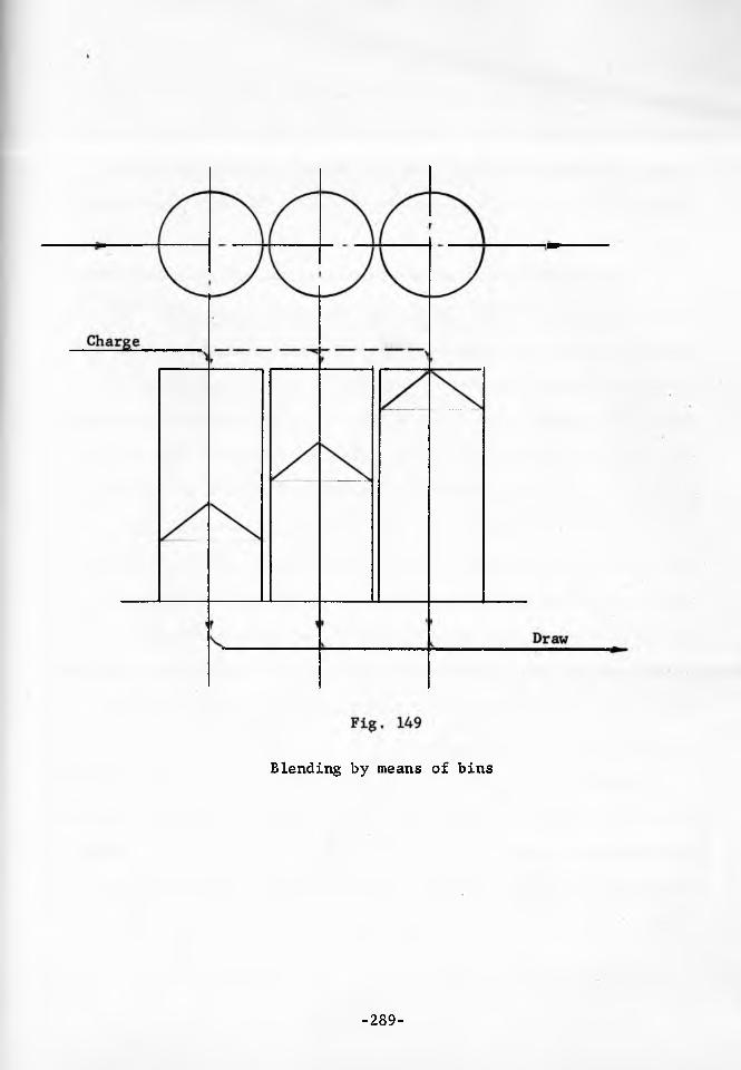
Blending by means of bins
-289-
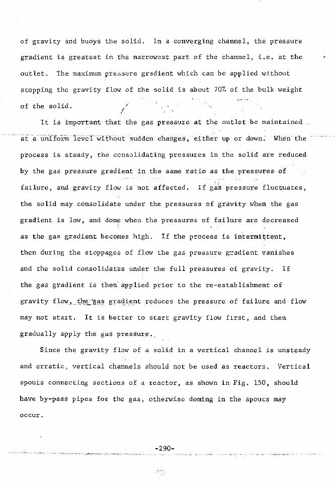
of gravity and buoys the solid. In a converging channel, the pressure
gradient is greatest in the narrowest part of the channel, i.e. at the
outlet. The maximum pressure gradient which can be applied without
stopping the gravity flow of the solid is about 70% of the bulk weight
of the solid. / , - ,/ i S . ' '
It is impoTrtant- that the gas pressure at the outlet be maintained ..
at a uniform level without sudden changes, either up or down. When the
process is steady, the consolidating pressures in the solid are reduced
by the gas pressure gradient in the same ratio as the pressures of !
failure, and gravity flow is not affected. If gas pressure fluctuates,
the solid may consolidate under the pressures of gravity when the gas
gradient is low, and dome when the pressures of failure are decreased
as the gas gradient becomes high. If the process is intermittent,
then during the stoppages of flow the gas pressure gradient vanishes
and the solid consolidates under the full pressures of gravity. If
the gas gradient, is then applied prior to the re-establishment of
gravity flow,, . thej'gas gradient reduces the pressure of failure and flow
may not start. It is better to start gravity flow first, and then
gradually apply the gas pressure.,
Since the gravity flow of a solid in a vertical channel is unsteady
and erratic, vertical channels should not be used as reactors. Vertical
spouts connecting sections of a reactor, as shown in Fig. 150, should
have by-pass pipes for the gas, otherwise doming in the spouts may
occur.
-290-
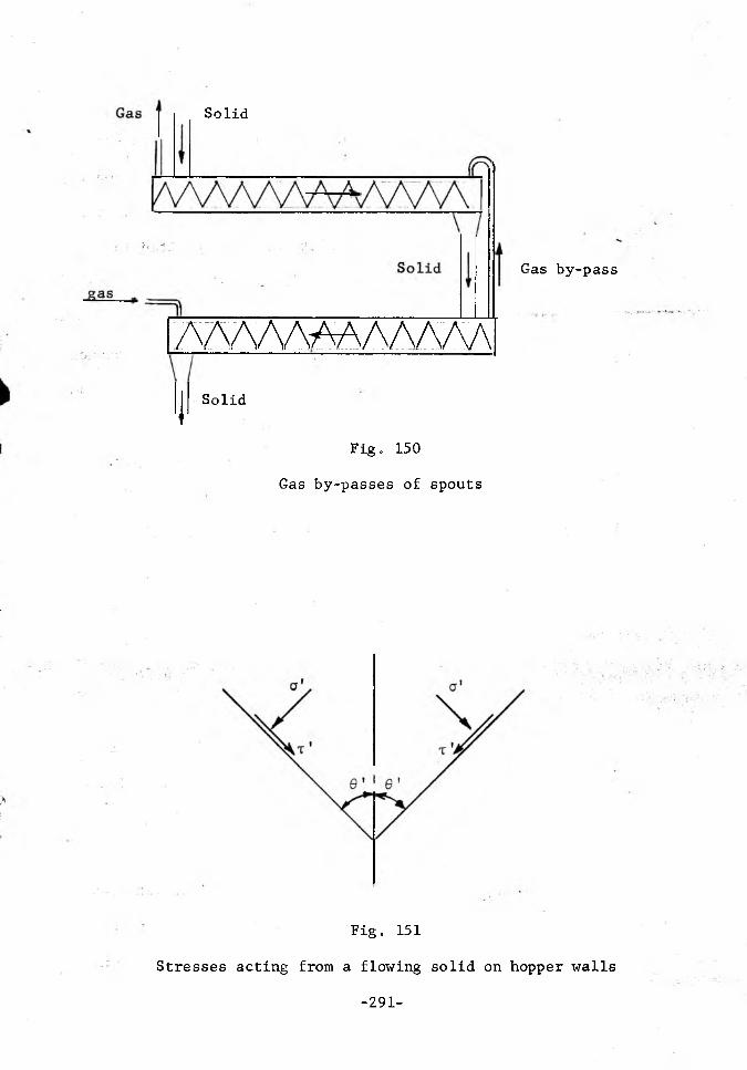
Solid
Gas by-pass
'AAAAAAAAAAM
'I'Solid
Fig. 150
Gas by-passes of spouts
Fig. 151
Stresses acting from a flowing solid on hopper walls
-291-

Structural problems
Stresses acting on hopper walls. The normal pressure a' and the
shearing stress -r' which a flowing solid exerts on the wall of a hopper,
Fig. 151, have been computed for symmetric hoppers in plane and conical
flow. Contours of constant values of these stresses are plotted in
Figures 50 to 61 for the values of 5 = 30°, 40°, and 50°. The stresses
for 5 > 50° are less than those for 6 = 50°.
It will be observed that these stresses are very low. For instance
in plane flow, 5 = 40°, 0' = 15°, i 1 = 23°, V = 100 pcf, B = 2 ft., from
Fig. 51, a' = 1.01 x 100 x 2 = 202 psf, which is equivalent to a static
head of the solid of 2.04 ft, or just about the width of the hopper.
In conical flow, these stresses are less yet; for instance, for the
same 0', 4>' , X and B, from Fig. 54, a' = .50 x 100 x 2 = 100 psf.
For easy, and free-flowing, fine solids the above values are
acceptable for design purposes. For cohesive solids, which can dome
and impose large impact loads upon failure, and for solids containing
large particles, a safety factor needs to be used over the computed
values.
It should be remembered that these values have been derived for
mass flow and in cases of plug flow can only be used as a guide. The
stresses on the hopper will also be higher in the vicinity of the
transition to the vertical portion. x
Bin failures. Failures of bin structures can be divided into two
categories. In the first category belong those failures which are due
to recognized structural causes, such as: foundation failure, uneven
-292-
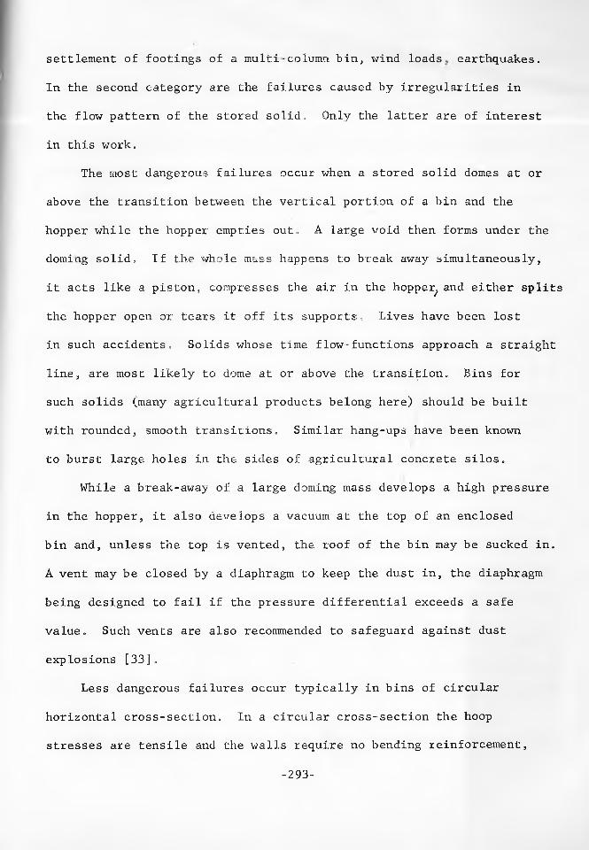
settlement of footings of a multi-column bin, wind loads,, earthquakes.
In the second category are the failures caused by irregularities in
the flow pattern of the stored solid. Only the latter are of interest
in this work.
The most dangerous failures occur when a stored solid domes at or
above the transition between the vertical portion of a bin and the
hopper while the hopper empties out. A large void then forms under the
doming solid. If the whole mass happens to break away simultaneously,
it acts like a piston, compresses the air in the hopper^ and either splits
the hopper open or tears it off its supports. Lives have been lost
in such accidents. Solids whose time flow-functions approach a straight
line, are most likely to dome at or above the transition,, Bins for
such solids (many agricultural products belong here) should be built
with rounded, smooth transitions. Similar hang-ups have been known
to burst large holes in the sides of agricultural concrete silos.
While a break-away of a large doming mass develops a high pressure
in the hopper, it also develops a vacuum at the top of an enclosed
bin and, unless the top is vented, the roof of the bin may be sucked in.
A vent may be closed by a diaphragm to keep the dust in, the diaphragm
being designed to fail if the pressure differential exceeds a safe
value. Such vents are also recommended to safeguard against dust
explosions [33].
Less dangerous failures occur typically in bins of circular
horizontal cross-section. In a circular cross-section the hoop
stresses are tensile and the walls require no bending reinforcement,
-293-

provided the stresses acting on the walls from the solid are uniform
all-around. This condition is satisfied if the solid is charged and
drawn at the center of the bin. Therefore, the hopper, if any, must
be circular and symmetric with respect to the vertical axis: only one
outlet is permitted. If the hopper is offset to one side, Fig. 152, the
pressures from the solid on the vertical side are decreased and the
hoop stresses in the hopper may pull that side in. Bending reinforce
ment is required to retain the shape of this hopper.
In a cylindrical, flat-bottom bin with two (or more) outlets, Fig.
153, the solid empties out of two craters centered at the outlets and
the pressures on the walls at points A fall to zero while, simultaneously,
at B the solid presses against the walls. As a result, the walls at
A are pulled in. To counteract this effect, the cylinder should be
reinforced by rings between the A and B levels.
Ores
Broken rock. From the stand point of flow, the main character
istic of these solids is the large size of the rocks compared to the
cross-section of the channels through which the rock has to flow. In
most ore passes, chutes, and ore pocket outlets, the dimensions of the
apertures are well below those plotted in Fig. 123, hence the probability
of interlocking is substantial. However, experience shows that flow is
sufficiently reliable provided the smaller dimension of the aperture, a^is
a > 2d, . (171)
where d is the intermediate dimension of the largest rocks, Fig. 154.

-295-

It is interesting to note that the largest dimension of the rocks does
not enter into this formula. This is explained by the fact that, when
ever a solid flows in an even slightly converging channel, the velocity
profile is as shown in Fig. 155. If a rock of length t happens to be
positioned as shown at A, its velocity v^ at one end is greater than
v^ at the other end, and the rock rotates as it flows, until it has
aligned in the direction of flow, as shown at B.
From the standpoint of flow, an ore pass should be converging and
not straight. Flow in a converging channel is more steady, the pressures
in the solid are lower and, hence, the consolidation and the tendency
for doming is less.
In a straight channel, flow is non-steady, therefore pressures
are higher, the solid does not converge but flows like a rigid plug and,
even though it flows, it undergoes consolidation at rest under these
higher pressures, resulting in increased tendency for doming. Beside
that, flow in a straight channel causes more wear at the walls. This
can be illustrated by the consideration of the energy of a flowing
mass. As the solid flows down, it dissipates by friction the potential
energy due to the gravitational field. In a straight channel, the
solid flows like a rigid plug and all the energy is dissipated at the
walls, wearing out the wall surfaces. In converging flow, the shape of
the flowing mass is continuously changed, and a part of the work is
done within the solid itself, reducing the energy spent at the walls.
The pattern of flow in an ore pass is governed by its shape at the
outlet and the method of controlling the draw. The principle of the
-296-

W V / A \ ^
Fig. 154
Cross-section of an ore pass
-297-
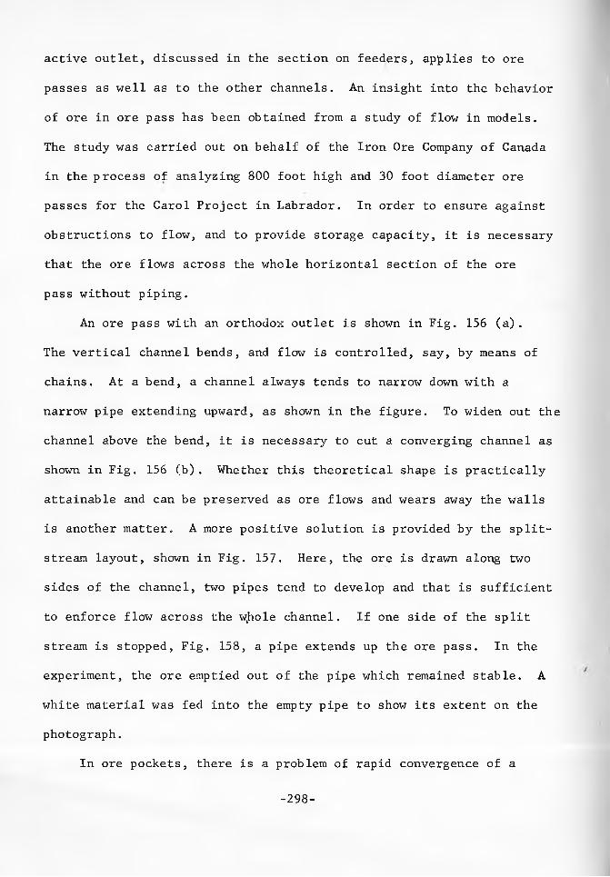
active outlet, discussed in the section on feeders, applies to ore
passes as well as to the other channels. An insight into the behavior
of ore in ore pass has been obtained from a study of flow in models.
The study was carried out on behalf of the Iron Ore Company of Canada
in the process of analyzing 800 foot high and 30 foot diameter ore
passes for the Carol Project in Labrador. In order to ensure against
obstructions to flow, and to provide storage capacity, it is necessary
that the ore flows across the whole horizontal section of the ore
pass without piping.
An ore pass with an orthodox outlet is shown in Fig. 156 (a).
The vertical channel bends, and flow is controlled, say, by means of
chains. At a bend, a channel always tends to narrow down with a
narrow pipe extending upward, as shown in the figure. To widen out the
channel above the bend, it is necessary to cut a converging channel as
shown in Fig. 156 (b). Whether this theoretical shape is practically
attainable and can be preserved as ore flows and wears away the walls
is another matter. A more positive solution is provided by the split-
stream layout, shown in Fig. 157. Here, the ore is drawn along two
sides of the channel, two pipes tend to develop and that is sufficient
to enforce flow across the w.hole channel. If one side of the split
stream is stopped, Fig, 158, a pipe extends up the ore pass. In the
experiment, the ore emptied out of the pipe which remained stable. A
white material was fed into the empty pipe to show its extent on the
photograph.
In ore pockets, there is a problem of rapid convergence of a
-298-
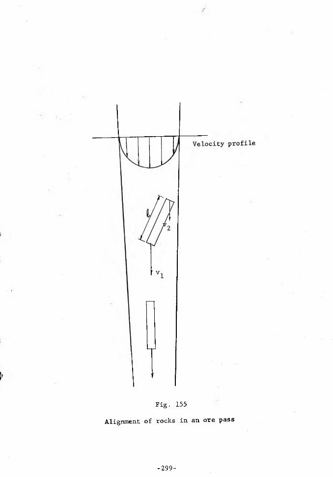
Fig. 155
Alignment of rocks in an ore pass
-299-

Orthodox shape ...... . .. .. Preferred shape.
Fig. 156
Outlets of an ore pass
-300-

channel toward and within a feeder, as shown in Fig. 159. In this case,
a successful operation requires that, at any particular cross-section
of the channel, convergence by in one plane only. The walls and the
skirts of the ore pocket are so shaped that^within its upper part^
flow converges only in plane z - x, in the intermediate part, only
in plane y - z, and at the outlet, only in plane x - y. Since the
pocket is to handle rock up to a 5 foot intermediate dimension onto
a 7 foot apron feeder, it is important that one side wall slopes all
the way down to the feeder. This brings the narrow part of the hopper
to within the range of action of the feeder and allows it to disturb
any large boulders which may tend to interlock.#
Coarse ore (minus 8 inch) which contains fines and a high moisture
content is difficult to store and to feed. The difficulties are
aggravated when frozen ore is charged into storage and, even more so
during fall and spring, when the charged ore is partly thawed out during
the day and refreezes in storage at night.
Under these conditions the best solution is to keep as much of
the ore as possible in a live, flowing state. The velocities of flow
need not be high to prevent the ore from freezing and from consolidation
at rest. This solution will be obtained most economically by providing
long, active slot-outlets with side-discharge reciprocating feeders,
Figures 145 to 147.
# The author is indebted to the engineers at Carol who built a model of such an ore pocket, proportioned it for best flow, and demonstrated its advantages. The mining operation is due to start in the summer of 1962.
-301-

Fig. 157
Model of a split-stream ore pass drawing at both sides
-302-
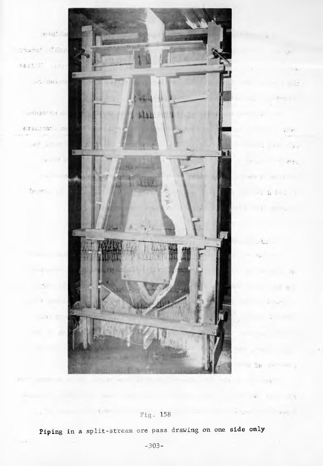
Fig. 158
Piping in a split-stream ore pass drawing on one side only
-303-
It should be remembered that, as a coarse ore is charged into
storage, the large lumps hit the deposited mass with considerable impact
and pack it severely along the trajectory of the falling stream. Unless
the ore is free flowing, it is advisable to spread the stream and to
distribute the impact over a wide area. ‘
An alternative solution is available when the ore can be screened
into a coarse and a fine (say, below 1/2") fraction. The two fractions
are then handled separately. The coarse fraction is free flowing and
can be stored in flat bottom bins or storage piles and drawn from
storage by means of standard reciprocating feeders, apron feeders,
or fed directly onto belt conveyors. The fine fraction can be stored
in mass flow bins with slot outlets and belt feeders.
Block-caving
In the mining operation of block-caving, a number of draw points
is located in tunnels beneath the ore body and a sufficient volume of
the ore above the draw points is shattered to cause the whole body
to break-up and flow by gravity into the draw points. The ideal flow
pattern, which is aimed at, is a uniform drop of the whole ore body
without piping. The flow pattern is governed by the location of the
draw points, the shape of the crater of the initial shatter, and the
sequence of draw.
Considering the flow channel above a draw point, it is evident that
the most favorable crater would be a circular cone which would produce
a regular channel with weak walls and of an included angle 20',
-304-
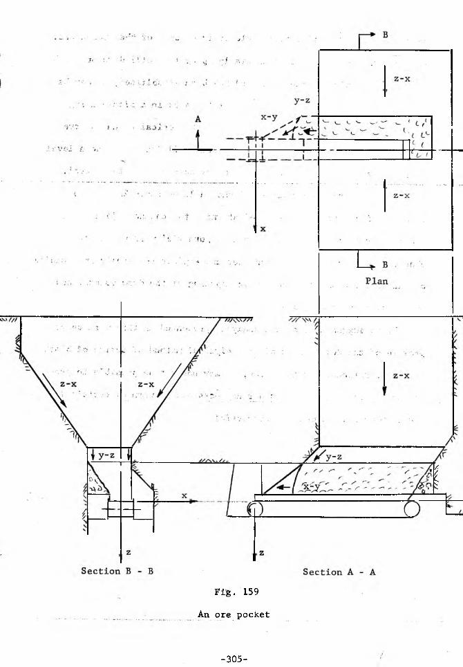
Fig. 159
An ore pocket
-305-
/"A
nn
appropriate for the effective angle of friction 8 of the broken ore.
If too much ore is shattered initially, plug flow will develop with
inevitable piping. Once a channel has been established, it may be
impossible to alter it. Thus, the first blasts in a block-caving
operation may decide of its success. If the conical channels have
formed above the draw points, the channels will jo£n up at some level
w ithin the ore body and uniform flow may obtain above that level.
The spacing of the draw points and the included angle 26' of the
channels will determine the level at which the channels join up.
Since every fault in the ore body is a potential weak plane for a
channel, it is necessary to consider and exploit the faults in deciding
on the most economical location and spacing of the draw points, and
on the slope of the channels.
It is suggested that the analysis presented in this work shows
promise of the development of an analytical method of design of block-
caving operations. At this time, it may not yet be possible to prescribe'
an optimum layout, but it is already possible to warn of certain layouts
and methods which cannot be successful. '
-306-

REFERENCES
1. Sokolovski, V. V., Theory of Plasticity, Government Printing House of Technical and Theoretical Literature, Moscow, 1946.
2. Prager, W. and Hodge, P. G., Theory of Perfectly Plastic Solids, Wiley, New York, 1951.
3. Hill, R. , The Mathematical Theory of Plasticity, Oxford, 1950.
4. Sokolovski, V. V., Prikl. Mat. Mekh., 1950, Jiy, 75.
5. Shield, R. T., J. Mech, Phys. Solids, 1955, _3, 246.
6. Von Mises, R. , Z. angew. Math. Mech., 1928, 8, 161.^ - . -
7. Drucker, D. C., Proc. 1st U. S. Nat. Cong. Applied Mechanics, 1951, 487.
8. Haithornthwaite, R. M., J. Soil Mechanics Fndn. Div.. Proc.Amer. Soc. Civ. Eng.. 1960, 8£, 35.
9. Jenike, A. W., and Shield, R. T., J. Appl. Mech., 1959, 81B, 599.
10. Shield, R. T., J. Mech. Phys. Solids, 1955, 4, 10.
11. Drucker, D. C., Gibson, R. E., and Henkel, D. J., Trans. Amer. Soc. Civ. Engr., 1957, 122, 338.
i ■ ■ i i i i w ■» ' / W S V
12. Haar, A. and von Karman, Th., Nachr. Ges. Wiss. Gottingen, Math.- Phys., Kl. 1909, 204.
13. DeJosselin DeJong, G., Statics and Kinematics in the Failable Zone of a Granular Material, Uitgeverij, Waltman - Delft, 1959.
14. Jenike, A. W., Elsey, P. J. and Woolley,R. H., Flow Properties of Bulk Solids, Utah Engrg. Exper. Station, University of Utah, Bui. 95, 1958.
15. Sokolovski, V. V., Statics of Soil Media, English translation, Butterworths, London, 1960.
-307-
16. Jenike, A. W., Flow of Bulk Solids, Utah Engrg. Exper. Station, University of Utah, Bul„ 64, 1954.
17. Jenike, A. W . , Chem. Engrg., 1954, 61, 175.——----- w /WA.18. Shield, R. T., Quarterly Appl. Math., 1953, JTL, 61.
19. Cox, A. D., Eason, H. G. and Hopkins, H. G., Axially-symmetric Plastic Deformations in Soils, A. R. D. E. Report (B) 14/58,Ministry of Supply, Fort Halstead, Kent, England, 1958.
20. Cox, A. D., Axially-symmetric Plastic Deformations in Soils II - Indentation of a Plane Surface by a Circular Cylinder, A. R. D. E. Report (B) 22/59, The War Office, Fort Halstead, Kent, England, 1959.
21. Cox, A. D., Axially-symmetric Plastic Deformations in Soils III - Indentation of Ponderable Soils, A. R. D. E. Report (B) 16/60,The War Office, Fort Halstead, Kent, England, 1960.
22. Jenike, A. W. and Yen Bing Cheng, Slope Stability in Axial Symmetry, Utah Engrg. Exper. Station, Univ. of Utah, Bui. 115, 1962.
23. Johanson, J. R. and Jenike, A. W., Stress and Velocity Fields in Gravity Flow of Bulk Solids, Utah Engrg. Exper. Station, Univ. of Utah, Bui. 116, 1962. '
24. Ketchum, M. S., The Design of Walls, Bins and Grain Elevators, Mc-Graw Hill, New York, 1919.
25. Mitchell, D. R., Trans. Amer. Inst. Mining Eng., 1938, 130, 107.
26. J. R. O'Callaghan, J. Agric. Engrg. Research., Wrest Park, Bedfordshire, England, 1959, ^ 200.
27. Colburn, A. P., Industrial and Engineering Chemistry, 1931, 23, 913.
28. Shedd, C. K., Agricultural Engineering, 1951, 32, 493.
29. Shedd, C. K., Agricultural Engineering, 1953, 34, 616.
30. Sinden, A. D., Getting "Difficult" Materials out of Bins", The Amer. Soc. Mech. Engr., paper 61-BSH-8.
-308-
31. Jenike, A. W., Elsey, P. J. and Woolley,R. H., Flow of Bulk Solids - Progress Report, Utah Engrg. Exper. Station, Univ. of Utah, Bui. 96, 1959.
32. Jenike, A. W., A Preliminary Study of Segregation, Utah Engrg. Exper. Station, Univ. of Utah, Bui. 107, 1960.
33. Olson R. W., Mechanical Engineering, 1961, 8^, 59.
-309-