building scal capacity in developing countries: evidence on the … · 2019-04-11 · building scal...
TRANSCRIPT

Building fiscal capacity in developing countries:Evidence on the role of information technology
Merima Ali∗, Abdulaziz B. Shifa†, Abebe Shimeles‡, Firew Woldeyes§
June 1, 2018Abstract
Weak fiscal capacity for domestic resource mobilization is considered asone of the most important challenges in poor countries. Recently, manydeveloping countries resorted to the application of information technologyto consolidate tax mobilization; however, there is little systematic empiricalevidence on the impact of such reforms. We attempt to narrow this gapby providing evidence from Ethiopia where there has been a recent surgein the adoption of electronic sales register machines (ESRMs). We use aunique administrative firm-level panel data covering all business taxpayersin Ethiopia and apply matching difference-in-difference method to accountfor possible bias that may arise due to selection. We find that adoptionof ESRMs has a significant positive effect on tax payments and reportedsales. Moreover, we find a positive effect on employment and no effect onnet entry, suggesting that increased tax payments by registered taxpayersoccurred without erosion of the tax base.
JEL Classification: H26, H32, O10, O55Keywords: Developing economy; fiscal capacity; information technology; taxation.
1 Introduction
Economic development requires a state capable of mobilizing fiscal resources to fi-nance the provision of essential public goods—a capacity that developing countriestend to lack. Weak fiscal capacity of states has thus received increased attentionin the political economy of development.1 Governments with the bare minimumof a tax administrative infrastructure, as is typical of developing countries, find itdifficult to enforce tax compliance partly due to lack of reliable records on earn-ings by taxpayers. Thus, the potential that information technology (IT) affordedto gather and analyze large amounts of data on taxpayers at relatively minimalcost has caught the attention of tax authorities throughout developing countries.Tax reform efforts to enhance monitoring earnings and improve tax collection “in
∗CHR Michelsen Institute and Syracuse University. Email: [email protected]†Maxwell School, Syracuse University. Email: [email protected]‡African Development Bank. Email: [email protected]§Ethiopian Development Research Institute. Email: [email protected], for example, Bird, 1989; Tanzi and Zee, 2000; Acemoglu, 2005; Besley and Persson,
2010, 2011; Baskaran and Bigsten, 2013.
1
developing countries have generally centered on information technology” (Bird andZolt, 2008, pp. 794). Nevertheless, there has been little, if any, systematic empir-ical evidence on the impact of those reforms. In this study, using administrativefirm-level panel data on a large number of business taxpayers, we provide evidenceon the impact of using the electronic sales register machines (henceforth, ESRMs)on tax revenues in the context of a developing country.
The focus of our study is a recent reform to expand the use of ESRMs inEthiopia—a sub-Saharan African country with one of the lowest per capita incomesin the world and a minimal fiscal capacity. Starting in 2008, the Ethiopian Revenueand Customs Authority (ERCA) required several businesses to use ESRMs. Theprogram has been rolled out over many rounds, and in 2014, over 60,000 firmsadopted the new system to conduct business transactions. The machines registersales and print receipts. The transactions are then reported via a network to anERCA server. Hence, once a firm starts using ESRMs, ERCA receives daily dataon the firm’s revenue. This provides ERCA with the ability to monitor reportedrevenues on a daily basis. With the traditional, paper-based receipts, this wouldhave been prohibitively expensive and virtually impossible.
Even though ESRMs have the potential to provide more accurate transactiondata to help minimize tax evasion, it is not clear whether developing countriescan effectively harness ESRMs to generate higher tax revenues. First, develop-ing countries may face technical and administrative challenges in implementingESRMs. Operation of the machines requires a reliable supply of electricity andnetwork infrastructure, as well as availability of technical capacity that can ad-minister the network. In addition, processing of the massive data collected to aiddecision-making would not be an easy fit, given the lack of requisite technical ex-pertise and coordination failures among public agencies. Moreover, the machinesdo not enforce tax rules by themselves; they merely provide information on rev-enues. Whether the information is utilized to improve tax compliance depends onadministrative and legal factors, as well as perception by businesses of the credibil-ity of the threat posed by the new technology in terms of increasing oversight. Forexample, business owners may still evade taxes by paying bribes to tax officers,who would otherwise use the new set of data to track evasions. Thus, in settingswhere institutions are weak, as is typically the case in developing countries, theimpact of gaining extra information on earnings may be minimal.
Second, even if ESRM adoption leads to increased enforcement among reg-istered taxpayers, the overall effect on tax payments may go in either directiondepending on how ESRMs affect the tax base. On the one hand, increasing taxeson final sales may lower demand, decrease production, and encourage exit out of(or discourage entry into) the formal sector. This effect implies that ESRMs canlead to erosion of the tax base. On the other hand, ESRM adoption may affectthe decision of firms in a way that incentivizes them to operate at larger scales,hence expanding the tax base. For example, in the absence of ESRM adoption,evading taxes may require firms to operate on a smaller scale. This would be thecase if, as firms become larger, they tend to leave easily detectable traces thatmake tax evasion harder, thereby encouraging the firms to remain small. How-
2

ever, if the adoption of ESRMs leads to more accurate revenue records irrespectiveof firm’s scale of operation, firms may no longer have the incentive to perate insmaller scale in order to evade taxes. The adoption of ESRMs, by helping improvebusiness records, may also have a direct effect on the firm’s output and employ-ment. This could happen if ESRMs help firms lower the cost of supervising theiremployees, making it easier for entrepreneurs to delegate tasks and expand theirscale (Akcigit et al., 2016).
Hence, in order to provide a fuller picture of the effect of ESRMs on overallfiscal capacity, we empirically examine the impact of ESRMs on both tax pay-ments by registered-taxpayers and proxies of the tax base. In order to accountfor possible bias that may arise due to selection into ESRM adoption, we usematching difference-in-difference (MDID) method. MDID has increasingly beenused in the evaluation literature to address endogeneity concerns in studies usingnon-experimental data (Girma and Gorg, 2007; Becerril and Abdulai, 2010).
We find three major patterns in the data. First, firms report higher salesand pay more value-added tax (VAT) following ESRM adoption. Second, as aproxy for the effect of ESRM adoption on the tax base, we look at the effect onemployment and rates of net entry into the formal sector. Rates of net entry isdefined as the number of newly entered firms minus those that exited, as a share ofthe existing firms. We find that employment increases following ESRM adoption,suggesting that firms did not decrease their production in response to ESRMadoption. Furthermore, differences in rates of ESRM adoption across sectors orlocations are not found to be associated with rates of net entry into the formalsector. In summary, the fact that reported sales and tax payments increasedwithout lowering either employment or net entry suggests that ESRMs helpedenhance overall fiscal capacity.
This paper contributes to the growing literature on the fiscal capacity of thestate and tax compliance in developing countries. One of the important challengesfor tax authorities in developing countries is the lack of accurate information onearnings (Jenkins and Kuo, 2000; Engel et al., 2001; Fisman and Wei, 2004; Boad-way and Sato, 2009; Gordon and Li, 2009; Olken and Singhal, 2011). This moti-vated a number of recent studies that assessed alternative policy tools to providetax authorities with more reliable information (see, e.g., Slemrod, 2008; Kumleret al., 2013; Naritomi, 2016; Carrillo et al., 2014; Pomeranz, 2015; Slemrod et al.,2017). Even though governments in many developing countries are expanding theadoption of electronic tax system to enhance their ability to gather, analyze, andmonitor earnings information, we are not aware of any study examining the impactof electronic tax systems in the context of developing countries—a gap that ourstudy attempts to narrow.
This paper is also related to the literature on the impact of IT on economicoutcomes. These studies have mostly focused on the effect of IT on private sectorproductivity (Brynjolfsson and Hitt, 2000; Bresnahan et al., 2002; Stiroh, 2002).Despite the widespread adoption of IT in public service delivery, commonly knownas “e-governance,” assessment of the impact remains relatively unexplored (Gari-cano and Heaton, 2010). Two recent seminal contributions are Lewis-Faupel et al.
3

(2016) and Muralidharan et al. (2016), who studied the impact of IT use on publicservice delivery in the context of developing countries. Using evidence from India,Muralidharan et al. (2016) study the impact of using biometrically-authenticatedpayment systems on the effective delivery of targeted social transfer payments.Lewis-Faupel et al. (2016) documented the impact of electronic procurement oninfrastructure provision in India and Indonesia. Our paper contributes to thisstrand of literature on IT and state capacity building in developing economies.
Research on the impact of tax reforms in developing countries is quite limiteddue to the lack of accurate data on tax payments. Our paper contributes tothe few, but significant, advances that have recently been made in the use ofadministrative tax data from developing countries to study tax reforms (see, e.g.,Kleven and Waseem, 2013; Best et al., 2015).
The paper is structured as follows. In Section 2, we discuss the institutionalbackground of taxation in Ethiopia and describe the data. The empirical analysisproceeds in three steps. First, we report the preliminary results on the impact ofESRMs on reported sales, VAT, and employment (in Section 3). Then, we com-plement the preliminary results using evidence from matching diff-in-diff analysis(Section 4). Finally, we present results on the impact of ESRMs on net entry(Section 5). Concluding remarks follow in Section 6.
2 Background, data and outline of the empirical
analysis
2.1 Background and Data
Our data set comes from Ethiopia—a country that was ravaged by a long civilwar during the Cold War era and still remains one of the poorest countries insub-Saharan Africa. In 2010, Ethiopia’s GDP per capita was about 1,000 USD incurrent purchasing power parity. For comparison, this figure is only about one-third of the average in sub-Saharan Africa and less than one-thirtieth of the OECDaverage.2
The need for fiscal resources was no more apparent than in the lack of basicpublic infrastructure, such as roads that are needed to connect the markets acrossthe country. However, as is the case with many developing countries, Ethiopiahas a low level of fiscal capacity. The tax revenue, as a share of GDP, was about12% during the decade 2001-2011. Ethiopia also relied heavily on taxes on in-ternational trade—a kind of tax that is relatively easy to enforce but tends tobe more distortionary to the economy. More than 40% of Ethiopia’s tax revenuecame taxes from international trade—a very high ratio even by the standards ofdeveloping countries. About a third of the revenues came from income taxes.
Against this background, the government undertook two major reforms thatare the focus of this study. The first one was the introduction of the VAT, which
2The per capita GDP for OECD, Sub-Saharan Africa and Ethiopia, respectively, are 34,483,3,056 and 1041 (WDI online data bank, accessed on July 13, 2014).
4

is a main outcome variable in our paper. VAT was introduced in 2003 with theaim of broadening the domestic tax base and minimizing the dependence on tradetaxes. VAT has become a significant source of government revenue contributingnearly one-fifth of domestic total tax revenue and half of indirect tax revenue.Since its introduction, the VAT rate has been set at 15%. The second reformwas the adoption of ESRMs in 2008. By maintaining electronic record of businesstransactions, ESRMs are meant to minimize tax evasion by businesses.
Given the logistics challenges in implementing these reforms all at once, VATregistrations and ESRM adoptions were rolled out gradually. The rollout happenedthrough a series of ad hoc directives issued by ERCA that made it mandatory foran increased number of firms to enroll in the reforms. The solid line in Figure 1plots the number of VAT-registered taxpayers and ESRM users. VAT registrationstarted with about 6,000 firms in 2003, gradually expanding, to reach over 140,000firms by the end of 2014.3 The adoption of ESRMs began with a few hundred firmsin 2008. By 2014, about 73,000 taxpayers (out of over 140,000 VAT-registeredtaxpayers) adopted ESRMs4.
Our data-set contains administrative tax records on the universe of VAT-registered firms in Ethiopia, both ESRM users and non-users (see Figure 1). Theadministrative records provide information on several factors such as sales, em-ployment, VAT payments, location, types of business activity (sector), ownershipstructure, age and date of ESRM adoption. We have data covering the period fromJanuary 2003—the year of VAT introduction in Ethiopia—to the end of 2014. Thedata series are available on monthly frequency.
Table 1 presents some key characteristics of the firms in our sample. These firmsare mostly businesses located on main streets across major cities in the country.Nearly half of the firms are from the capital city (Addis Ababa). Majority of thefirms operate in the service sector. About 35% of the firms engage in retail, mostlyrepresenting shops on major city streets. About 20% of the firms are non-retailservices, including services such as beauty salons, coffee shops, jewelry makers andso forth. Another 15% of the firms are from the construction sector, which hasbeen booming in Ethiopia over the past years.
Most of the firms are family-run small-scale businesses that are typically single-outlet stores in cities, as indicated by a relatively high share (67.5%) of owner-operated firms, i.e. firms that did not report formally hiring outside labor. Ofthose who hired outside labor, the average employment stands at 54.6. However,the median employment is only 2.6 number of workers, implying that most of thefirms are quite small.5
3The legislation for VAT registration exempted smaller firms. For a detailed theoreticaldiscussion on the optimal VAT threshold, see Keen and Mintz (2004).
4As has been the case for VAT registration, smaller firms were not required to adopt ESRMsdue to cost. According to our conversations with ERCA officials, the machines typically cost5,000 to 13,000 Birr (about 250 to 650 USD in current market exchange rate), a significantexpense for many businesses in Ethiopia. Once ERCA decides that a firm should use ESRM,the machines are installed at the firm’s sales outlets/stores. This is done in the presence of ITtechnicians from ERCA who assess whether the installations satisfy the technical requirementsand standards set by ERCA.
5This situation of firm distribution where the economy is dominated mostly by small firms
5

Figure 1: Number of VAT payers and ESRM adopters (’000).
6.513.1
17.922.4 26.3
31.239.2
50.4
73
99.7
121
140.4
.3 1.19.3
30.1
46.7
61.8
72.8
050
100
150
'03 '04 '05 '06 '07 '08 '09 '10 '11 '12 '13 '14Year
All Tax Payers ESRM users
On average, annual sales and VAT collections are 884,411 Birr and 112,223Birr, respectively.6 By the end of 2014, nearly half of the firms adopted ESRMs.We provide detailed comparisons between firms that adopted ESRMs and thosethat did not. These comparisons are reported in Tables A1–A4. We discus thesecomparisons in our matching analysis (Section 4).
2.2 Outline of empirical analysis
As discussed in the introduction, our focus is on the impact of ESRMs on overalltax capacity. ESRMs may affect tax capacity in two possible ways. First, byaltering revenue data available to the tax authority, ESRMs may affect compliancebehavior among registered taxpayers. This would be the case, for example, ifESRMs increase the cost of tax evasion (by increasing the likelihood of detection),hence improve compliance. Second, ESRMs may affect the tax base depending onhow firms respond to ESRM adoption. For instance, if ESRMs lead to increasedtax compliance, firms may respond by exiting from the formal sector (to shunESRM adoption). The increase in tax payments may increase overall cost ofproduction and hence induce firms to lower their output. As a result, ESRMs
is consistent with the broad pattern in developing countries (Hsieh and Olken, 2014). The highstandard deviation in sales, VAT and employment in table one is also due to the large share ofsmall firms in the economy
6With the nominal exchange rate of about 20 Birr/USD, these amounts correspond to 44,225and 5,611 USD, respectively. The numbers are not adjusted for inflation.
6

Table 1: Descriptive statistics
Mean Std. Median
Addis Ababa (dummy for located in Addis Ababa) 0.48 0.50 —Sectors:
Retail 0.35 0.48 —Non-retail services 0.20 0.40 —Construction 0.14 0.35 —Others 0.31 0.46 —
Owner-operated 0.68 0.49 —Annual sales (’000 Birr) 884.41 3, 467.37 69.52Annual VAT (’000 Birr) 112.22 459.10 7.92Employment 54.64 2286.39 2.67Adopted ESRM by 2014 (share) 0.48 0.50 —
The table presents descriptive statistics for 153,825 firms in our sample. We report the share offirms in Addis Ababa, the share of firms in each listed sectors, the share of firms operated by theirowners (i.e. firs that hire no outside labor), mean annual sale, mean annual VAT, employmentamong non-owner operated firms and share of firms that adopted ESRMs by the end of 2014.
may lead to erosion of the tax base. In order to assess the effect of ESRMs onoverall tax capacity, one thus has to look at the effects both on tax paymentsby registered taxpayers and on the tax base. To evaluate the former effect, weestimate the impact on VAT payments and reported sales. We examine the lattereffect (i.e., on the tax base) by estimating the impacts on employment and netentry.
The empirical analyses on sales, VAT, and employment are undertaken at thefirm level. The analyses on net entry are carried out at sectoral and regional levels,where we look at the association between variations in the rate of ESRM adoptionand net entry across sectors and locations.
Presentation of the empirical results proceeds in three stages. In the next twosections, we present results on the impact of ESRMs on reported sales, VAT andemployment (from firm-level analyses). We begin by looking at the preliminaryevidences in Section 3. We then present further evidence using matching methodsto address endogeneity concerns (in Section 4). Finally, we report results on theeffect of ESRMs on firm net entry (in Section 5).
3 Impact of ESRMs on reported sales, VAT, and
employment: Preliminary evidence
To provide preliminary estimates of the impact of ESRMs on reported sales, VATand employment, we consider the regression equation:
yj,t = β × ESRMj,t + µj + ψt + εj,t (1)
where yj,t is one of the three outcome variables in period t by firm j. µj and ψt
are firm and time fixed-effects, respectively. εj,t is the error term. ESRMj,t is
7

an indicator variable that equals 1 for the periods after ESRM adoption, and 0,otherwise. Our coefficient of interest is β. It is meant to capture the change inthe outcome variables following ESRM adoption.
We aggregate the series into half-yearly frequency, so each period (denoted byt) represents six months. The reason for choosing half-yearly frequency is twofold.First, the half-yearly series is an intermediate option in the trade-off betweenminimizing noise from using a lower frequency (e.g., a year) and capturing thedynamics by using a higher frequency (e.g., a month). Second, as we shall see inSection 4, the number of firms that adopt ESRMs in a given month or quarterwould be too few to undertake the matching analysis.
The inclusion of time-fixed effects in the specification (1) helps account forpossible correlation between expansion of ESRM adoption and aggregate variablesthat may affect firm’s revenue, such as economic growth, government spending,and inflation. Controlling for time-fixed effects is feasible due to the gradual im-plementation of the program through several rounds (as discussed in Section 2).
The firm-fixed effects, on the other hand, help address bias that may arise dueto potentially systematic and time-invariant differences between firms that useESRMs and those that do not. The identification in the above specification relieson variations within the firm as opposed to a cross-sectional comparison betweengroups of firms that used the ESRM and those that did not.
Table 2 reports estimates of the effects from the regression specification (1).Distributions of sales, VAT, and employment are not normal, due to both thepresence of observations with zero values and some outliers on the right tail. Inorder to account for this, we use the log transformations (adding 1) as dependentvariables (columns [1] through [3]). This transformation helps minimize the prob-lem of outliers and enables us to use all observations.7 Alternatively, we consider,as the dependent variable, a dummy indicating whether the firm reported positivevalues (columns [4] through [6]). Robust standard errors clustered at firm levelare in parentheses.
Table 2: Results from fixed-effects panel regressions
Dependent variablelog(1 + sales) log(1 + V AT ) log(1 + Emp.) (Sales > 0) (V AT > 0) (Emp. > 0)
[1] [2] [3] [4] [5] [6]
2.27 1.89 0.21 0.16 0.15 0.10(0.02) (0.02) (0.00) (0.00) (0.00) (0.00)
Obs. = 810, 707Firms = 153, 825
Notes: This table reports estimated impact of ESRM from a fixed-effects panel regressions (asspecified by Equation 1). The outcome variables are reported sales, VAT and employment (in logscales as well as binary indicators for whether a firm reported positive values for the outcomes).Robust standard errors clustered by firms are in parentheses.
7Moreover, the effect of ESRMs is likely to depend on some base values due to factors likeinflation and firm size, making log-transformed dependent variables more appropriate.
8
The first column presents the estimated impact of ESRMs on reported sales.We see that reported sales increase significantly following ESRM adoption. Even ifESRMs increase reported sales, VAT payments may or may not increase, depend-ing on whether firms increase reported cost of inputs and lower their tax liability(Slemrod et al., 2017). The second column reports the effect on VAT, which showsthat VAT payments also increased significantly following ESRM adoption.
As briefly discussed in Section 1, ESRMs may affect not only tax reportingbut also actual output. On the one hand, if ESRMs increase effective taxes onfinal sales through stronger enforcement, firms could decrease production due toincreased production cost as a result of the extra tax burden. On the other hand,one could also imagine plausible scenarios where ESRM adoption could incen-tivize firms to operate at larger scales, thereby expanding output. By providingmore accurate revenue records to the revenue authority, adoption of ESRMs couldminimize asymmetry between small and large firms with respect to their abilityto hide revenues, and, hence reduce firms’ incentive to operate at smaller scaleswith the intent of evading taxes. This in effect can increase firms’ output and ex-pand the tax base.8 By helping improve business records, ESRMs may also havea direct positive effect on the firms’ output. This could happen if, for example,ESRMs help firms lower the cost of supervising their employees, making it easierfor entrepreneurs to delegate tasks and expand their scale (Akcigit et al., 2016).
The estimated changes in reported sales and VAT do not distinguish thechanges between reported and actual output. Therefore, they are not satisfactorilyinformative about the effect of ESRMs on actual output. In fact, one cannot ruleout the possibility that actual output may decrease while reported sales and VATpayments increase. This could happen if firms pay more taxes (due to improvedcompliance) even if their output decreases. Output is not directly observed in ourdataset. However, we have data on employment, and therefore, we use it as analternative dependent variable to examine the effect of ESRMs on output and firmsize. This result is reported in the third column. We see that employment alsoincreased significantly following ESRM adoption.
Columns [4]–[6] show that the results point to similar patterns when we con-sider the dummy indicators for whether the outcome variables have positive values.The likelihood that one observes positive values for reported sales, VAT paymentsand employment increases significantly following the adoption of ESRMs.
4 Impact on sales, VAT, and employment: Evi-
dence from MDID analysis
Even though the estimates from fixed-effects regressions in Table 2 provide sugges-tive evidence on the impact of ESRMs, they could be biased if selection into ESRM
8Operating at larger scales may make harder to evade taxes since expanded scales need morereliance on formal/contractual relations due to, for example, the need to fill jobs with employeesoutside one’s personal network (such professional managers, instead of family members). Byleaving traces of legally verifiable records, the contractual relationships may in turn make itmore difficult to hide business transactions from the tax authority.
9

adoption is associated with other time-varying factors that would have occurred inthe absence of ESRM adoption. This would be the case, for example, if ERCA se-lected firms into ESRM adoption when firms acquired some productivity gains thatare unobservable in the data (e.g. product innovation). In such a case, one cannotfully attribute estimates from the specification to ESRMs, since the outcome vari-ables are likely to change even in the absence of ESRM adoption. To mitigate thisconcern, we now report results using the matching difference-in-difference (MDID)approach, which has increasingly been employed by the evaluation literature toaddress endogeneity concerns in studies using non-experimental data. A usefulaspect of MDID, as discussed ahead, is that it combines the desirable features ofboth matching and difference-in-difference methods (Blundell and Dias, 2000).
4.1 Econometric framework
The aim of matching is to pair each firm that adopted ESRMs with those thatdid not, so that the non-adopters can be used as a counterfactual for the adoptersin examining the impact of ESRMs on adopters. Compared to the approach inSection 3 where all of the non-adopters are included in the control group, match-ing is desirable since it minimizes the likelihood of bias if the non-adopters areconsiderably different from the adopters.
Once observations from treatment and control groups are matched (based onpre-treatment characteristics), standard matching methods use observations inthe matched sample to estimate the difference in (weighted) mean outcome levelsbetween treatment and control groups. However, since we have longitudinal data,we estimate the difference in mean differences (instead of the difference in meanlevels) by using the following diff-in-diff equation.
yi,t =θ4 (Postt ∗ Treatedi) + θ3 Postt + θ2 Treatedi + θ1 + εi,t (2)
Postt is a dummy for the post-treatment period. Treatedi is an indicator forwhether the firm belongs to the treated group. θ1 and θ1 + θ2 are group-specificmeans for the treated and comparison groups, respectively. The coefficient ofinterest is θ4. It captures the difference in trends between the treatment andcomparison groups.
This procedure of combining matching and diff-in-diff methods helps exploitthe advantage of both methods. Whereas the standard matching estimator (ofdifferences in levels) would require the strong assumption that, in absence of thetreatment, levels of outcome variables should be the same across treatment andcontrol groups in a matched sample, causal interpretation in the matching diff-in-diff requires a relatively weaker assumption by allowing for unobserved time-invariant differences between the two groups (Smith and Todd, 2005). Hence, thecombination of matching and diff-in-diff “has the potential to improve the qualityof non-experimental evaluation results significantly” (Blundell and Dias, 2000, p.438).
As shall be described in Section 4.3, we construct four matched samples. Wethen run the diff-in-diff equation (2) on each of the four samples. In the first
10

sample, the treated groups adopted ESRMs in the first half of 2011 (2011:1).We then examine how the trends for these firms compare (before and after thisadoption period) with the trends for firms that did not yet adopt ESRMs. Incomparing the trends, we consider a window of two periods before and after ESRMadoption, so t = 2010:1, 2010:2, 2011:1, 2011:2, 2012:1. These periods representthe pre-adoption time (2010:1, 2010:2), the adoption period (2011:1) and the post-adoption period (2011:2, 2012:1). We construct the control group by matching thetreated firms with those that had not adopted ESRMs by the end of our comparisonperiod (2012:1).
In the second sample, the treated group consists of firms that adopted ESRMsin 2011:2. Correspondingly, we examine the trends during the periods t = 2010:2,2011:1, 2011:2, 2012:1, 2012:2. The set of control firms in this sample are selectedfrom firms that had not adopted ESRMs by 2012:2. In the remaining two samples,the treated firms consist of firms that adopted ESRMs in 2012:1 and 2012:2. Thecontrol groups are selected from the firms that had not adopted ESRMs duringthe corresponding comparison periods.
In constructing the matched samples, our focus on the periods 2011 and 2012is due to sample size reasons. First, a relatively large number of firms that newlyadopted ESRMs during 2011 and 2012 (see Figure 1). Second, there were relativelymany firms that had not yet adopted ESRMs during those periods. Thus, theseperiods provide us with reasonable numbers of both treated and control groups toconstruct the matched samples.
4.2 Matching variables
We use several variables to match the treatment and control group. All of thevariables are sourced from the administrative tax records. The matching covariatesconsist of two broad sets of pretreatment variables. The first set of covariatesinclude several time-invariant firm characteristics, and, hence are meant to addressthe concern that treatment and control groups may have differential trends dueto some persistent differences between them. These covariates include: a locationindicator for whether the firm is in Addis Ababa; two indicators for sector, onefor retail and another one for other services (the third group is manufacturing);an indicator for whether the firm is a sole proprietorship (as opposed to limitedliability); and two dummies indicating the firm’s size category as registered byERCA (small, medium, and large).
The second set of variables are intended to match the control and treatmentgroups with respect to time-varying characteristics and, hence, are meant toaddress the concern that the estimated effects may be confounded by differen-tial time-trends between the treatment and comparison groups due to temporaryshocks that affect the two groups differently. To capture firms’ pretreatment dy-namics in sales, tax payments, and production, we include the first and secondlags of the three outcome variables (sales, VAT, and employment). To account forshocks at sector and local levels, we include the lags of average sales at districtand sector levels.
11

4.3 Matched samples and balancing tests
Choice of the matched sample is crucial, since it is likely to affect the estimatedeffects. In constructing the matched sample, we follow three broad sets of “best-practice” guidelines that the matching literature has identified (Caliendo andKopeinig, 2008; Imbens, 2015; King et al., 2017). First, differences in the out-come variables between treated and control groups should not influence the choiceof the matched sample. That is, the outcome variable should not be included aspart of the matching covariates. This is meant to avoid bias owing to selectivelypicking a matched sample that supports one’s favored hypothesis. The secondguideline relates to the variance–imbalance trade-off. Balance between the treatedand comparison groups is achieved by dropping observations until the treated andcomparison units are reasonably similar in the remaining sample (i.e. matchedsample). This process of pruning observations to arrive at the matched sampleinherently involves a trade-off between size of the matched sample and the levelof balance—dropping more observations to achieve better balance leads to fewerobservations (i.e., higher variance). Thus, in choosing the matched sample, oneshould aim to optimize the variance-imbalance trade-off; that is, one should max-imize the size of the matched sample for any given level of imbalance or minimizethe imbalance for any given level of size (King et al., 2017). Third, given the vari-ety of available matching approaches that one can choose from, it is important toensure that the results are not driven by restrictively selecting matching algorithmsamong the available options (Imbens, 2015). One thus has to verify robustness ofresults to reasonable changes in the choice of matching algorithms to generate thematched sample. Following these guidelines, we construct the matched samplesby selecting observations based on only the matching variables (but not the out-come variables). In order to examine the sensitivity of results, we report estimatesusing alternative approaches to constructing the matched samples. We also putparticular attention on the variance-imbalance trade-off.
Since the treatment and control groups are matched typically across severalcharacteristics, matching methods use a single distance metric in order to reducethe dimensionality problem. Let vector xi denote the covariates of matching char-acteristics for firm i. The distance metric between two firms is some functionof the covariate values for the two firms, di,j = d(xi,xj). Hence the metric ismeant to contain information on all the characteristics and serve as a measure of(dis)similarity between the two firms with respect to the matching characteristics.Observations in the treatment group are matched with their nearest neighbors inthe control group, where neighborhood proximity is defined by the distance metric.
The most commonly used measures are computed using propensity scores andMahalanobis distance. In propensity score matching, the probability of receivingthe treatment (ESRM adoption), as a function of the matching characteristics,is estimated for each firm using a probit or logit model. Then, distance betweenany pair of firms i and j is defined as the absolute difference in the predictedprobabilities (P ) for the pairs, di,j = |P (xi)−P (xj)| (Rosenbaum and Rubin, 1983,1985; Dehejia and Wahba, 2002). In Mahalanobis matching, the distance metric isdefined as di,j = (z′i,jVzi,j)1/2, where zi,j ≡ xi−xj and V is the sample covariance
12

matrix for the covariates. Notice that this distance metric would be equivalent toEuclidean distance if one replaces V with an identity matrix. Thus, Mahalanobisdistance can be interpreted as Euclidean distance between normalized values ofcovariates (where the covariates are normalized using the covariance matrix).
We begin with a relatively straightforward matching, where each treated unitis matched with its nearest neighbor. Neighborhood distance among observationsis defined based on the similarity of the matching covariates, as measured byMahalanobis distance. Table 3 reports the level of balance between treatmentand comparison groups—as measured by standardized differences—for each of thematching covariates.
Standardized differences are commonly used to examine the similarity of dis-tribution of matching variables between treatment and comparison groups. Firstdescribed in Rosenbaum and Rubin (1985), mean standardized bias (in percent-ages) for a covariate X between the treated and comparison units are given by:
MSBbefore(X) = 100× XT − XC√VT (X)+VC(X)
2
MSBafter(X) = 100× XT M − xCM√VT (X)+VC(X)
2
where MSBbefore(X) denotes the mean standardized bias (MSB) between thetreated and comparison groups in the full sample and MSBafter(X) denotes MSBin the matched sample. XT and XC are the sample means for the full treatmentand comparison groups; XT M and XCM are the sample means for the treatmentand comparison groups in the matched sample, and VT (X) and VC(X) are thesample variances for the full treatment and comparison groups. There is no uni-versally accepted cutoff value for MSB to decide whether the matching is satis-factory. However, some authors suggest that MSB of 10% or 5% could roughlybe considered as an indicator for negligible imbalance (Rosenbaum and Rubin,1985; Caliendo and Kopeinig, 2008). Thus, in constructing the matched sample,we prune observations until—rather conservatively—the MSBs are below 5% foreach of the matching covariates.
Table 3 presents the balance statistics for each of the four matched samples.9
The first three columns report balance statistics for the group in which treatmentfirms adopted ESRMs in the first half of 2011. We report MSBs for the matchedsample, as well the percent reduction in MSBs (columns labeled “MSB” and“%∆”, respectively). We see that the matched samples have balanced the treat-ment and comparison groups quite successfully. In each of the four groups, thebiases between the treatment and comparison groups more or less disappear inthe matched samples. In almost every case, more than 90% of the biases in theunmatched sample have been removed in the matched samples.
Whereas the MSBs compare each variable separately for the treated and com-parison units, we also report joint statistics, where all the matching variables aretaken together in comparing the treated and comparison groups (see Panel B of Ta-ble 3). These statistics are based on probit regressions where an indicator dummyfor treatment status is regressed on the matching variables. The idea is that if the
9See Section 4.1 for a description of each matched sample.
13
Table 3: Mean standardized biases (MSB) and bias reduction (∆) due to match-ing.
Treatment group adopted ESRMs during:
2011:1 2011:2 2012:1 2012:2
MSB % ∆ MSB % ∆ MSB % ∆ MSB % ∆[1] [2] [3] [4] [5] [6] [7] [8]
Panel A: MSBs for individualmatching variableslog(1 + salest−1) -0.5 99.5 -0.1 99.9 0 100 -0.3 99.6log(1 + salest−2) -0.4 99.5 -1.4 97.7 -0.1 99.8 -1.9 96.1salest−1 > 0 0.1 99.9 0 100 0 100 -0.2 99.7salest−2 > 0 0.1 99.9 -0.3 99.6 0 100 -1.6 96.8log(1 + empt−1) -0.1 93 0.1 93.8 0.1 98 1.2 93.1log(1 + empt−2) -0.8 87.8 0 99.7 0.1 97.3 0.8 93.9empt−1 > 0 0.4 91.1 0 100 0 100 0.3 99.1empt−2 > 0 -0.3 93.3 0 100 0 100 0.3 98.7age -0.7 97.4 1.2 96.1 1.5 98.2 1.6 97.2age2 0.1 99.3 1.1 95.7 1.4 96.8 1.6 95.5Large 0 100 0.1 99.9 0 100 1.2 74.3Small 0 100 0 100 0 100 0.2 58.4LimitedLiability -0.1 99.9 -2.4 94.2 -2.4 94.2 1.1 97.3Retail 0.4 99.4 -0.2 99.7 -0.2 99.7 1.3 96.9Service 0 100 0 100 0 100 0.1 99.7SectorSalest−1 1.5 94.5 2.8 93.3 2.8 93.3 2.2 95.4DestrictSalest−1 3.1 97 3.3 96.3 3.3 96.3 3.2 93.7Addis Ababa 0 100 0.7 99 0.7 99 1.8 84.6
Panel B: Joint statisticsPseudo R-squared 0.001 — 0.002 — 0.001 — 0.001 —Log-likelihood ratio (P-value) 0.428 — 0.888 — 0.985 — 0.999 —
Notes: This table reports balance statistics for matching covariates in four matched samples.The columns labeled as MSB report Mean Standard Biases among the matched firms. Columnsthat are labeled as %∆ report the bias reduction due to matching. The matched samples arecategorized by the period of adoption among the treated firms. In the first two columns, thetreatment groups adopted ESRMs in 2011:1. In the next 6 columns, the treatment groups adoptedESRMs in 2011:2, 2012:1 and 2012:2.
14

treated and comparison groups are similar (with respect to the regressors), thenthe regressors should provide little power to predict the likelihood of receivingtreatment. The first row in Panel B reports pseudo R-squared values for each ofthe four samples. We see that R-squared values are virtually zero for all of thefour matched samples. The second row of Panel B reports p-values for joint sig-nificance of the regressors in the probit regressions. These p-values also show thatin the matched samples, one cannot reject the null that the regressors are jointlyinsignificant, providing no indication that differences between the treatment andcontrol groups predict the likelihood of receiving treatment.
The mean comparisons for each covariates before and after the match betweentreated and control groups is further reported in the appendix (Tables A1–A4).The tables confirm that in the matched sample, the treated and control firms donot display significant differences.
Table 4 reports the diff-in-diff estimates for the four matched samples (i.e., thecoefficient β in Equation (2)). In the top three rows, the dependent variables aresales, VAT, and employment (in log scales), respectively. The three bottom rowsreport the estimated coefficient where the dependent variables are indicators forwhether the firm reported positive values for sales, VAT, and employment. Theobserved patterns affirm the earlier results from the fixed-effects panel regressionreported in Table 2. Reported sales, VAT payments, and employment all increasefollowing ESRM adoption. The matching estimates are generally larger than theestimates from the panel regressions, providing no indication whether the posi-tive effects of ESRM adoption estimated from the panel regression are driven byselection.
The visual display trend differences in Figure (2) present a relatively trans-parent look at the data. Dotted lines represent the 95% confidence intervals. Foreach of the four matched samples (corresponding to each row), we plot the trendsfor the three outcome variables (all in log scales). The period of adoption in eachgroup is indicated by the vertical line, that is, the treated groups adopted ESRMsin the period marked by vertical lines. These plots mimic the patterns reportedin Tables 3 and 4—that while there is no significant difference between treatmentand comparison groups prior to ESRM adoption, the treatment groups displaysignificantly larger values for each of the outcome variables.
We have undertaken three sets of robustness checks. First, we assess robust-ness of the results to the choice of alternative matching algorithms. Second, weexamine whether the results were driven by external effects, which are particularlyimportant in assessing the effect of ESRMs on overall outcomes (such as total taxrevenue). Finally, we carry out placebo analyses examining the trend differencebetween treated and comparison groups during the prematching period (insteadof the postmatching period). We will discuss each of them in the next sub-section.
4.4 Robustness analysis
We have implemented several matching strategies to examine sensitivity of the re-sults to the choice of matching algorithms. Instead of using Mahalonibis distance,we conduct nearest-neighbor matching, using differences in propensity scores as
15

Figure 2: Trend differences (with 95% CI) betwen treated and comparison units.
Log(1+Sales) Log(1+VAT) Log(1+Employment)
-10
12
34
520
10:1
2010
:2
2011
:1
2011
:2
2012
:1
-10
12
34
2010
:1
2010
:2
2011
:1
2011
:2
2012
:1
-.20
.2.4
2010
:1
2010
:2
2011
:1
2011
:2
2012
:1
-10
12
34
520
10:2
2011
:1
2011
:2
2012
:1
2012
:2
-10
12
34
2010
:2
2011
:1
2011
:2
2012
:1
2012
:2
-.20
.2.4
2010
:2
2011
:1
2011
:2
2012
:1
2012
:2
-10
12
34
520
11:1
2011
:2
2012
:1
2011
:2
2012
:2
-10
12
34
520
11:1
2011
:2
2012
:1
2011
:2
2012
:2
-.10
.1.2
.320
11:1
2011
:2
2012
:1
2011
:2
2012
:2
-10
12
320
11:2
2012
:1
2012
:2
2013
:1
2013
:2
-10
12
320
11:2
2012
:1
2012
:2
2013
:1
2013
:2
-.10
.1.2
.320
11:2
2012
:1
2012
:2
2013
:1
2013
:2
Notes: The figures show the differences in reported sales, VAT and employment between treatedand comparison groups for four matched samples (corresponding to each row). The vertical linesshow the period of ESRM adoption for the treated group.
16
Table 4: Matching Diff-in-Diff results using nearest neighbor Mahalanobis match-ing
Treatment group adopted ESRMs during:
2011:1 2011:2 2012:1 2012:2
[1] [2] [3] [4]
Dependent variable:Sales 3.71 3.83 4.45 2.50
(0.23) (0.24) (0.20) (0.17)VAT 3.05 3.05 3.72 2.02
(0.20) (0.20) (0.17) (0.14)Employment 0.22 0.22 0.12 0.11
(0.04) (0.05) (0.02) (0.02)11Sales>0 0.29 0.30 0.37 0.20
(0.02) (0.02) (0.02) (0.01)11V AT >0 0.29 0.29 0.37 0.19
(0.02) (0.02) (0.02) (0.01)11Employment>0 0.10 0.13 0.08 0.06
(0.02) (0.02) (0.01) (0.01)
Observations 76,940 25,380 30,800 22,150Firms 16,188 5,446 6,844 5,082
Notes: This table reports estimated impact of ESRM adoption using the specification given by
Equation 2. The first column lists the dependent variables. The estimate are provided for four
matched samples (corresponding to each columns [1] through [4]). In column [1], the treated
group consists of firms that adopted ESRMs during the first half of 2011. The comparison
group consists of firms that either never adopted ESRMS or adopted after a year (after 2012:2).
Similarly, in columns [2], [3] and [4], the treated group adopted ESRMs during 2011:2, 2012:1
and 2012:2, respectively. The comparison group in each matched sample consist of either firms
that never adopted ESRMs or firms that adopted ESRMs a year after the treated firms in the
respective matched sample. Robust standard errors clustered by firms are in parentheses.
17
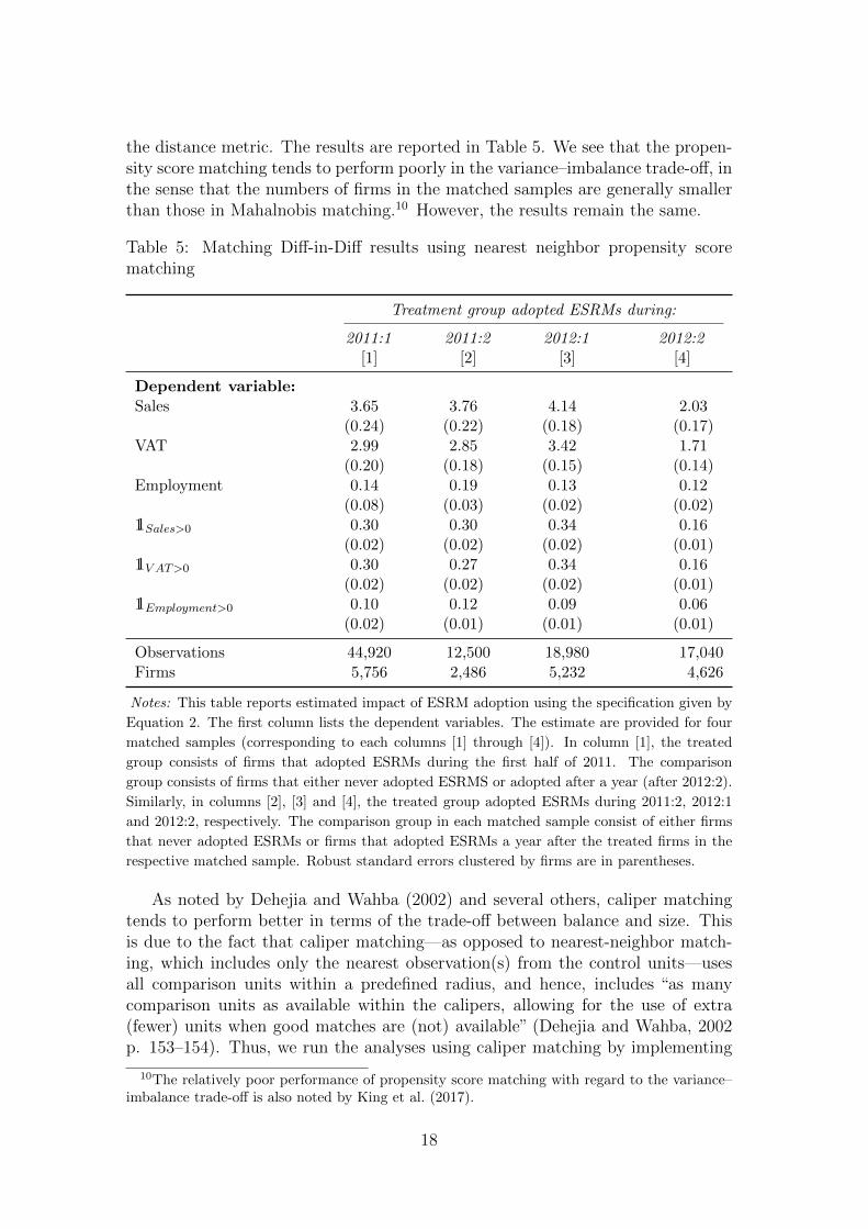
the distance metric. The results are reported in Table 5. We see that the propen-sity score matching tends to perform poorly in the variance–imbalance trade-off, inthe sense that the numbers of firms in the matched samples are generally smallerthan those in Mahalnobis matching.10 However, the results remain the same.
Table 5: Matching Diff-in-Diff results using nearest neighbor propensity scorematching
Treatment group adopted ESRMs during:
2011:1 2011:2 2012:1 2012:2[1] [2] [3] [4]
Dependent variable:Sales 3.65 3.76 4.14 2.03
(0.24) (0.22) (0.18) (0.17)VAT 2.99 2.85 3.42 1.71
(0.20) (0.18) (0.15) (0.14)Employment 0.14 0.19 0.13 0.12
(0.08) (0.03) (0.02) (0.02)11Sales>0 0.30 0.30 0.34 0.16
(0.02) (0.02) (0.02) (0.01)11V AT >0 0.30 0.27 0.34 0.16
(0.02) (0.02) (0.02) (0.01)11Employment>0 0.10 0.12 0.09 0.06
(0.02) (0.01) (0.01) (0.01)
Observations 44,920 12,500 18,980 17,040Firms 5,756 2,486 5,232 4,626
Notes: This table reports estimated impact of ESRM adoption using the specification given by
Equation 2. The first column lists the dependent variables. The estimate are provided for four
matched samples (corresponding to each columns [1] through [4]). In column [1], the treated
group consists of firms that adopted ESRMs during the first half of 2011. The comparison
group consists of firms that either never adopted ESRMS or adopted after a year (after 2012:2).
Similarly, in columns [2], [3] and [4], the treated group adopted ESRMs during 2011:2, 2012:1
and 2012:2, respectively. The comparison group in each matched sample consist of either firms
that never adopted ESRMs or firms that adopted ESRMs a year after the treated firms in the
respective matched sample. Robust standard errors clustered by firms are in parentheses.
As noted by Dehejia and Wahba (2002) and several others, caliper matchingtends to perform better in terms of the trade-off between balance and size. Thisis due to the fact that caliper matching—as opposed to nearest-neighbor match-ing, which includes only the nearest observation(s) from the control units—usesall comparison units within a predefined radius, and hence, includes “as manycomparison units as available within the calipers, allowing for the use of extra(fewer) units when good matches are (not) available” (Dehejia and Wahba, 2002p. 153–154). Thus, we run the analyses using caliper matching by implementing
10The relatively poor performance of propensity score matching with regard to the variance–imbalance trade-off is also noted by King et al. (2017).
18

the algorithm that Lechner et al. (2011) proposed.11 The results are reported inTable 6. We see that the results remain similar.
Table 6: Matching Diff-in-Diff results using radius matching
Treatment group adopted ESRMs during:
2011:1 2011:2 2012:1 2012:2
[1] [2] [3] [4]
Dependent variable:Sales 3.93 3.86 4.56 2.64
(0.22) (0.23) (0.16) (0.14)VAT 3.21 3.11 3.79 2.12
(0.19) (0.19) (0.14) (0.12)Employment 0.23 0.25 0.14 0.12
(0.03) (0.04) (0.02) (0.02)11Sales>0 0.31 0.31 0.37 0.20
(0.02) (0.02) (0.01) (0.01)11V AT >0Post 0.30 0.30 0.37 0.19
(0.02) (0.02) (0.01) (0.01)11Employment>0Post 0.11 0.14 0.09 0.07
(0.01) (0.02) (0.01) (0.01)
Observations 106,910 72,925 107,560 119,175Firms 22,943 15,806 23,780 25,679
Notes: This table reports estimated impact of ESRM adoption using the specification given by
Equation 2. The first column lists the dependent variables. The estimate are provided for four
matched samples (corresponding to each columns [1] through [4]). In column [1], the treated
group consists of firms that adopted ESRMs during the first half of 2011. The comparison
group consists of firms that either never adopted ESRMS or adopted after a year (after 2012:2).
Similarly, in columns [2], [3] and [4], the treated group adopted ESRMs during 2011:2, 2012:1
and 2012:2, respectively. The comparison group in each matched sample consist of either firms
that never adopted ESRMs or firms that adopted ESRMs a year after the treated firms in the
respective matched sample. Robust standard errors clustered by firms are in parentheses.
We have also checked robustness of the results to adjusting the balancing cri-teria by which we prune the sample. Instead of using 5% as a cutoff MSB valueto prune observations, we used 3% and 10% as cutoff MSB values. These changesare not found to alter the results—reported sales, VAT payments, and employmentshow a significant increase following ESRM adoption.
11The caliper-matching algorithm developed by Lechner et al. (2011) involves four majorsteps. First, probability of treatment (propensity score) is estimated using a standard probitmodel. Second, for each treatment unit, Mahalanobis distances between the treatment unitand comparison units are computed (over a subset of the matching covariates and the estimatedpropensity scores). Third, each treatment unit is matched with a set of comparison units that liewithin a given distance (or radius) from the treatment unit. Finally, control units are weighted,based on their similarity (as defined by the Mahalanobis distance) with the treatment units withwhich they are matched.
19
Our next sets of robustness checks relate to the external effects, which mayarise if the adoption of ESRMs by some firms affects outcomes for non-adopters.Such external effects may occur particularly among firms within the same localityor sector. For example, if ESRM adopters become more competitive (vis-a-visnon-adopters), non-adopters may lose some of their market shares; hence, sales,VAT payments, and employment by non-adopters may decrease. In this this case,the observed difference between adopters and non-adopters is due to not onlyincreases by adopters, but also decreases by non-adopters. Hence, coefficientsfrom the matching regressions may over-estimate the effect. On the contrary,the coefficients could under-estimate the effect if ESRM adopters become lesscompetitive and lose some of their market share.
In order to address this concern, we reran the analysis, after excluding (fromthe comparison group) observations located in districts with relatively high levelsof adoption rates. The assumption is that external effects are likely to matter inareas with high adoption rates. Hence, if the results are driven by external effects,they should not hold when the comparison group includes only the observationsthat are located in districts with low adoption rates (as they are unlikely to havebeen affected by the externalities). We first ranked districts according to theshare of firms that adopted ESRMs in each district (as of the period in which thetreatment firms adopted ESRMs). We then dropped all untreated observationslocated in districts where the adoption rate is above the median district and reranthe analysis. Table 7 reports the results. The matched sample size is now smalleras we have fewer firms to match. However, the results remain the same.
One may, perhaps, be concerned that the external effects could work throughsectors rather than locations. Thus, we also ranked sectors according to rate ofESRM adoption (i.e., the fraction of firms in the sector that adopted ESRMs). Wethen reran the analysis after excluding observations (from the comparison group)where the adoption rate for the firm’s sector is above that of the median sector.We found similar results.
Finally, we have undertaken placebo analyses to assess whether the differencebetween the treated and comparison groups would occur in periods that are pre-sumably unaffected by ESRM adoption. Recall that in the previously describedmatching analysis, we included—among others—the first and second lags of theoutcome variables in the matching covariates. Thus, the matching analysis in-volved selecting treated and comparison firms based on their similarity during thematching periods (i.e., the two periods preceding ESRM adoption), and then com-paring trend differences between the groups during the postmatching periods. Theassumption is that, in absence of the treatment, the treated and comparison groupswould have displayed similar trends outside the matching period. One would thenexpect the two groups to display similar trends during the prematching periods(as opposed to the postmatching periods), since ESRMs had not yet taken effect.The presence of significant differences during the prematching periods would castdoubt on the assumption that, in the absence of ESRM adoption, the two groupswould have similar trends outside the matching periods.
Panel (A) of Figure (3) presents the trend differences in sales during the match-
20

Table 7: Accounting for external effects: Results from Matching Diff-in-Diff whencomparison units are drown from districts with low adoption rates
Treatment group adopted ESRMs during:
2011:1 2011:2 2012:1 2012:2
[1] [2] [3] [4]
Dependent variable:Sales 3.68 3.00 3.29 1.91
(0.38) (0.27) (0.21) (0.20)VAT 3.02 2.14 2.83 1.63
(0.32) (0.22) (0.18) (0.17)Employment 0.34 0.33 0.16 0.08
(0.02) (0.03) (0.01) (0.02)11Sales>0 0.30 0.24 0.27 0.15
(0.03) (0.02) (0.02) (0.02)11V AT >0 0.29 0.21 0.27 0.15
(0.03) (0.02) (0.02) (0.02)11Employment>0 0.16 0.18 0.10 0.04
(0.01) (0.01) (0.01) (0.01)
Observations 51,680 17,070 31,220 18,780Firms 11,736 4,868 6,718 5,082
Notes: This table reports estimated impact of ESRM adoption using the specification given by
Equation 2. The first column lists the dependent variables. The estimate are provided for four
matched samples (corresponding to each columns [1] through [4]). In column [1], the treated
group consists of firms that adopted ESRMs during the first half of 2011. The comparison
group consists of firms that either never adopted ESRMS or adopted after a year (after 2012:2).
Similarly, in columns [2], [3] and [4], the treated group adopted ESRMs during 2011:2, 2012:1
and 2012:2, respectively. The comparison group in each matched sample consist of either firms
that never adopted ESRMs or firms that adopted ESRMs a year after the treated firms in the
respective matched sample. Robust standard errors clustered by firms are in parentheses.
21

ing and postmatching periods, that is, it visually displays the impact of ESRMadoption estimated from the matching diff-in-diff specification (see Table 4). Panel(B) shows the placebo comparison where we plot trend differences during thematching and prematching periods. Each row represents one of the four matchedsamples. Whereas the first column shows the trends as we move from the matchingperiod towards the postmatching period, the second column displays the trends aswe move (back in time) from the matching period towards the prematching period.The vertical lines in the first column represent the actual treatment period (begin-ning of postmatching period), while the vertical lines in the second column showthe placebo period (beginning of prematching period). The vertical axes withineach row have the same scale so that displayed differences between the placeboand treatment effects are directly comparable.
These figures show that the increase in reported sales occurs only when wemove from the matching period to the postmatching period. The changes, aswe move from the matching period to the prematching periods (back in time),are relatively small and statistically insignificant, providing no indication thatthe treated comparison groups would diverge in the absence of ESRM adoption.We have done similar comparisons for VAT payments and employment, findingsimilar results—that significant differences arise only in the postmatching period(see Figure .4 and Figure .5 in the Appendix).
5 ESRMs and net entry
As discussed in Section 3, the potential contribution of ESRMs to build fiscalcapacity may be undermined if firms lower their output in response to increases inthe cost of production (due to extra tax liability), thereby leading to erosion of thetax base. Although the positive effect of ESRMs on employment suggests that thismay not be the case, ESRMs may still affect the tax base if they affect the decisionof firms to enter to (or exit from) the formal sector. For example, if ESRMs makeit more difficult for firms to evade taxes, existing firms may respond by leavingthe formal sector and operating informally where they can shun the adoption ofESRMs. Similarly, the threat of ESRM adoption may discourage potential newentrants into the formal sector.
Admittedly, identifying the causal effect of ESRM adoption on net entry (entryminus exit) is difficult. We nonetheless present the available preliminary evidenceon the association between ESRM adoption and net entry. We consider the fol-lowing regression:
NetEntryd,t = ψ × AdoptionRated,t−1 + γt + ωd + εd,t
The outcome variable is the rate of net entry in district d, period t. The rate ofnet entry is defined as the number of newly entered firms minus those that exited(as a share of the total number of exiting firms). AdoptionRated,t−1 is the shareof firms who adopted ESRMs in district d as of period t − 1. γt and ωn are timeand district fixed effects. ψ is the coefficient of interest. A negative value of ψ
22

Figure 3: Trend differences of mean log sales during the matching, postmatchingand prematching periods.
Panel (A): Treatment effect—trend dur-ing matching and post matching period
Panel (B): Placebo effect—trend duringmatching and prematching period
-10
12
34
520
10:1
2010
:2
2011
:1
2011
:2
2012
:1
-10
12
34
2010
:2
2010
:1
2009
:2
2009
:1
2008
:2
-10
12
34
520
10:2
2011
:1
2011
:2
2012
:1
2012
:2
-10
12
34
2011
:1
2010
:2
2010
:1
2009
:2
2009
:1
-10
12
34
520
11:1
2011
:2
2012
:1
2011
:2
2012
:2
-10
12
34
520
11:2
2011
:1
2010
:2
2010
:1
2008
:2
-10
12
320
11:2
2012
:1
2012
:2
2013
:1
2013
:2
-10
12
320
12:1
2011
:2
2011
:1
2010
:2
2010
:1
Notes: The figures show the differences in reported sales between treated and comparison groupsfor four matched samples (corresponding to each row). The vertical lines show the period ofESRM adoption for the treated group.
23

would suggest that districts with aggressive expansions of ESRMs are associatedwith lower rates of net entry.
Table 8: Net entry and the rate of ESRM adoption
Dependent variable:
NetEntryd,t NetEntrys,t
[1] [2] [3] [4]
Right-hand-side variable:
AdoptionRated,t−1 −0.09(0.07)
AdoptionRated,t−2 0.02(0.08)
AdoptionRates,t−1 −0.07(0.07)
AdoptionRates,t−2 −0.06(0.04)
Observations 2,491 2,429 2,259 2,235Districts (or sectors) 245 242 197 197
Notes: Columns [1] and [2] show the correlations between the current rate of net entry into a
district (NetEntryd,t) and the lags of ESRM adoption rate in the district (AdoptionRated,t−1
and AdoptionRated,t−2). Columns [3] and [4] show show the correlation between the current
rate of net entry into sectors s (NetEntrys,t) and the lags of ESRM adoption rate in the sec-
tor (AdoptionRates,t−1 and AdoptionRates,t−2). Robust standard errors clustered by district
(columns [1] and [2]) or sectors (columns [3] and [4]) are in parentheses.
The first column of Table 8 reports the estimate for ψ. There is no significantrelationship between rate of ESRM adoption and net entry rate. In the secondcolumn, we include the second lag of ESRM adoption rate within the district(AdoptionRated,t−2) as the right-hand side variable. The result remains the same.In the third and fourth columns, we look at the correlation between the rate ofnet entry into a sector (NetEntrys,t) and the lags of ESRM adoption rate by firmswithin that sector (AdoptionRates,t−1 in the third column and AdoptionRates,t−2in the fourth column). These results also show no significant association betweenthe rate of ESRM adoption and net entry across sectors.
6 Conclusion
Limited fiscal capacity of states has received increased attention as an importantconstraint to economic development. Having an effective tax system requires avast administrative infrastructure capable of gathering, analyzing, and monitor-ing earnings information of a large number of taxpayers—a capacity that manydeveloping countries tend to lack. Thus, the advent of electronic systems has at-tracted governments in many developing countries as a relatively cheap alternative
24
for monitoring earnings information and improving fiscal capacity. In this study,using data from Ethiopia, we document the first empirical evidence on one suchpolicy experiments.
We find that tax payments by firms increase in the aftermath of the ESRMadoption. We also find that the increased tax payments by registered taxpayersdo not appear to have led to erosion of the tax base. By and large, these empiricalpatterns point to a possible positive contribution of the IT revolution to fiscalcapacity in developing countries.
References
Acemoglu, Daron, “Politics and economics in weak and strong states,” Journalof Monetary Economics, October 2005, 52 (7), 1199–1226.
Akcigit, Ufuk, Harun Alp, and Michael Peters, “Lack of Selection andLimits to Delegation: Firm Dynamics in Developing Countries,” Working Paper21905, National Bureau of Economic Research January 2016.
Baskaran, Thushyanthan and Arne Bigsten, “Fiscal Capacity and the Qual-ity of Government in Sub-Saharan Africa,” World Development, 2013, 45 (C),92–107.
Becerril, Javier and Awudu Abdulai, “The Impact of Improved Maize Va-rieties on Poverty in Mexico: A Propensity Score-Matching Approach,” WorldDevelopment, 2010, 38 (7), 1024 – 1035.
Besley, Timothy and Torsten Persson, “State Capacity, Conflict, and Devel-opment,” Econometrica, 2010, 78 (1), 1–34.
and , Pillars of Prosperity: The Political Economics of Development Clus-ters, Princeton University Press, 2011.
Best, Michael, Anne Brockmeyer, Henrik Kleven, and Johannes Spin-newijn, “Production vs Revenue Efficiency With Limited Tax Capacity: Theoryand Evidence From Pakistan,” Journal of Political Economy, 2015, (forthcom-ing).
Bird, R. M., “The Administrative Dimension of Tax Reform in Developing Coun-tries,” in Malcolm Gillis, ed., Lessons from Tax Reform in Developing Countries,Duke University Press Durham 1989, pp. 315–46.
Bird, Richard M. and Eric M. Zolt, “Technology and Taxation in DevelopingCountries: From Hand to Mouse,” National Tax Journal, December 2008, 61(4), 791–821.
Blundell, Richard and Monica Costa Dias, “Evaluation Methods for Non-Experimental Data,” Fiscal Studies, 2000, 21 (4), 427–468.
25

Boadway, Robin and Motohiro Sato, “Optimal Tax Design and Enforcementwith an Informal Sector,” American Economic Journal: Economic Policy, 2009,1 (1), 1–27.
Bresnahan, Timothy F., Erik Brynjolfsson, and Lorin M. Hitt, “Informa-tion Technology, Workplace Organization, and the Demand for Skilled Labor:Firm-Level Evidence,” The Quarterly Journal of Economics, 2002, 117 (1), pp.339–376.
Brynjolfsson, Erik and Lorin M. Hitt, “Beyond Computation: InformationTechnology, Organizational Transformation and Business Performance,” TheJournal of Economic Perspectives, 2000, 14 (4), pp. 23–48.
Caliendo, Marco and Sabine Kopeinig, “SOME PRACTICAL GUIDANCEFOR THE IMPLEMENTATION OF PROPENSITY SCORE MATCHING,”Journal of Economic Surveys, 2008, 22 (1), 31–72.
Carrillo, Pau, Dina Pomeranz, and Monica Singha, “Dodging the Taxman:Firm Misreporting and Limits to Tax Enforcement,” Technical Report 15-026,Harvard Business School Working Paper 2014.
Dehejia, Rajeev H. and Sadek Wahba, “Propensity Score-Matching MethodsFor Nonexperimental Causal Studies,” The Review of Economics and Statistics,February 2002, 84 (1), 151–161.
Engel, Eduardo M. R. A., Alexander Galetovic, and Claudio E. Rad-datz, “A Note on Enforcement Spending and VAT Revenues,” Review of Eco-nomics and Statistics, 2001, 83 (2).
Fisman, Raymond and Shang-Jin Wei, “Tax Rates and Tax Evasion: Evi-dence from “Missing Imports” in China,” Journal of Political Economy, 2004,112 (2), pp. 471–496.
Garicano, Luis and Paul Heaton, “Information Technology, Organization, andProductivity in the Public Sector: Evidence from Police Departments,” Journalof Labor Economics, 2010, 28 (1), pp. 167–201.
Girma, Sourafel and Holger Gorg, “Evaluating the foreign ownership wagepremium using a difference-in-differences matching approach,” Journal of Inter-national Economics, May 2007, 72 (1), 97–112.
Gordon, Roger and Wei Li, “Tax structures in developing countries: Manypuzzles and a possible explanation,” Journal of Public Economics, 2009, 93 (7-8), 855 – 866.
Hsieh, Chang-Tai and Benjamin A. Olken, “The Missing "MissingMiddle",” Journal of Economic Perspectives, Summer 2014, 28 (3), 89–108.
26

Imbens, Guido W., “Matching Methods in Practice: Three Examples,” Journalof Human Resources, 2015, 50 (2), 373–419.
Jenkins, Glenn P. and Chun-Yan Kuo, “A VAT Revenue Simulation Modelfor Tax Reform in Developing Countries,” World Development, April 2000, 28(4), 763–774.
Keen, Michael and Jack Mintz, “The optimal threshold for a value-added tax,”Journal of Public Economics, March 2004, 88 (3-4), 559–576.
King, Gary, Christopher Lucas, and Richard A. Nielsen, “The Balance-Sample Size Frontier in Matching Methods for Causal Inference,” AmericanJournal of Political Science, 2017, 61 (2), 473–489.
Kleven, Henrik J. and Mazhar Waseem, “Using Notches to Uncover Opti-mization Frictions and Structural Elasticities: Theory and Evidence from Pak-istan,” The Quarterly Journal of Economics, 2013, 128 (2), 669–723.
Kumler, Todd, Eric Verhoogen, and Judith A. Frıas, “Enlisting Employeesin Improving Payroll-Tax Compliance: Evidence from Mexico,” Working Paper19385, National Bureau of Economic Research August 2013.
Lechner, Michael, Ruth Miquel, and Conny Wunsch, “LONG-RUN EF-FECTS OF PUBLIC SECTOR SPONSORED TRAINING IN WEST GER-MANY,” Journal of the European Economic Association, 2011, 9 (4), 742–784.
Lewis-Faupel, Sean, Yusuf Neggers, Benjamin A. Olken, and RohiniPande, “Can Electronic Procurement Improve Infrastructure Provision? Evi-dence from Public Works in India and Indonesia,” American Economic Journal:Economic Policy, August 2016, 8 (3), 258–83.
Muralidharan, Karthik, Paul Niehaus, and Sandip Sukhtankar, “Build-ing State Capacity: Evidence from Biometric Smartcards in India,” AmericanEconomic Review, October 2016, 106 (10), 2895–2929.
Naritomi, Joana, “Consumers as tax auditors,” 2016.
Olken, Benjamin A. and Monica Singhal, “Informal Taxation,” AmericanEconomic Journal: Applied Economics, October 2011, 3 (4), 1–28.
Pomeranz, Dina, “No Taxation without Information: Deterrence and Self-Enforcement in the Value Added Tax,” American Economic Review, 2015, 105(8), 2539–69.
Rosenbaum, Paul R. and Donald B. Rubin, “The Central Role of the Propen-sity Score in Observational Studies for Causal Effects,” Biometrika, 1983, 70 (1),41–55.
and , “Constructing a Control Group Using Multivariate Matched SamplingMethods That Incorporate the Propensity Score,” The American Statistician,1985, 39 (1), 33–38.
27

Slemrod, Joel, “Does It Matter Who Writes the Check to the Government?The Economics of Tax Remittance,” National Tax Journal, June 2008, 61 (2),251–75.
, Brett Collins, Jeffrey L. Hoopes, Daniel Reck, and Michael Se-bastiani, “Does credit-card information reporting improve small-business taxcompliance?,” Journal of Public Economics, 2017, 149, 1 – 19.
Smith, Jeffrey A. and Petra E. Todd, “Does matching overcome LaLonde’scritique of nonexperimental estimators?,” Journal of Econometrics, 2005, 125(1-2), 305 – 353. Experimental and non-experimental evaluation of economicpolicy and models.
Stiroh, Kevin J., “Information Technology and the U.S. Productivity Revival:What Do the Industry Data Say?,” The American Economic Review, 2002, 92(5), pp. 1559–1576.
Tanzi, Vito and Howell H. Zee, “Tax Policy for Emerging Markets: DevelopingCountries,” National Tax Journal, 2000, 53 (n. 2), 299–322.
28

Appendix
29

Figure .4: Trend differences in mean log VAT during the matching, postmatchingand prematching periods.
Panel (A): Treatment effect—trend dur-ing matching and post matching period
Panel (B): Placebo effect—trend duringmatching and prematching period
-10
12
34
2010
:1
2010
:2
2011
:1
2011
:2
2012
:1
-10
12
34
2010
:2
2010
:1
2009
:2
2009
:1
2008
:2
-10
12
34
2010
:2
2011
:1
2011
:2
2012
:1
2012
:2
-10
12
34
2011
:1
2010
:2
2010
:1
2009
:2
2009
:1
-10
12
34
520
11:1
2011
:2
2012
:1
2011
:2
2012
:2
-10
12
34
520
11:2
2011
:1
2010
:2
2010
:1
2008
:2
-10
12
320
11:2
2012
:1
2012
:2
2013
:1
2013
:2
-10
12
320
12:1
2011
:2
2011
:1
2010
:2
2010
:1
Notes: The figures show the differences in VAT between treated and comparison groups for fourmatched samples (corresponding to each row). The vertical lines show the period of ESRMadoption for the treated group.
30

Figure .5: Trend differences in log employment during the matching, postmatchingand prematching periods.
Panel (A): Treatment effect—trend dur-ing matching and post matching period
Panel (B): Placebo effect—trend duringmatching and prematching period
-.20
.2.4
2010
:1
2010
:2
2011
:1
2011
:2
2012
:1
-.20
.2.4
2010
:2
2010
:1
2009
:2
2009
:1
2008
:2
-.20
.2.4
2010
:2
2011
:1
2011
:2
2012
:1
2012
:2
-.20
.2.4
2011
:1
2010
:2
2010
:1
2009
:2
2009
:1
-.10
.1.2
.320
11:1
2011
:2
2012
:1
2011
:2
2012
:2
-.10
.1.2
.320
11:2
2011
:1
2010
:2
2010
:1
2008
:2
-.10
.1.2
.320
11:2
2012
:1
2012
:2
2013
:1
2013
:2
-.10
.1.2
.320
12:1
2011
:2
2011
:1
2010
:2
2010
:1
Notes: The figures show the differences in employment between treated and comparison groupsfor four matched samples (corresponding to each row). The vertical lines show the period ofESRM adoption for the treated group.
31

Table A1: Balance statistics before and after matching—treated firms adoptedESRMs in 2011:1
Variable Un(matched) Treated Control MSB(%) t-value[1] [2] [3] [4] [5] [6]
log(1 + salest−1) U 9.282 3.621 97.6 71.5M 9.217 9.243 −0.5 −0.3
log(1 + salest−2) U 8.636 4.092 75.3 55.3M 8.652 8.676 −0.4 −0.3
salest−1 > 0 U 0.733 0.289 99.1 72.3M 0.727 0.727 0.1 0.1
salest−2 > 0 U 0.683 0.327 76.3 55.8M 0.684 0.683 0.1 0.1
log(1 + empt−1) U 0.023 0.027 −1.1 −0.8M 0.005 0.005 −0.1 −0.1
log(1 + empt−2) U 0.008 0.025 −6.7 −4.4M 0.004 0.006 −0.8 −1.1
empt−1 > 0 U 0.013 0.009 4.2 3.2M 0.003 0.002 0.4 0.5
empt−2 > 0 U 0.004 0.008 −4.9 −3.4M 0.002 0.002 −0.3 −0.3
age U 6.551 7.865 −28.5 −21M 6.489 6.523 −0.7 −0.5
age2 U 65.003 82.177 −21.7 −16M 63.67 63.554 0.1 0.1
Large U 0.926 0.571 89.8 60.4M 0.932 0.932 0 0
Small U 0.063 0.068 −2.2 −1.6M 0.058 0.058 0 0
LimitedLiability U 0.894 0.615 68.6 47M 0.895 0.896 −0.1 −0.1
Retail U 0.492 0.182 69.5 53.2M 0.496 0.494 0.4 0.2
Service U 0.138 0.063 25 19.4M 0.132 0.132 0 0
SectorSalest−1 U 6.412 6.073 27.3 20M 6.408 6.389 1.5 1
DestrictSalest−1 U 7.83 5.328 103.6 81.9M 7.731 7.656 3.1 1.6
Addis Ababa U 0.986 0.543 122.6 78.9M 0.987 0.987 0 0
Notes: This table reports balance statistics before and after matching. Column [2] describes
whether each row represents an unmatched (U) or matched (M) sample. Columns [3] and [4]
report covariate means for treated and control groups, respectively. Mean Standard Biases are
reported in Column [4]. The last column reports t-values for the mean differences between
treated and control groups.
32

Table A2: Balance statistics before and after matching—treated firms adoptedESRMs in 2011:2
Variable Un(matched) Treated Control MSB(%) t-value[1] [2] [3] [4] [5] [6]
log(1 + salest−1) U 8.732 3.327 91.6 44.6M 8.694 8.699 −0.1 0
log(1 + salest−2) U 7.164 3.475 61.6 30.5M 7.201 7.286 −1.4 −0.5
salest−1 > 0 U 0.692 0.258 96.4 47M 0.689 0.689 0 0
salest−2 > 0 U 0.583 0.28 64.2 31.8M 0.586 0.587 −0.3 −0.1
log(1 + empt−1) U 0.027 0.03 −1.1 −0.5M 0.002 0.001 0.1 0.2
log(1 + empt−2) U 0.021 0.029 −2.5 −1.1M 0.001 0.001 0 0
empt−1 > 0 U 0.017 0.011 5.3 2.8M 0.002 0.002 0 0
empt−2 > 0 U 0.01 0.01 −0.1 −0.1M 0 0 0 0
age U 6.663 8.217 −32.2 −15.4M 6.594 6.534 1.2 0.5
age2 U 67.985 90.633 −26.1 −12.3M 66.612 65.631 1.1 0.4
Large U 0.918 0.575 85.9 34.8M 0.919 0.918 0.1 0.1
Small U 0.053 0.066 −5.4 −2.5M 0.053 0.053 0 0
LimitedLiability U 0.799 0.617 41 18.3M 0.801 0.811 −2.4 −1
Retail U 0.418 0.12 71.2 40.4M 0.424 0.424 −0.2 −0.1
Service U 0.174 0.048 40.8 24.7M 0.17 0.17 0 0
SectorSalest−1 U 6.755 6.255 42.1 19.8M 6.747 6.713 2.8 1.1
DestrictSalest−1 U 7.803 5.571 89.7 50.9M 7.734 7.652 3.3 1
Addis Ababa U 0.86 0.531 76.6 32.7M 0.859 0.856 0.7 0.3
Notes: This table reports balance statistics before and after matching. Column [2] describes
whether each row represents an unmatched (U) or matched (M) sample. Columns [3] and [4]
report covariate means for treated and control groups, respectively. Mean Standard Biases are
reported in Column [4]. The last column reports t-values for the mean differences between
treated and control groups.
33
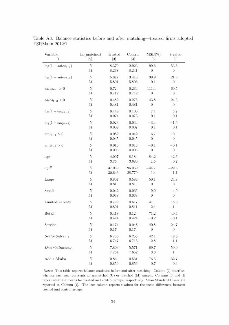
Table A3: Balance statistics before and after matching—treated firms adoptedESRMs in 2012:1
Variable Un(matched) Treated Control MSB(%) t-value[1] [2] [3] [4] [5] [6]
log(1 + salest−1) U 8.379 2.923 99.6 53.6M 8.238 8.241 0 0
log(1 + salest−2) U 5.827 3.446 39.9 21.8M 5.801 5.806 −0.1 0
salest−1 > 0 U 0.72 0.234 111.4 60.5M 0.712 0.712 0 0
salest−2 > 0 U 0.482 0.275 43.8 24.3M 0.481 0.481 0 0
log(1 + empt−1) U 0.149 0.106 7.1 3.7M 0.074 0.073 0.1 0.1
log(1 + empt−2) U 0.023 0.034 −3.4 −1.6M 0.008 0.007 0.1 0.1
empt−1 > 0 U 0.082 0.042 16.7 10M 0.045 0.045 0 0
empt−2 > 0 U 0.013 0.013 −0.1 −0.1M 0.005 0.005 0 0
age U 4.007 8.18 −84.2 −42.6M 3.76 3.686 1.5 0.7
age2 U 37.059 95.059 −44.7 −22.5M 30.643 28.779 1.4 1.1
Large U 0.807 0.583 50.1 24.8M 0.81 0.81 0 0
Small U 0.042 0.065 −9.9 −4.9M 0.038 0.038 0 0
LimitedLiability U 0.799 0.617 41 18.3M 0.801 0.811 −2.4 −1
Retail U 0.418 0.12 71.2 40.4M 0.424 0.424 −0.2 −0.1
Service U 0.174 0.048 40.8 24.7M 0.17 0.17 0 0
SectorSalest−1 U 6.755 6.255 42.1 19.8M 6.747 6.713 2.8 1.1
DestrictSalest−1 U 7.803 5.571 89.7 50.9M 7.734 7.652 3.3 1
Addis Ababa U 0.86 0.531 76.6 32.7M 0.859 0.856 0.7 0.3
Notes: This table reports balance statistics before and after matching. Column [2] describes
whether each row represents an unmatched (U) or matched (M) sample. Columns [3] and [4]
report covariate means for treated and control groups, respectively. Mean Standard Biases are
reported in Column [4]. The last column reports t-values for the mean differences between
treated and control groups.
34

Table A4: Balance statistics before and after matching—treated firms adoptedESRMs in 2012:2
Variable Un(matched) Treated Control MSB(%) t-value[1] [2] [3] [4] [5] [6]
log(1 + salest−1) U 7.628 3.403 69.3 32.6M 7.615 7.633 −0.3 −0.1
log(1 + salest−2) U 5.867 2.998 49.4 23.7M 5.871 5.983 −1.9 −0.6
salest−1 > 0 U 0.603 0.264 72.8 34.3M 0.602 0.603 −0.2 −0.1
salest−2 > 0 U 0.487 0.243 52.3 25.2M 0.487 0.495 −1.6 −0.5
log(1 + empt−1) U 0.397 0.231 17.9 8.6M 0.388 0.376 1.2 0.4
log(1 + empt−2) U 0.316 0.197 13.9 6.6M 0.31 0.303 0.8 0.3
empt−1 > 0 U 0.19 0.091 29 15.1M 0.189 0.188 0.3 0.1
empt−2 > 0 U 0.149 0.079 22.3 11.4M 0.149 0.148 0.3 0.1
age U 5.057 8.037 −55.3 −23.6M 5.031 4.946 1.6 0.6
age2 U 50.571 97.632 −35.5 −13.7M 49.668 47.566 1.6 0.8
Large U 0.577 0.554 4.6 2.1M 0.577 0.571 1.2 0.4
Small U 0.059 0.06 −0.5 −0.2M 0.059 0.058 0.2 0.1
LimitedLiability U 0.788 0.603 41 17.3M 0.787 0.782 1.1 0.4
Retail U 0.273 0.11 42.2 22.4M 0.273 0.268 1.3 0.4
Service U 0.193 0.05 45 27.2M 0.192 0.192 0.1 0
SectorSalest−1 U 7.111 6.143 47.9 21.1M 7.11 7.065 2.2 0.8
DestrictSalest−1 U 6.763 5.565 50 22.1M 6.756 6.68 3.2 1.1
Addis Ababa U 0.371 0.43 −12 −5.3M 0.37 0.361 1.8 0.6
Notes: This table reports balance statistics before and after matching. Column [2] describes
whether each row represents an unmatched (U) or matched (M) sample. Columns [3] and [4]
report covariate means for treated and control groups, respectively. Mean Standard Biases are
reported in Column [4]. The last column reports t-values for the mean differences between
treated and control groups.
35