building and solving large-scale stochastic programs on an affordable distributed computing

Building and Solving Large-scale Stochastic Programs on an

A�ordable Distributed Computing System�

Emmanuel Fragni�erey, Jacek Gondzioz, Jean-Philippe Vial

Logilab, HEC, Section of Management Studies, University of Geneva

102 Bd Carl-Vogt, 1211 Geneva, Switzerland

http://ecolu-info.unige.ch/~logilab/

Logilab Technical Report 1998.11

June 29, 1998, revised February 20, 1999

Abstract

We present an integrated procedure to build and solve big stochastic programming models.

The individual components of the system {the modeling language, the solver and the hardware{

are easily accessible, or a least a�ordable to a large audience. The procedure is applied to a

simple �nancial model, which can be expanded to arbitrarily large sizes by enlarging the number of

scenarios. We generated a model with one million scenarios, whose deterministic equivalent linear

program has 1,111,112 constraints and 2,555,556 variables. We have been able to solve it on the

cluster of ten PCs in less than 3 hours.

Key words. Algebraic modeling language, decomposition methods, distributed systems,

large-scale optimization, stochastic programming.

1 Introduction

Practical implementations of stochastic programming involve two big challenges. First, we have to

build the model: its size is almost invariably large, if not huge, and this task is in itself a challenge for

�This research was supported by the Fonds National de la Recherche Scienti�que Suisse, grants #12-42503.94 and

#1214-049696.96/1.yHEC, Department of Management, University of Lausanne, BFSH1, 1015 Dorigny-Lausanne, Switzerland.zOn leave from the Systems Research Institute, Polish Academy of Sciences, Newelska 6, 01-447 Warsaw, Poland.

1

the user. The second challenge is of course the solving of the models thus generated. In this paper,

we present an integrated procedure to build, and solve stochastic programming models. The model

generation is based on the event tree; it is performed by means of an algebraic modeling language.

The model is then fed to a solver. Computations are distributed on a bundle of PCs.

The procedure is applied to a simple �nancial model, which can be expanded to arbitrarily large

sizes by enlarging the number of scenarios. We have been able to generate a model with one million

scenarios and solve it on the cluster of ten PCs in less than 3 hours. If it had been written as one big

linear program, the model would have involved 1,111,112 constraints and 2,555,556 variables.

Our main purpose in this paper is to show that the challenge of building and solving such big

multistage stochastic programming models could be done by putting together several existing compo-

nents, which individually are easily accessible, or a least a�ordable. The point is that none of these

components is specially tailored or dedicated to stochastic programming. At the one end of the chain,

there is the modeling language. We use GAMS [10], a commercial code, with the SET extension [17]

to transmit information on the block angular structure of the model. In the middle of the chain, we

�nd the solver. It combines ACCPM [25], a general-purpose optimizer for nondi�erentiable optimiza-

tion, and HOPDM [23], an interior point linear programming solver. At the low end of the chain, the

computations are performed on a cluster of PCs, whose monitoring is based on the Beowulf concept

[39] and the MPI libraries [9].

The model we chose to illustrate the procedure is a simple portfolio management involving �ve

decision variables per period and a single budget constraint. There are up to seven stages and ten

random outcomes per period. The model does not include transaction costs. It is well known that

in the absence of transaction costs, myopic policies are su�cient to achieve optimality [27, 28]. The

reason for not including those costs into our model is just the limitation imposed by currently available

algebraic programming languages. Indeed, in the present state of a�airs, it is not possible to generate

the event tree and the associated model through those languages. Developments are in progress [20].

In a preliminary version of this paper [18], we presented an arti�ce that allowed the generation of

the portfolio problem in GAMS. Unfortunately, this arti�ce is not compatible with the presence of

transaction costs. We are convinced that the situation will change in a near future, and that it will be

soon possible to generate more realistic models. We also believe that the model, as it is today, has its

own merits: it is scalable, and it constitutes a genuine computational challenge. The GAMS program

has been fully rewritten [14] to make the model available for benchmarking stochastic programming

optimization codes. We reproduce the simple GAMS program in the appendix.

Our contribution takes place in an area of very active research and implementations. For instance,

2

there exist nowadays specialized stochastic programming tools based on SMPS [5], an extension of

the MPS format, which is speci�cally designed for the generation of multistage stochastic programs.

Alike our procedure, these tools consist in an integrated chain of components, but there are two

major di�erences with our concept. At present, it is extremely di�cult, if not impossible, to connect

those systems with a modeling language. (For an exception, see [11], which designs a link from a

modeling language with SP/OSL [32].) The second point of concern is that the individual components

of the chain are not accessible to the user. In particular, the decomposition algorithm they use is

not substitutable; nor is it possible to distribute computations according to a local design. With

these proviso, those systems {e.g., DECIS [29], MSLiP [19], and SP/OSL [32]{ are quite e�cient, in

particular with respect to memory management and computational time. SP/OSL even o�ers today

a commercial version that functions on parallel systems.

The computational challenge of stochastic programming has been met by many contributions, in

particular by numerous implementations of a parallel cutting plane decomposition. Cutting plane

decomposition was �rst proposed for two-stage stochastic programs by Van Slyke and Wets [37]. Its

multicut variant is attributed to Ruszczynski [36], and Birge and Louveaux [7], while its extension to

multistage stochastic programs is due to Birge [3]. Recent empirical assessments of their computa-

tional performance on various computer systems can be found in [1, 6, 12, 35, 42], not to mention the

numerous studies that apply parallel algorithms based on variable-splitting and augmented Lagrangian

principles, or parallel computations in matrix factorizations in the context of interior point methods

for stochastic programming. The recent surveys [4, 43] review parallel algorithms for stochastic pro-

gramming. Some of these studies were speci�cally adapted to computing systems (e.g. [1, 12, 35]).

Other were developed using the publicly available library PVM for parallel computing and were exe-

cuted on networks of distributed computers; their porting for execution on a network of distributed

Linux PCs would certainly be a straightforward exercise.

The largest stochastic programming problem that has been solved to date seems to be the one

described in [30, 44]: it has 130,172 scenarios and its linear programming representation involves

2,603,440 constraints and 18,224,080 variables. It was solved by an interior point algorithm on a

parallel machine CM-5 with 64 processors.

The paper is organized as follows. In Section 2, we present the formulation of the two stage

stochastic program and its speci�c structure. In Section 3, we explain the main idea behind the

decomposition method and how it applies to the two stage stochastic programming formulation. We

insist on the fact that the cutting planes approach is based on a transformation of the original problem

into a nondi�erentiable one of smaller dimension. The algorithmic procedure that follows is broken

3

into two main components, the master program (query point generator in our terminology) and the

subproblems (oracle). We emphasize that each component is handled by independent solvers. In our

case the master is handled by ACCPM and the subproblems are solved by HOPDM. E�cient restart in

the subproblems is achieved via a warm start procedure [26]. Our presentation allows the description

of alternative decomposition schemes by simple substitution of any of these solvers, in accordance with

the user preferences. In Section 4, we present the complete procedure: it uses the GAMS modeling

language, establishes a link to automatically access the solver and the parallel computation. The

solver is built around two home made products: [23] and [25]. In Section 5, we present experiments

realized with this procedure. Finally, we conclude this paper indicating possible implications of these

developments. In the appendix we present the GAMS program that generates the portfolio model.

2 Multistage stochastic linear programming problems

Stochastic multistage linear programming can be paraphrased as follows.

1. There is an underlying discrete-time state stochastic process over a �nite horizon. The process

can be represented by an event tree. The natural ordering of the tree nodes is compatible with

time (stage) ordering. A scenario is a path from the root of the tree to a leaf.

2. There is a multistage decision process that is compatible with the stochastic process. Namely, at

each stage some decision variables must be �xed based on the sole knowledge of past decisions

and the current node of the event tree.

3. Along a scenario, decision variables must meet a set of linear constraints. The objective is the

weighted sum of values at the terminal (leaf) nodes. The values are themselves linear functions

of the decision variables on the scenario terminating at the leaf node under consideration.

The above de�nition of multistage linear stochastic decision process may be translated into a

linear program. Constraints are formulated along individual scenarios. To this end, we conveniently

introduce decision variables indexed by the scenario. In the original problem, decisions are not taken

with the knowledge of a full scenario, but just from the information at the current node of the event

tree. To meet this requirement we introduce the so-called non-anticipativity constraints. Given a

node, we consider the subpath from the root of the tree to that node. Along that subpath, decision

variables must take the same values for all scenarios sharing the same subpath.

The main issue in practical stochastic linear programming is dimensionality. The discrete stochastic

process is generally an approximation of a continuous process. There is thus a natural tendency to cre-

4

ate very large event trees, and thus many decision variables, linear constraints, and non-anticipativity

constraints.

A considerable reduction in the problem dimension can be achieved by taking a single representative

of the set of decision variables linked by a non-anticipativity constraint. The remark is trivial; however

its implementation through modeling languages is still a challenge. This aspect will be discussed later

in this paper.

After elimination of the non-anticipativity constraints, the straight formulation of the problem

generally results in instances whose size cannot be matched by the current technology (linear pro-

gramming software, available core memory and computing power), at least without resorting to major

modi�cations in the optimization codes. Fortunately enough, these programs are very sparse and

structured. The structure is a consequence of the underlying event tree. To meet the challenge of

multistage stochastic linear programming, we must exploit structure.

2.1 Two stage programs

The two stage version already displays the typical structure of stochastic linear programs. It can be

formulated as follows.

min cTx+PL

j=1 pj(qj)T yj

s.t. Ax = b;

T jx+W jyj = hj; j = 1; : : : ; L;

x � 0; yj; j = 1; 2; : : : ; L;

(1)

where x are �rst stage variables and yj; j = 1; 2; : : : ; L are second stage variables. The constraint

matrix has the so-called dual block angular structure.

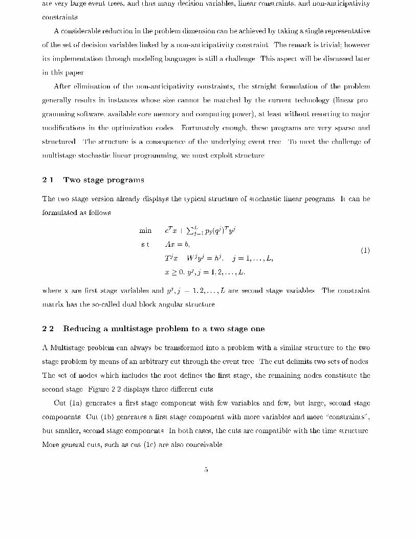
2.2 Reducing a multistage problem to a two stage one

A Multistage problem can always be transformed into a problem with a similar structure to the two

stage problem by means of an arbitrary cut through the event tree. The cut delimits two sets of nodes.

The set of nodes which includes the root de�nes the �rst stage, the remaining nodes constitute the

second stage. Figure 2.2 displays three di�erent cuts.

Cut (1a) generates a �rst stage component with few variables and few, but large, second stage

components. Cut (1b) generates a �rst stage component with more variables and more \constraints",

but smaller, second stage components. In both cases, the cuts are compatible with the time structure.

More general cuts, such as cut (1c) are also conceivable.

5

(a) (b) (c)

Figure 1: Converting a three stage problem into a two-stage problem.

3 Solution methods for two-stage stochastic linear programs

As emphasized before, stochastic multistage linear programs (as well as their formulation as two

stage programs) are naturally very large and possibly huge. The main challenge for the solution

methods are the core memory requirements and the computation time. Those factors are likely to

grow with the problem size at a much faster rate than a linear one. Therefore, users who deal with

multistage stochastic linear programs should either reduce the model size {e.g., by limiting the number

of scenarios by techniques such as importance sampling [29]{, or use solution methods that e�ciently

exploit the special structure of the problem, or distribute computations on independent processors.

These approaches are not exclusive: we should even combine them for improved results. In this paper,

we concentrate on the last two aspects: the algorithmic procedure and parallel computations.

3.1 Algorithmic procedures

Let us discuss the algorithmic procedures �rst.

3.1.1 Direct methods

A direct solution method consists in applying a standard linear programming solver to the global

formulation of the problem. Interior point methods {IPM in short| have the property that the

number of (Newton) iterations necessary to solve the problem is almost insensitive to the problem

size. This property coupled with a clever exploitation of sparse linear algebra enables interior point

6

methods to solve very large scale linear programming problems. Di�culties are known to occur when

the constraint matrix, otherwise sparse, contains dense columns. Since the basic operation in an

IPM iteration consists in forming the product of the scaled constraint matrix by its transpose and

in computing the Cholesky factors of the resulting symmetric matrix, dense columns produce �ll-in

that ruins the approach. Treating dense columns by a Schur complement technique [8] would preserve

sparsity; moreover, the approach parallelizes well [30]. Stochastic linear programs are naturally very

sparse, and have a known sparsity structure, but this structure contains coupling columns (those

associated with the �rst stage variables x). For this reason, standard IPM codes fail to solve large

instances.

3.1.2 Indirect methods

Another approach in the design of e�cient solution methods consists in transforming the initial large

but structured linear program into a convex optimization problem with far fewer variables. In essence

those methods are indirect; their e�ciency strongly depends on the method used to solve the trans-

formed problem. In the case of two stage stochastic linear programs, the transformation is achieved

by Benders decomposition. Although we do not wish to expand on this matter, we would like to

stress that most people refer to Benders decomposition simultaneously as a scheme to transform the

initial problem, and as an algorithm to solve the transformed problem. In the present paper, we use

Benders decomposition to designate the transformation scheme only, and not the algorithm. Benders

decomposition states that Problem (1) can be written in the equivalent form

minfcTx+LX

j=1

Qj(x) j Ax = b; x � 0g; (2)

where Qj(x); j = 1; 2; : : : ; L; is the optimal objective function of the so-called recourse problem

Qj(x) = minfpj(qj)T yj jW jyj = hj � T jx; yj � 0g; (3)

with the understanding that Qj(x) = +1 if Problem (3) is infeasible. The function Qj(x) is convex.

Problem (2) is thus a convex program involving a much smaller number of variables than the original

problem. However, the functions Qj(x) are nondi�erentiable (actually piecewise linear), and the

resolution of problem (2) involves special optimization techniques. Therefore, solving Problem (1) via

Benders decomposition involves the concurrent use of two types of solvers: an LP code to solve the

many problems (3), and a specialized solver for convex nondi�erentiable problems.

Let us point out that the optimal dual solution of Problem 3 has an interesting property. Let uj be

7

the dual solution obtained in solving (3) at x. We can use it to construct the subgradient inequality

Qj(x0) � Qj(x)� (uj)TT j(x0 � x); 8x0: (4)

If Problem (2) is infeasible, its dual is unbounded and for any ray of unboundedness uj , we can

construct the valid inequality

(uj)TT jx0 � (uj)Thj ;8x0: (5)

Finally,

�(x) = cTx+LX

j=1

Qj(x)

is an upper bound for the optimal solution of Problem (1). Note that this upper bound may take the

+1 value if at least one of the problems (3) is infeasible for the current value of x. Any solver for the

convex nondi�erentiable problem (2) makes use of that information, but of that information alone.

Prior to describing a generic method for nondi�erentiable optimization, let us introduce some

useful terminology. Inequalities (4) and (5) de�ne cutting planes. Inequalities (4) are called optimality

cuts, while (5) are called feasibility cuts. We name oracle the process that solves the subproblems (3)

and produces the values for Qj(x), the upper bound �(x) and the cuts (4) or (5). Given a sequence

of query points fxkgk=1;:::K , the answers of the oracle at those points de�ne the following polyhedral

set

LK = f(x; �; z) j Ax = b; x � 0; � =PL

j=1 zj; (6a)

PLj=1 zj � �K ; (6b)

zj � Qj(xk)� (ujk)TT j(x� xk); 8j � L; and 8k such that Qj(x

k) < +1; (6c)

0 � (ujk)Thj � (ujk)TT jx; 8j � L; and 8k such that Qj(xk) = +1g: (6d)

In this expression ujk is either an optimal dual solution for Problem (3) or a ray of unboundedness

of the dual depending on whether Qj(xk) is �nite or not. Also, �K = mink�K �k is the best recorded

upper bound. Clearly LK contains the set of optimal solutions for (1). It is thus named the localization

set.

The solution methods to solve the convex optimization problem (2) cannot use other information

than the cutting planes generated by the oracle at well-chosen query points. This justi�es the generic

name of cutting plane method. We give below a formal statement of a cutting plane method where

some steps are not precisely de�ned to leave room for a variety of implementations. We only assume

that there is an oracle that generates inequalities of type (6c) or (6d) at the successive query points.

8

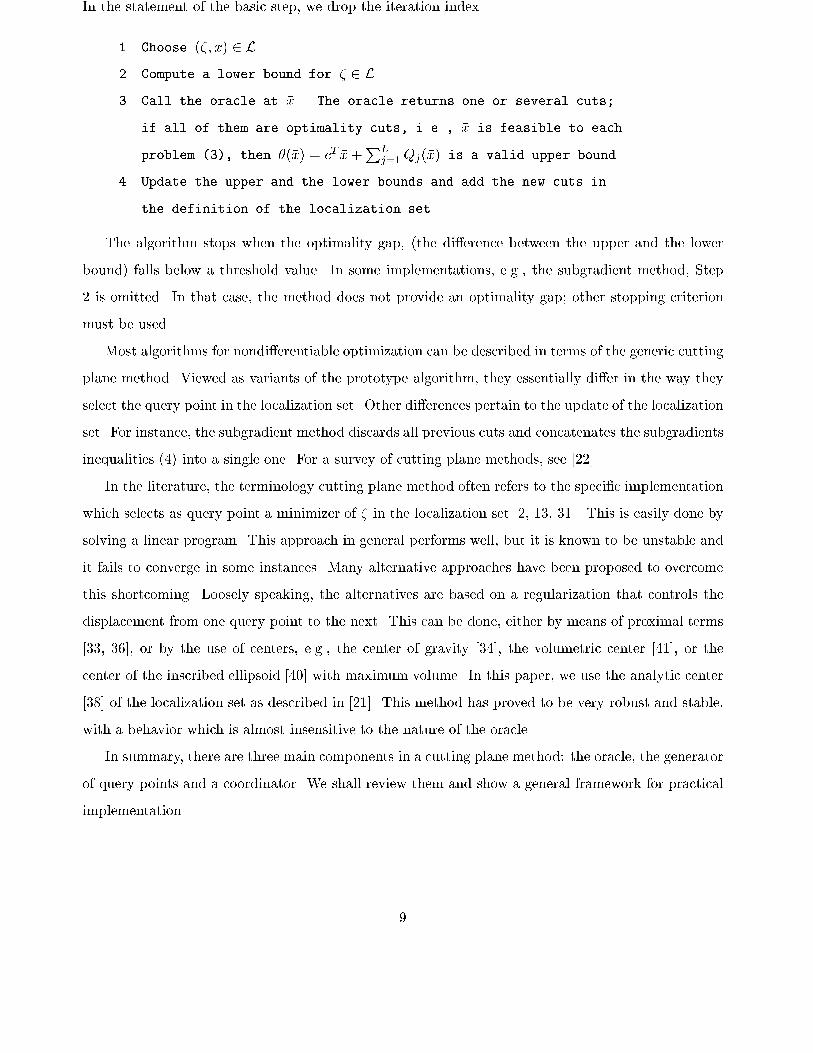
In the statement of the basic step, we drop the iteration index.

1. Choose (��; �x) 2 L.

2. Compute a lower bound for � 2 L.

3. Call the oracle at �x. The oracle returns one or several cuts;

if all of them are optimality cuts, i.e., �x is feasible to each

problem (3), then �(�x) = cT �x+PL

j=1Qj(�x) is a valid upper bound.

4. Update the upper and the lower bounds and add the new cuts in

the definition of the localization set.

The algorithm stops when the optimality gap, (the di�erence between the upper and the lower

bound) falls below a threshold value. In some implementations, e.g., the subgradient method, Step

2 is omitted. In that case, the method does not provide an optimality gap; other stopping criterion

must be used.

Most algorithms for nondi�erentiable optimization can be described in terms of the generic cutting

plane method. Viewed as variants of the prototype algorithm, they essentially di�er in the way they

select the query point in the localization set. Other di�erences pertain to the update of the localization

set. For instance, the subgradient method discards all previous cuts and concatenates the subgradients

inequalities (4) into a single one. For a survey of cutting plane methods, see [22].

In the literature, the terminology cutting plane method often refers to the speci�c implementation

which selects as query point a minimizer of � in the localization set [2, 13, 31]. This is easily done by

solving a linear program. This approach in general performs well, but it is known to be unstable and

it fails to converge in some instances. Many alternative approaches have been proposed to overcome

this shortcoming. Loosely speaking, the alternatives are based on a regularization that controls the

displacement from one query point to the next. This can be done, either by means of proximal terms

[33, 36], or by the use of centers, e.g., the center of gravity [34], the volumetric center [41], or the

center of the inscribed ellipsoid [40] with maximum volume. In this paper, we use the analytic center

[38] of the localization set as described in [21]. This method has proved to be very robust and stable,

with a behavior which is almost insensitive to the nature of the oracle.

In summary, there are three main components in a cutting plane method: the oracle, the generator

of query points and a coordinator. We shall review them and show a general framework for practical

implementation.

9

The coordinator It receives and transmits information between the oracle and the query point

generator. In that respect, it sets the formats in which information is to be exchanged. Its main

function is to update the bounds, and decide upon termination. Additionally, it might keep track of

past generated cutting planes and decide on cut elimination.

The coordinator may also be the place where the �rst stage constraints are handled: they are sent

to the query point generator, once and for all as a set of preliminary cutting planes.

The query point generator The generator stores previously generated cutting planes. It receives

the new cutting planes and the best upper bound. It constructs the current version of the localization

set and generates a query point within it. Some methods only use the most recently generated cutting

planes; they also do not use the upper bound information. We do not discuss it further. Our purpose

is to stress that our framework is general enough to include a large body of methods, not to discuss

them. In some cases, such as the analytic center method, the generator also produces a lower bound.

The oracle The oracle is problem dependent. At the query point x, it computes inequalities of

type (4) or (5) and possibly an upper bound for the optimal solution. In the case of stochastic 2-stage

linear programs, the oracle is made of L independent oracles which consists of solving the subproblems

that are linear programs. If the programs are not too large, we may use the simplex algorithm. In

cases of very large dimensions, we could also use an interior point method. An important issue is the

ability to use the results at the previous query point to perform warm start. This is quite easy with

the simplex algorithm. If the method uses an IPM, it is still possible to use Gondzio's technique [24].

See [26] for a practical implementation. It is also possible to play on the degree of accuracy in solving

the subproblems to enhance solution times of the subproblems. See again [26].

Finally, let us point out that in stochastic multistage linear programs, the subproblems inherit

the basic structure: they could be formulated as 2-stage programs and solved via a cutting plane

technique.

3.2 Parallel computing

To conclude this section, let us brie y discuss the opportunities for distributed computations. Clearly,

the oracle is the candidate of choice for parallel computation in the case of stochastic linear program-

ming. Calls to the oracle are separated by computation of the next query point in the generator. The

latter operation is sequential, unless we go very deep into programming. We do not investigate this

route. To achieve interesting speed-up's when the number of independent processors increases, the

10

model should possess the following characteristics.

1. The query point generator takes far less time than the oracle. This is typically the case when

the �rst stage variable has low dimension, and the subproblems (second stage) are numerous

and/or large.

2. The workload is well-balanced over the various processors. In general, some subproblems take

much more time to be solved than others. If there are as many processors as subproblems,

most processors would experience important waiting times. It is certainly more advantageous to

work with a limited number of processors, each of them treating many subproblems sequentially.

Statistically, the work load will be better balanced.

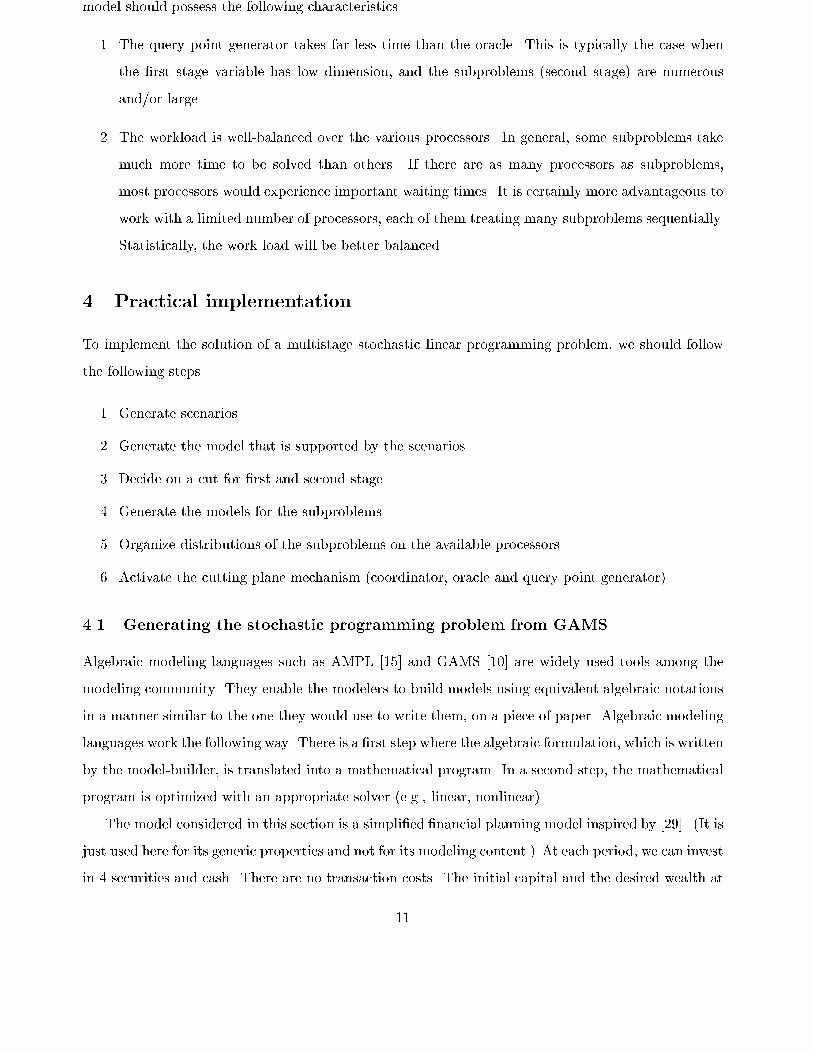
4 Practical implementation

To implement the solution of a multistage stochastic linear programming problem, we should follow

the following steps.

1. Generate scenarios.

2. Generate the model that is supported by the scenarios.

3. Decide on a cut for �rst and second stage.

4. Generate the models for the subproblems.

5. Organize distributions of the subproblems on the available processors.

6. Activate the cutting plane mechanism (coordinator, oracle and query point generator).

4.1 Generating the stochastic programming problem from GAMS

Algebraic modeling languages such as AMPL [15] and GAMS [10] are widely used tools among the

modeling community. They enable the modelers to build models using equivalent algebraic notations

in a manner similar to the one they would use to write them, on a piece of paper. Algebraic modeling

languages work the following way. There is a �rst step where the algebraic formulation, which is written

by the model-builder, is translated into a mathematical program. In a second step, the mathematical

program is optimized with an appropriate solver (e.g., linear, nonlinear).

The model considered in this section is a simpli�ed �nancial planning model inspired by [29]. (It is

just used here for its generic properties and not for its modeling content.) At each period, we can invest

in 4 securities and cash. There are no transaction costs. The initial capital and the desired wealth at

11

the end of the planning period are de�ned exogenously. Prices of securities have been computed by a

multivariate log-normal random generator implemented in MATLAB. Prices are assumed independent

between periods. The time-scale dimension is de�ned over T periods. The uncertainty dimension is

de�ned at each node for N realizations. The corresponding event tree is symmetric and involves N

di�erent branches at each node except for the leaves. Hence the total number of scenarios is NT . The

objective is a piecewise linear function, which corresponds to the expected utility of all scenarios. The

model is written in the GAMS modeling language. The corresponding GAMS model can be found in

the appendix.

Again, we would like to stress that this model is just used to easily generate large problems from

the modeling language. The model has no pretention to be a realistic �nancial model. The main

reason is, simply stated, that without transaction costs, we can, logically, sell all the assets at the

end of each period, and then buy whatever is wanted for the next period. This way, the need to look

ahead when making decisions (the major point in stochastic programming) disappears. Our omission

to include the transaction costs in our formulation comes form a \trick" we are using in GAMS to

produce a stochastic programming structure. With a transaction cost formulation, new variables such

as buy and sell variables have to be included along with new constraints establishing these buy and

sell relations. One way to include them would have been to add locking constraint to ensure that

non-anticipativity constraints are not violated. However, it would have been practically impossible to

do so with very large problems in this environment.

4.2 Invoking SET and BALP from GAMS

A compact formulation written with equivalent algebraic notations along with the data are fed to

the algebraic modeling language. From this point, all operations are automated. The algebraic

modeling language produces the complete mathematical programming formulation. SET [17] provides

the structural information on how to split the anonymous matrix produced by GAMS into blocks

corresponding to the required block-angular formulation. To construct the mapping from the index

sets (e.g., time, scenarios) [16], we require information on

� the number of subproblems;

� the set of rows and columns for each subproblem expressed in terms of the modeling language.

Subproblems are then dispatched to the di�erent PCs.

BALP is an interior point decomposition code [26] that calls for two independent solvers, ACCPM

to compute the analytic center of the localization set and HOPDM to compute optimal solutions for

12

the subproblems. It is implemented on a cluster of 10 Pentium Pro PCs [39] linked with Ethernet

that allows a 10MB/s transfer rate. The operating system is LINUX and the parallel communication

is done with MPI [9].

5 Experiments

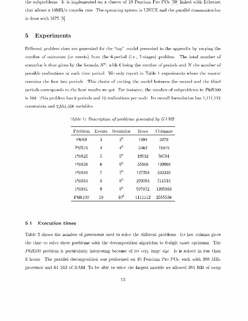
Di�erent problem sizes are generated for the \toy" model presented in the appendix by varying the

number of outcomes (or events) from the 6-period (i.e., 7-stages) problem. The total number of

scenarios is thus given by the formula N6, with 6 being the number of periods and N the number of

possible realizations at each time period. We only report in Table 1 experiments where the master

contains the �rst two periods. This choice of cutting the model between the second and the third

periods corresponds to the best results we got. For instance, the number of subproblems in P6R100

is 100. This problem has 6 periods and 10 realizations per node. Its overall formulation has 1,111,112

constraints and 2,555,556 variables.

Table 1: Description of problems generated by GAMS.

Problem Events Scenarios Rows Columns

P6R9 3 36 1094 3279

P6R16 4 46 5462 15018

P6R25 5 56 19532 50781

P6R36 6 66 55988 139968

P6R49 7 76 137258 333339

P6R64 8 86 299594 711534

P6R81 9 96 597872 1395033

P6R100 10 106 1111112 2555556

5.1 Execution times

Table 2 shows the number of processors used to solve the di�erent problems. Its last column gives

the time to solve these problems with the decomposition algorithm to 6-digit exact optimum. The

P6R100 problem is particularly interesting because of its very large size. It is solved in less than

3 hours. The parallel decomposition was performed on 10 Pentium Pro PCs, each with 200 MHz

processor and 64 MB of RAM. To be able to solve the largest models we allowed 384 MB of swap

13

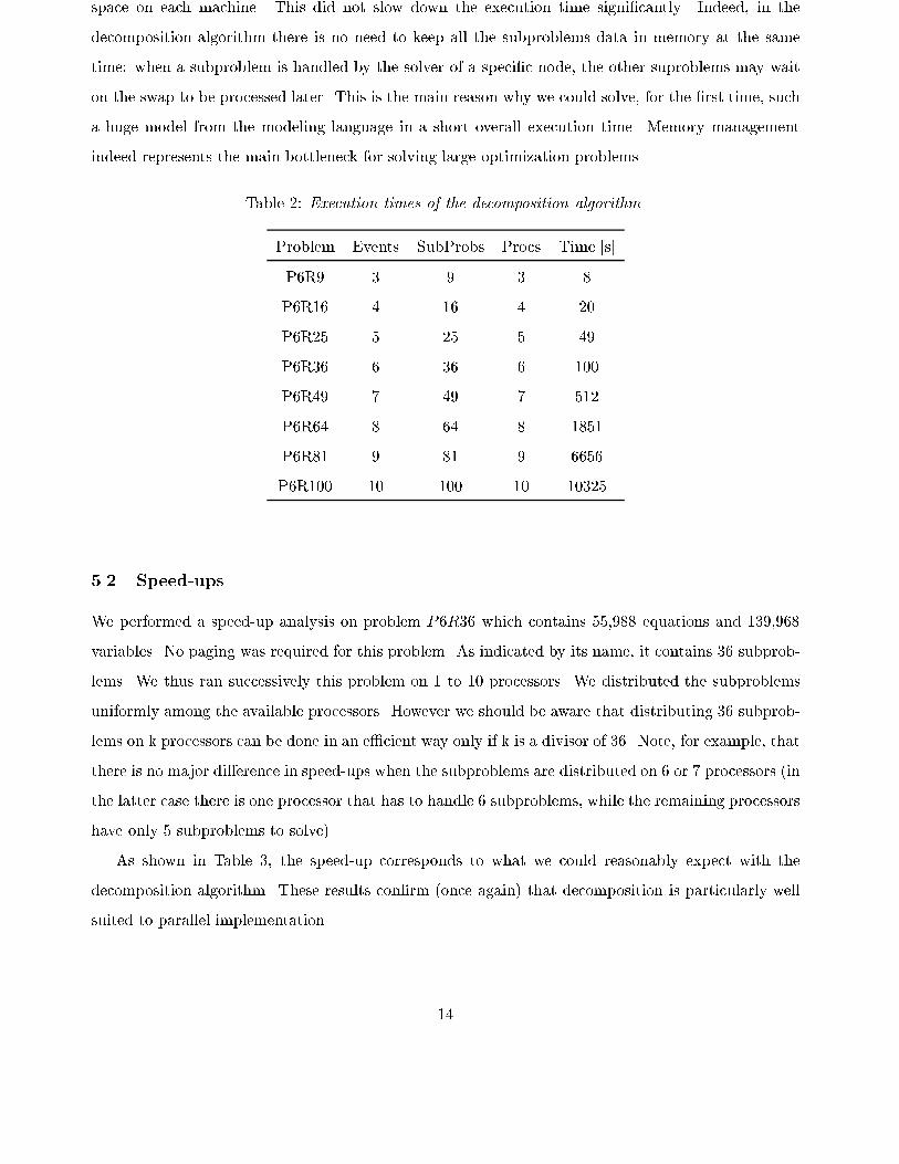
space on each machine. This did not slow down the execution time signi�cantly. Indeed, in the

decomposition algorithm there is no need to keep all the subproblems data in memory at the same

time: when a subproblem is handled by the solver of a speci�c node, the other suproblems may wait

on the swap to be processed later. This is the main reason why we could solve, for the �rst time, such

a huge model from the modeling language in a short overall execution time. Memory management

indeed represents the main bottleneck for solving large optimization problems.

Table 2: Execution times of the decomposition algorithm.

Problem Events SubProbs Procs Time [s]

P6R9 3 9 3 8

P6R16 4 16 4 20

P6R25 5 25 5 49

P6R36 6 36 6 100

P6R49 7 49 7 512

P6R64 8 64 8 1851

P6R81 9 81 9 6656

P6R100 10 100 10 10325

5.2 Speed-ups

We performed a speed-up analysis on problem P6R36 which contains 55,988 equations and 139,968

variables. No paging was required for this problem. As indicated by its name, it contains 36 subprob-

lems. We thus ran successively this problem on 1 to 10 processors. We distributed the subproblems

uniformly among the available processors. However we should be aware that distributing 36 subprob-

lems on k processors can be done in an e�cient way only if k is a divisor of 36. Note, for example, that

there is no major di�erence in speed-ups when the subproblems are distributed on 6 or 7 processors (in

the latter case there is one processor that has to handle 6 subproblems, while the remaining processors

have only 5 subproblems to solve).

As shown in Table 3, the speed-up corresponds to what we could reasonably expect with the

decomposition algorithm. These results con�rm (once again) that decomposition is particularly well

suited to parallel implementation.

14

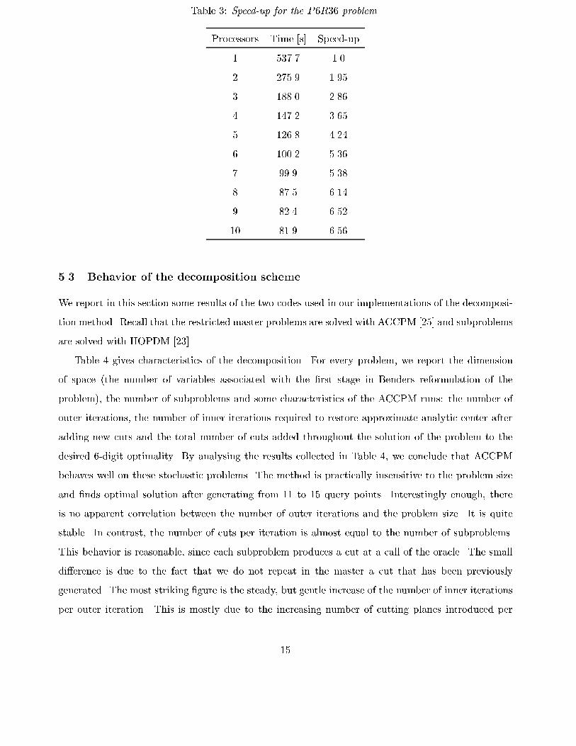
Table 3: Speed-up for the P6R36 problem.

Processors Time [s] Speed-up

1 537.7 1.0

2 275.9 1.95

3 188.0 2.86

4 147.2 3.65

5 126.8 4.24

6 100.2 5.36

7 99.9 5.38

8 87.5 6.14

9 82.4 6.52

10 81.9 6.56

5.3 Behavior of the decomposition scheme

We report in this section some results of the two codes used in our implementations of the decomposi-

tion method. Recall that the restricted master problems are solved with ACCPM [25] and subproblems

are solved with HOPDM [23].

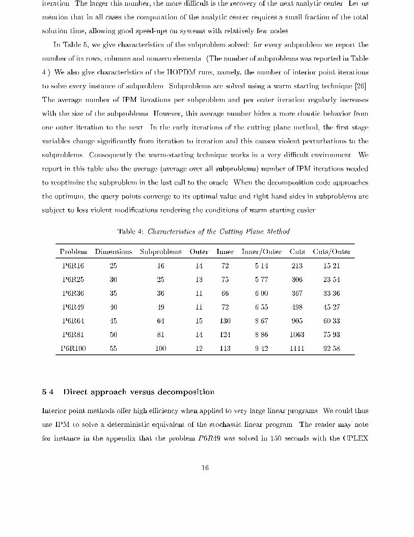
Table 4 gives characteristics of the decomposition. For every problem, we report the dimension

of space (the number of variables associated with the �rst stage in Benders reformulation of the

problem), the number of subproblems and some characteristics of the ACCPM runs: the number of

outer iterations, the number of inner iterations required to restore approximate analytic center after

adding new cuts and the total number of cuts added throughout the solution of the problem to the

desired 6-digit optimality. By analysing the results collected in Table 4, we conclude that ACCPM

behaves well on these stochastic problems. The method is practically insensitive to the problem size

and �nds optimal solution after generating from 11 to 15 query points. Interestingly enough, there

is no apparent correlation between the number of outer iterations and the problem size. It is quite

stable. In contrast, the number of cuts per iteration is almost equal to the number of subproblems.

This behavior is reasonable, since each subproblem produces a cut at a call of the oracle. The small

di�erence is due to the fact that we do not repeat in the master a cut that has been previously

generated. The most striking �gure is the steady, but gentle increase of the number of inner iterations

per outer iteration. This is mostly due to the increasing number of cutting planes introduced per

15

iteration. The larger this number, the more di�cult is the recovery of the next analytic center. Let us

mention that in all cases the computation of the analytic center requires a small fraction of the total

solution time, allowing good speed-ups on systems with relatively few nodes.

In Table 5, we give characteristics of the subproblem solved: for every subproblem we report the

number of its rows, columns and nonzero elements. (The number of subproblems was reported in Table

4.) We also give characteristics of the HOPDM runs, namely, the number of interior point iterations

to solve every instance of subproblem. Subproblems are solved using a warm starting technique [26].

The average number of IPM iterations per subproblem and per outer iteration regularly increases

with the size of the subproblems. However, this average number hides a more chaotic behavior from

one outer iteration to the next. In the early iterations of the cutting plane method, the �rst stage

variables change signi�cantly from iteration to iteration and this causes violent perturbations to the

subproblems. Consequently the warm-starting technique works in a very di�cult environment. We

report in this table also the average (average over all subproblems) number of IPM iterations needed

to reoptimize the subproblem in the last call to the oracle. When the decomposition code approaches

the optimum, the query points converge to its optimal value and right hand sides in subproblems are

subject to less violent modi�cations rendering the conditions of warm starting easier.

Table 4: Characteristics of the Cutting Plane Method

Problem Dimensions Subproblems Outer Inner Inner/Outer Cuts Cuts/Outer

P6R16 25 16 14 72 5.14 213 15.21

P6R25 30 25 13 75 5.77 306 23.54

P6R36 35 36 11 66 6.00 367 33.36

P6R49 40 49 11 72 6.55 498 45.27

P6R64 45 64 15 130 8.67 905 60.33

P6R81 50 81 14 124 8.86 1063 75.93

P6R100 55 100 12 113 9.42 1111 92.58

5.4 Direct approach versus decomposition

Interior point methods o�er high e�ciency when applied to very large linear programs. We could thus

use IPM to solve a deterministic equivalent of the stochastic linear program. The reader may note

for instance in the appendix that the problem P6R49 was solved in 150 seconds with the CPLEX

16

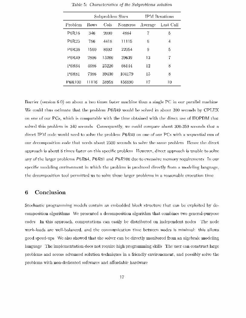
Table 5: Characteristics of the Subproblems solution

Subproblem Sizes IPM Iterations

Problem Rows Cols Nonzeros Average Last Call

P6R16 346 2000 4884 7 5

P6R25 786 4418 11115 6 4

P6R36 1560 8602 22054 9 5

P6R49 2806 15260 39639 13 7

P6R64 4686 25220 66144 12 8

P6R81 7386 39430 104179 15 8

P6R100 11116 58958 156690 17 10

Barrier (version 6.0) on about a two times faster machine than a single PC in our parallel machine.

We could thus estimate that the problem P6R49 would be solved in about 300 seconds by CPLEX

on one of our PCs, which is comparable with the time obtained with the direct use of HOPDM that

solved this problem in 340 seconds. Consequently, we could compare about 300-350 seconds that a

direct IPM code would need to solve the problem P6R49 on one of our PCs with a sequential run of

our decomposition code that needs about 2500 seconds to solve the same problem. Hence the direct

approach is about 8 times faster on this speci�c problem. However, direct approach is unable to solve

any of the larger problems P6R64, P6R81 and P6R100 due to excessive memory requirements. In our

speci�c modeling environment in which the problem is produced directly from a modeling language,

the decomposition tool permitted us to solve these larger problems in a reasonable execution time.

6 Conclusion

Stochastic programming models contain an embedded block structure that can be exploited by de-

composition algorithms. We presented a decomposition algorithm that combines two general-purpose

codes. In this approach, computations can easily be distributed on independent nodes. The node

work-loads are well-balanced, and the communication time between nodes is minimal: this allows

good speed-ups. We also showed that the solver can be directly monitored from an algebraic modeling

language. The implementation does not require high programming skills. The user can construct large

problems and access advanced solution techniques in a friendly environement, and possibly solve the

problems with non-dedicated softwares and a�ordable hardware.

17

Despite its academic character, our test problem is computationally challenging. Our results show

that a problem with over one million constraints and two million variables can be solved in reasonable

time on a cluster of only 10 PCs. This fosters great expectations for solving huge realistic problems

in a near future, using only standard tools and equipment.

An obvious path for future research and implementation is to resort to nested decomposition. As

we pointed it out, the subproblems in the second stage inherit the block structure typical of stochastic

programming. If the subproblems become large, it would be natural to solve them by decomposition.

This would lead to the use of a nested decomposition such as for example [3, 19, 32]

Acknowledgments

The authors gratefully acknowledge the thorough work of the referees and the editor. Their con-

structive criticisms led to a major revision of the paper and made it possible to greatly improve the

presentation.

References

[1] K. A. Ariyawansa and D. D. Hudson, Performance of a benchmark parallel implementation

of the Van Slyke and Wets algorithm for two-stage stochastic programs on the sequent/balance,

Concurrency : Practice and Experience, 3 (1991), pp. 109{128.

[2] J. F. Benders, Partitioning procedures for solving mixed-variables programming problems, Nu-

merische Mathematik, 4 (1962), pp. 238{252.

[3] J. R. Birge, Decomposition and partitioning methods for multistage stochastic linear programs,

Operations Research, 33 (1985), pp. 989{1007.

[4] , Stochastic programming computation and applications, INFORMS Journal on Computing,

9 (1997), pp. 111{133.

[5] J. R. Birge, M. A. H. Dempster, H. I. Gassmann, E. A. Gunn, A. J. King, and S. W.

Wallace, A standard input format for multiperiod stochastic linear programs, Committee on

Algorithms Newsletter, 17 (1988), pp. 1{19.

[6] J. R. Birge, C. J. Donohue, D. F. Holmes, and O. G. Svintsiski, A parallel implementa-

tion of the nested decomposition algorithm for multistage stochastic linear programs, Mathematical

Programming, 75 (1996), pp. 327{352.

18

[7] J. R. Birge and F. V. Louveaux, A multicut algorithm for two-stage stochastic linear pro-

grams, European Journal of Operational Research, 34 (1998), pp. 384{392.

[8] J. R. Birge and L. Qi, Computing block-angular Karmarkar projections with applications to

stochastic programming, Management Science, 34 (1988), pp. 1472{1479.

[9] P. Bridges, N. Doss, W. Gropp, E. Karrels, E. Lusk, and A. Skjellum, User's Guide

to MPICH, a Portable Implementation of MPI, Argonne National Laboratory, September 1995.

[10] A. Brooke, D. Kendrick, and A. Meeraus, GAMS: A User's Guide, The Scienti�c Press,

Redwood City, California, 1992.

[11] C. Condevaux-Lanloy and E. Fragni�ere, Including uncertainty management in energy and

environmental planning, in Proc. of the Fifth International Conference of the Decision Science

Institute (to appear), Athens - Greece, July 4-7 1999.

[12] G. B. Dantzig, J. K. Ho, and G. Infanger, Solving stochastic linear programs on a hypercube

multiprocessor, tech. report, Stanford University, Report SOL-91-10, Department of Operations

Research, January 1991.

[13] G. B. Dantzig and P. Wolfe, The decomposition algorithm for linear programming, Econo-

metrica, 29 (1961), pp. 767{778.

[14] S. Dirkse, Private communication. GAMS Development Corporation, 1998.

[15] R. Fourer, D. Gay, and B. W. Kernighan, AMPL: A Modeling Language for Mathematical

Programming, The Scienti�c Press, San Francisco, California, 1993.

[16] E. Fragni�ere, J. Gondzio, and R. Sarkissian, Customized block structures in algebraic

modeling languages: the stochastic programming case, in Proceedings of the CEFES/IFAC98,

S. Holly, ed., Amsterdam, 1998, Elsevier Science.

[17] E. Fragni�ere, J. Gondzio, R. Sarkissian, and J.-P. Vial, Structure exploiting tool in

algebraic modeling languages, tech. report, Logilab, Section of Management Studies, University

of Geneva, 102 Bd Carl Vogt, CH-1211 Geneva 4, Switzerland, June 1997, revised in June 1998.

[18] E. Fragni�ere, J. Gondzio, and J.-P. Vial, A planning model with one million scenarios

solved on an a�ordable parallel machine, tech. report, Logilab, Section of Management Studies,

University of Geneva, 102 Bd Carl Vogt, CH-1211 Geneva 4, Switzerland, June 1998.

19

[19] H. I. Gassmann, MSLiP: A computer code for the multistage stochastic linear programming

problems, Mathematical Programming, 47 (1990), pp. 407{423.

[20] H. I. Gassmann and A. M. Ireland, Scenario formulation in an algebraic modeling language,

Annals of Operations Research, 59 (1995), pp. 45{75.

[21] J.-L. Goffin, A. Haurie, and J.-P. Vial, Decomposition and nondi�erentiable optimization

with the projective algorithm, Management Science, 38 (1992), pp. 284{302.

[22] J.-L. Goffin and J.-P. Vial, Convex nondi�erentiable optimization: a survey on the analytic

center cutting plane method, tech. report, HEC/Logilab, University of Geneva, 1204 Geneva,

Switzerland, November 1998.

[23] J. Gondzio, HOPDM (version 2.12) { a fast LP solver based on a primal-dual interior point

method, European Journal of Operational Research, 85 (1995), pp. 221{225.

[24] , Warm start of the primal-dual method applied in the cutting plane scheme, Mathematical

Programming, 83 (1998), pp. 125{143.

[25] J. Gondzio, O. du Merle, R. Sarkissian, and J.-P. Vial, ACCPM - a library for convex

optimization based on an analytic center cutting plane method, European Journal of Operational

Research, 94 (1996), pp. 206{211.

[26] J. Gondzio and J.-P. Vial, Warm start and "-subgradients in cutting plane scheme for block-

angular linear programs, tech. report, Logilab, University of Geneva, 102 Bd Carl-Vogt, CH-1211,

June 1997, revised in November 1997. To appear in Computational Optimization and Applications.

[27] N. H. Hakansson, On optimal myopic portfolio policies, with and without serial correlations of

yields, Journal of Business, 44 (1971).

[28] , Convergence to isoelastic utility and policy in multiperiod portfolio choice, Journal of Fi-

nancial Economics, 1 (1974), pp. 201{224.

[29] G. Infanger, Planning under Uncertainty, Boyd and Fraser, Massachusetts, 1994.

[30] E. R. Jessup, D. Yang, and S. A. Zenios, Parallel factorization of structured matrices arising

in stochastic programming, SIAM Journal on Optimization, 4 (1994), pp. 833{846.

[31] J. E. Kelley, The cutting plane method for solving convex programs, Journal of the SIAM, 8

(1960), pp. 703{712.

20

[32] A. J. King, S. E. Wright, and R. Entriken, SP/OSL Version 1.0: Stochastic Programming

Interface Library User's Guide, IBM Research Division,York Heights, 1994.

[33] C. Lemar�echal, A. Nemirovskii, and Y. Nesterov, New variants of bundle methods, Math-

ematical Programming, 69 (1995), pp. 111{147.

[34] A. Levin, An algorithm of minimization of convex functions, Soviet Mathematics Doklady, 160

(1965), pp. 1244{1247.

[35] S. N. Nielsen and S. A. Zenios, Scalable parallel Benders decomposition for stochastic linear

programming, Parallel Computing, 23 (1997), pp. 1069{1088.

[36] A. Ruszczy�nski, A regularized decomposition method for minimizing a sum of polyhedral func-

tions, Mathematical Programming, 33 (1985), pp. 309{333.

[37] R. V. Slyke and R.-B. Wets, L-shaped linear programs with applications to optimal control

and stochastic programming, SIAM Journal of Applied Mathematics, 17 (1969), pp. 638{663.

[38] G. Sonnevend, New algorithms in convex programming based on a notion of "centre" (for sys-

tems of analytic inequalities) and on rational extrapolation, in Trends in Mathematical Optimiza-

tion : Proceedings of the 4th French{German Conference on Optimization in Irsee, Germany,

April 1986, K. H. Ho�mann, J. B. Hiriart-Urruty, C. Lemar�echal, and J. Zowe, eds., vol. 84

of International Series of Numerical Mathematics, Birkh�auser Verlag, Basel, Switzerland, 1988,

pp. 311{327.

[39] T. Sterling, D. J. Becker, D. Savarese, J. E. Dorband, U. A. Ranawake, and C. V.

Packer, Beowulf: A parallel workstation for scienti�c computation. Proceedings, International

Parallel Processing Symposium, 1995.

[40] S. Tarasov, L. Khachiyan, and I. Erlich, The method of inscribed ellipsoids, Soviet Math-

ematics Doklady, 37 (1988).

[41] P. Vaidya, A new algorithm for minimizing convex functions over convex sets, Mathematical

Programming, 73 (1996), pp. 291{341.

[42] H. Vladimiriou, Computational assessment of distributed decomposition methods for stochastic

linear programs, SIAM Journal of Applied Mathematics, 108 (1998), pp. 653{670.

21

[43] H. Vladimiriou and S. A. Zenios, Parallel algorithms for large-scale stochastic programming,

in Parallel Computing in Optimization, S. Migdalas, P. Pardalos, and S. Stor�y, eds., Kluwer

Academic Publishers, 1997, pp. 413{469.

[44] S. A. Zenios, Parallel and supercomputing in the practice of management science, Interfaces, 24

(1994), pp. 122{140.

22

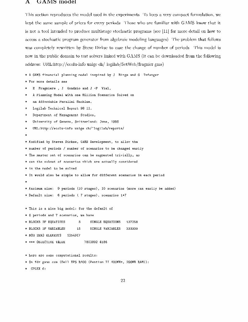
A GAMS model

This section reproduces the model used in the experiments. To keep a very compact formulation, we

kept the same sample of prices for every periods. Those who are familiar with GAMS know that it

is not a tool intended to produce multistage stochastic programs (see [11] for more detail on how to

access a stochastic program generator from algebraic modeling languages). The problem that follows

was completely rewritten by Steve Dirkse to ease the change of number of periods. This model is

now in the public domain to test solvers linked with GAMS (it can be downloaded from the following

address: URL:http://ecolu-info.unige.ch/ logilab/SetWeb/fragnier.gms).

* A GAMS financial planning model inspired by J. Birge and G. Infanger.

* For more details see

* E. Fragniere , J. Gondzio and J.-P. Vial,

* A Planning Model with one Million Scenarios Solved on

* an Affordable Parallel Machine,

* Logilab Technical Report 98.11,

* Department of Management Studies,

* University of Geneva, Switzerland: June, 1998

* URL:http://ecolu-info.unige.ch/~logilab/reports/

*

* Modified by Steven Dirkse, GAMS Development, to allow the

* number of periods / number of scenarios to be changed easily

* The master set of scenarios can be augmented trivially, as

* can the subset of scenarios which are actually considered

* in the model to be solved

* It would also be simple to allow for different scenarios in each period.

*

* Maximum size: 9 periods (10 stages), 10 scenarios (more can easily be added)

* Default size: 6 periods ( 7 stages), scenarios 1*7

* This is a nice big model: for the default of

* 6 periods and 7 scenarios, we have

* BLOCKS OF EQUATIONS 8 SINGLE EQUATIONS 137258

* BLOCKS OF VARIABLES 15 SINGLE VARIABLES 333339

* NON ZERO ELEMENTS 1254917

* *** OBJECTIVE VALUE 7803892.4186

* here are some computational results:

* On fdr.gams.com (Dell XPS R400 (Pentium II 400MHz, 256MB RAM)):

* CPLEX 6:

23

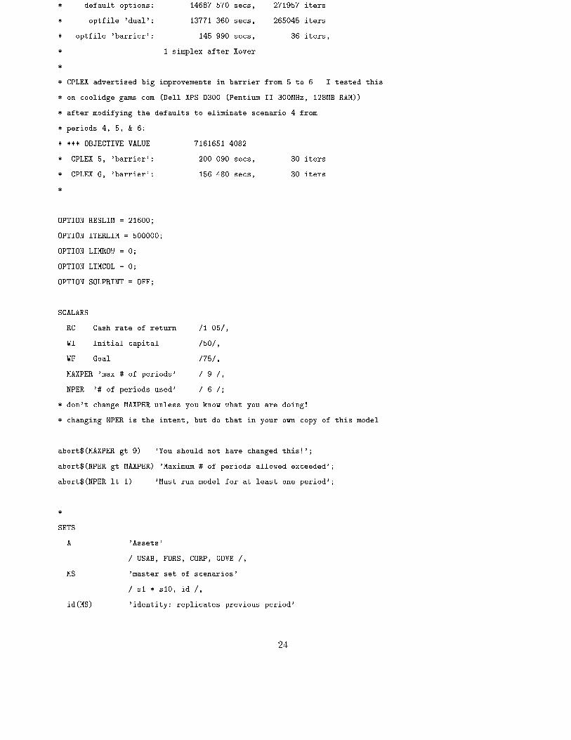
* default options: 14687.570 secs, 271957 iters

* optfile 'dual': 13771.360 secs, 265045 iters

* optfile 'barrier': 145.990 secs, 36 iters,

* 1 simplex after Xover

*

* CPLEX advertised big improvements in barrier from 5 to 6. I tested this

* on coolidge.gams.com (Dell XPS D300 (Pentium II 300MHz, 128MB RAM))

* after modifying the defaults to eliminate scenario 4 from

* periods 4, 5, & 6:

* *** OBJECTIVE VALUE 7161651.4082

* CPLEX 5, 'barrier': 200.090 secs, 30 iters

* CPLEX 6, 'barrier': 156.480 secs, 30 iters

*

OPTION RESLIM = 21600;

OPTION ITERLIM = 500000;

OPTION LIMROW = 0;

OPTION LIMCOL = 0;

OPTION SOLPRINT = OFF;

SCALARS

RC Cash rate of return /1.05/,

WI Initial capital /50/,

WF Goal /75/,

MAXPER 'max # of periods' / 9 /,

NPER '# of periods used' / 6 /;

* don't change MAXPER unless you know what you are doing!

* changing NPER is the intent, but do that in your own copy of this model

abort$(MAXPER gt 9) 'You should not have changed this!';

abort$(NPER gt MAXPER) 'Maximum # of periods allowed exceeded';

abort$(NPER lt 1) 'Must run model for at least one period';

*

SETS

A 'Assets'

/ USAB, FORS, CORP, GOVE /,

MS 'master set of scenarios'

/ s1 * s10, id /,

id(MS) 'identity: replicates previous period'

24

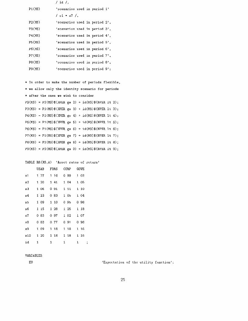
/ id /,

P1(MS) 'scenarios used in period 1'

/ s1 * s7 /,

P2(MS) 'scenarios used in period 2',







P9(MS) 'scenarios used in period 9';

* In order to make the number of periods flexible,

* we allow only the identity scenario for periods

* after the ones we wish to consider.

P2(MS) = P1(MS)$(NPER ge 2) + id(MS)$(NPER lt 2);








TABLE RR(MS,A) 'Asset rates of return'

USAB FORS CORP GOVE

s1 1.27 1.16 0.99 1.02

s2 1.20 1.41 1.04 1.05

s3 1.06 0.91 1.11 1.10

s4 1.23 0.83 1.05 1.04

s5 1.09 1.10 0.95 0.98

s6 1.15 1.28 1.25 1.18

s7 0.83 0.97 1.02 1.07

s8 0.83 0.77 0.91 0.98

s9 1.09 1.18 1.18 1.16

s10 1.20 1.18 1.18 1.16

id 1 1 1 1 ;

VARIABLES

EU 'Expectation of the utility function';

25

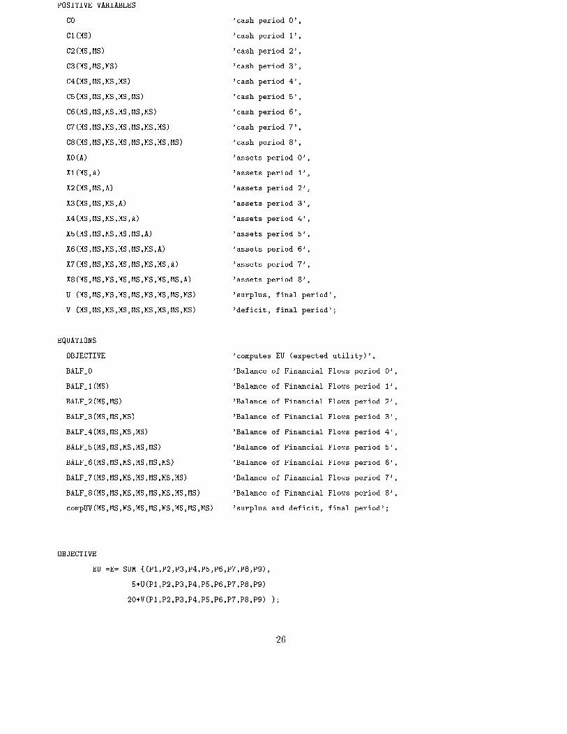
POSITIVE VARIABLES

C0 'cash period 0',

C1(MS) 'cash period 1',

C2(MS,MS) 'cash period 2',

C3(MS,MS,MS) 'cash period 3',

C4(MS,MS,MS,MS) 'cash period 4',

C5(MS,MS,MS,MS,MS) 'cash period 5',

C6(MS,MS,MS,MS,MS,MS) 'cash period 6',

C7(MS,MS,MS,MS,MS,MS,MS) 'cash period 7',

C8(MS,MS,MS,MS,MS,MS,MS,MS) 'cash period 8',

X0(A) 'assets period 0',

X1(MS,A) 'assets period 1',

X2(MS,MS,A) 'assets period 2',

X3(MS,MS,MS,A) 'assets period 3',

X4(MS,MS,MS,MS,A) 'assets period 4',

X5(MS,MS,MS,MS,MS,A) 'assets period 5',

X6(MS,MS,MS,MS,MS,MS,A) 'assets period 6',

X7(MS,MS,MS,MS,MS,MS,MS,A) 'assets period 7',

X8(MS,MS,MS,MS,MS,MS,MS,MS,A) 'assets period 8',

U (MS,MS,MS,MS,MS,MS,MS,MS,MS) 'surplus, final period',

V (MS,MS,MS,MS,MS,MS,MS,MS,MS) 'deficit, final period';

EQUATIONS

OBJECTIVE 'computes EU (expected utility)',

BALF_0 'Balance of Financial Flows period 0',

BALF_1(MS) 'Balance of Financial Flows period 1',

BALF_2(MS,MS) 'Balance of Financial Flows period 2',

BALF_3(MS,MS,MS) 'Balance of Financial Flows period 3',

BALF_4(MS,MS,MS,MS) 'Balance of Financial Flows period 4',

BALF_5(MS,MS,MS,MS,MS) 'Balance of Financial Flows period 5',

BALF_6(MS,MS,MS,MS,MS,MS) 'Balance of Financial Flows period 6',

BALF_7(MS,MS,MS,MS,MS,MS,MS) 'Balance of Financial Flows period 7',

BALF_8(MS,MS,MS,MS,MS,MS,MS,MS) 'Balance of Financial Flows period 8',

compUV(MS,MS,MS,MS,MS,MS,MS,MS,MS) 'surplus and deficit, final period';

OBJECTIVE..

EU =E= SUM {(P1,P2,P3,P4,P5,P6,P7,P8,P9),

5*U(P1,P2,P3,P4,P5,P6,P7,P8,P9)

-20*V(P1,P2,P3,P4,P5,P6,P7,P8,P9) };

26

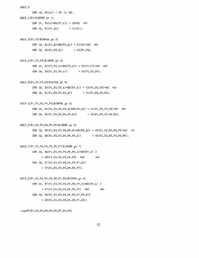
BALF_0..

SUM {A, X0(A)} + C0 =L= WI;

BALF_1(P1)$(NPER gt 1)..

SUM {A, X0(A)*RR(P1,A)} + C0*RC =E=

SUM {A, X1(P1,A)} + C1(P1);

BALF_2(P1,P2)$(NPER gt 2)..

SUM {A, X1(P1,A)*RR(P2,A)} + C1(P1)*RC =E=

SUM {A, X2(P1,P2,A)} + C2(P1,P2);

BALF_3(P1,P2,P3)$(NPER gt 3)..

SUM {A, X2(P1,P2,A)*RR(P3,A)} + C2(P1,P2)*RC =E=

SUM {A, X3(P1,P2,P3,A)} + C3(P1,P2,P3);

BALF_4(P1,P2,P3,P4)$(NPER gt 4)..

SUM {A, X3(P1,P2,P3,A)*RR(P4,A)} + C3(P1,P2,P3)*RC =E=

SUM {A, X4(P1,P2,P3,P4,A)} + C4(P1,P2,P3,P4);

BALF_5(P1,P2,P3,P4,P5)$(NPER gt 5)..

SUM {A, X4(P1,P2,P3,P4,A)*RR(P5,A)} + C4(P1,P2,P3,P4)*RC =E=

SUM {A, X5(P1,P2,P3,P4,P5,A)} + C5(P1,P2,P3,P4,P5);

BALF_6(P1,P2,P3,P4,P5,P6)$(NPER gt 6)..

SUM {A, X5(P1,P2,P3,P4,P5,A)*RR(P6,A)} + C5(P1,P2,P3,P4,P5)*RC =E=

SUM {A, X6(P1,P2,P3,P4,P5,P6,A)} + C6(P1,P2,P3,P4,P5,P6);

BALF_7(P1,P2,P3,P4,P5,P6,P7)$(NPER gt 7)..

SUM {A, X6(P1,P2,P3,P4,P5,P6,A)*RR(P7,A) }

+ C6(P1,P2,P3,P4,P5,P6) *RC =E=

SUM {A, X7(P1,P2,P3,P4,P5,P6,P7,A)}

+ C7(P1,P2,P3,P4,P5,P6,P7);

BALF_8(P1,P2,P3,P4,P5,P6,P7,P8)$(NPER gt 8)..

SUM {A, X7(P1,P2,P3,P4,P5,P6,P7,A)*RR(P8,A) }

+ C7(P1,P2,P3,P4,P5,P6,P7) *RC =E=

SUM {A, X8(P1,P2,P3,P4,P5,P6,P7,P8,A)}

+ C8(P1,P2,P3,P4,P5,P6,P7,P8);

compUV(P1,P2,P3,P4,P5,P6,P7,P8,P9)..

27

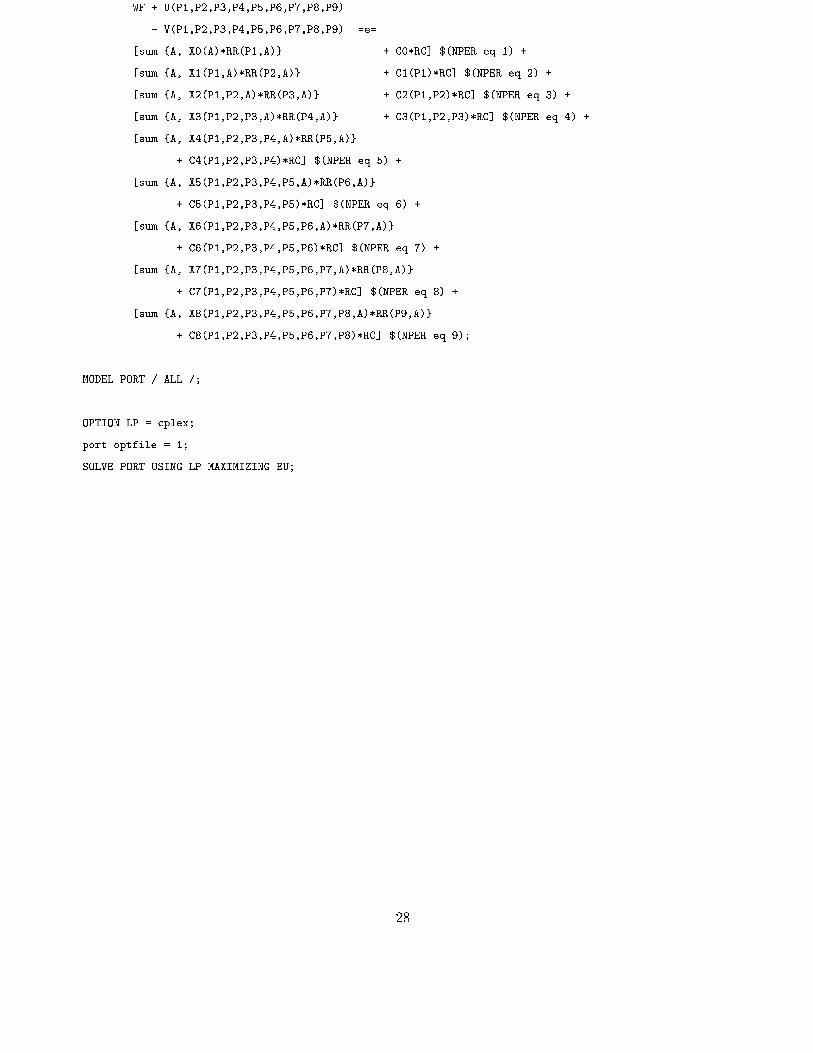
WF + U(P1,P2,P3,P4,P5,P6,P7,P8,P9)

- V(P1,P2,P3,P4,P5,P6,P7,P8,P9) =e=

[sum {A, X0(A)*RR(P1,A)} + C0*RC] $(NPER eq 1) +

[sum {A, X1(P1,A)*RR(P2,A)} + C1(P1)*RC] $(NPER eq 2) +

[sum {A, X2(P1,P2,A)*RR(P3,A)} + C2(P1,P2)*RC] $(NPER eq 3) +

[sum {A, X3(P1,P2,P3,A)*RR(P4,A)} + C3(P1,P2,P3)*RC] $(NPER eq 4) +

[sum {A, X4(P1,P2,P3,P4,A)*RR(P5,A)}

+ C4(P1,P2,P3,P4)*RC] $(NPER eq 5) +

[sum {A, X5(P1,P2,P3,P4,P5,A)*RR(P6,A)}

+ C5(P1,P2,P3,P4,P5)*RC] $(NPER eq 6) +

[sum {A, X6(P1,P2,P3,P4,P5,P6,A)*RR(P7,A)}

+ C6(P1,P2,P3,P4,P5,P6)*RC] $(NPER eq 7) +

[sum {A, X7(P1,P2,P3,P4,P5,P6,P7,A)*RR(P8,A)}

+ C7(P1,P2,P3,P4,P5,P6,P7)*RC] $(NPER eq 8) +

[sum {A, X8(P1,P2,P3,P4,P5,P6,P7,P8,A)*RR(P9,A)}

+ C8(P1,P2,P3,P4,P5,P6,P7,P8)*RC] $(NPER eq 9);

MODEL PORT / ALL /;

OPTION LP = cplex;

port.optfile = 1;

SOLVE PORT USING LP MAXIMIZING EU;

28

building and solving large-scale stochastic programs on an affordable distributed computing

Documents