pysp: modeling and solving stochastic programs in … manuscript no. (will be inserted by the...

Noname manuscript No.(will be inserted by the editor)

PySP: Modeling and Solving Stochastic Programs inPython

Jean-Paul Watson · David L. Woodruff ·William E. Hart

Received: September 6, 2010.

Abstract Although stochastic programming is a powerful tool for modeling decision-

making under uncertainty, various impediments have historically prevented its wide-

spread use. One key factor involves the ability of non-specialists to easily express

stochastic programming problems as extensions of deterministic models, which are

often formulated first. A second key factor relates to the difficulty of solving stochastic

programming models, particularly the general mixed-integer, multi-stage case. Intri-

cate, configurable, and parallel decomposition strategies are frequently required to

achieve tractable run-times. We simultaneously address both of these factors in our

PySP software package, which is part of the COIN-OR Coopr open-source Python

project for optimization. To formulate a stochastic program in PySP, the user speci-

fies both the deterministic base model and the scenario tree with associated uncertain

parameters in the Pyomo open-source algebraic modeling language. Given these two

models, PySP provides two paths for solution of the corresponding stochastic program.

The first alternative involves writing the extensive form and invoking a standard deter-

ministic (mixed-integer) solver. For more complex stochastic programs, we provide an

implementation of Rockafellar and Wets’ Progressive Hedging algorithm. Our particu-

lar focus is on the use of Progressive Hedging as an effective heuristic for approximating

Jean-Paul WatsonSandia National LaboratoriesDiscrete Math and Complex Systems DepartmentPO Box 5800, MS 1318Albuquerque, NM 87185-1318E-mail: [email protected]

David L. WoodruffGraduate School of ManagementUniversity of California DavisDavis, CA 95616-8609E-mail: [email protected]

William E. HartSandia National LaboratoriesComputer Science and Informatics DepartmentPO Box 5800, MS 1318Albuquerque, NM 87185-1318E-mail: [email protected]

2

general multi-stage, mixed-integer stochastic programs. By leveraging the combination

of a high-level programming language (Python) and the embedding of the base deter-

ministic model in that language (Pyomo), we are able to provide completely generic

and highly configurable solver implementations. PySP has been used by a number of

research groups, including our own, to rapidly prototype and solve difficult stochastic

programming problems.

1 Introduction

The modeling of uncertainty is widely recognized as an integral component in most

real-world decision problems. Typically, uncertainty is associated with the problem

input parameters, e.g., consumer demands or construction times. In cases where pa-

rameter uncertainty is independent of the decisions, stochastic programming is an

appropriate and widely studied mathematical framework to express and solve uncer-

tain decision problems [Birge and Louveaux, 1997, Wallace and Ziemba, 2005, Kall

and Mayer, 2005a, Shapiro et al., 2009]. However, stochastic programming has not yet

seen widespread, routine use in industrial applications – despite the significant bene-

fit such techniques can confer over deterministic mathematical programming models.

The growing practical importance of stochastic programming is underscored by the re-

cent proposals for and additions of capabilities in many commercial algebraic modeling

languages [AIMMS, Valente et al., 2009, Xpress-Mosel, 2010, Maximal Software, 2010].

Over the past decade, two key impediments have been informally recognized as

central in inhibiting the widespread industrial use of stochastic programming. First,

modeling systems for mathematical programming have only recently begun to incorpo-

rate extensions for specifying stochastic programs. Without an integrated and acces-

sible modeling capability, practitioners are forced to implement custom techniques for

specifying stochastic programs. Second, stochastic programs are often extremely diffi-

cult to solve – especially in contrast to their deterministic mixed-integer counterparts.

There exists no analog to CPLEX [CPLEX, 2010], Gurobi [GUROBI, 2010], Maximal

[Maximal Software, 2010], or XpressMP [XpressMP, 2010] for stochastic programming,

principally because the algorithmic technology is still under active investigation and

development, particularly in the multi-stage and mixed-integer cases.

Some commercial vendors have recently introduced modeling capabilities for stochas-

tic programming, e.g., LINDO Systems [LINDO, 2010], FICO [XpressMP, 2010], and

AIMMS [AIMMS]. On the open-source front, the options are even more limited. FLOPC++

(part of COIN-OR) [FLOPCPP, 2010] provides an algebraic modeling environment in

C++ that allows for specification of stochastic linear programs. APLEpy provides sim-

ilar functionality in a Python programming language environment. In either case, the

available modeling extensions have not yet seen widespread adoption.

The landscape for solvers (open-source or otherwise) devoted to generic stochas-

tic programs is extremely sparse. Those modeling packages that do provide stochastic

programming facilities with few exceptions rely on the translation of problem into

the extensive form – a deterministic mathematical programming representation of the

stochastic program in which all scenarios are explicitly represented and solved simulta-

neously. The extensive form can then be supplied as input to a standard (mixed-integer)

linear solver. Unfortunately, direct solution of the extensive form is unrealistic in all but

the simplest cases. Some combination of either the number of scenarios, the number of

decision stages, or the presence of discrete decision variables typically leads to extensive

3

forms that are either too difficult to solve or exhaust available system memory. Itera-

tive decomposition strategies such as the L-shaped method [Slyke and Wets, 1969] or

Progressive Hedging [Rockafellar and Wets, 1991] directly address both of these scala-

bility issues, but introduce fundamental parameters and algorithmic challenges. Other

approaches include coordinated branch-and-cut procedures [Alonso-Ayuso et al., 2003].

In general, the solution of difficult stochastic programs requires both experimentation

with and customization of alternative algorithmic paradigms – necessitating the need

for generic and configurable solvers.

In this paper, we describe an open-source software package – PySP – that begins

to address the issue of the availability of generic and customizable stochastic pro-

gramming solvers. At the same time, we describe modeling capabilities for expressing

stochastic programs. Beyond the obvious need to somehow express a problem instance

to a solver, we identify a fundamental characteristic of the modeling language that is in

our opinion necessary to achieve the objective of generic and customizable stochastic

programming solvers. In particular, the modeling layer must provide mechanisms for

accessing components via direct introspection [Python, 2010b], such that solvers can

generically and programmatically access and manipulate model components. Further,

from a user standpoint, the modeling layer should differentiate between abstract mod-

els and model instances – following best practices from the deterministic mathematical

modeling community [Fourer et al., 1990].

To express a stochastic program in PySP, the user specifies both the deterministic

base model and the scenario tree model with associated uncertain parameters in the

Pyomo open-source algebraic modeling language [Hart et al., 2010]. This separation of

deterministic and stochastic problem components is similar to the mechanism proposed

in SMPS [Birge et al., 1987, Gassmann and Schweitzer, 2001]. Pyomo is a Python-

based modeling language, and provides the ability to model both abstract problems

and concrete problem instances. The embedding of Pyomo in Python enables model

introspection and the construction of generic solvers.

Given the deterministic and scenario tree models, PySP provides two paths for the

solution of the corresponding stochastic program. The first alternative involves writ-

ing the extensive form and invoking a deterministic (mixed-integer) linear solver. For

more complex stochastic programs, we provide a generic implementation of Rockafellar

and Wets’ Progressive Hedging algorithm [Rockafellar and Wets, 1991]. Our particular

focus is on the use of Progressive Hedging as an effective heuristic for approximating

general multi-stage, mixed-integer programs. By leveraging the combination of a high-

level programming language (Python) and the embedding of the base deterministic

model in that language (Pyomo), we are able to provide completely generic and highly

configurable solver implementations. Karabuk and Grant [2007] describe the benefits

of Python for such model-building and solving in more detail.

The remainder of this paper is organized as follows. We begin in Section 2 with a

brief overview of stochastic programming, focusing on multi-stage notation and expres-

sion of the scenario tree. In Section 3, we describe the PySP approach to modeling a

stochastic program, illustrated using a well-known introductory model. PySP capabili-

ties for writing and solving the extensive form are described in Section 4. In Section 5,

we compare and contrast PySP with other open-source software packages for modeling

and solving stochastic programs. Our generic implementation of Progressive Hedging is

described in Section 6, while Section 7 details mechanisms for customizing the behavior

of PH. By basing PySP on Coopr and Python, we are able to provide straightforward

mechanisms to support distributed parallel solves in the context of PH and other de-

4

composition algorithms; these facilities are detailed in Section 8. Finally, we conclude

in Section 9, with a brief discussion of the use of PySP on a number of active research

projects.

2 Stochastic Programming: Definition and Notations

PySP is designed to express and solve stochastic programming problems, which we

now briefly introduce. More comprehensive introductions to both the theoretical foun-

dations and the range of potential applications can be found in [Birge and Louveaux,

1997], [Shapiro et al., 2009], and [Wallace and Ziemba, 2005].

We concern ourselves with stochastic optimization problems where uncertain pa-

rameters (data) can be represented by a set of scenarios S, each of which specifies

both (1) a full set of random variable realizations and (2) a corresponding probabil-

ity of occurrence. The random variables in question specify the evolution of uncertain

parameters over time. We index the scenario set by s and refer to the probability of

occurrence of s (or, more accurately, a realization “near” scenario s) as Pr(s). Let the

number of scenarios be given by |S|. The source of these scenarios does not concern us

in this paper, although we observe that they are frequently obtained via simulation or

formed from expert opinions. We assume that the decision process of interest consists

of a sequence of discrete time stages, the set of which is denoted T . We index T by t,

and denote the number of time stages by |T |.Although PySP can support some types of non-linear constraints and objectives,

we develop the notation primarily for the linear case in the interest of simplicity. For

each scenario s and time stage t, t ∈ 1, . . . , |T |, we are given a row vector c(s, t)

of length n(t), a m(t) × n(t) matrix A(s, t), and a column vector b(s, t) of length

m(t). Let N(t) be the index set 1, . . . , n(t) and M(t) be the index set 1, . . . , m(t).For notational convenience, let A(s) denote (A(s, 1), . . . , A(s, |T |)) and let b(s) denote

(b(s, 1), . . . , b(s, |T |)).The decision variables in a stochastic program consist of a set of n(t) vectors x(t);

one vector for each scenario s ∈ S. Let X(s) be (x(s, 1), . . . , x(s, T )). We will use X as

shorthand for the entire solution system of x vectors, i.e., X = x(1, 1), . . . , x(|S|, |T |).If we were prescient enough to know which scenario s ∈ S would be ultimately

realized, our optimization objective would be to minimize

fs(X(s)) ≡∑t∈T

∑i∈N(t)

[ci(s, t)xi(s, t)] (Ps)

subject to the constraint

X ∈ Ωs.

We use Ωs as an abstract notation to express all constraints for scenario s, including

requirements that some decision vector elements are discrete or more general require-

ments such as

A(s)X(s) ≥ b(s).

The notation A(s)X(s) is used to capture the usual sorts of single period and inter-

period linking constraints that one typically finds in multi-stage mathematical pro-

gramming formulations.

We must obtain solutions that do not require foreknowledge and that will be feasible

independent of which scenario is ultimately realized. In particular, lacking prescience,

5

only solutions that are implementable are practically useful. Solutions that are not

admissible, on the other hand, may have some value because while some constraints may

represent laws of physics, others may be violated slightly without serious consequence.

We refer to a solution that satisfies constraints for all scenarios as admissible. We

refer to a solution vector as implementable if for all pairs of scenario s and s′ that

are indistinguishable up to time t, xi(s, t′) = xi(s

′, t′) for all 1 ≤ t′ ≤ t and each i in

each N(t). We refer to the set of all implementable solutions as NS for a given set of

scenarios, S.

To achieve admissible and implementable solutions, the expected value minimiza-

tion problem then becomes:

min∑s∈S

[Pr(s)f(s; X(s))] (P)

subject to

X ∈ Ωs

X ∈ NS .

Formulation (P) is known as a stochastic mathematical program. If all decision

variables are continuous, we refer to the problem simply as a stochastic program. If

some of the decision variables are discrete, we refer to the problem as a stochastic

mixed-integer program.

In practice, the parameter uncertainty is stochastic programs is often encoded via a

scenario tree, in which a node specifies the parameter values b(s, t), c(s, t), and A(s, t)

for all t ∈ T and s, s′ ∈ S such that s and s′ are indistinguishable up to time t. Scenario

trees are discussed in more detail in Section 6.

3 Modeling in PySP

Modern algebraic modeling languages (AMLs) such as AMPL [AMPL, 2010] and

GAMS [GAMS, 2010] provide powerful mechanisms for expressing and solving deter-

ministic mathematical programs. AMLs allow non-specialists to easily formulate and

solve mathematical programming models, avoiding the need for a deep understanding

of the underlying algorithmic technologies; we desire to retain the same capabilities

for stochastic mathematical programming models. Many AMLs differentiate between

the abstract, symbolic model and a concrete instance of the model, i.e., a model in-

stantiated with data. The advantages of this approach are widely known [Fourer et al.,

1990, p.35]. Thus, a design objective is to retain this differentiation in our approach

to modeling stochastic mathematical programs in PySP. Finally, our ultimate objec-

tive is to develop and maintain software under an open-source distribution license.

Consequently, PySP itself must be based on an open-source AML.

These design requirements have led us to select Pyomo [Hart et al., 2010] as the

AML on which to base PySP. Pyomo is an open-source AML developed and main-

tained by Sandia National Laboratories (co-developed by authors of this paper), and is

distributed as part of the COIN-OR initiative [COIN-OR, 2010]. Pyomo is written in

the Python high-level programming language [Python, 2010a], which possesses several

features that enable the development of generic solvers. AML alternatives to Pyomo

6

(many of which are also written in Python) do exist, but the discussion of the pros and

cons are beyond the present scope; we defer to [Hart et al., 2010] for such arguments.

In this section, we discuss the use of Pyomo to formulate and express stochastic

programs in PySP. As a motivating example, we consider the well-known Birge and

Louveaux [Birge and Louveaux, 1997] “farmer” stochastic program. Mirroring several

other approaches to modeling stochastic programs (e.g., see [Thenie et al., 2007]), we

require the specification of two related components: the deterministic base model and

the scenario tree. In Section 3.1 we discuss the specification of the deterministic ref-

erence model and associated data; Section 3.2 details the model and data underlying

PySP scenario tree specification. The mechanisms for specifying uncertain parameter

data are discussed in Section 3.3. Finally, we briefly discuss the programmatic com-

pilation of a scenario tree specification into objects appropriate for use by solvers in

Section 3.4.

3.1 The Deterministic Reference Model

The starting point for developing a stochastic programming model in PySP is the

specification of an abstract reference model, which describes the deterministic multi-

stage problem for an representative scenario. The reference model does not make use

of, or describe, any information relating to parameter uncertainty or the scenario tree.

Typically, it is simply the model that would be used in single-scenario analysis, i.e.,

the model that is commonly developed before stochastic aspects of an optimization

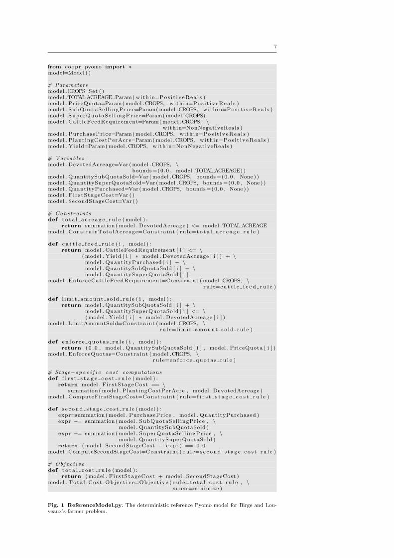
problem are considered. PySP requires that the reference model – specified in Pyomo

– is contained in a file named ReferenceModel.py. As an illustrative example, the

complete reference model for Birge and Louveaux’s farmer problem is shown Figure 1.

When looking at this figure, it is useful to remember that backslash is the python line

continuation character.

For details concerning the syntax and use of the Pyomo language, we defer to

[Hart et al., 2010]. Here, we simply observe that a detailed knowledge of Python is

not necessary to develop a reference model in Pyomo; users are often unaware that a

Pyomo model specifies executable Python code, or that they are using a class library.

Relative to the AMPL formulation of the farmer problem, the Pyomo formulation is

somewhat more verbose – primarily due to its embedding in an high-level programming

language.

While the reference model is independent of any stochastic components of the

problem, PySP does require that the objective cost component for each decision stage

of the stochastic program be assigned to a distinct variable or variable index. In the

farmer reference model, we simply label the first and second stage cost variables as

FirstStageCost and SecondStageCost, respectively. The corresponding values are com-

puted via the constraints ComputeFirstStageCost and ComputeSecondStageCost. We

initially imposed the requirement concerning specification of per-stage cost variables

(which are not a common feature in other stochastic programming software packages)

primarily to facilitate various aspects of solution reporting. However, the convention

has additionally proved very useful in implementation of various PySP solvers.

To create a concrete instance from the abstract reference model, a Pyomo data file

must also be specified. The data can correspond to an arbitrary scenario, and must

completely specify all parameters in the abstract reference model. The reference data

file must be named ReferenceModel.dat. An example data file corresponding to the

7

from coopr . pyomo import ∗model=Model ( )

# Parametersmodel .CROPS=Set ( )model .TOTAL ACREAGE=Param( with in=Pos i t i v eRea l s )model . PriceQuota=Param( model .CROPS, with in=Pos i t i v eRea l s )model . SubQuotaSe l l ingPr ice=Param( model .CROPS, with in=Pos i t i v eRea l s )model . SuperQuotaSe l l ingPr i ce=Param( model .CROPS)model . CattleFeedRequirement=Param( model .CROPS, \

with in=NonNegativeReals )model . PurchasePr ice=Param( model .CROPS, with in=Pos i t i v eRea l s )model . PlantingCostPerAcre=Param( model .CROPS, with in=Pos i t i v eRea l s )model . Yie ld=Param( model .CROPS, with in=NonNegativeReals )

# Variab l e smodel . DevotedAcreage=Var ( model .CROPS, \

bounds =(0.0 , model .TOTAL ACREAGE))model . QuantitySubQuotaSold=Var ( model .CROPS, bounds =(0.0 , None ) )model . QuantitySuperQuotaSold=Var ( model .CROPS, bounds =(0.0 , None ) )model . QuantityPurchased=Var ( model .CROPS, bounds =(0.0 , None ) )model . F i r s tStageCost=Var ( )model . SecondStageCost=Var ( )

# Constra in tsdef t o t a l a c r e a g e r u l e ( model ) :

return summation ( model . DevotedAcreage ) <= model .TOTAL ACREAGEmodel . Constra inTotalAcreage=Constra int ( r u l e=t o t a l a c r e a g e r u l e )

def c a t t l e f e e d r u l e ( i , model ) :return model . CattleFeedRequirement [ i ] <= \

( model . Yie ld [ i ] ∗ model . DevotedAcreage [ i ] ) + \model . QuantityPurchased [ i ] − \model . QuantitySubQuotaSold [ i ] − \model . QuantitySuperQuotaSold [ i ]

model . EnforceCatt leFeedRequirement=Constra int ( model .CROPS, \r u l e=c a t t l e f e e d r u l e )

def l im i t amoun t s o l d ru l e ( i , model ) :return model . QuantitySubQuotaSold [ i ] + \

model . QuantitySuperQuotaSold [ i ] <= \( model . Yie ld [ i ] ∗ model . DevotedAcreage [ i ] )

model . LimitAmountSold=Constra int ( model .CROPS, \r u l e=l im i t amoun t s o l d ru l e )

def e n f o r c e qu o t a s r u l e ( i , model ) :return ( 0 . 0 , model . QuantitySubQuotaSold [ i ] , model . PriceQuota [ i ] )

model . EnforceQuotas=Constra int ( model .CROPS, \r u l e=en f o r c e qu o t a s r u l e )

# Stage−s p e c i f i c co s t computationsdef f i r s t s t a g e c o s t r u l e ( model ) :

return model . F i r s tStageCost == \summation ( model . PlantingCostPerAcre , model . DevotedAcreage )

model . ComputeFirstStageCost=Constra int ( r u l e=f i r s t s t a g e c o s t r u l e )

def s e c o nd s t a g e c o s t r u l e ( model ) :expr=summation ( model . PurchasePrice , model . QuantityPurchased )expr −= summation ( model . SubQuotaSel l ingPrice , \

model . QuantitySubQuotaSold )expr −= summation ( model . SuperQuotaSe l l ingPr ice , \

model . QuantitySuperQuotaSold )return ( model . SecondStageCost − expr ) == 0 .0

model . ComputeSecondStageCost=Constra int ( r u l e=s e c o nd s t a g e c o s t r u l e )

# Objec t i v edef t o t a l c o s t r u l e ( model ) :

return ( model . F i r s tStageCost + model . SecondStageCost )model . Tota l Cos t Objec t ive=Object ive ( r u l e=t o t a l c o s t r u l e , \

s ense=minimize )

Fig. 1 ReferenceModel.py: The deterministic reference Pyomo model for Birge and Lou-veaux’s farmer problem.

8

s e t CROPS := WHEAT CORN SUGAR BEETS ;

param TOTAL ACREAGE := 500 ;

param PriceQuota := WHEAT 100000 CORN 100000 SUGAR BEETS 6000 ;

param SubQuotaSe l l ingPr ice := WHEAT 170 CORN 150 SUGAR BEETS 36 ;

param SuperQuotaSe l l ingPr i ce := WHEAT 0 CORN 0 SUGAR BEETS 10 ;

param CattleFeedRequirement := WHEAT 200 CORN 240 SUGAR BEETS 0 ;

param PurchasePr ice := WHEAT 238 CORN 210 SUGAR BEETS 100000 ;

param PlantingCostPerAcre := WHEAT 150 CORN 230 SUGAR BEETS 260 ;

param Yie ld := WHEAT 3.0 CORN 3.6 SUGAR BEETS 24 ;

Fig. 2 ReferenceModel.dat: The Pyomo reference model data for Birge and Louveaux’sfarmer problem.

farmer reference model is shown in Figure 2. Although Pyomo supports various data

file formats, the example illustrates the use of a file that uses Pyomo data commands

– the most commonly used data file format in Pyomo. Pyomo data commands include

data commands for set and parameter data that are consistent with AMPL’s data

commands. Our adoption of this convention minimizes the effort required to translate

deterministic reference models expressed in AMPL into Pyomo.

3.2 The Scenario Tree

Given a deterministic reference model, the second step in developing a stochastic pro-

gram in PySP involves specification of the scenario tree structure and associated pa-

rameter data. A PySP scenario tree specification supplies all information concern-

ing the time stages, the mapping of decision variables to time stages, how various

scenarios are temporally related to one another (i.e., scenario tree nodes and their

inter-relationships), and the probabilities of various scenarios. As discussed below, the

scenario tree does not directly specify uncertain parameter values; rather, it specifies

references to data files containing such data.

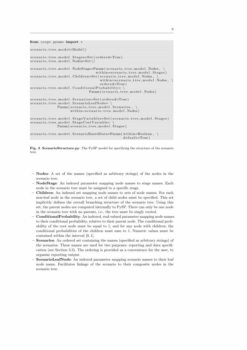
As with the abstract reference model, the abstract scenario tree model in PySP is

expressed in Pyomo. However, the contents of the scenario tree model – called Scenar-

ioStructure.py and shown in Figure 3 for reference – are fixed. The model is built

into and distributed with PySP; the user does not edit this file. Instead, the user must

supply values for each of the parameters specified in the scenario tree model. Finally,

we observe that the scenario tree model is simply a data collection that is specified

using Pyomo parameter and set objects, i.e., a very restricted form of a Pyomo model

(lacking variables, constraints, and an objective).

The precise semantics for each of the parameters (or sets) indicated in Figure 3 are

as follows:

– Stages: An ordered set containing the names (specified as arbitrary strings) of the

time stages. The order corresponds to the time order of the stages.

9

from coopr . pyomo import ∗

s c ena r i o t r e e mode l=Model ( )

s c ena r i o t r e e mode l . Stages=Set ( ordered=True )s c ena r i o t r e e mode l . Nodes=Set ( )

s c ena r i o t r e e mode l . NodeStage=Param( s c ena r i o t r e e mode l . Nodes , \with in=s c ena r i o t r e e mode l . Stages )

s c ena r i o t r e e mode l . Chi ldren=Set ( s c ena r i o t r e e mode l . Nodes , \with in=s c ena r i o t r e e mode l . Nodes , \ordered=True )

s c ena r i o t r e e mode l . Cond i t i ona lProbab i l i t y= \Param( s c ena r i o t r e e mode l . Nodes )

s c ena r i o t r e e mode l . S c ena r i o s=Set ( ordered=True )s c ena r i o t r e e mode l . ScenarioLeafNode= \

Param( s c ena r i o t r e e mode l . Scenar ios , \with in=s c ena r i o t r e e mode l . Nodes )

s c ena r i o t r e e mode l . S tageVar iab l e s=Set ( s c ena r i o t r e e mode l . Stages )s c ena r i o t r e e mode l . StageCostVar iab le= \

Param( s c ena r i o t r e e mode l . Stages )

s c ena r i o t r e e mode l . ScenarioBasedData=Param( with in=Boolean , \de f au l t=True )

Fig. 3 ScenarioStructure.py: The PySP model for specifying the structure of the scenariotree.

– Nodes: A set of the names (specified as arbitrary strings) of the nodes in the

scenario tree.

– NodeStage: An indexed parameter mapping node names to stage names. Each

node in the scenario tree must be assigned to a specific stage.

– Children: An indexed set mapping node names to sets of node names. For each

non-leaf node in the scenario tree, a set of child nodes must be specified. This set

implicitly defines the overall branching structure of the scenario tree. Using this

set, the parent nodes are computed internally to PySP. There can only be one node

in the scenario tree with no parents, i.e., the tree must be singly rooted.

– ConditionalProbability: An indexed, real-valued parameter mapping node names

to their conditional probability, relative to their parent node. The conditional prob-

ability of the root node must be equal to 1, and for any node with children, the

conditional probabilities of the children must sum to 1. Numeric values must be

contained within the interval [0, 1].

– Scenarios: An ordered set containing the names (specified as arbitrary strings) of

the scenarios. These names are used for two purposes: reporting and data specifi-

cation (see Section 3.3). The ordering is provided as a convenience for the user, to

organize reporting output.

– ScenarioLeafNode: An indexed parameter mapping scenario names to their leaf

node name. Facilitates linkage of the scenario to their composite nodes in the

scenario tree.

10

s e t Stages := F i r s tS tage SecondStage ;

s e t Nodes := RootNodeBelowAverageNodeAverageNodeAboveAverageNode ;

param NodeStage := RootNode F i r s tS tageBelowAverageNode SecondStageAverageNode SecondStageAboveAverageNode SecondStage ;

s e t Chi ldren [ RootNode ] := BelowAverageNodeAverageNodeAboveAverageNode ;

param Cond i t i ona lProbab i l i t y := RootNode 1 .0BelowAverageNode 0.33333333AverageNode 0.33333334AboveAverageNode 0.33333333 ;

s e t Scenar i o s := BelowAverageScenarioAverageScenar ioAboveAverageScenario ;

param ScenarioLeafNode := BelowAverageScenario BelowAverageNodeAverageScenar io AverageNodeAboveAverageScenario AboveAverageNode ;

s e t StageVar iab l e s [ F i r s tS tage ] := DevotedAcreage [ ∗ ] ;s e t StageVar iab l e s [ SecondStage ] := QuantitySubQuotaSold [ ∗ ]

QuantitySuperQuotaSold [ ∗ ]QuantityPurchased [ ∗ ] ;

param StageCostVar iab le := F i r s tS tage F i r s tStageCostSecondStage SecondStageCost ;

Fig. 4 The PySP ScenarioStructure.dat data file for specifying the scenario tree for thefarmer problem.

– StageVariables: An indexed set mapping stage names to sets of variable names in

the reference model. The sets of variables names indicate those variables that are

associated with the given stage. Implicitly defines the non-anticipativity constraints

that should be imposed when generating and/or solving the PySP model.

– ScenarioBasedData: A Boolean parameter specifying how the instances for each

scenario are to be constructed. The semantics for this parameter are detailed below

in Section 3.3.

Data to instantiate these parameters and sets must be provided by a user in a

file named ScenarioStructure.dat. The scenario tree structure specification for the

farmer problem is shown in Figure 4, specified using the AMPL data file format.

We observe that PySP provides a simple “slicing” syntax to specify subsets of

indexed variables. In particular, the “*” character is used to match all values in a

particular dimension of an indexed parameter. In more complex examples, variables are

typically indexed by time stage. In these cases, the slice syntax allows for very concise

11

specification of the stage-to-variable mapping. Finally, we observe that PySP makes no

assumptions regarding the linkage between time stages and variable index structure. In

particular, the time stage need not explicitly be referenced within a variable’s index set.

While this is often the case in multi-stage formulations, the convention is not universal,

e.g., as in the case of the farmer problem.

3.3 Scenario Parameter Specification

Data files specifying the deterministic and stochastic parameters for each of the sce-

narios in a PySP model can be specified in one of two ways. The simplest approach is

“scenario-based”, in which a single data file containing a complete parameter specifica-

tion is provided for each scenario. In this case, the file naming convention is as follows:

If the scenario is named ScenarioX, then the corresponding data file for the scenario

must be named ScenarioX.dat. This approach is often expedient – especially if the

scenario data are generated via simulation, as is often the case in practice. However,

there is necessarily redundancy in the encoding. Depending on the problem size and

number of scenarios, this redundancy may become excessive in terms of disk storage

and access. Scenario-based data specification is the default behavior in PySP, as indi-

cated by the default value of the ScenarioBasedData parameter in Figure 3. We note

that the listing in Figure 2 is an example of a scenario-based data specification.

Node-based parameter specification is provided as an alternative to the default

scenario-based approach, principally to eliminate storage redundancy. With node-based

specification, parameter data specific to each node in the scenario tree is specified in

a distinct data file. The naming convention is as follows: If the node is named NodeX,

then the corresponding data file for the node must be named NodeX.dat. To create

a scenario instance, data for all nodes associated with a scenario are accessed (via the

ScenarioLeafNode parameter in the scenario tree specification and the computed par-

ent node linkages). Node-based parameter encoding eliminates redundancy, although

typically at the expense of a slightly more complex instance generation process. To

enable node-based scenario initialization, a user needs to simply add the following line

to ScenarioStructure.dat:

param ScenarioBasedData := Fal se ;

In the case of the farmer problem, all parameters except for Yield are identi-

cal across scenarios. Consequently, these parameters can be placed in a file named

RootNode.dat. Then, files containing scenario-specific Yield parameter values are

specified for each second-stage leaf node (in files named AboveAverageNode.dat,

AverageNode.dat, and BelowAverageNode.dat).

3.4 Compilation of the Scenario Tree Model

The PySP scenario tree structure model is a declarative entity, merely specifying the

data associated with a scenario tree. PySP internally uses the information contained

in this model to construct a ScenarioTree object, which in turn is composed of Sce-

narioTreeNode, Stage, and Scenario objects. In aggregate, these Python objects allow

12

programmatic navigation, query, manipulation, and reporting of the scenario tree struc-

ture. While hidden from the typical user, these objects are crucial in the processes of

generating the extensive form (Section 4) and generic solvers (Section 6).

4 Generating and Solving the Extensive Form

Given a stochastic program encoded in accordance with the PySP conventions de-

scribed in Section 3, the next immediate issue of concern is its solution. The most

straightforward method to solve a stochastic program involves generating the exten-

sive form (also known as the deterministic equivalent) and then invoking a standard

deterministic (mixed-integer) programming solver, e.g., CPLEX. The extensive form

given as problem (P) in Section 2 completely specifies all scenarios and the coupling

non-anticipativity constraints at each node in the scenario tree.

In many cases, particularly when small numbers of scenarios are involved or the

decision variables are all continuous, the extensive form can be effectively solved with

off-the-shelf solvers [Parija et al., 2004]. Further, although decomposition techniques

may ultimately be needed for large, more complex models, the extensive form is usually

the first attempted method to solve a stochastic program.

In this section, we describe the use and design of facilities in PySP for generating

and solving the extensive form. Section 4.1 describes a user script for generating and

solving the extensive form; an overview of the implementation of this script is then

provided in Section 4.2.

4.1 The runef Script

PySP provides an easy-to-use script – runef – to both generate and solve the exten-

sive form of a stochastic program. We now briefly describe the primary command-line

options for this script; note that all options begin with a double dash prefix:

--help

Display all command-line options, with brief descriptions, and exits.

--verbose

Display verbose output to the standard output stream, above and beyond the usual

status output. Disabled by default.

--model-directory=MODEL_DIRECTORY

Specifies the directory in which the reference model (ReferenceModel.py) is

stored. Defaults to “.”, the current working directory.

--instance-directory=INSTANCE_DIRECTORY

Specifies the directory in which all reference model and scenario model data files

are stored. Defaults to “.”, the current working directory.

--output-file=OUTPUT_FILE

Specifies the name of the LP format output file to which the extensive form is

written. Defaults to “efout.lp”.

--solve

Directs the script to solve the extensive form after writing it. Disabled by default.

--solver=SOLVER_TYPE

Specifies the type of solver for solving the extensive form, if a solve is requested.

Defaults to “cplex”.

13

--solver-options=SOLVER_OPTIONS

Specifies solver options in keyword-value pair format, if a solve is requested.

--output-solver-log

Specifies that the output of the solver is to be echoed to the standard output stream.

Disabled by default. Useful to ascertain status for extensive forms with long solve

times.

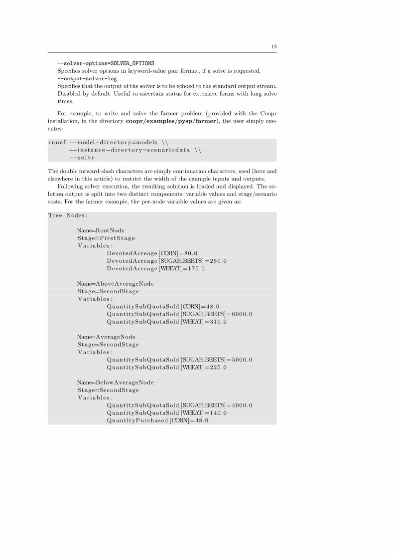
For example, to write and solve the farmer problem (provided with the Coopr

installation, in the directory coopr/examples/pysp/farmer), the user simply exe-

cutes:

rune f −−model−d i r e c t o r y=models \\−−in s tance−d i r e c t o r y=scenar i oda ta \\−−s o l v e

The double forward-slash characters are simply continuation characters, used (here and

elsewhere in this article) to restrict the width of the example inputs and outputs.

Following solver execution, the resulting solution is loaded and displayed. The so-

lution output is split into two distinct components: variable values and stage/scenario

costs. For the farmer example, the per-node variable values are given as:

Tree Nodes :

Name=RootNode

Stage=Fi r s tS tage

Var i ab l e s :

DevotedAcreage [CORN]=80.0

DevotedAcreage [SUGAR BEETS]=250.0

DevotedAcreage [WHEAT]=170.0

Name=AboveAverageNode

Stage=SecondStage

Var i ab l e s :

QuantitySubQuotaSold [CORN]=48.0

QuantitySubQuotaSold [SUGAR BEETS]=6000.0

QuantitySubQuotaSold [WHEAT]=310.0

Name=AverageNode

Stage=SecondStage

Var i ab l e s :



Name=BelowAverageNode

Stage=SecondStage

Var i ab l e s :



QuantityPurchased [CORN]=48.0

14

Similarly, the per-node stage cost and per-scenario overall costs are given as follows:

Tree Nodes :

Name=RootNode

Stage=Fi r s tS tage

Expected node co s t =−108390.0000

Name=AboveAverageNode

Stage=SecondStage


Name=AverageNode

Stage=SecondStage


Name=BelowAverageNode

Stage=SecondStage


Scenar i o s :

Name=AboveAverageScenario

Stage=F i r s tS tage Cost=108900.0000

Stage=SecondStage Cost=−275900.0000

Total s c ena r i o co s t =−167000.0000

Name=AverageScenar io




Name=BelowAverageScenario




Currently, the extensive form is output for solution in the CPLEX LP file format.

In practice, this has not been a limitation, as nearly all commercial and open-source

solvers support this format.

Various other command-line options are available in the runef script, including

those related to performance profiling and Python garbage collection. Further, the

runef script is capable of writing and solving the extensive form augmented with a

weighted Conditional Value-at-Risk term in the objective [Schultz and Tiedemann,

2005].

We conclude by noting that the runef script, as with the decomposition-based

solver script described in Section 6, relies on significant functionality from the Coopr

Python optimization library in which PySP is embedded. This includes a wide range of

15

solver interfaces (both commercial and open-source), problem writers, solution readers,

and distributed solvers. For further details, we refer to [Hart et al., 2010].

4.2 Under the Hood: Generating the Extensive Form

We now provide an overview of the implementation of the runef script. In doing so, our

objectives are to (1) illustrate the use of Python to create generic writers and solvers

and (2) to provide some indication of the programmatic-level functionality available in

PySP.

The high-level process executed by the runef script to generate the extensive form

in PySP is as follows:

1. Load the scenario tree data; create the corresponding instance.

2. Create the ScenarioTree object from the scenario tree Pyomo model.

3. Load the reference model; create the corresponding instance from reference data.

4. Load the scenario instance data; create the corresponding instances.

5. Create the master “binding” instance; instantiate per-node variable objects.

6. Add master-to-scenario instance equality constraints to enforce non-anticipativity.

Steps 1 and 2 simply involve the process of creating the Pyomo instance specifying

all data related to the scenario tree structure, and creating the corresponding Scenari-

oTree object to facilitate programmatic access of scenario tree attributes. In Step 3, the

core deterministic abstract model is loaded. The abstract model is then used in Step 4,

in conjunction with the ScenarioTree object, to create a concrete model instance for

each scenario in the stochastic program. The scenario instances are at this point –

and remain so – completely independent of one another. This approach differs from

that of some of the software packages described in Section 5, in which variables are

instantiated for each node of the scenario tree and shared across the relevant scenarios.

While our approach does introduce redundancy, the replication introduces only moder-

ate memory overhead and confers significant practical advantages when implementing

generic decomposition-based solvers, e.g., as illustrated below in Section 6. In partic-

ular, we note that scenario-based decomposition solvers gradually and incrementally

enforce non-anticipativity, such that replicated variables are required.

Next, a master “binding” instance is created in Steps 5 and 6. The purpose of the

master binding instance is to enforce the required non-anticipativity constraints at each

node in the scenario tree. Using the ScenarioTree object, the tree is traversed and the

collection of variable names (including indicies, if necessary) associated with each node

is identified – initially specified via the StageVariables attribute of the scenario tree

model. The corresponding variable objects are then identified in the reference model

instance, cloned, and attached to the binding instance. This step critically requires

the Python capability of introspection: the ability, at run-time, to gather information

about objects and manipulate them.

To illustrate how introspection is used to develop generic algorithms, consider again

the farmer example from Section 3. By specifying the line

s e t StageVar iab l e s [ F i r s tS tage ] := DevotedAcreage [ ∗ ] ;

16

the user is communicating the requirement to impose non-anticipativity constraints on

(all indices of) the first stage variable DevotedAcreage. The variable is specified simply

as a string, which can be programmatically split into the corresponding root name

and index template. Using the root name, Python can query (via the getattr built-in

function) the reference model for the corresponding variable, validate that it exists,

and if so, return the corresponding variable object. This loose coupling between the

user data and algorithm code is facilitated by this simple, yet powerful, introspection

mechanism.

The final primary step in the runef script involves construction of constraints to

enforce non-anticipativity between the newly created variables in the master binding

instance and the variables in the relevant scenario instances. This process again relies

on introspection to achieve a generic implementation.

Overall, the core functionality of the runef script is expressed in approximately 700

lines of Python code – including all white-space and comments. This includes both the

code for creating the relevant Pyomo instances, generating the master binding instance

via the processed described above, and controlling the output of the LP file.

Finally, we observe that despite our explicit approach to writing the extensive form

through the introduction of master variables and non-anticipativity constraints, we

find that the impact on run-time is at worst negligible. The presolvers in commer-

cial packages such as CPLEX, Gurobi, or XpressMP (and those available with some

open-source solvers) are able to quickly identify and eliminate most of the redundant

variables and constraints.

5 Related Proposals and Software Packages

We now briefly survey prior and on-going efforts to develop software packages support-

ing the specification and solution of stochastic programs, with the objective of placing

the capabilities of PySP in this broader context. Numerous extensions to existing AMLs

to support the specification of stochastic programs have been proposed in the literature;

Gassmann and Ireland [1996] is an early example. Similarly, various solver interfaces

have been proposed, with the dominant mechanism being the direct solution of the

extensive form. Here, we primarily focus on specification and solver efforts associated

with open-source and academic initiatives, which generally share the same distribution

goals, user community targets, and design objectives (e.g., experimental, generic, and

configurable solvers) as PySP.

StAMPL Fourer and Lopes [2009] describe an extension to AMPL, called StAMPL,

whose goal is to simplify the modeling process associated with stochastic program spec-

ification. One key objective of StAMPL is to explicitly avoid the use of scenario and

stage indices when specifying the core algebraic model, separating the specification of

the stochastic process from the underlying deterministic optimization model. The au-

thors describe a preprocessor that translates a StAMPL problem description into the

fully indexed AMPL model, which in turn is written in SMPS format for solution. In

contrast to StAMPL, PySP provides a straightforward mechanism to specify a stochas-

tic program, and does not strive to advance the state-of-the-art in modeling. Rather,

our primary focus is on developing generic and configurable solvers, and discussed in

Sections 4, 6, and 7.

17

STRUMS STRUMS is a system for performing and managing decomposition and re-

laxation strategies in stochastic programming [Fourer and Lopes, 2006]. Input problems

are specified in the SMPS format, and the package provides mechanisms for writing the

extensive form, performing basic and nested Benders decomposition (i.e., the L-shaped

method), and implementing Lagrangian relaxation; only stochastic linear programs are

considered. The design objective of STRUM – to provide mechanisms facilitating auto-

matic problem decomposition – is consistent with the design of PySP. However, PySP

currently provides mechanisms for scenario-based decomposition, in contrast to stage-

oriented decomposition. This emphasis is due primarily to our interest in mixed-integer

stochastic programming. In contrast to STRUMS, PySP is integrated with an AML.

DET2STO Thenie et al. [2007] describe an extension of AMPL to support the spec-

ification of stochastic programs, noting that (at the time the effort was initiated) no

AMLs were available with stochastic programming support. In particular, they pro-

vide a script – called DET2STO, available from http://apps.ordecsys.com/det2sto

– taking an augmented AMPL model as input and generating the extensive form via

an SMPS output file. The research focus is on the automated generation of the ex-

tensive form, with the authors noting: “We recall here that, while it is relatively easy

to describe the two base components - the underlying deterministic model and the

stochastic process - it is tedious to define the contingent variables and constraints and

build the deterministic equivalent” [Thenie et al., 2007, p.35]. While subtle modeling

differences do exist between DET2STO and PySP (e.g., in the way scenario-based and

transition-based representations are processed), they provide identical functionality in

terms of ability to model stochastic programs and generate the extensive form.

SMI Part of COIN-OR, the Stochastic Modeling Interface (SMI) [SMI, 2010] provides

a set of C++ classes to (1) either to programmatically create a stochastic program or

to load a stochastic program specified in SMPS, and (2) to write the extensive form of

the resulting program. SMI provides no solvers, instead focusing on generation of the

extensive form for solution by external solvers. Connections to FLOPC++ [FLOPCPP,

2010] do exist, providing a mechanism for problem description via an AML. While

providing a subset of PySP functionality, the need to express models in a compiled,

technically sophisticated programming language (C++) is a significant drawback for

many users.

APLEpy Karabuk [2008] describes the design of classes and methods to implement

stochastic programming extensions to his Python-based APLEpy [Karabuk, 2005] envi-

ronment for mathematical programming, with a specific emphasis on stochastic linear

programs. Karabuk’s primary focus is on supporting relaxation-based decompositions

in general, and the L-shaped method in particular, although his design would create

elements that could be used to construct other algorithms as well. The vision expressed

in [Karabuk, 2008] is one where the boundary between model and algorithm must be

crossed so that the algorithm can be expressed in terms of model elements. This ap-

proach is also possible using Pyomo and PySP, but it is not the underlying philosophy

of PySP. Rather, we are interested in enabling the the separation of model, data, and

algorithm except when the users wish to create model specific algorithm enhancements.

18

SPInE SPInE [Mitra et al., 2005] provides an integrated modeling and solver environ-

ment for stochastic programming. Models are specified in an extension to AMPL called

SAMPL (other base modeling languages are provided), which can in turn be solved

via a number of built-in solvers. In contrast to PySP, the solvers are not specifically

designed to be customizable, and are generally limited to specific problem classes. For

example, multi-stage stochastic linear programs are solved via nested Benders decom-

position, while Lagrangian relaxation is the only option for two-stage mixed-integer

stochastic programs. SPInE is primarily focused on providing an out-of-the-box solu-

tion for stochastic linear programs, which is consistent with the lack of emphasis on

customizable solution strategies.

SLP-IOR Similar to SPInE, SLP-IOR [Kall and Mayer, 2005b] is an integrated mod-

eling and solver environment for stochastic programming, with a strong emphasis on

the linear case. In contrast to SPInE, SLP-IOR is based on the GAMS AML, and

provides a broader range of solvers. However, as with SPInE, the focus is not on easily

customizable solvers (most of the solver codes are written in FORTRAN). Further, the

solvers for the integer case is largely ignored.

6 Progressive Hedging: A Generic Decomposition Strategy

We now transition from modeling stochastic programs and solving them via the exten-

sive form to decomposition-based strategies, which are in practice typically required to

efficiently solve large-scale instances with large numbers of scenarios, discrete variables,

or decision stages. There are two broad classes of decomposition-based strategies: hori-

zontal and vertical. Vertical strategies decompose a stochastic program by time stages;

Van Slyke and Wets’ L-shaped method is the primary method in this class [Slyke

and Wets, 1969]. In contrast, horizontal strategies decompose a stochastic program by

scenario; Rockafellar and Wets’ Progressive Hedging algorithm [Rockafellar and Wets,

1991] and Caroe and Schultz’s Dual Decomposition (DD) algorithm [Caroe and Schultz,

1999] are the two notable methods in this class.

Currently, there is not a large body of literature to provide an understanding of

practical, computational aspects of stochastic programming solvers, particularly in the

mixed integer case. For any given problem class, there are few heuristics to guide selec-

tion of the algorithm likely to be most effective. Similarly, while stochastic program-

ming solvers are typically parameterized and/or configurable, there is little guidance

available regarding how to select particular parameter values or configurations for a

specific problem. Lacking such knowledge, the interface to solver libraries must provide

facilities to allow for easily selecting parameters and configurations.

Beyond the need for highly configurable solvers, solvers should also be generic, i.e.,

independent of any particular AML description. Decomposition strategies are non-

trivial to implement, requiring significant development time – especially when more

advanced features are considered. The lack of generic decomposition solvers is a known

impediment to the broader adoption of stochastic programming. Thenie et al. [2007]

concisely summarize the challenge as follows: “Devising efficient solution methods is

still an open field. It is thus important to give the user the opportunity to experiment

with solution methods of his choice.” By introducing both customizable and generic

solvers, our goal is to promote the broader use of and experimentation with stochastic

programming by significantly reducing the barrier to entry.

19

In this section, we discuss the interface to and implementation of a generic im-

plementation of Progressive Hedging. Our selection of this particular decomposition

algorithm is based largely on our successful experience with PH in solving difficult,

multi-stage mixed-integer stochastic programs. In Section 6.1 we introduce the Progres-

sive Hedging algorithm, and discuss its use in both linear and mixed-integer stochastic

programming contexts. The interface to the PySP script for executing PH given an

arbitrary PySP model is described in Section 6.2. Finally, we present and overview of

the generic implementation in Section 6.3.

6.1 The Progressive Hedging Algorithm

Progressive Hedging (PH) was initially introduced as a decomposition strategy for

solving large-scale stochastic linear programs [Rockafellar and Wets, 1991]. PH is a

horizontal or scenario-based decomposition technique, and possesses theoretical conver-

gence properties when all decision variables are continuous. In particular, the algorithm

converges in linear time given a convex reference scenario optimization model.

Despite its introduction in the context of stochastic linear programs, PH has proved

to be a very effective heuristic for solving stochastic mixed-integer programs. PH is par-

ticularly effective in this context when there exist computationally efficient techniques

for solving the deterministic single-scenario optimization problems. A key advantage of

PH in the mixed-integer case is the absence of requirements concerning the number of

stages or the type of variables allowed in each stage – as is common for many proposed

stochastic mixed-integer algorithms. A disadvantage is the current lack of provable

convergence and optimality results. However, PH has been used as an effective heuris-

tic for a broad range of stochastic mixed-integer programs [Fan and Liu, 2010, Listes

and Dekker, 2005, Løkketangen and Woodruff, 1996, Cranic et al., 2009, Hvattum

and Løkketangen, 2009]. For large, real-world stochastic mixed-integer programs, the

determination of optimal solutions is generally not computationally tractable.

The basic idea of PH for the linear case is as follows:

1. For each scenario s, solutions are obtained for the problem of minimizing, subject

to the problem constraints, the deterministic fs (Formulation Ps).

2. The variable values for an implementable – but likely not admissible – solution are

obtained by averaging over all scenarios at a scenario tree node.

3. For each scenario s, solutions are obtained for the problem of minimizing, subject

to the problem constraints, the deterministic fs (Formulation Ps) plus terms that

penalize the lack of implementability using a sub-gradient estimator for the non-

anticipativity constraints and a squared proximal term.

4. If the solutions have not converged sufficiently and the allocated compute time is

not exceeded, goto Step 2.

5. Post-process, if needed, to produce a fully admissible and implementable solution.

To begin the PH implementation for solving formulation (P), we first organize the

scenarios and decision times into a tree. The leaves correspond to scenario realizations,

such that each leaf is connected to exactly one node at time t ∈ T and each of these

nodes represents a unique realization up to time t. The leaf nodes are connected to

nodes at time t−1, such that each scenario associated with a node at time t−1 has the

same realization up to time t− 1. This process is iterated back to time 1 (i.e., “now”).

Two scenarios whose leaves are both connected to the same node at time t have the

20

same realization up to time t. Consequently, in order for a solution to be implementable

it must be true that if two scenarios are connected to the same node at some time t,

then the values of xi(t′) must be the same under both scenarios for all i and for t′ ≤ t.

Progressive Hedging is a technique to iteratively and gradually enforce imple-

mentability, while maintaining admissibility at each step in the process. For each sce-

nario s, approximate solutions are obtained for the problem of minimizing, subject

to the constraints, the deterministic fs plus terms that penalize the lack of imple-

mentability. These terms strongly resemble those found when the method of augmented

Lagrangians is used [Bertsekas, 1996]. The method makes use of a system of row vec-

tors, w, that have the same dimension as the column vector system X, so we use

the same shorthand notation. For example, w(s) denotes(w(s, 1), . . . , w(s, |T |)) in the

multiplier system.

To provide an formal algorithm statement of PH, we first formalize some of the

scenario tree concepts. We use Pr(A) to denote the sum of Pr(s) over all s for scenarios

emanating from node A (i.e., those s that are the leaves of the sub-tree having A as a

root, also referred to as s ∈ A). We use t(A) to indicate the time index for node A (i.e.,

node A corresponds to time t). We use X(t;A) on the left hand side of a statement to

indicate assignment to the vector (x1(s, t), . . . , xN(t)(s, |T |)) for each s ∈ A. We refer

to vectors at each iteration of PH using a superscript; e.g., w(0)(s) is the multiplier

vector for scenario s at PH iteration zero. The PH iteration counter is k.

If we briefly defer the discussion of termination criteria, a formal version of the

algorithm (with step numbering that matches in the informal statement just given)

can be stated as follows, taking ρ > 0 as a parameter.

1. k ←− 0

2. For all scenario indices, s ∈ S:

X(0)(s)←− argmin fs(X(s)) : X(s) ∈ Ωs (1)

and

w(0)(s)←− 0

3. k ←− k + 1

4. For each node, A, in the scenario tree, and for all t = t(A):

X(k−1)

(t;A)←−∑s∈A

Pr(s)X(t; s)(k−1)/Pr(A)

5. For all scenario indices, s ∈ S:

w(k)(s)←− w(k−1)(s) + (ρ)(X(k−1)(s)−X

(k−1))

and

Xk(s)←− argmin fs(X(s)) + w(k)(s)X(s) + ρ/2

∥∥∥X(s)−Xk−1

∥∥∥2

: X(s) ∈ Ωs.

(2)

6. If the termination criteria are not met (e.g., solution discrepancies quantified via a

metric g(k)), then goto Step 3.

21

The termination criteria are based mainly on convergence, but we must also allow

for the use of time-based termination because non-convergence is a possibility. Iter-

ations are continued until k reaches some pre-determined limit or the algorithm has

converged – which we take to indicate that the set of scenario solutions s is sufficiently

homogeneous. One possible definition is to require the inter-solution distance (e.g.,

Euclidean) to be less than some parameter.

The value of the perturbation vector ρ strongly influences the actual convergence

rate of PH: if ρ is small, the penalty coefficients will vary little between consecutive it-

erations. To achieve tractable PH run-times, significant tuning and problem-dependent

strategies for computing ρ are often required; mechanisms to support such tuning are

described in Section 6.2.

6.2 The runph Script

Analogous to the runef script for generating and solving the extensive form, PySP pro-

vides a script – runph – to solve and post-process stochastic programs via PH. We now

briefly describe the general usage of this script, followed by a discussion of some gener-

ally effective options to customize the execution of PH. As is the case with the runef

script, all options begin with a double dash prefix. A number of key options are shared

with the runef script: --verbose, --model-directory, --instance-directory, and

--solver. In particular, the --model-directory and --instance-directory options

are used to specify the PySP problem instance, while the --solver option is used

to specify the solver applied to individual scenario sub-problems. The most general

PH-specific options are:

--max-iterations=MAX ITERATIONS

The maximal number of PH iterations. Defaults to 100.

--default-rho=DEFAULT RHO

The default (global) ρ scalar parameter value for all variables with the exception

of those appearing in the final stage. Defaults to 1.

--termdiff-threshold=TERMDIFF THRESHOLD

The convergence threshold used to terminate PH (Step 6 of the pseudocode). Con-

vergence is by default quantified via the following formula:

gk =∑

s∈S Pr(s)||X(k)(t; s)− X(k)(A)||.Defaults to 0.01. This quantity is known as the termdiff.

In general, the default values for the maximum allowable iteration count, ρ, and

convergence threshold are likely to yield slow convergence of PH; for any real applica-

tion, experimentation and analysis should be applied to obtain a more computationally

effective configuration.

To illustrate the execution runph on a stochastic linear program, we again consider

Birge and Louveaux’s farmer problem. To solve the farmer problem with PySP, a user

simply executes the following:

runph −−model−d i r e c t o r y=models −−in s tance−d i r e c t o r y=scenar i oda ta

which will result in eventual convergence to an optimal, admissible, and implementable

solution – subject to the numerical tolerance issues. For the sake of brevity, we do not

illustrate the output here; the final solution is reported in a format identical to that

22

illustrated in Section 4. The quantity of information generated by PH can be significant,

e.g., including the penalty weights and solutions for each scenario problem s ∈ S at

each iteration. However, this information is not generated by default. Rather, simple

summary information, including the value of g(k) at each PH iteration k, is output.

As is theoretically guaranteed in the case of stochastic linear programs, runph does

converge given a linear PySP input model. The exact number of iterations depends

in part on the precise solver used; on our test platform, for example, convergence

is achieved in 48 iterations using CPLEX 11.2.1. It should be noted that for many

stochastic linear – and even small, mixed-integer – programs (including the farmer

example), any implementation of PH may solve significantly slower than the extensive

form. This behavior is primarily due to the overhead associated with communicating

with solvers for each scenario, for each PH iteration. However, this overhead is not

significant with larger and/or more difficult scenario problems.

Having described the basic runph functionality, we now transition to a discussion

of some issues with PH that can arise in practice, and their resolution via the runph

script. More comprehensive configuration methods are discussed in Section 7, to address

more complex PH issues.

Setting Variable-Specific ρ: In many applications, no single value of ρ for all vari-

ables yields a computationally efficient PH configuration. Consider the situation in

which the objective is to minimize expected investment costs in a spare parts supply

chain, e.g., for maintaining an aircraft fleet. The acquisition cost for spare parts is

highly variable, ranging from very expensive (engines) to very cheap (gaskets). If ρ

values are too small, e.g., on the order of the price of a tire, PH will require large

iteration counts to achieve changes – let alone convergence – in the decision variables

associated with engine procurement counts. If ρ values are too high, e.g., on the order

of the price of an engine, then the PH weights w associated with gasket procurement

counts will converge too quickly, yielding sub-optimal variable values. Alternatively,

PH sub-problem solves may “over-shoot” the optimal variable value, resulting in os-

cillation. Various strategies for computing variable-specific ρ are discussed in [Watson

and Woodruff, 2010].

To support the implementation of variable-specific ρ strategies in PySP, we define

the following command-line option to runph:

--rho-cfgfile=RHO CFGFILE

The name of a configuration script to compute PH rho values. Default is None.

The rho configuration file is a piece of executable Python code that computes the

desired ρ. This allows for the expression of arbitrarily complex formulas and procedures.

An example of such a configuration file, used in conjunction with the PySP SIZES

example [Jorjani et al., 1999], is as follows:

mode l ins tance = s e l f . mode l in s tance # syn t a t i c sugar

for i in mode l ins tance . ProductS izes :

s e l f . s e tRhoAl lScenar io s ( mode l ins tance . ProduceS i zeF i r s tStage [ i ] , \\mode l ins tance . SetupCosts [ i ] ∗ 0 .001 )

s e l f . s e tRhoAl lScenar io s ( mode l ins tance . NumProducedFirstStage [ i ] , \\mode l ins tance . UnitProduct ionCosts [ i ] ∗ 0 .001 )

for j in mode l ins tance . ProductS izes :

23

i f j <= i :

s e l f . s e tRhoAl lScenar io s ( mode l ins tance . NumUnitsCutFirstStage [ i , j ] , \\mode l ins tance . UnitReductionCost ∗ 0 .001 )

The self object in the script refers to the PH object itself, which in turn possesses an

attribute model instance. The model instance attribute represents the deterministic

reference model instance, from which the full set of problem variables can be accessed.

The example script implements a simple cost-proportional ρ strategy, in which ρ is

specified as a function of a variable’s objective function cost coefficient. Once the

appropriate ρ value is computed, the script invokes the setRhoAllScenarios method of

the PH object, which distributes the computed ρ value to the corresponding parameter

of each of the scenario problem instances. It is also possible to set the ρ values on a per-

variable, per-scenario basis; however, there are currently no reported strategies that

effectively use this mechanism.

The customization strategy underlying the PySP variable-specific ρ mechanism

is a limited form of callback, in which the core PH code temporarily hands control

back to a user script to set specific model parameters. While the code is necessarily

executable Python, the constrained scope is such that very limited knowledge of the

Python language is required to write such an extension.

Linearization of the Proximal Penalty Terms: At each iteration k ≥ 1 of PH,

scenario sub-problem solves involve an augmented form of the original optimization

objective, with both linear and quadratic penalty terms. The presence of the quadratic

terms can cause significant practical difficulties. At present, no open-source linear or

mixed-integer solvers currently support quadratic objective terms in an integrated,

robust manner. While most commercial solvers can handle problems with quadratic

linear and mixed-integer objectives, solver efficiency is often dramatically worse relative

to the linear case: we have consistently observed scenario sub-problem solve times an

order of magnitude or larger on quadratic mixed-integer stochastic programs relative

to their linearized counterparts.

To address this issue, the runph script provides for automatic linearization of

quadratic penalty terms in PH. We first observe that a linear expression results from

the expansion of any quadratic penalty term involving binary variables. Consequently,

the default behavior is to linearize these terms for binary variables. To linearize penalty

terms involving continuous and general integer variables, the runph script allows spec-

ification of the following options:

--linearize-nonbinary-penalty-terms=BPTS

Approximate the PH quadratic term for non-binary variables with a piece-wise

linear function. The argument BPTS gives the number of breakpoints in the linear

approximation. Defaults to 0, indicating linearization is disabled.

--breakpoint-strategy=BREAKPOINT STRATEGY

Specify the strategy to distribute breakpoints on the [lb, ub] interval of each variable

when linearizing. Defaults to 1.

To linearize a proximal term, runph requires that both lower and upper bounds

(respectively denoted lb and ub) be specified for each variable in each scenario instance.

This is most straightforwardly accomplished by specifying bounds or rules for comput-

ing bounds in each of the variable declarations appearing in the base deterministic

scenario model. In reality, lower and upper bounds can be specified for all variables,

24

even if trivially. If for some reason bounds are not easily specified in the deterministic

scenario model, the option --bounds-cfgfile option is available, which functions in a

fashion similar to the mechanism for setting variable-specific ρ described above. Note

that if a breakpoint would be very close to a variable bound, then the breakpoint is

omitted. In other words, the BPTS parameter serves as an upper bound on the number

of actual breakpoints.

Three breakpoint strategies are provided. A value of 1 indicates a uniform distribu-

tion of the BPTS points between lb and ub. A value of 2 indicates a uniform distribution

of the BPTS points between the current minimum and maximum values observed for

the variable at the corresponding node in the scenario tree; segments between the node

min/max values and lb/ub are also automatically generated. Finally, a value of 3 places

the half of the BPTS breakpoints on either side of the observed variable average at the

corresponding node in the scenario tree, with exponentially increasing distance from

the mean. Other, more experimental strategies are also provided.

By introducing automatic linearization of the proximal penalty term, PySP enables

both a much broader base of solvers to be used in conjunction with PH and more

efficient utilization of those solvers. In particular, it facilitates the use of open-source

solvers – which can be critical in parallel environments in which it may be infeasible to

procure large numbers of commercial solver licenses for concurrent use (see Section 8).

Other Command-Line Options: While not discussed here, the runph script also

provides options to control the type and extent of output at each iteration (weights

and/or solutions), specify solver options, report exhaustive timing information, and

tracking intermediary solver files. In general, these are provided for more advanced

users; more information can be obtained by supplying the --help option to runph.

6.3 Implementation Details

We now discuss high-level aspects of the implementation of the runph script, emphasiz-

ing the mechanisms linking the PH implementation with a generic Pyomo specification

of the stochastic program. In doing so, our objective is to illustrate the power of em-

bedding an algebraic modeling language within a high-level programming language,

and specifically one that enables object introspection.

The PySP PH initialization process is similar to that for the EF writer/solver: the

scenario tree, reference Pyomo instance, and scenario Pyomo instances are all created

and initialized from user-supplied data. Without loss of generality, we assume two-stage

problems in the following discussion. Following this general initialization, PH must for

each first-stage variable create: ρ, node average vectors x, and PH weight vectors w.

This is accomplished by accessing the information in the StageVariables set, e.g., which

in the farmer example contains the singleton (string) “DevotedAcreage[*]”. The “*” in

this example indicates that non-anticipativity must be enforced at the root node for all

indices of the variable DevotedAcreage, i.e., for all crop types (specifically, for variables

DevotedAcreage[CORN], DevotedAcreage[SUGAR_BEETS], and DevotedAcreage[WHEAT]).

Using Python introspection (via the getattr built-in function to query object at-

tributes by name), PySP accesses the corresponding variable object in the reference

model instance. From the variable object, the index set (also a first-class Python ob-

ject) is extracted and cloned, eliminating all indices (none, in the case of a template

equal to “*”) not matching the specified template.

25

PySP uses the newly constructed index set to create new parameter objects repre-

senting the ρ, weight w, and node average x corresponding to the identified variable;

the index set is the first argument to the parameter class constructor. Using the Python

setattr method, the ρ and w parameters are attached to the appropriate scenario in-

stance (the process is repeated for each scenario), while the node average x is attached

to the root node object in the scenario tree. The ability to create object attributes on-

the-fly is directly supported in dynamic languages such as Python or Java, as opposed

to C++ or other static and compiled strongly typed languages.

Following initialization, PH solves the original scenario sub-problems and loads the

resulting solutions into the corresponding Pyomo instances. Using the same dynamic

object query mechanism, PySP computes the first-stage variable averages and stores

the result in the newly created parameters in the scenario tree. An analogous process

is then used to compute and store the current w parameter values for each scenario.

Before executing PH iterations k ≥ 1, PySP must augment the original objective

expressions with the linear and quadratic penalty terms discussed in Section 6.1. Be-

cause the Pyomo scenario instances and their attributes (e.g., parameters, variables,

constraints, and objectives) are first-class Python objects, their contents can be pro-

grammatically modified at run-time. Consequently, it is straightforward to – for each

first-stage variable – identify the corresponding variable, weight parameter, and aver-

age parameter objects, create objects representing the penalty terms, and augment the

original optimization objective.

In summary, the processes described above rely on three capabilities explicitly

facilitated through the use of Python. First, user-specified strings (e.g., first stage

variables names) can be manipulated to dynamically identify attributes of objects (e.g.,

variables of scenario instances). Second, all elements of the Pyomo algebraic modeling

language (e.g., parameters, variables, constraints, and objectives) are first-class Python

objects, and as a consequence can be programmatically queried, cloned, and – most

importantly – modified. Third, Python allows for the dynamic addition of attributes

to objects (e.g., weight and ρ parameters to scenario instances). None of these enabling

features of Python are particularly advanced, and are in general easy to use. Rather,

these are key properties of a dynamic high-level programming language, that can be

effectively leveraged to construct generic solvers for stochastic programming.

7 Progressive Hedging Extensions: Advanced Configuration

The basic PySP PH implementation is by design customizable to a rather limited de-

gree: mechanisms are provided to allow for specification of ρ values and linearization

of the PH objective. In either case, core PH functionality is not perturbed. We now

describe more extensive and intrusive customization of the PySP PH behavior. In Sec-

tion 7.1, we describe the interface to a PH extension providing functionality that is often

critical to achieving good performance on stochastic mixed-integer programs. We then

discuss in Sections 7.2 and 7.3 command-line options that enable functionality com-

monly often used in PH practice. Finally, we discuss in Section 7.4 the programmatic

facilities that PySP provides to users (typically programmers) that want to develop

their own extensions.

26

7.1 Convergence Accelerators and Mixed-Integer Heuristics

The basic PH algorithm can converge slowly, even if appropriate values of ρ have been

computed. Further, in the mixed-integer case, PH can exhibit cyclic behavior, prevent-

ing convergence. Consequently, PH implementations in practice are augmented with

methods to both accelerate convergence and prevent cycling. Many of these extensions

are either described or introduced by Watson and Woodruff [2010].

The PySP implementation of PH provides these extensions in the form of a plugin,

i.e., a piece of code that extends the core functionality of the underlying algorithm, at

well-defined points during execution. This “Watson-Woodruff” (WW) plugin general-

izes the accelerator and cycle-avoidance mechanisms described in Watson and Woodruff

[2010]. The Python module implementing this plugin is named wwextension.py; gen-

eral users do not need to understand the contents of this module.

The runph script provides three command-line options to control the execution of

the Watson-Woodruff extensions plugin:

--enable-ww-extensions

Enable the Watson-Woodruff PH extensions plugin. Defaults to False.

--ww-extension-cfgfile=WW EXTENSION CFGFILE

The name of a configuration file for the Watson-Woodruff PH extensions plugin.

Defaults to “wwph.cfg”.

--ww-extension-suffixfile=WW EXTENSION SUFFIXFILE

The name of a variable suffix file for the Watson-Woodruff PH extensions plugin.

Defaults to “wwph.suffixes”.

As discussed in Section 7.4, user-defined extensions can co-exist with the Watson-

Woodruff extension.

Before discussing the configuration of this extension (which necessarily relies on

problem-specific knowledge), we provide more motivation and algorithmic detail un-

derlying the extension:

– Convergence detection: A detailed analysis of PH behavior on a variety of prob-

lems indicates that individual decision variables frequently converge to specific,

fixed values across all scenarios in early PH iterations. Further, despite interac-

tions among the variables, this value frequently does not change in subsequent PH

iterations. Such variable “fixing” behaviors lead to a potentially powerful, albeit

obvious, heuristic: once a particular variable has converged to an identical value

across all scenarios for some number of iterations, fix it to that value. However, the

strategy must be used carefully. In particular, for problems where the constraints

effectively limit variables x from both sides, these methods may result in PH en-

countering infeasible scenario sub-problems even though the problem is ultimately

feasible.

– Cycle detection: In the presence of integer variables, PH occasionally exhibits

cycling behavior. Consequently, cycle detection and avoidance mechanisms are re-

quired to force eventual convergence of the PH algorithm in the mixed-integer case.

To detect cycles, we focus on repeated occurrences of the weight vectors w, heuris-

tically implemented using a simple hashing scheme [Woodruff and Zemel, 1993]

to minimize impact on run-time. Once a cycle in the weight vectors associated

with any decision variable is detected, the value of that variable is fixed (using

problem-specific, user-supplied knowledge) across scenarios in order to break the

cycle.

27

– Convergence-Based Sub-Problem Optimality Thresholds: A number of re-

searchers have noted that it is unnecessary to solve scenario sub-problems to opti-

mality in early PH iterations [Helgason and Wallace, 1991]. In these early iterations,

the primary objective is to quickly obtain coarse estimates of the PH weight vec-

tors, which (at least empirically) does not require optimal solutions to scenario

sub-problems. Once coarse weight estimates are obtained, optimal solutions can

then be pursued to tune the weight vectors in the effort to achieve convergence.

Given a measure of scenario solution homogeneity (e.g., the convergence threshold

g(k)), a commonly used strategy is to set the solver mipgap – a termination thresh-

old based on the difference in current lower and upper bounds – in proportion to

this measure.

Fixing variables aggressively typically results in shorter run-times, but the strategy

can also degrade the quality of the obtained solution. Furthermore, for some problems,

aggressive fixing can result in infeasible sub-problems even though the extensive form

is ultimately feasible. Many of the parameters discussed in the next subsections control

fixing of variables.

7.1.1 Mipgap Control and Cycle Detection Parameters

The WW extension defines and exposes a number of key user-controllable parameters,

each of which can be optionally specified in the WW PH configuration file (named

wwph.cfg by default). The parameters, and a description of the corresponding feature

they control, are given as follows:

– Iteration0MipGap: Specifies the mipgap for all PH iteration 0 scenario sub-

problem solves. Defaults to 0, indicating that the solver default mipgap is used.

– InitalMipGap: Specifies the mipgap for all PH iteration 1 scenario sub-problem

solves. Defaults to 0.1. A value equal to 0 indicates that the solver default mipgap

is used. If a value z > 0 is specified, then no PH iteration k > 1 scenario sub-

problem solves will use a mipgap greater than z. Let g(1) denote the value of the

PH convergence metric (independent of the particular metric used) at PH iteration

1. To determine the mipgap for PH iterations k > 1, the value of the convergence

metric g(k) is used to interpolate between the InitialMipGap and FinalMipGap

parameter values; the latter is discussed below. In cases where the convergence

metric g(k) increases relative to g(k − 1), the mipgap is thresholded to the value

computed during PH iteration k − 1.

– FinalMipGap: The target final value for all PH iteration k scenario sub-problem

solves at PH convergence, i.e., when the value of the convergence metric g(k) is

indistinguishable from 0 (subject to tolerances). Defaults to 0.001. The value of

this parameter must be less than or equal to the InitialMipGap.

– hash hit len to slam: Ignore possible cycles in the weight vector associated with

a variable for which the cycle length is less than this value. Also, ignore cycles if

any variables have been fixed in the previous hash hit len to slam PH iterations.

Defaults to the number of problem scenarios |S|. This default is often not good

choice. For many problems with numerous scenarios, fixed constant values (e.g.,

such as 10 or 20) typically lead to significantly better performance.

– DisableCycleDetection: A binary parameter, defaulting to False. If True, cy-

cle detection and the associated slamming logic (described below) are completely

28

disabled. This parameter cannot be changed during PH execution, as the data

structures associated with cycle detection storage and per-iteration computations

are bypassed.

Users specify values for these parameters in the WW PH configuration file, which

is loaded by specifying the --ww-extension-cfgfile runph command-line option. To

simplify implementation, the parameters are set directly using Python syntax, e.g., as

follows:

s e l f . Iteration0MipGap = 0 .1

s e l f . In i t ia lMipGap = 0 .2

s e l f . FinalMipGap = 0.001

The contents of the configuration file are read by the WW extension following initial-

ization. The self identifier refers to the WW extension object itself; the file contents

are directly executed by the WW extension via the Python execfile command. While

powerful and simplistic, this approach to initialization is potentially dangerous, as any

attribute of the WW extension object is subject to manipulation.

7.1.2 General Variable Fixing and Slamming Parameters

Variable fixing is often an empirically effective heuristic for accelerating PH conver-

gence. Fixing strategies implicitly rely on strong correlation between the converged

value of a variable across all scenario sub-problems in an intermediate PH iteration

and the value of the variable in the final solution should no fixing be imposed. Variable

fixing reduces scenario sub-problem size, accelerating solve times. However, depending

on problem structure, the strategy can lead to either sub-optimal solutions (due to

premature declarations of convergence) or the failure of PH to converge (due to inter-

actions among the constraints). Consequently, careful and problem-dependent tuning

is typically required to achieve an effective fixing strategy. To facilitate such tuning,

the WW PH extension allows for specification of the following parameters in the con-

figuration file:

– Iter0FixIfConvergedAtLB: A binary-valued parameter indicating whether dis-

crete variables that are at their lower bound in all scenarios after PH iteration 0

solves will be fixed at that bound. Defaults to False.

– Iter0FixIfConvergedAtUB: Analogous to the Iter0FixIfConvergedAtLB pa-

rameter, except applying to discrete variable upper bounds. Defaults to False.

– Iter0FixIfConvergedAtNB: Analogous to the Iter0FixIfConvergedAtLB pa-

rameter, except applying to discrete variable values not equal to either lower or

upper bounds. Defaults to False.

– FixWhenItersConvergedAtLB: The number of consecutive PH iterations k ≥ 1

(i.e., the lag) over which discrete variables must be at their lower bound in all

scenarios before they will be fixed at that bound. Defaults to 10. A value of 0

indicates discrete variables will never be fixed at this bound.

– FixWhenItersConvergedAtUB: Analogous to the FixWhenItersConvergedAtLB

parameter, except applying to discrete variable upper bounds. Defaults to 10.

– FixWhenItersConvergedAtNB: Analogous to the FixWhenItersConvergedAtLB

parameter, except applying to discrete variable values not equal to either lower or

upper bounds. Defaults to 10.

29

– FixWhenItersConvergedContinuous: The number of consecutive PH itera-

tions k ≥ that continuous variables must be at the same, consistent value in all

scenarios before they will be fixed at that value. Defaults to 0, indicating that

continuous variables will not be fixed.

Fixing strategies at iteration 0 are typically distinct from those in subsequent it-

erations, e.g., iteration 0 agreement of acquisition quantities in a resource allocation

problem to a value of 0 may (depending on the problem structure) indicate that no

such resources are likely to be required. In general, longer lag times for PH iterations

k ≥ 1 yield better solutions, albeit at the expense of longer run-times; this trade-off is

numerically illustrated in Watson and Woodruff [2010]. Differentiation between fixing

behaviors at lower bounds, upper bounds, or intermediate values are typically neces-

sary due to variable problem structure (e.g., variables being constrained from lower or

upper bounds).

For many mixed-integer problems, PH can spend a disproportionally large number

of iterations “fine-tuning” the values of a small number of variables in order to achieve

convergence. Consequently, it is often desirable to force early agreement of these vari-

ables, even at the expense of sub-optimal final solutions. This mechanism is referred

to as slamming in Watson and Woodruff [2010]. Slamming is also used to break cycles

detected through the mechanisms described above. The WW PH extension supports a

number of configuration options to control variable slamming, given as follows:

– SlamAfterIter: The PH iteration k after which variables will be slammed to force

convergence. After this threshold is passed, one variable every other iteration is

slammed to force convergence. Defaults to the number of scenarios |S|.– CanSlamToLB: A binary parameter indicating whether any discrete variable can

be slammed to its lower bound. Defaults to False.

– CanSlamToUB: Analogous to the CanSlamToUB parameter, except applies to dis-

crete variable upper bounds. Defaults to False.

– CanSlamToAnywhere: Analogous to the CanSlamToLB parameter, that the vari-

able can be slammed to its current average value across scenarios. Defaults to False.

– CanSlamToMin: A binary parameter indicating whether any discrete variable

can be slammed to its current minimum value across scenarios. Defaults to False.

– CanSlamToMax: Analogous to the CanSlamToMin parameter, except applies to

discrete variable maximum values across scenarios. Defaults to False.

– PH Iters Between Cycle Slams: Controls the number of PH iterations to wait

between variable slams imposed to break cycles. Defaults to 1, indicating a single

variable will be slammed every iteration if a cycle is detected. A value of 0 indicates

an unlimited number of variable slams can occur per PH iteration.

Depending on the specified values, it is possible that no variable is allowed to be

slammed. Slamming to the minimum and maximum scenario tree node values is often

useful in resource allocation problems. For example, it is frequently safe with respect

to feasibility to slam a variable value to the scenario maximum in the case of one-side

“diet” problems. In the event that multiple slamming options are available, the priority

order is given as: lower bound, minimum, upper bound, maximum, and anywhere.

7.1.3 Variable-Specific Fixing and Slamming Parameters

Global controls for variable fixing and slamming are generally useful, but for many

problems more fine-grained control is required. For example, in one-sided diet prob-

30

lems, feasibility can be maintained during slamming by fixing a variable value at the

maximal level observed across scenarios (assuming a minimization objective) [Watson

and Woodruff, 2010]. Similarly, it is often desirable in a multi-stage stochastic program

to fix variables appearing in early stages before those appearing in later stages, or to

fix binary variables for siting decisions in facility location prior to discrete allocation

variables associated with those sites.

The WW PH extension provides fine-grained, variable-specific control of both fixing

and slamming using the concept of suffixes, similar to the mechanism employed by

AMPL [AMPL, 2010]. Global defaults are established using the mechanisms described

in Section 7.1.2, while optional variable-specific over-rides are specified via the suffix

mechanism we now introduce.

The specific suffixes recognized by the WW PH extension include the follow-

ing, with analogous (variable-specific) functionality to that provided by the parame-

ters described in Section 7.1.2: Iter0FixIfConvergedAtLB, Iter0FixIfConvergedAtUB,

Iter0FixIfConvergedAtNB, FixWhenItersConvergedAtLB, FixWhenItersConvergedAtUB,

FixWhenItersConvergedAtNB, CanSlamToLB, CanSlamToUB, CanSlamToAnywhere,

CanSlamToMin, and CanSlamToMax. In addition, we introduce the suffix SlammingPriority,

which allows for prioritization of variables slammed during convergence acceleration;

larger values indicate higher priority. The latter are particularly useful, for example,

in the context of resource allocation problems in which early slamming of lower-cost

items tends to yield lower-cost final solutions.

Variable-specific suffixes are supplied to the WW PH extension in a file, the name of

which is communicated to the runph script through the --ww-extension-suffixfile

option. An example of a suffix file (notionally implementing the motivational examples

described above) is as follows:

r e s ou r c e quan t i t y [∗ , Stage1 ] FixWhenItersConvergedAtUB 10

r e s ou r c e quan t i t y [∗ , Stage2 ] FixWhenItersConvergedAtUB 50

r e s ou r c e quan t i t y [TIRES , Stage1 ] SlammingPrior ity 50

r e s ou r c e quan t i t y [ENGINES, Stage1 ] SlammingPrior ity 10

r e s ou r c e quan t i t y [TIRES , ∗ ] CanSlamToMax True

r e s ou r c e quan t i t y [ENGINES, ∗ ] CanSlamToMax True

In general, suffixes are specified via (VARSPEC, SUFFIX, VALUE) triples, where VARSPEC

indicates a variable slice (i.e., a template that matches one or more indices of a variable;

if the variable is not indexed, only the variable name is specified), SUFFIX indicates

the name of a suffix recognized by the WW PH extension, and VALUE indicates the

quantity associated with the specified suffix (and is expected to be consistent with the

type of value expected by the suffix). If no suffix is associated with a given variable,

then the global default parameter values are accessed.

In terms of implementation, suffixes are trivially processed via Python’s dynamic

object attribute functionality. For each VARSPEC encountered, the index template (if

it exists) is expanded and all matching variable value objects are identified. Then,

for each variable value, a call to setattr is performed to attach the corresponding

attribute/value pair to the object. The advantage of this approach is simplicity and

generality: any suffix can be applied to any variable. The disadvantage is the lack of

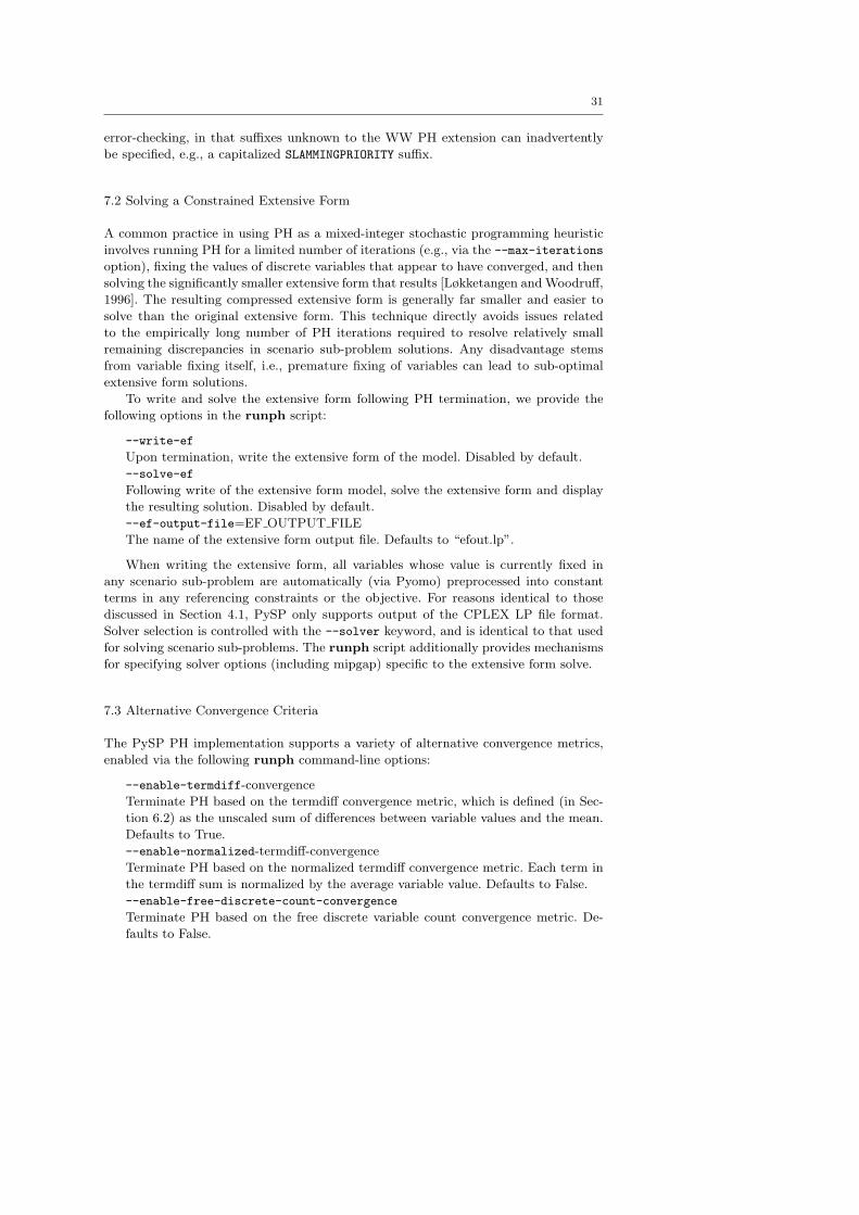
31

error-checking, in that suffixes unknown to the WW PH extension can inadvertently

be specified, e.g., a capitalized SLAMMINGPRIORITY suffix.

7.2 Solving a Constrained Extensive Form

A common practice in using PH as a mixed-integer stochastic programming heuristic

involves running PH for a limited number of iterations (e.g., via the --max-iterations

option), fixing the values of discrete variables that appear to have converged, and then

solving the significantly smaller extensive form that results [Løkketangen and Woodruff,

1996]. The resulting compressed extensive form is generally far smaller and easier to

solve than the original extensive form. This technique directly avoids issues related

to the empirically long number of PH iterations required to resolve relatively small

remaining discrepancies in scenario sub-problem solutions. Any disadvantage stems

from variable fixing itself, i.e., premature fixing of variables can lead to sub-optimal

extensive form solutions.

To write and solve the extensive form following PH termination, we provide the

following options in the runph script:

--write-ef

Upon termination, write the extensive form of the model. Disabled by default.

--solve-ef

Following write of the extensive form model, solve the extensive form and display

the resulting solution. Disabled by default.

--ef-output-file=EF OUTPUT FILE

The name of the extensive form output file. Defaults to “efout.lp”.

When writing the extensive form, all variables whose value is currently fixed in

any scenario sub-problem are automatically (via Pyomo) preprocessed into constant

terms in any referencing constraints or the objective. For reasons identical to those

discussed in Section 4.1, PySP only supports output of the CPLEX LP file format.

Solver selection is controlled with the --solver keyword, and is identical to that used

for solving scenario sub-problems. The runph script additionally provides mechanisms

for specifying solver options (including mipgap) specific to the extensive form solve.

7.3 Alternative Convergence Criteria

The PySP PH implementation supports a variety of alternative convergence metrics,

enabled via the following runph command-line options:

--enable-termdiff-convergence

Terminate PH based on the termdiff convergence metric, which is defined (in Sec-

tion 6.2) as the unscaled sum of differences between variable values and the mean.

Defaults to True.

--enable-normalized-termdiff-convergence

Terminate PH based on the normalized termdiff convergence metric. Each term in

the termdiff sum is normalized by the average variable value. Defaults to False.

--enable-free-discrete-count-convergence

Terminate PH based on the free discrete variable count convergence metric. De-

faults to False.

32

--free-discrete-count-threshold=FREE DISCRETE COUNT THRESHOLD

The convergence threshold associated with the free discrete variable count conver-

gence metric. PH will terminate once the number of free discrete variables drops

below this threshold.

The termination criterion associated with the free discrete variable count is par-

ticularly useful when deployed in in conjunction with the capability to solve restricted

extensive forms described in Section 7.2.

7.4 User-Defined Extensions

The Watson-Woodruff PH extensions described in Section 7.1 are built up a simple,

general callback framework in PySP for developing user-defined extensions to the core

PH algorithm. While most modelers and typical PySP users would not make use of

this feature, programmers and algorithm developers can easily leverage the capability.

The interface for user-defined PH extensions is defined in a PySP read-only file called

phextension.py. The file contents are supplied as follows, to identify the points at

which runph temporarily transfers control to the user-defined extension:

class IPHExtension ( I n t e r f a c e ) :

def p o s t p h i n i t i a l i z a t i o n ( s e l f , ph ) :

””” Cal led a f t e r PH i n i t i a l i z a t i o n . ”””

pass

def p o s t i t e r a t i o n 0 s o l v e s ( s e l f , ph ) :

””” Cal led a f t e r the i t e r a t i o n 0 s o l v e s . ”””

pass

def p o s t i t e r a t i o n 0 ( s e l f , ph ) :

””” Cal led a f t e r the i t e r a t i o n 0 so lve s , averages \computation , and weight update . ”””

pass

def p o s t i t e r a t i o n k s o l v e s ( s e l f , ph ) :

””” Cal led a f t e r the i t e r a t i o n k s o l v e s . ”””

pass

def p o s t i t e r a t i o n k ( s e l f , ph ) :

””” Cal led a f t e r the i t e r a t i o n k so lve s , averages \computation , and weight update . ”””

pass

def pos t ph execut i on ( s e l f , ph ) :

””” Cal led a f t e r PH has terminated . ”””

pass

33

To create a user-defined extension, one simply needs to define a Python class that

implements the PH extension interface shown above, e.g., via the following code frag-

ment:

from pyu t i l i b . component . core import ∗from coopr . pysp import phextens ion

class examplephextension ( S ing l e tonP lug in ) :

implements ( phextens ion . IPHExtension )

def po s t i n s t a n c e c r e a t i o n ( s e l f , ph ) :

print ‘ ‘ Done c r e a t i n g PH sc ena r i o sub−problem in s t an c e s ! ’ ’

# over−r i d e f o r each de f ined c a l l b a c k in phex tens ion . py

. . .

The full example PH extension is supplied with PySP, in the form of the Python

file testphextension.py. All Coopr user plugins are derived from a SingletonPlugin

base class (indicating that there cannot be multiple instances of each type of user-

defined extension), which can for present purposes be viewed simply as a necessary step

to integrate the user-defined into the Coopr framework in which PySP is embedded.

We defer to Hart and Siirola [2010] for an in-depth discussion of the Coopr plugin

framework leveraged by PySP.

Each transfer point (i.e., callback) in the user-defined extension is supplied the PH

object, which includes the current state of the scenario tree, reference instance, all

scenario instances, PH weights, etc. User code can then be developed to modify the

state of PH (e.g., current solver options) or variable attributes (e.g., fixing as in the

case of the Watson-Woodruff extension).

To use a customized extension with runph, the user invokes the command-line op-

tion --user-defined-extension=EXTENSIONFILE. Here, EXTENSIONFILE is the Python

module name, which is assumed to be either in the current directory or in some direc-

tory specified via the PYTHONPATH environment variable. Finally, we observe that both a

user-defined extension and the Watson-Woodruff PH extension can co-exist. However,

the Watson-Woodruff extension will be invoked prior to any user-defined extension.

8 Solving PH Scenario Sub-Problems in Parallel

One immediate benefit to embedding PySP and Pyomo in a high-level language such

as Python is the ability to leverage both native and third-party functionality for dis-

tributed computation. Specifically, Python’s pickl module provides facilities for object

serialization, which involves encoding complex Python objects – including Pyomo in-

stances – in a form (e.g., a byte stream) suitable for transmission and/or storage. The

third-party, open-source Pyro (Python Remote Objects) package [PYRO, 2009] pro-

vides capabilities for distributed computing, building on Python’s pickl serialization

functionality.

34

PySP currently supports distributed solves, accessible from both the runef and

runph scripts. At present, only a simple client-server paradigm is supported in the

publically available distribution. The general distributed solver capabilities provided

in the Coopr library are discussed in Hart et al. [2010], including the mechanisms and

scripts by which name servers (used to locate distributed objects) and solver servers

(daemons capable of solving MIPs, for example) are initialized and interact. Here, we

simply describe the use of a distributed set of solver servers in the context of PySP.

Both the runef and runph scripts are implemented such that all requests for the

solution of (mixed-integer) linear problems are mediated by a “solver manager”. The

default solver manager in both scripts is a serial solver manager, which executes all

solves locally. Alternatively, a user can invoke a remote solver manager by specifying

the command-line option --solver-manager=pyro. The remote (pyro) solver manager

identifies available remote solver daemons, serializes the relevant Pyomo model instance

for communication, and initiates a solve request with the daemon. After the daemon

has solved the instance, the solution is returned to the remote solver manager, which

then transfers the solution to the invoking script.

The accessibility of remote solvers within the PySP PH implementation immedi-

ately confers the benefit of trivial parallelization of scenario sub-problem solves. In

the case of commercial solvers, all available licenses can be leveraged. In the open-

source case, cluster solutions can be deployed in a straightforward manner. Parallelism

in PySP most strongly benefits stochastic mixed-integer program solves, in which the

difficulty of scenario sub-problems masks the overhead associated with object serializa-

tion and client-server communication. At the same time, parallel efficiency necessarily

decreases as the number of scenarios increases, due to high variability in mixed-integer

solve times and the presence of barrier synchronization points in PH (after Step 4 in the

pseudocode introduced in Section 6.1). However, parallel efficiency is of increasingly

diminishing concern relative to the need to support high-throughput computing.

For solving the extensive form, remote solves serve a different purpose: to facilitate

access to a central computing resources, with associated solver licenses. For example,

our primary workstation for developing PySP is a 16-core workstation with a large

amount of RAM (96GB). All commercial solver licenses are localized to this worksta-

tion, which in turn exposes parallelism enabled by now-common multi-threaded solver

implementations.

Given the growing availability of cluster-based computing resources and the in-

creasing accessibility of solver licenses (as is particularly the case for academics, with

access to free licenses for most commercial solvers), the use of distributed computation

by PySP users is expected to continue to grow.

9 Conclusions

Despite the potential of stochastic programming to solve real-world decision problems

involving uncertainty, the use of this tool in industry is far from widespread. Historical

impediments include the lack of stochastic programming support in algebraic model-

ing tools and the inability to experiment with and customize stochastic programming

solvers, which are immature relative to their deterministic counterparts.

We have described PySP, an open-source software tool designed to address both

impediments simultaneously. PySP users express stochastic programs using Pyomo,

an open-source algebraic modeling language co-developed by the authors. In addition

35

to exhibiting the benefits of open-source software, Pyomo is based on the Python

high-level programming language, allowing generic access and manipulation of model

elements. PySP is also embedded within Coopr, which provides a wide range of solver

interfaces (both commercial and open-source), problem writers, solution readers, and

distributed solvers.

PySP leverages the features of Python, Pyomo, and Coopr to develop model-

independent algorithms for generating and solving the extensive form directly, and

solving the extensive form via scenario-based decomposition (PH). The resulting PH

implementation is highly configurable, broadly extensible, and trivially parallelizable.

PySP serves as a novel case study in the design of generic, configurable, and extensi-

ble stochastic programming solvers, and illustrates the benefits of integrating the core

algebraic modeling language within a high-level programming language.

PySP has been used to develop and solve a number of difficult stochastic mixed-

integer, multi-stage programs, and is under active use and development by the authors

and their collaborators. PySP ships with a number of academic examples that have been

used during the development effort, including examples from Birge and Louveaux’s

test, a network flow problem [Watson and Woodruff, 2010], and a production planning

problem [Jorjani et al., 1999]. Real-world applications that have either been completed

in PySP or are under active investigation include biofuel network design [Huang, 2010],

forest harvesting [Badilla, 2010], wind farm network design, sensor placement, and

electrical grid generation expansion.

In-progress and future PySP development efforts include new solvers (e.g., the L-

shaped method), scenario bundling techniques, and support for large-scale parallelism.

In addition, we have recently integrated capabilities for confidence interval estimation

on solution quality.

Both PySP and the Pyomo algebraic modeling language upon which PySP is based

are actively developed and maintained by Sandia National Laboratories. Both are pack-

ages distributed with the Coopr open-source Python project for optimization, which is

now part of the COIN-OR open-source initiative [COIN-OR, 2010].

Acknowledgements

Sandia National Laboratories is a multi-program laboratory operated by Sandia Cor-

poration, a wholly owned subsidiary of Lockheed Martin company, for the U.S. De-

partment of Energy’s National Nuclear Security Administration under contract DE-

AC04-94AL85000. This research was funded from the Office of Scientific Computing

Research within the DOE Office of Science as part of the Complex Interconnected Dis-

tributed Systems program. The authors would like to acknowledge several early users

of PySP and Pyomo, whose (occasionally painful) experience dramatically improved

the quality and design of the software: Yueyue Fan (UC Davis), Yongxi Huang (UC

Davis), Chien-Wei Chen (UC Davis), and Fernando Badilla Veliz (University of Chile).

Appendix: Getting Started

Both PySP and the underlying Pyomo modeling language are distributed with the

Coopr software package. All documentation, information, and source code related to

Coopr is maintained on the following web page: https://software.sandia.gov/trac/

36

coopr. Installation instructions are found by clicking on the Download tab found on the

Coopr main page, or by navigating directly to https://software.sandia.gov/trac/

coopr/wiki/GettingStarted. A variety of installation options are available, including

directly from the project SVN repositories or via release snapshots found on PyPi. Two

Google group e-mail lists are associated with Coopr and all contained sub-projects,

including PySP. The coopr-forum group is the main source for user assistance and

release announcements. The coopr-developers group is the main source for discussions

regarding code issues, including bug fixes and enhancements. Much of the information

found at https://software.sandia.gov/trac/coopr is mirrored on the COIN-OR

web site (https://projects.coin-or.org/Coopr); similarly, a mirror of the Sandia

SVN repository is maintained by COIN-OR.

References

AIMMS. Optimization software for operations research applications.

http://www.aimms.com/operations-research/mathematical-programming/

stochastic-programming, July 2010.

Antonio Alonso-Ayuso, Laureano F. Escudero, and M. Teresa Ortuno. BFC, a branch-

and-fix coordination algorithmic framework for solving some types of stochastic pure

and mixed 0-1 programs. European Journal of Operational Research, 151(3):503–519,

2003.

AMPL. A Modeling Language for Mathematical Programming. http://www.ampl.com,

July 2010.

Fernando Badilla. Problema de Planificacion Forestal Estocastico Resuelto a Traves del

Algoritmo Progressive Hedging. PhD thesis, Facultad de Ciencias Fisicas y Matem-

aticas, Universidad de Chile, Santiago, Chile, 2010.

Dimitri P. Bertsekas. Constrained Optimization and Lagrange Multiplier Methods.

Athena Scientific, 1996.

J.R. Birge and F. Louveaux. Introduction to Stochastic Programming. Springer, 1997.

J.R. Birge, M.A. Dempster, H.I. Gassmann, E.A. Gunn, A.J. King, and S.W. Wallace.

A standard input format for multiperiod stochastic linear program. COAL (Math.

Prog. Soc., Comm. on Algorithms) Newsletter, 17:1–19, 1987.

C.C. Caroe and R. Schultz. Dual decomposition in stochastic integer programming.

Operations Research Letters, 24(1–2):37–45, 1999.

COIN-OR. COmputational INfrastructure for Operations Research. http://www.

coin-or.org, July 2010.

CPLEX. http://www.cplex.com, July 2010.

T.G. Cranic, X. Fu, M. Gendreau, W. Rei, and S.W. Wallace. Progressive hedging-

based meta-heuristics for stochastic network design. Technical Report CIRRELT-

2009-03, University of Montreal CIRRELT, January 2009.

Y. Fan and C. Liu. Solving stochastic transportation network protection problems

using the progressive hedging-based method. Networks and Spatial Economics, 10

(2):193–208, 2010.

FLOPCPP. Flopc++: Formulation of linear optimization problems in c++. https:

//projects.coin-or.org/FlopC++, August 2010.

R. Fourer and L. Lopes. A management system for decompositions in stochastic pro-

gramming. Annals of Operations Research, 142:99–118, 2006.

37

R. Fourer and L. Lopes. Stampl: A filtration-oriented modeling tool for multistage

recourse problems. INFORMS Journal on Computing, 21(2):242–256, 2009.

Robert Fourer, David M. Gay, and Brian W. Kernighan. AMPL: A mathematical

programming language. Management Science, 36:519–554, 1990.

GAMS. The General Algebraic Modeling System. http://www.gams.com, July 2010.

H.I. Gassmann and A.M. Ireland. On the formulation of stochastic linear programs

using algebraic modeling languages. Annals of Operations Research, 64:83–112, 1996.

H.I. Gassmann and E. Schweitzer. A comprehensive input format for stochastic linear

programs. Annals of Operations Research, 104:89–125, 2001.

GUROBI. Gurobi optimization. http://www.gurobi.com, July 2010.

William E. Hart and John D. Siirola. The PyUtilib component architecture. Technical

report, Sandia National Laboratories, 2010.

William E. Hart, Jean-Paul Watson, and David L. Woodruff. Python optimization

modeling objects (pyomo). Submitted to Mathematical Programming Computation,

2010.

T. Helgason and S.W. Wallace. Approximate scenario solutions in the progressive

hedging algorithm: A numerical study. Annals of Operations Research, 31(1–4):425–

444, 1991.

Y. Huang. Sustainable Infrastructure System Modeling under Uncertainties and Dy-

namics. PhD thesis, Department of Civil and Environmental Engineering, University

of California, Davis, 2010.

L.M. Hvattum and A. Løkketangen. Using scenario trees and progressive hedging for

stochastic inventory routing problems. Journal of Heuristics, 15(6):527–557, 2009.

S. Jorjani, C.H. Scott, and D.L. Woodruff. Selection of an optimal subset of sizes.

International Journal of Production Research, 37(16):3697–3710, 1999.

Peter Kall and Janos Mayer. Stochastic Linear Programming: Models, Theory, and

Computation. Springer, 2005a.

Peter Kall and Janos Mayer. Applications of Stochastic Programming, chapter Building

and Solving Stochastic Linear Programming Models with SLP-IOR. MPS-SIAM,

2005b.

S. Karabuk. An open source algebraic modeling and programming software. Technical

report, University of Oklahoma, School of Industrial Engineering, Norman, OK, 2005.

S. Karabuk. Extending algebraic modeling languages to support algorithm develop-

ment for solving stochastic programming models. IMA Journal of Management

Mathematics, 19:325–345, 2008.

S. Karabuk and F.H. Grant. A common medium for programming operations-research

models. IEEE Software, 24(5):39–47, 2007.

LINDO. LINDO systems, August 2010.

O. Listes and R. Dekker. A scenario aggregation based approach for determining a

robust airline fleet composition. Transportation Science, 39:367–382, 2005.

A. Løkketangen and D. L. Woodruff. Progressive hedging and tabu search applied to

mixed integer (0,1) multistage stochastic programming. Journal of Heuristics, 2:

111–128, 1996.

Maximal Software. http://www.maximal-usa.com/maximal/news/stochastic.html,

July 2010.

G. Mitra, P. Valente, and C.A. Poojari. Applications of Stochastic Programming, chap-

ter The SPInE Stochastic Programming System. MPS-SIAM, 2005.

G.R. Parija, S. Ahmed, and A.J. King. On bridging the gap between stochastic integer

programming and mip solver technologies. INFORMS Journal on Computing, 16:

38

73–83, 2004.

PYRO. Python remote objects. http://pyro.sourceforge.net, July 2009.

Python. Python programming language – official website. http://python.org, July

2010a.

Dive Into Python. http://diveintopython.org/power of introspection/index.

html, July 2010b.

R.T. Rockafellar and R.J.-B. Wets. Scenarios and policy aggregation in optimization

under uncertainty. Mathematics of Operations Research, 16(1):119–147, 1991.

R. Schultz and S. Tiedemann. Conditional value-at-risk in stochastic programs with

mixed-integer recourse. Mathematical Programming, 105(2–3):365–386, February

2005.

Alexander Shapiro, Darinka Dentcheva, and Andrzej Ruszczynski. Lectures on Stochas-

tic Programming: Modeling and Theory. Society for Industrial and Applied Mathe-

matics, 2009.

R.M. Van Slyke and R.J. Wets. L-shaped linear programs with applications to optimal

control and stochastic programming. SIAM Journal on Applied Mathematics, 17:

638–663, 1969.

SMI. SMI. https://projects.coin-org.org/Smi, August 2010.

J. Thenie, Ch. van Delft, and J.-Ph. Vial. Automatic formulation of stochastic programs

via an algebraic modeling language. Computational Management Science, 4(1):17–

40, January 2007.

C. Valente, G. Mitra, M. Sadki, and R. Fourer. Extending algebraic modelling lan-

guages for stochastic programming. INFORMS Journal On Computing, 21(1):107–

122, 2009.

Stein W. Wallace and William T. Ziemba, editors. Applications of Stochastic Program-

ming. Society for Industrial and Applied Mathematics, 2005.

J.P. Watson and D.L. Woodruff. Progressive hedging innovations for a class of stochas-

tic mixed-integer resource allocation problems. Computational Management Science

(to appear), 2010.

D.L. Woodruff and E. Zemel. Hashing vectors for tabu search. Annals of Operations

Research, 41(2):123–137, 1993.

Xpress-Mosel. http://www.dashopt.com/home/products/products sp.html, July

2010.

XpressMP. FICO express optimization suite. http://www.fico.com/en/products/

DMTools/pages/FICO-Xpress-Optimization-Suite.aspx, July 2010.

pysp: modeling and solving stochastic programs in … manuscript no. (will be inserted by the...

Documents