CAST---Module 2: Building Module ©Pittsburgh Supercomputing Center Page 1

Module 2A

Deriving a Mathematical Model: An Experimental and Virtual Approach via

Spreadsheets

Using a “Just add data” Excel spreadsheet, we will build a mathematical model

based on data collected using easily obtained resources such as Styrofoam cups.

We will then explore the mathematical model and its physical significance by

introducing parameters to the model, examining measurement error via simulation,

and interpreting the goodness-of-fit for the line of best-fit. Assessment

questions for students that probe their understanding of the model will also be

covered. This module will demonstrate the power of Excel in visualizing data. No

prior Excel experience is needed.

We will also introduce participants to some important aspects of mathematical

modeling as graphing data in Excel, linear regression and interpreting the

goodness-of-fit, and the concepts of interpolation and extrapolation. We will

derive another linear model for some distance versus time data for the Hawaiian

Islands.

Materials needed

Computers with Excel and Internet access

Excel files: stacking_cups.xls

regression.xls

interpol_extrapol.xls

http://seattlecentral.edu/qelp/sets/073/s073.xls

Styrofoam cups

30 cm metric rules (marked to the nearest millimeter)

Part I: Measuring the Stack Height of Nested Styrofoam Cups

Is there a relationship between the height of nested Styrofoam cups and the

number of cups nested? If yes, elaborate on it.

CAST---Module 2: Building Module ©Pittsburgh Supercomputing Center Page 2

Measure the stack heights of various stacks of nested Styrofoam cups. Record

their heights to the nearest 0.1 cm. Record the cup volume: ______

What is the dependent variable?

Deriving the Model

The collected data can be entered into the accompanying

“Just Add Data” Excel spreadsheet on the generate a model tab

(http://academic.pgcc.edu/~ssinex/excelets/stacking_cu

ps.xls). This will determine the line of best-fit by a linear

regression performed on the data. This regression is

your mathematical model! A measure of the goodness of

fit for the regression is given by r2. A perfect fit of the

model to the data would yield an r2 = 1. Record your equation in terms of the

variables studied (not x and y) and the value of r2 here.

What does the equation you found for the data mean?

Number

of nested

cups

Stack

height

(cm)

CAST---Module 2: Building Module ©Pittsburgh Supercomputing Center Page 3

What does the slope represent in terms of the variables investigated?

What are the units of the slope?

What does the y-intercept represent in terms of the variables investigated?

What are the units of the y-intercept?

Now let’s use the equation to make some predictions. What is the height of 150

nested Styrofoam cups? Explain the mathematics used to determine the height.

How many cups are required to obtain a height of 55 cm? Explain the mathematics

used to determine this number.

You have a mathematical model of the nested cups of the form:

H = slope x n + intercept

where H is the height of the nested stack and n is the number of cups.

CAST---Module 2: Building Module ©Pittsburgh Supercomputing Center Page 4

Simulating with the Mathematical Model

Now go to the simulate with model tab and notice we have the capability to change

a couple of parameters related to the cup – rim height and base height.

How does changing the height of the rim influence the regression line on the

graph?

How does changing the height of the base influence the regression line on the

graph?

Now rewrite your mathematical model to incorporate base height and rim height.

For the Styrofoam cups you used, what are the numerical values of the parameters

based on the regression results:

height of the rim: _____ height of the base: _____

For the cups used, are these parameters above realistic? Can you tell anything

about the uniformity of cup manufacturing? Explain.

Suppose we have to pack stacks of cups into cardboard boxes for shipping. How

many cups could be in a stack to fit into a 61 cm long box? …into a 100 cm long

box?

To calculate the results above, what did you do algebraically?

CAST---Module 2: Building Module ©Pittsburgh Supercomputing Center Page 5

The Value of the Inverse Function

Go to the inverse function tab and plot the data with the x and y variables

reversed on the graph.

Write the equation of the inverse function in terms of the variables studied.

How are the original function and the inverse function related? (You may want to

turn on the y = x line on the graph to help.)

How does the goodness of fit behave for the inverse function? Explain.

CAST---Module 2: Building Module ©Pittsburgh Supercomputing Center Page 6

Examining Error in the Model

Go to the simulate errors tab and you will find five different errors to investigate

for this mathematical model. Error can come from measurement (the calibrated

device and its use) and/or the manufacturing process of the cup.

Add each error, one at a time, to see how it influences the data and regression line.

Set each back to no error before going to the next error.

Errors* Slope of line y-intercept Scatter of data

Random

measurement error

Systematic

measurement error

Rim

uniformity

Base uniformity

single stack

Base uniformity

multiple stacks

*read the comment boxes on the Excelet for further explanation of the various errors

Do any of the errors above have a direction or bias (always positive or negative)?

If so, explain.

When you made your measurements earlier, did the ruler and your use of it induce

any error? Did you correct it? Could you correct it?

CAST---Module 2: Building Module ©Pittsburgh Supercomputing Center Page 7

Assessment

Here is a model measured in centimeters: H = 2.0n + 8.0 What is the equation for

the model in inches? (1 inch = 2.54 cm)

Using the model that you derived from the data, how would the model be modified

to handle the stacking of the cups without nesting them (see illustration)? Explain

and sketch a graph.

On a separate sheet of paper, complete the questions on the assessment tab and

attached it to this handout.

CAST---Module 2: Building Module ©Pittsburgh Supercomputing Center Page 8

Notes to the Instructors

This activity allows for the construction of a linear model using the stacking of

nested Styrofoam cups of any size. Measurements should be made to the nearest

0.1 cm (1 mm) using centimeter rulers. Your model with be of the form:

H = slope x n + y-intercept

Where H is the stack height in cm and n is the number of nested cups. The r2

value for the model should be relatively high (close to 1.0) due to the consistent

manufacturing of the Styrofoam cups, if students make the measurements

carefully. If students are not careful, they usually add random scatter to the data

and lower the r2 value.

The slope of the graph represents the height of the rim of the cup, while the y-

intercept is the height of the base of the cup. This leads to some student

confusion as to why the graph has an intercept, since common sense says that zero

cups have zero height. But this model is not a direct proportion like the stacking

of cookies or blocks. The simulation tab on the Excelet will clear this up.

A common error with many 30 cm rulers is that the zero centimeter mark may not

be at the end of the ruler. This induces a constant systematic error. Students

may or may not notice this. Meter sticks do have the zero mark at the end.

Errors Slope of line y-intercept Scatter of data

Random measurement

error (small changes) (small changes)

r2 decreases –adds

scatter

Systematic

measurement error No effect

Positive – intercept

increases

Negative - intercept

decreases

No effect

Rim

uniformity (small changes) (small changes)

r2 decreases –adds

scatter

Base uniformity single

stack No effect

Taller - intercept

increases

Shorter - intercept

decreases

No effect

Base uniformity multiple

stacks (small changes) (small changes)

r2 decreases –adds

scatter

CAST---Module 2: Building Module ©Pittsburgh Supercomputing Center Page 9

For further materials on mathematical modeling and developing interactive Excel

spreadsheets, see the Developer’s Guide to Excelets at

http://academic.pgcc.edu/~ssinex/excelets.

Part II: Elements of Mathematical Modeling

Spreadsheets, such as MS Excel or Open Office Calc, are a very useful

computational tool and easy for students to learn. They allow experimentally-

collected data or other data sets to be graphically analyzed and mathematically

modeled. Here we provide some of the basics to get you started modeling data.

Linear Regression in a Nutshell

The goal of linear regression is to minimize the sum of the squared deviations (the

deviations are the green vertical lines on the graph of the screenshot below).

Open the Excel file: http://academic.pgcc.edu/~ssinex/regression.xls. By

adjusting the slope and intercept, you can minimize the sum of the squared

deviations to see how close you can get by eyeballing it. Then you can add the

computer-based calculation.

The goodness-of-fit can be judged by the minimizing the sum of the squared

deviations. The smaller the sum of the squared deviations the better the line fits

the data points. The value of r2 is a numerical way of expressing the minimized

sum of the squared deviations (search RSQ in MS Excel help for more info). An r2

CAST---Module 2: Building Module ©Pittsburgh Supercomputing Center Page 10

value of one is a perfect fit of the data. An r2 value can be interpreted as the

fraction of the y-value variation that is explained by the variation in the x-variable.

The plot of the residues or the deviations (see deviations tab) is another way of

judging goodness-of-fit, especially for discovering non-linear relationships that

appear to be linear.

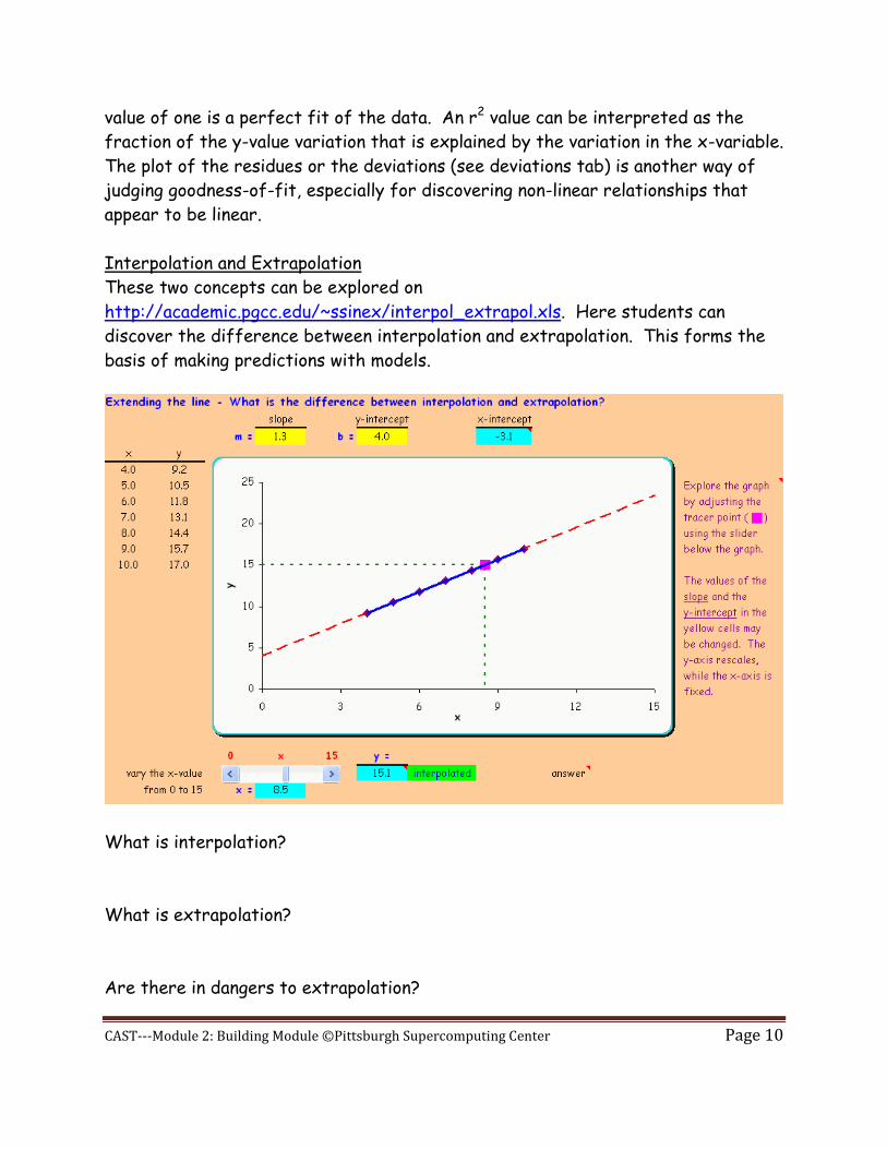
Interpolation and Extrapolation

These two concepts can be explored on

http://academic.pgcc.edu/~ssinex/interpol_extrapol.xls. Here students can

discover the difference between interpolation and extrapolation. This forms the

basis of making predictions with models.

What is interpolation?

What is extrapolation?

Are there in dangers to extrapolation?

CAST---Module 2: Building Module ©Pittsburgh Supercomputing Center Page 11

The dangers of extrapolation can be explored on the aluminum can data tab as well.

CAST---Module 2: Building Module ©Pittsburgh Supercomputing Center Page 12

Graphing and Modeling Data

Let’s examine the age of the various

Hawaiian Islands as a function of distance

from the Big Island and develop a

mathematical model for the rate of

movement for the Pacific plate.

Download the Excel file - http://seattlecentral.edu/qelp/sets/073/s073.xls

How does the age of the volcanic island vary with distance from the Big Island of

Hawaii? To address this question let’s plot a graph of the age of the various

Hawaiian Islands as a function of distance from the Big Island. Here we want to

graph the data as a scatter plot in Excel. The scatter plot is the only graph in

Excel where the x-axis is plotted as a variable (and not a category). Follow the

steps outlined on the screenshot below.

CAST---Module 2: Building Module ©Pittsburgh Supercomputing Center Page 13

Once you have the graph on the worksheet, you will need to label axes, title, and

remove the gridlines.

Developing a mathematical model requires us to add a trendline using a linear fit of

the data on the graph.

With the graph selected, click on the

Trendline button dropdown arrow to get the

list and select the More Trendlines Option…

at the bottom.

CAST---Module 2: Building Module ©Pittsburgh Supercomputing Center Page 14

Then the Format Trendline menu will appear as seen below. The default setting is

linear is shown here to the left.

Then you need to select the Display Equation

on chart and Display R-squared value on chart.

You need to do this every time you perform a

regression!

Now press the Close button and view your

graph.

Write the equation found in terms of the

variables studies (not x and y). Record the

value of r2.

How good a fit is the line to the data?

What does the slope of the linear regression tell us?

Has the rate of the Pacific plate over time been fairly constant? Explain.

How old would an island be at distance of 5500 km? Explain how you accomplished

this.

For the background information on this data set:

http://www.seattlecentral.edu/qelp/sets/073/073.html

(The map shown earlier is from this website.)

CAST---Module 2: Building Module ©Pittsburgh Supercomputing Center Page 15

More Data and Spreadsheet Resources

Exploring Linear Data from NCTM -

http://illuminations.nctm.org/LessonDetail.aspx?id=L298

Quantitative Environmental Learning Project (QELP) – has linear and a variety of

other non-linear data sets with explanations in a number of different formats

including Excel - http://seattlecentral.edu/qelp/Data.html

Two other interactive Excel spreadsheets dealing with linear models –

Stacking cookies

http://academic.pgcc.edu/~ssinex/cookies_stack.xls

http://academic.pgcc.edu/~ssinex/cast/cookies_stack.pdf

Burning candles

http://academic.pgcc.edu/~ssinex/excelets/burning_candles.xls

http://academic.pgcc.edu/~ssinex/excelets/burning_candles_act.pdf

References

If you want more on the scatter of data, outliers and how they influence linear

models including a discussion of residuals for goodness-of-fit, see -

S.A. Sinex (2005) Exploring the Goodness of Fit in Linear Models, Journal of

Online Mathematics and its Application 5.

If you want more on random and systematic error in data, see -

S.A. Sinex (2005) Investigating Types of Errors, Spreadsheets in Education 2 (1)

115-124.

S.A. Sinex, B.A. Gage, and P.J. Beck (2007) Exploring Measurement Error with Cookies: A Real and Virtual Approach via Interactive Excel, The AMATYC Review

29 (1) 46-53. (Excelet)

For a further discussion of the nested Styrofoam cup model, see-

S.A. Sinex (2008) Scientific and Algebraic Thinking: Visualizing with Interactive Excel and Nested Styrofoam Cups, On-Line Proceedings of the 34th Annual

CAST---Module 2: Building Module ©Pittsburgh Supercomputing Center Page 16

Conference of the American Mathematical Association of Two-Year Colleges in

Washington, DC.