1

Bridging the aviation CO2 emissions gap: why emissions trading is needed D. S. Lee*, L. L. Lim and B. Owen Dalton Research Institute, Department of Environmental and Geographical Sciences, Manchester Metropolitan University, John Dalton Building, Chester Street, Manchester M1 5GD, UK

* Author for correspondence. E-mail: d.s.lee@mmu.ac.uk

Abstract: Total aviation emissions in 2006 were 630 Mtonnes CO2, 62% of which were international and 38% domestic. By 2050, total aviation emissions are projected to be between approximately 1,000 to 3,100 Mtonnes CO2, depending upon growth and level of mitigation assumed (technology, operations, biofuels, market-based mechanisms–MBMs). The Kyoto Protocol includes only domestic emissions of aviation CO2, whereas international emissions currently fall to the International Civil Aviation Organization (ICAO) to “limit or reduce” under Article 2.2 for Annex I Parties. Emission ‘goals’ for international aviation have been set by various parties: ICAO has a 2% yr-1 fuel efficiency improvement goal; a medium term aspirational goal of no net increase in international aviation emissions from 2020; a goal of carbon-neutral growth by 2020 compared with 2005 levels was proposed to the ICAO 37th General Assembly by Canada, Mexico and the US; and a 10% reduction on the 2005 level was proposed by the European Union. Baseline international CO2 emissions from aviation were 391 Mtonnes in 2006, and these increased under the extremes of the ranges of growth (low/central/high) and mitigation scenarios to between approximately 600 and 2,000 Mtonnes CO2 by 2050 (1.5 to 5 fold increase). Under a central growth scenario, international emissions were projected to increase to 1,638 Mtonnes CO2 by 2050 assuming ‘business-as-usual’ (BAU) emissions reductions from technology and operational improvements, or 1,306 Mtonnes CO2 by 2050 under a ‘Maximum feasible reductions’ (MFR) scenario of mitigation from technology and operational improvements. The additional usage of “likely1” biofuel availability reduced BAU 2050 emissions by 5% (to 1,556 Mtonnes CO2); “speculative” biofuel availability reduced the MFR technology and operations-reduced 2050 emissions by 15% (to 1,110 Mtonnes CO2). If one considers the additional reductions to BAU/MFR technological and operational improvements from extending existing regional MBMs beyond their current 2020 limit to 2050 (i.e. in the absence of biofuels), BAU emissions would be reduced by 36% (to 1,051 Mtonnes CO2) and MFR emissions by 33% (to 877 Mtonnes CO2). Combining both biofuels and the extension of existing regional MBMs reduces BAU 2050 emissions by 38% (to 1,008 Mtonnes CO2), and MFR emissions by 41% (to 774 Mtonnes CO2). As a single measure, current regional MBMs extended to 2050 deliver the largest emission reductions. In terms of achievement of 2050 goals, the MFR technology/operations scenario cannot achieve the 2% yr-1 fuel efficiency goal by either 2020 or 2050 for any of the growth scenarios. Addition of a ‘speculative’ level of biofuels just manages to exceed the 2% yr-1 goal by 2050 by between -10 and -62 Mtonnes CO2. Addition of the existing regional MBMs to technology/operational improvements extended to 2050 (i.e. no biofuels) exceeds the 2% goal by between -54 and -388 Mtonnes CO2. Combining all three types of measure exceeds the 2% goal by between -86 and -516 Mtonnes CO2. None of the measures analysed, or their combinations, achieve the goal of 2020 carbon neutrality by 2050 for any growth scenario, and an ‘emissions gap’ of between approximately 70 to 1,430 Mtonnes CO2 remains by 2050; similarly, a gap remains between all measures and stabilization of emissions at 2005 levels, by 2050, with an emissions gap of between approximately 230 to 1,640 Mtonnes CO2 in 2050 and 270 to 1,680 Mtonnes CO2 for 10% below 2005 levels by 2050. Given that the current regional MBMs extended to 2050 achieved the single largest reduction, as a measure, an operational and effective global scheme would evidently achieve even greater reductions.

1 The biofuel availability and life cycle analysis of the UK Committee on Climate Change has been adopted in this work who define three scenarios of availability; ‘likely’, ‘optimistic’, ‘speculative’ – see body of text for full details.

2

1 Introduction

Aviation is a strongly-growing transport sector of economic and social importance. Global air traffic in Revenue Passenger Kilometres (RPK) has increased by a factor of 2.5 between 1990 and 2010, and a factor of 1.6 between 2000 and 20102. Periods of world-influencing events such as oil crises, war, terrorism, and economic downturns have consistently been followed by periods of growth (Lee et al., 2009). Even with the recent global economic crisis, RPK increased by 28% between 2005 and 2010. Whilst regional patterns of traffic are more complex, there is still a strong demand at a global level for aviation. Aviation currently uses kerosene for powering aircraft engines, and is likely to do so into the foreseeable future. At present, virtually all kerosene is derived from fossil fuels, and thus adds to other anthropogenic CO2 emissions resulting in climate change. Aviation also has other emissions and effects that result in an overall warming of climate (IPCC, 1999) that may account for around 5% of total radiative forcing (RF) – the commonly-used climate metric to measure impacts – but the CO2 RF impacts are the most well understood and quantified (Lee et al., 2009). Emissions of CO2 are also different to other RF aircraft impacts in that, in common with all anthropogenic CO2 emissions, the residual warming effects may last many thousands of years (IPCC, 2007a – Chapter 7). Aviation CO2 emissions are currently ~2 to 2.5% of present-day CO2 emissions (Lee et al., 2009). The most recent comprehensive assessment of civil aviation CO2 emissions is for a baseline year of 2006, from extensive work contributed by states3 under the aegis of the International Civil Aviation Organization’s Committee on Aviation and Environmental Protection (ICAO-CAEP) (ICAO, 2010). Emissions of CO2 from civil aviation in 2006 were 630 Mtonnes, 62% of which (391 Mtonnes yr-1) were international and 38% (239 Mtonnes yr-1) domestic. Total aviation emissions (including military emissions) can be estimated from International Energy Agency data on kerosene fuel sales (IEA, 2009) and were 743 Mtonnes yr-1 in 2006. A number of scenarios of future aviation CO2 emissions have been made, and Lee et al. (2011) provide a convenient review (see Figure 1). Virtually all scenarios in the literature result in increases in emissions by 2050 over those in 2006. Currently and historically, increased aviation demand has outstripped CO2 emissions reductions through technological and operational improvements (IPCC, 1999). The reasons for this are that aircraft have high fuel-efficiency, and development is mostly constrained by incremental technological improvements, with rather limited scope to improve global emissions from improved operations. Moreover, the global fleet is replaced only rather slowly, and new types of aircraft have long development timescales to entry into service, and have in-service lifetimes of the order 25 years.

2 See data from http://www.airlines.org/Pages/Annual-Results-World-Airlines.aspx accessed 26-02-2013 3 Including the present authors on behalf of the UK

3

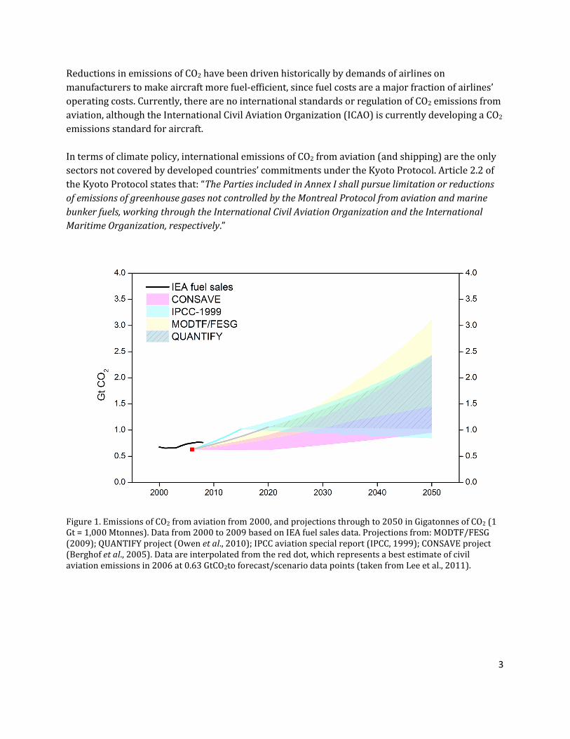
Reductions in emissions of CO2 have been driven historically by demands of airlines on manufacturers to make aircraft more fuel-efficient, since fuel costs are a major fraction of airlines’ operating costs. Currently, there are no international standards or regulation of CO2 emissions from aviation, although the International Civil Aviation Organization (ICAO) is currently developing a CO2 emissions standard for aircraft. In terms of climate policy, international emissions of CO2 from aviation (and shipping) are the only sectors not covered by developed countries’ commitments under the Kyoto Protocol. Article 2.2 of the Kyoto Protocol states that: “The Parties included in Annex I shall pursue limitation or reductions of emissions of greenhouse gases not controlled by the Montreal Protocol from aviation and marine bunker fuels, working through the International Civil Aviation Organization and the International Maritime Organization, respectively.”

Figure 1. Emissions of CO2 from aviation from 2000, and projections through to 2050 in Gigatonnes of CO2 (1 Gt = 1,000 Mtonnes). Data from 2000 to 2009 based on IEA fuel sales data. Projections from: MODTF/FESG (2009); QUANTIFY project (Owen et al., 2010); IPCC aviation special report (IPCC, 1999); CONSAVE project (Berghof et al., 2005). Data are interpolated from the red dot, which represents a best estimate of civil aviation emissions in 2006 at 0.63 GtCO2to forecast/scenario data points (taken from Lee et al., 2011).

4

A recent report of the United Nations Environment Programme (UNEP), “Bridging the Emissions Gap” (UNEP, 2011), considered the mitigation potential of a number of sectors, including aviation (Lee et al., 2011), in the context of progress towards a 2 degree target4 at 2020. Here, we extend the concept of that work on the mitigation potential of aviation emissions out to 2050. Rather than considering aviation in the context of 2 degrees, as the UNEP work did, the focus of the work presented here is to examine whether there is an emissions ‘gap’ between various scenarios of aviation emissions reductions by 2050, ranging from a ‘business-as-usual’ (BAU) type of situation through to one of ‘maximum feasible reductions’ (MFR) and the various declared goals for the sector, and the size of the resultant gap(s). Here, the work is expanded substantially to consider 2050 projections for total and international aviation, and the potential CO2 emissions savings from technology and operational improvements, and utilization of biofuels. In addition, the potential CO2 emissions savings from existing market-based mechanisms (MBMs) are considered.

4 The so called ‘2 degree target’ refers to a target not to exceed a global mean surface temperature increase by more than 2 degrees C over that of the preindustrial period, usually taken to be 1750.

5

2 An evaluation of emissions-reductions potential: data, methods and assumptions

Future scenarios of fleet growth and technological and operational improvements Here, we consider a range of projections of aviation emissions for 2050 taken from work for ICAO’s CAEP and estimate the mitigation potential for 2050 from technology, operational improvements, biofuels, and market based measures. ICAO’s CAEP considered three scenarios of traffic growth to 2050 (low, central, high) and translated these traffic projections into emissions by various assumptions of fleet growth, aircraft replacements, their size and technology, and differential patterns of growth of traffic in and between regions (MODTF/FESG, 2009; Anon, 2010). Six fuel-burn ‘mitigation’ scenarios were considered, S1 through to S55. Here, only scenarios S2 through to S5 are considered, since S1 only envisaged growth of the fleet based on influx of best of 2010 technology forward to 2050. Scenarios S2 to S5 are summarized as follows: S2 – low aircraft technology and moderate operational improvements; S3 – moderate aircraft technology and operational improvements; S4 – advanced technology and operational improvements; S5 – optimistic technology and operational improvements. No assumptions were made over particular policies that would drive the MODTF/FESG (2009) projections but the scenarios did specifically exclude biofuels. These scenarios illustrate plausible emission pathways. Here, we consider S2 as a business-as-usual scenario of technological and operational improvements, and S5 as maximum feasible reductions6.

S2 was chosen as a 'business-as-usual' case, since it was based on assumptions similar to those documented by IPCC (1999). This was based on historical rates of fleet fuel efficiency improvements that were 1.3% yr-1 and projected to be 1.0% yr-1 from 2010 onwards. S2 assumes improvements of 0.95%-1 for all new aircraft (note, that this is aircraft fuel efficiency, not total global fleet) entering the fleet after 2006 and 0.57% yr-1 from 2015 to 2036. Operational improvements were 0.5, 1.4 and 2.3 percent in 2016, 2026 and 2036, respectively. By contrast, S3 had continuing fuel efficiency improvements of 0.96% yr-1 for all aircraft entering the fleet after 2006 to 2036 and the same operational improvements as S2. Thus, S3 envisages no 'flattening off' of

5 Note that a change in scenario nomenclature occurred between MODTF/FESG (2009) and that summarized in Anon. (2010) - the original ‘S1’ scenario was a parametric variant of the original frozen technology ‘S2’ (now described as S1) but with no operational improvements leading to an overall deterioration in ATM efficiency. This S1 was subsequently removed to simplify the presentation of mitigation options and scenario numbers were subsequently then changed S#+1. Here, we adhere to the most recent S1 to S5 nomenclature of Anon. (2010). 6 MODTF/FESG (2009) note that S5 (previously S6) is a “…sensitivity study that goes beyond the improvements based on industry-based recommendations”.

6

technological improvements, which has been widely considered in the literature (see IPCC, 1999; IPCC, 2007b – Chapter 5) to be likely. Mitigation from biofuels Since MODTF/FESG (2009) did not consider biofuels, their mitigation potential is considered here. Low-carbon alternatives to aviation kerosene may include biofuels, although associated indirect emissions must be considered. Lifecycle reductions of up 80% have been claimed (IATA, 2009); the emissions associated with land-use change vary significantly but may reduce carbon-savings or even lead to an increase in carbon emissions (Stratton et al., 2010).

The UK Committee on Climate Change (UKCCC) made a comprehensive evaluation of the potential for biofuels based upon the work of the International Energy Agency (IEA, 2008) and work commissioned by the Committee on Climate Change (E4Tech, 2009) for its report on aviation (UKCCC, 2009). Given this detailed biofuel assessment, which was a global one, the UKCCC projections of biofuel uptake and CO2 life-cycle savings are used here.

The UKCCC estimated that the contribution of biofuels might be 10% by 2050 under what was described as a “likely” scenario, 20% for an “optimistic” scenario, and 30% for a “speculative” scenario (UKCCC, 2009). In all cases, the UKCCC assumed a 50% life-cycle CO2 saving, such that the percentages became 5% (likely), 10% (optimistic), and 15% (speculative). A 2% market penetration of biofuels by 2020 was deemed feasible by other work (Novelli, 2011); this is similar to UKCCC’s assumptions for 2030, ranging from less than <2% (likely), through 3% (optimistic), to 5% (speculative) market penetration.

In producing incremental projections that consider the additional mitigation potential through the uptake of biofuels to the technology/operational scenarios (MODTF/FESG, 2009; Anon., 2010), the “likely” biofuel scenario is applied to S2, the “optimistic” biofuel scenario is applied to S3 and S4, and the “speculative” biofuel scenario applied to S5. As in the UKCCC (2009) work, a 50% life-cycle CO2 saving is assumed in all cases.

In this work the primary objective is to understand emissions mitigation potential over a 'base case' in which no biofuels are present, in other words, the marginal improvements gained over a 'do nothing' case. Hence, following the approach of e.g. UKCCC (2009), ATAG7, and Sustainable Aviation (Sustainable Aviation, 2012), the change in carbon footprint from aviation is represented in the analysis, hence the life-cycle factor is accounted for when presenting emissions reductions.

Market-Based Measures (MBMs)

Two basic types of MBMs attach a price to emissions: charges, such as taxes/levies; and the use of carbon markets such as offsets or cap-and-trade instruments including tradable emissions rights/allowances/permits. In the aviation sector, the only mandatory operational schemes at the

7 http://www.atag.org/facts-and-figures.html

7

international level are currently cap-and-trade systems: domestic flights are included in the New Zealand Emissions Trading Scheme (ETS); and both domestic and international flights are included in the EU ETS, which began in 2012 (see Preston et al., 2012 for an overview). However, the EU-ETS for aviation has recently been suspended for one year8 for non-EU international arriving and departing flights under the “stop the clock” initiative so that a global scheme can be discussed within ICAO that might replace the EU’s scheme (European Commission, 2012a,b).

The EU-ETS covers all international arriving and departing flights from non-EU countries, and departing flights intra-EU international flights, and all domestic flights in EU states. The cap at the outset of the scheme in 2012 is 97% of the mean calculated 2004–2006 aviation emissions (of the order 221 Mtonnes CO2), falling to 95% in 2013. The emissions under the EU scheme were calculated for this work with a global aviation inventory/scenario model, ‘FAST’ for 2006 emissions (see Preston et al., 2012), and non-EU international departing/arriving, intra-EU international, and EU domestic emissions were calculated separately.

Goals for international aviation At its 2010 37th General Assembly, the International Civil Aviation Organization (ICAO) agreed to work to achieve a goal of a global annual average 2% fuel efficiency improvement per year until 2020, and a continued aspirational goal of 2% improvement per year until 2050 on the basis of volume of fuel used per revenue tonne kilometre (ICAO, 2010). This is referred to here as the ‘2% yr-1 fuel efficiency goal’. In addition to the 2% yr-1 fuel efficiency goal, ICAO also resolved at the 37th General Assembly that it would work together with its Member States and relevant organizations “to strive to achieve a collective medium term global aspirational goal of keeping the global net carbon emissions from international aviation from 2020 at the same level…” This is referred to here as the ‘2020 carbon-neutral goal’. Here, the 2020 carbon-neutral goal has been defined as a band, given the uncertainty of emissions, such that it spans the S2 BAU to the 2% yr-1 fuel efficiency line in 2020.

Over and above these goals, a Working Paper to the 37th General Assembly of ICAO by Canada, Mexico and the US proposed “4.2 Regarding a more ambitious, global goal to address international civil aviation CO2 emissions: ―The Assembly resolves that ICAO and its Contracting States shall strive to achieve a collective global goal of carbon-neutral growth by 2020 based on a 2005 baseline.” (Working Paper A37-WP/186, 2010). This is referred to here as the ‘2005 stabilization goal’. In addition to this, a paper to the 37th Assembly presented by Belgium (on behalf of the European Union and Member States, Members of the European Civil Aviation Conference, and EUROCONTROL) states in para 2.6 that “Accordingly the EU has advocated that the global reduction target for greenhouse gas emissions from international aviation should be a 10% reduction by 2020 compared to 2005 levels” (Working paper A37-WP/108, 2010). This is referred to here as the ’2005-10% stabilization goal’.

8 At the time of writing, this is still formally a proposal, as it requires a co-decision procedure between EU Member States and the European Parliament before being formally adopted and agreed.

8

3 Results – calculated emissions reductions

Mitigation from technology and operations alone Using the data from the MODTF/FESG scenarios, aviation emissions of CO2 according to different technological and operational mitigation scenarios for total and international aviation are given in Table 1. Table 1. Emission of aviation CO2 in 2050 (Mtonnes yr-1), according to MODTF/FESG (2009); low, central, and high traffic growth scenarios and technological/operational mitigation scenarios S2 (business as usual) through to S5 (maximum feasible reductions) Total aviation

(Mtonnes CO2 yr-1)

Growth scenario S2 S3 S4 S5 Low 1,841 1,717 1,604 1,468 Central 2,504 2,335 2,182 1,996 High 3,105 2,895 2,705 2,475 International

aviation (Mtonnes CO2 yr-1)

Growth scenario S2 S3 S4 S5 Low 1,204 1,123 1,049 960 Central 1,638 1,527 1,427 1,306 High 2,031 1,894 1,769 1,619 Mitigation from technology, operations, and biofuels Using the assumptions outlined above in section 2 on application of biofuel availability, and effective life-cycle CO2 reductions of 50%, additional savings on CO2 emissions are calculated and the resultant emissions given in Table 2.

Table 2. Emissions of aviation CO2 in 2050 (Mtonnes yr-1), accounting for varying levels of biofuel availability, and a 50% life-cycle reduction (see text for details). Total aviation

(Mtonnes CO2 yr-1)

Growth scenario S2 S3 S4 S5 Low 1,749 1,545 1,444 1,247 Central 2,379 2,102 1,964 1,697 High 2,949 2,606 2,435 2,104 International

aviation (Mtonnes CO2 yr-1)

Growth scenario S2 S3 S4 S5 Low 1,144 1,011 944 816 Central 1,556 1,374 1,284 1,110 High 1,929 1,704 1,592 1,376

9

Mitigation from technology, operations, and existing regional MBMs The potential mitigation from existing regional MBMs required additional calculations to qualify this. Using the global FAST inventory model, Preston et al. (2013) calculated aviation CO2 emissions under the scope of the EU-ETS were 204 Mtonnes of CO2 for 2006 (comparing favorably with the Commission’s own calculation of 221 Mtonnes CO2, 2004 – 2006 average). These emissions broke down into 135 Mtonnes CO2 from non-EU international arriving and departing flights, 51 Mtonnes CO2 from intra-EU international flights, and 17 Mtonnes CO2 from EU domestic flights. The total of 204 Mtonnes CO2 was 35% of global emissions in 2006, or 48% of international emissions (i.e. excluding the 17 Mtonnes CO2 EU domestic emissions). This calculation was necessary in order to subtract the domestic contribution of the EU-ETS for projections of international emissions, and the contribution of MBMs. However, that the EU scheme covered 35% of emissions in future years could not be assumed, so this was explicitly calculated. Using regionally disaggregated traffic statistics trends from MODTF/FESG (2009) and assumed rates of improvements in technology for the S2BAU case, the fractional coverage of the EU-ETS was calculated for the 2036 projection of traffic, the limits of MODTF/FESG’s (2009) projections (extrapolation to 2050 was used after 2036). In the event, the overall global fractional coverage was found to be the same in 2036, but with differing regional-flow contributions. The inter/intra-regional percentages of emissions in 2036 are given in Table 3.

Table 3. Fractions of CO2 emissions calculated for route-groups covered under the scope of the EU-ETS and their relative growth over time to 2036

Route Int’l/Domestic 2006 2036 North Atlantic Int’l 23% 17% South Atlantic Int’l 3% 3% Mid Atlantic Int’l 5% 6% Europe–Asia Int’l 19% 22% Europe–Africa Int’l 8% 9% Europe–Middle East Int’l 6% 10% Sub-total EU–non-EU Int’l 65% 67% Intra Europe Intra-Int’l 28% 26% Europe Domestic 8% 7% total EU-ETS 100% 100% Percentage EU-ETS of global total 35.5% 35.0%

Table 3 indicates that whilst emissions on some routes grow at a faster rate than others, as expected, the overall emissions under the scheme coverage, when summed, still represent around 35% of global emissions in 2036. We assume that this fraction then stays constant from 2036 until 2050, in the absence of data to calculate regional traffic emissions projections. In addition, it is assumed that the EU-ETS cap stays constant from 2020 to 2050. In addition, it is recognized that the ETS has a small effect on demand, and emissions are reduced as a result. For this, we utilize the analysis of CE-Delft et al. (2007) who projected an in-sector saving of 11 Mtonnes CO2 in 2020 of the EU-ETS. We assume that this remains a constant fraction of the EU-ETS coverage of emissions and

10

correct for this in the global and international totals. The emissions for the combination of technological and operational improvement scenarios S2–S5 and the extension of existing regional MBMs from 2020 to 2050 are given in Table 4. Table 4. Emission of aviation CO2 in 2050 (Mtonnes yr-1), accounting for varying levels of technology and operational improvements (S2 to S5), and continuation of the regional MBMs from 2020 to 2050 at the same level of cap. Total aviation

(Mtonnes CO2 yr-1)

Growth scenario S2 S3 S4 S5 Low 1,426 1,344 1,269 1, 179 Central 1,864 1,752 1,651 1,528 High 2,260 2,122 1,997 1,845 International

aviation (Mtonnes CO2 yr-1)

Growth scenario S2 S3 S4 S5 Low 824 781 743 696 Central 1,051 993 941 877 High 1,257 1,185 1,120 1,041 Mitigation from technology, operations, and existing regional MBMs Lastly, the three types of mitigation measures are combined, and the emissions in 2050 for all three growth-scenarios for total and international aviation are given in Table 5. Table 5. Emission of aviation CO2 in 2050 (Mtonnes yr-1), accounting for varying levels of technology and operational improvements (S2 to S5), biofuel uptake, and continuation of the regional MBMs from 2020 to 2050 at the same level of cap. Total aviation

(Mtonnes CO2 yr-1)

Growth scenario S2 S3 S4 S5 Low 1,365 1,230 1,163 1,034 Central 1,781 1,598 1,507 1,330 High 2,158 1,931 1,818 1,599 International

aviation (Mtonnes CO2 yr-1)

Growth scenario S2 S3 S4 S5 Low 792 722 687 620 Central 1,008 913 866 774 High 1,204 1,086 1,027 914 The emission trends over time for these emissions calculations for total and international aviation emissions from 2006 to 2050 are shown in Figures 2 and 3.

11

Figure 2. Total aviation emission projections, 2006 – 2050 (Mtonnes CO2 yr-1), central growth scenario, showing ranges of emissions by mitigation type and combination. Upper of all bands is ‘S2’ (business-as-usual); lower of all bands is ‘S5’ (maximum feasible reductions) – see text for details of how mitigation options are combined.

Figure 3. International aviation emission projections, 2006 – 2050 (Mtonnes CO2 yr-1), central growth scenario, showing ranges by mitigation type and combination. Upper of all bands is ‘S2’ (business-as-usual); lower of all bands is ‘S5’ (maximum feasible reductions) – see text for details of how mitigation options are combined.

12

4 Discussion

Mitigation by type of measure Using the data shown in Figure 3, the central growth scenario for international emissions to 2050 can be shown by each individual measure, or combination of measures, separately for more clarity, as in Figure 4.

Figure 4. International aviation emission projections, 2006 – 2050 (Mtonnes CO2 yr-1) showing ranges by individual mitigation type and combination. Panel A shows emissions by ‘technology & operations’ mitigation options only; panel B, technology & operations combined with biofuels; panel C technology & operations combined with current MBMs projected to 2050; panel D all mitigation options together (technology & operations, biofuels, MBMs). The upper of all bands is ‘S2’ (business-as-usual); lower of all bands is ‘S5’ (maximum feasible reductions) – see text for details of how mitigation options are combined. Figure 4 shows that the technology and operational improvements (central growth scenario) span the range of 1,638 to 1,306 Mtonnes CO2 in 2050 (S2 to S5); if biofuels are added, then the S2 BAU emissions are reduced by 5% (S2 bio) to 1,556 Mtonnes CO2, and the S5 MFR emissions combined with speculative levels of biofuels are reduced by 15% from 1,306 to 1,110 Mtonnes CO2, see Figure 4, panel B. If the existing regional MBMs are added to the S2 BAU,

13

S5 MFR emissions, then the reductions in CO2 emissions are 36% and 33%, respectively (from 1,638 to 1,051 Mtonnes of CO2, and from 1,306 to 877 Mtonnes CO2 in 2050), see Figure 4, panel C. Combining all measures, reduces the emissions of S2 BAU, S5 MFR by 38% and 41% respectively (from 1,638 to 1,008 Mtonnes of CO2, and from 1,306 to 744 Mtonnes CO2 in 2050), see Figure 4, panel D. In terms of ‘effectiveness’, the emissions reductions from the extension of the existing regional MBMs are clearly the largest; even if an S2 BAU technology scenario is assumed, the MBMs reduce these emissions by 36%. Extending S2 to S5 alone reduces emissions by approximately 20%. The projections assume a number of things: that the technological/operational improvements can be driven as far as the S5 MFR emissions; that the biofuels can substitute up to 30% of the kerosene by 2050 (at 50% C life-cycle effectiveness); and that the existing regional MBMs operate at the same level of cap and that the C savings can be made elsewhere and sufficient permits can be bought at prices that do not reduce demand beyond what has already been calculated by CE-Delft et al. (2007) for 2020 and extrapolated further as a proportion of emissions to 2050. Considering technology and operations, MODTF/FESG (2009) notes of scenario S5 “This sensitivity study goes beyond the improvements based on industry-based recommendations.” It includes optimistic fuel burn improvements of 1.5% yr-1 for all aircraft entering the fleet after 2006 to 2036, and “additional fleet-wide optimistic operational improvements of 3.0, 6.0 and 6.0 percent by 2016, 2026 and 2036, respectively”. In terms of the biofuels, the assumptions from UKCCC (2009) are regarded as “speculative”, representing high availability from the underlying studies of E4Tech (2009) and IEA (2008) that informed the UKCCC (2009) analysis. In the case of extending the existing regional MBMs, it has been assumed that this operates out to 2050, and with the same cap as planned for up to 2020. The assumption of emissions trading is that as the market innovates and adapts, the cap is lowered, so the assumption of a static cap to 2050 is conservative. However, on the other hand, it also assumes that C savings can be made to that magnitude out to 2050 and that emission permits can be bought at reasonable costs that do not affect demand more than is already assumed. In terms of ‘effectiveness’, the emissions reductions from the extension of the existing regional MBMs are clearly the largest; even if an S2 BAU technology scenario is assumed, the MBMs reduce these emissions by 36% with no additional requirements on improvements from technology and operations over BAU. Extending S2 to S5 alone reduces emissions by approximately 20%. In order to achieve this change (from S2 to S5), this would assume policy in place to drive such “optimistic” technological/operational improvements, along with large investment in research and development to achieve them. This is only one comparison in a potential suite of options: what would be informative – beyond the scope of this study – is a study of cost-effectiveness of the different options in a marginal abatement cost-curve study. This may be difficult given the long time-frame of 2050 and the lack of data, but should be considered as, on the face of it, the existing regional MBMs extended to 2050 seems to offer an attractive lower-cost option, given sufficient carbon savings elsewhere in other sectors. If one imagined a global MBM scheme (with the caveat of sufficient carbon savings elsewhere), then the savings could be much larger.

14

The context of different growth scenarios The time-series charts shown in this paper (e.g. Figures 2 – 4) have focused on the underlying central traffic projection, or ‘growth scenario’ of MODTF/FESG (2009). In order to understand how the various technological, operational, biofuel and MBM measures reduce emissions relative to assumptions over different rates of traffic growth, ‘end point’ emissions for 2050 are shown in Figure 5 for total and international aviation.

Figure 5. Total aviation CO2 emissions by mitigation scenario and by growth scenario at 2050 (upper panel); international aviation CO2 emissions by mitigation scenario and by growth scenario at 2050 (lower panel).

15

Figure 5 combines the data given in Tables 1, 2, 4 and 5 in a readily understood manner. Clearly, the level of demand for aviation in terms of the growth projections makes a substantial difference to the absolute magnitude of the emissions and the potential abatement opportunities, showing the large uncertainties in the absolute outcomes. For example, one can see that both for total and international aviation, the BAU S2 technology and operations scenario for the low demand scenario is at a similar level to the lower end of the central growth, more stringent technology and higher biofuels range. Similarly, a high growth scenario would imply achieving at least the S5 technology/operational scenario to be approximately on a par with the central S2 BAU scenario. Evidently, the growth aspects represent a significant uncertainty (in common with most aviation emissions scenarios that have been developed). ‘Emissions gap’ analysis Having calculated the range of potential outcomes of the different mitigation options, concentrating once again (but not exclusively) on the central growth scenario, for illustrative purposes, the ‘emissions gap’ between mitigation option projections and the 2% yr-1 fuel efficiency, 2020 carbon-neutral, 2005 stabilization of emissions (by 2050), and the 2005-10% stabilization of emissions (by 2050) goals can be calculated. Table 6 provides a complete assessment of the gap or degree of compliance (negative numbers) between the full range of scenarios in terms of mitigation options, and combinations, and traffic growth scenarios.

16

Table 6. Emissions gaps (positive numbers) and emission compliances (negative numbers) between various goals and mitigation options, by growth scenarios at 2050.

These emission gaps and compliances with goals are shown for the central growth scenario in Figure 6 for the 2% yr-1 fuel efficiency goal, Figure 7 for the 2020 carbon-neutral goal, Figure 8 for the 2005 stabilization of emissions goal, and Figure 9 for the 2005-10% stabilization of emissions goal (see Appendix I for a figure of 2006 – 2050 emissions, central growth scenario shown against all goals).

17

Figure 6. International aviation emission projections, 2006 – 2050 (Mtonnes CO2 yr-1), for central growth scenario. Emission ‘gaps’ between projections and ‘2% yr-1 fuel efficiency goal’ are shown as ranges by mitigation type, and combination. Upper of all bands is ‘S2’ (business-as-usual); lower of all bands is ‘S5’ (maximum feasible reductions) – see text for details of how mitigation options are combined.

Figure 7. International aviation emission projections, 2006 – 2050 (Mtonnes CO2 yr-1), for central growth scenario. Emission ‘gaps’ between projections and 2020 ‘Carbon-neutral goal’ are shown as ranges by mitigation type, and combination. Upper of all bands is ‘S2’ (business-as-usual); lower of all bands is ‘S5’ (maximum feasible reductions) – see text for details of how mitigation options are combined.

18

Figure 8. International aviation emission projections, 2006 – 2050 (Mtonnes CO2 yr-1), for central growth scenario. Emission ‘gaps’ between projections and ‘2005 stabilization of emissions by 2050 goal’ are shown as ranges by mitigation type, and combination. Upper of all bands is ‘S2’ (business-as-usual); lower of all bands is ‘S5’ (maximum feasible reductions) – see text for details of how mitigation options are combined.

Figure 9. International aviation emission projections, 2006 – 2050 (Mtonnes CO2 yr-1), for central growth scenario. Emission ‘gaps’ between projections and ‘2005-10% stabilization of emissions by 2050 goal’ are shown as ranges by mitigation type, and combination. Upper of all bands is ‘S2’ (business-as-usual); lower of all bands is ‘S5’ (maximum feasible reductions) – see text for details of how mitigation options are combined.

19

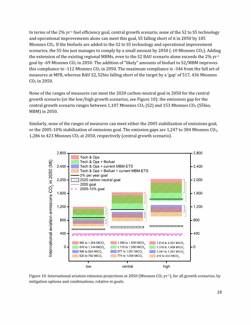
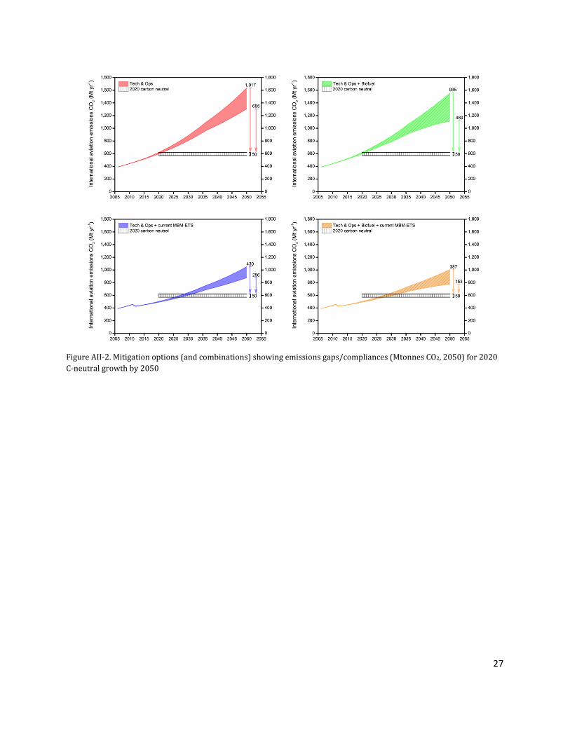
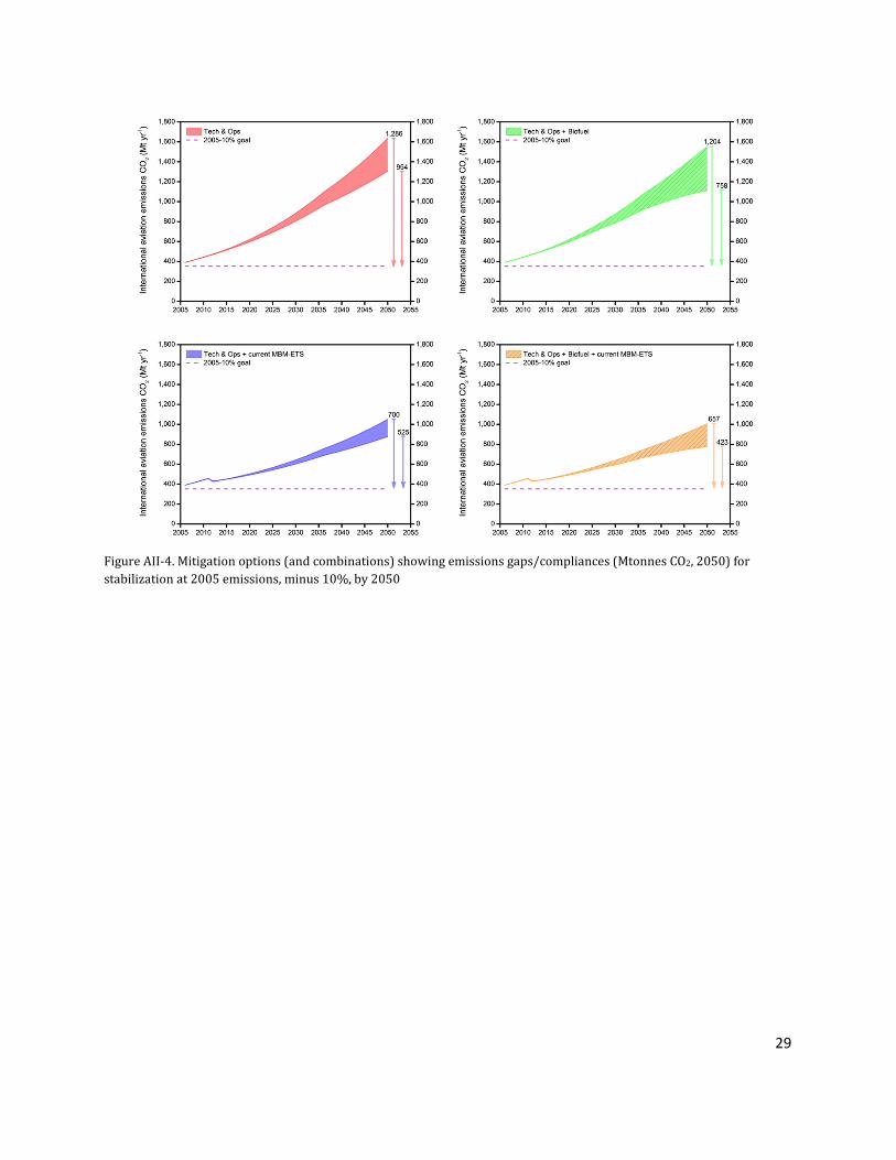
In terms of the 2% yr-1 fuel efficiency goal, central growth scenario, none of the S2 to S5 technology and operational improvements alone can meet this goal, S5 falling short of it in 2050 by 185 Mtonnes CO2. If the biofuels are added to the S2 to S5 technology and operational improvement scenarios, the S5-bio just manages to comply by a small amount by 2050 (-10 Mtonnes CO2). Adding the extension of the existing regional MBMs, even to the S2 BAU scenario alone exceeds the 2% yr-1 goal by -69 Mtonnes CO2 in 2050. The addition of “likely” amounts of biofuel to S2/MBM improves this compliance to -112 Mtonnes CO2 in 2050. The maximum compliance is -346 from the full set of measures at MFR, whereas BAU S2, S2bio falling short of the target by a ‘gap’ of 517, 436 Mtonnes CO2 in 2050. None of the ranges of measures can meet the 2020 carbon-neutral goal in 2050 for the central growth scenario (or the low/high growth scenarios, see Figure 10): the emissions gap for the central growth scenario ranges between 1,107 Mtonnes CO2 (S2) and 153 Mtonnes CO2 (S5bio, MBM) in 2050. Similarly, none of the ranges of measures can meet either the 2005 stabilization of emissions goal, or the 2005-10% stabilization of emissions goal. The emission gaps are 1,247 to 384 Mtonnes CO2, 1,286 to 423 Mtonnes CO2 at 2050, respectively (central growth scenario).

Figure 10. International aviation emission projections at 2050 (Mtonnes CO2 yr-1), for all growth scenarios, by mitigation options and combinations, relative to goals.

20

‘Emissions gap’ or trajectory? How the effectiveness of scenarios might be calculated. Ultimately, what most emissions-gap analyses are addressing is how CO2 projected emissions fit in, or otherwise, with a so-called ‘2 degrees trajectory’. As outlined in the introduction, a common goal under the UNFCCC discussions, as reiterated in the COP18 Doha Agreed Outcome Pursuant to the Bali Action Plan (Draft Decision -/CP.18) is to limit the increase in global mean surface temperatures by 2°C by 2100 over pre-industrial values. The background and basis of a ‘2 degree target’, in the context of aviation, has been set out by Lee et al. (2013). If a temperature-based target is the objective, then the emissions rate, at any given point in time (e.g. 2050), is largely irrelevant. This is because CO2 emissions accumulate in the atmosphere and are removed only slowly at varying rates of uptake, according to the sink (IPCC, 2007a – Chapter 7). Thus, the emissions either in total, or of a sector at, say 2050, are only indicative of an overall emissions trajectory. In order to calculate a temperature response, CO2 emissions need to be considered in a historical perspective, or the present-day CO2 concentration considered. The CO2 concentrations then need to be calculated for some future emissions scenario using a C-cycle model that considers sources, sinks and preferably feedbacks. From the resultant CO2 concentrations, the radiative forcing can then be calculated relatively easily via a parameterized formula. The temperature response can then be calculated, most often for scenario analysis, from a simplified climate response model, with some degree of uncertainty over climate sensitivity. From this simplified description of model-processes required to calculate a temperature response, it can be understood that in terms of aviation’s contribution to climate change through its CO2 emissions, it is not the arbitrary ‘end point’ (here, we have focused on 2050) emissions that matter so much as “how one got there”, or, to a first order, cumulative emissions (Allen et al., 2009). A next step from this work to calculate a more meaningful comparative measure of efficacy of various emissions scenarios is to calculate the marginal CO2 concentrations, radiative forcing, and temperature response with, for example, a simplified climate response model on the different emissions pathways, or ‘trajectories’ to 2050.

21

5 Conclusions & recommendations

From baseline emissions of 630 Mtonnes of CO2 in 2006, total aviation emissions are projected to increase to between 1,034 and 3,105 Mtonnes of CO2 by 2050. This emission range encompasses at the extremes, high growth, BAU technology and operational improvements, compared with low growth, MFR technology and operational improvements, “speculative” levels of biofuels and extension of existing regional MBMs at the same cap level to 2050. For international aviation, the similar span of emissions by 2050 is 620 to 2,031 Mtonnes CO2, on a 2006 baseline of 391 Mtonnes CO2.

The mitigation possibilities for 2050 can be compared in a number of ways and combinations in order to understand absolute and relative reductions that may be available. Using the central growth scenario and taking S2 BAU technology and operational improvements as a 'benchmark' (1,638 Mtonnes CO2, 2050) one can conclude the following. The reduction in emissions from introducing a "likely" amount of biofuels to S2 BAU technology and operations is 82 Mtonnes CO2 (5% reduction). The reduction in emissions from introducing extended regional MBMs out to 2050 to S2 BAU technology and operations (i.e. no biofuels) is 587 Mtonnes CO2 (36% reduction). The combined effect of a "likely" amount of biofuels and extending the regional MBMs over the S2 BAU technology and operations scenario is 630 Mtonnes CO2 (39% reduction9). Considering a comparison of S2 BAU technology and operations against more ambitious reductions yields the following. The reduction in emissions from MFR technology and operations (S5) over S2 BAU technology and operations is 332 Mtonnes CO2 (20% reduction). The reduction in emissions from MFR technology and operations (S5) combined with a "speculative" level of biofuels over S2 BAU technology and operations is 528 Mtonnes CO2 (32% reduction). The reduction in emissions from MFR technology and operations over S2 BAU technology introducing extended regional MBMs to 2050 (i.e. no biofuels) is 761 Mtonnes CO2 (47%). The reduction in emissions from MFR technology and operations (S5) combined with a "speculative" level of biofuels, and extension of the regional MBMs over S2 BAU technology and operations is 864 Mtonnes CO2 (53% reduction). The emissions reductions available from the range of BAU to MFR technology and operational improvements did not meet the 2% yr-1 improvement in fuel efficiency for international aviation at any point in time to 2050. When MFR technology and operational improvement reductions were combined with “speculative” levels of biofuels, the 2% goal for international aviation was just exceeded by -10 Mtonnes CO2 in 2050. Any combination of measures that included extension of existing regional MBMs exceeded the 2% goal at any point in time out to 2050.

9 Note that the reductions are not simply additive, because the biofuels are assumed to be a proportion of total fuel, whereas the MBM is against a fixed cap, then proportioned for biofuels, when combined.

22

None of the measures, or their combinations, for any growth scenario managed to meet the 2020 carbon-neutral goal, the 2005 stabilization of emissions goal, or the 2005-10% stabilization of emissions goal at 2050. The maximum reductions over BAU technology and operational improvements were clearly achieved by the extension of the existing MBMs out to 2050. A global scheme constructed on similar lines is likely to achieve more savings, assuming that sufficient C savings can be made outside the aviation sector, and be bought at a price that does not suppress demand more than has already been assumed in the calculations (8.4%). In order to further quantify environmental and the most cost-effective benefits, it is recommended that the CO2 radiative forcing and temperature responses be studied (as these will give a better comparative measure of environmental effectiveness than end-point emissions), and relative costs of the different measures be further studied. REFERENCES

Allen M. R., Frame D. J., Huntingford C., Jones C. D., Lowe J. A., Meinshausen M. and Meinshausen N. (2009) Warming caused by cumulative carbon emissions towards the trillionth tonne. Nature 458 1163–1166.

Anon. (2010) Climate Change Outlook, ICAO Secretariat, Environmental Report 2010. Montreal, Canada: International Civil Aviation Organization. Available at: http://www.icao.int/icao/en/env2010/environmentreport_2010.pdf

Berghof, R., Schmitt, A., Eyers, C., Haag, K., Middel, J., Hepting, M., Grübler, A. & Hancox, R. (2005) CONSAVE 2050 final technical report. Available at: http://www.dlr.de/consave/CONSAVE 2050 Final Report.pdf

CE-Delft, Ecofys, MVA, Lee D. S. (2007) Technical assistance for the impact assessment of inclusion of aviation in the EU ETS. Final Report, CE-Delft, Delft, The Netherlands.

E4Tech (2009) Review of the potential for biofuels in aviation.

European Commission (2012a) European Commission. MEMO/12/854 Stopping the clock of ETS and aviation emissions following last week’s International Civil Aviation Organization (ICAO) Council, (12th November 2012)

European Commission (2012b) Proposal for a Decision of the European Parliament and of the Council derogating temporarily from Directive 2003/87/EC of the European Parliament and of the Council establishing a scheme for greenhouse gas emission allowance trading within the Community.

IATA (2009) Annual Report 2009. Montreal, Canada: International Air Transport Association (IATA). Available at: http://www.iata.org/pressroom/Documents/IATAAnnualReport2009.pdf

ICAO (2008) Guidance on the Use of Emissions Trading for Aviation. International Civil Aviation Organization. First edition, Doc 9885.

ICAO (2010) Environmental Report 2010. Montreal, Canada: International Civil Aviation Organization. Available at: http://www.icao.int/icao/en/env2010/environmentreport_2010.pdf

IEA (2008) Energy Technology Perspectives. Scenarios and Strategies to 2050, International Energy Agency, OECD/IEA, Paris.

IEA (2009) Oil Information 2008, International Energy Agency, Paris.

23

IPCC (1999) Aviation and the Global Atmosphere. Penner, J. E., Lister, D. H., Griggs, D. J., Dokken, D. J. & McFarland, M. eds. Intergovernmental Panel on Climate Change. Cambridge, UK: Cambridge University Press. Available at: http://www.ipcc.ch/ipccreports/sres/aviation/index.htm

IPCC (2007a) Climate Change 2007. The Physical Science Basis. S. Solomon, D. Qin, M. Manning, M. Marquis, K. Averyt, M. M. B. Tignor, H. L. Miller and Z. Chen (eds). Contribution of Working Group I to the Fourth Assessment Report of the Intergovernmental Panel on Climate Change. Cambridge University Press, UK.

IPCC (2007b) Climate Change 2007. Mitigation. B. Metz, O. Davidson, P. Bosch, R. Dave, L. Meyer (eds). Contribution of Working Group III to the Fourth Assessment Report of the Intergovernmental Panel on Climate Change. Cambridge University Press, UK.

Lee D. S., Fahey D., Forster, P., Newton P. J., Wit, R. C. N., Lim L. L., Owen B., and Sausen R. (2009) Aviation and global climate change in the 21st century. Atmospheric Environment 43, 3520–3537.

Lee D. S., Hare, W., Endresen Ø., Eyring V., Faber J., Lockley P., Maurice L., Schaeffer M., Wilson C. (2011) International emissions. In ‘Bridging the Emissions Gap. A UNEP Synthesis Report’. United Nations Environment Programme (UNEP).

Lee D. S., Baughcum S. L., Sausen R., Hileman J. (2013) The role of aviation in a two degree world. Appendix C to Working Paper 31, CAEP 9, Montreal, February 4th to 15th, 2013.

MODTF/FESG (2009) ‘Global aviation CO2 emissions projections to 2050, Agenda Item 2: Review of aviation-emissions related activities within ICAO and internationally’, Group on International Aviation and Climate Change (GIACC) Fourth Meeting. Montreal, 25 - 27 May. Montreal, Canada: International Civil Aviation Organization, Information paper GIACC/4-IP/1.

Novelli, P. (2011) Sustainable Way For Alternative Fuels and Energy in Aviation – Final Report. SWAFEA formal report D.9.2 v1.1 (SW_WP9_D.9.1_ONERA_31.03.2011). Paris, France: ONERA. Available at: http://www.swafea.eu/LinkClick.aspx?fileticket=llISmYPFNxY%3D&tabid=38

Owen B., Lee D. S., Lim L. L. (2010) Flying into the future: aviation emission scenarios to 2050. Environmental Science and Technology 44, 2255–2260.

Preston H., Lee D. S., Hooper, P. D. (2012) The inclusion of the aviation sector within the European Union's Emissions Trading Scheme: what are the prospects for a more sustainable aviation industry? Environmental Development 2, 48 – 56.

Preston H., Lee D. S., Lim L. L., Owen B. (2013) Aviation emissions trading at a crossroads – the question of scope. Manuscript in preparation.

Stratton, R. W., Wong, H. M. & Hileman, J. I. (2010) Life Cycle Greenhouse Gas Emissions from Alternative Jet Fuels. PARTNER Project 28 Report Version 1.2. Boston, MA: Massachusetts Institute of Technology (MIT). Available at: http://web.mit.edu/aeroastro/partner/reports/proj28/partner-proj28-2010-001.pdf

Sustainable Aviation (2012) Sustainable aviation CO2 road-map. Sustainable Aviation group, Available at www.sustainableaviation.co.uk

UKCCC (2009) Meeting the UK aviation target – options for reducing emissions to 2050. London, UK: Committee on Climate Change (CCC). Available at: http://downloads.theccc.org.uk/Aviation%20Report%2009/21667B%20CCC%20Aviation%20AW%20COMP%20v8.pdf

UNEP (2011) ‘Bridging the Emissions Gap. A UNEP Synthesis Report’. United Nations Environment Programme (UNEP).

Working Paper A37-WP/186, (2010) A more ambitions, collective approach to international aviation greenhouse gas emissions. Presented by Canada, Mexico and the United States. A37-WP/186, 37th session of the ICAO Assembly, Montreal, Canada.

24

Working paper A37-WP/108 (2010) Addressing aviation’s environmental impacts through a comprehensive approach. Presented by Belgium on be half of the European Union and its Member States and by the other States Members of the European Civil Aviation Conference, and by Eurocontrol. A37-WP/108, 37th session of the ICAO Assembly, Montreal, Canada.

25

APPENDIX I

Figure A1. International aviation emission projections, 2006 – 2050 (Mtonnes CO2 yr-1) showing ranges by mitigation type and combination. Upper of all bands is ‘S2’ (business-as-usual); lower of all bands is ‘S5’ (maximum feasible reductions) – see text for details of how mitigation options are combined. Emissions are shown in relation to international aviation goals of 2% yr-1 fuel efficiency, Carbon-neutral growth of 2020 emission by 2050; stabilization of 2005 emissions & 10% reduction of stabilization at 2005 emissions.

26

APPENDIX II

Figure AII-1. Mitigation options (and combinations) showing emissions gaps/compliances (Mtonnes CO2, 2050) for 2% yr-1 fuel efficiency goal

27

Figure AII-2. Mitigation options (and combinations) showing emissions gaps/compliances (Mtonnes CO2, 2050) for 2020 C-neutral growth by 2050

28

Figure AII-3. Mitigation options (and combinations) showing emissions gaps/compliances (Mtonnes CO2, 2050) for stabilization at 2005 emissions by 2050

29

Figure AII-4. Mitigation options (and combinations) showing emissions gaps/compliances (Mtonnes CO2, 2050) for stabilization at 2005 emissions, minus 10%, by 2050